Are Exports and Imports Cointegrated DEC 2014...Are Exports and Imports Cointegrated? ......

Babatunde, Journal of International and Global Economic Studies, 7(2), December 2014, 45-67 45

Are Exports and Imports Cointegrated? Evidence from Nigeria

Musibau Adetunji Babatunde

University of Ibadan

Abstract his study examined the long-run relationship between Nigerian exports and imports

between 1960 and 2014. Exports and imports were disaggregated into oil and non-oil

components. The application of the Johansen, Bound testing and the Hansen parameter

instability test cointegration techniques revealed that Nigerian exports and imports at the

aggregate and disaggregated level are cointegrated with the cointegrating coefficient very close

to unity. This indicated that Nigeria's macroeconomic policies have been effective in the long run

and suggested that Nigeria is not in violation of its international budget constraint. The result is

however sensitive to the choice of the dependent variable between exports and imports. Utilizing

the Toda and Yamamoto granger non-causality tests, we also report bi-directional causality

between aggregate exports and imports, but uni-directional causality from oil exports to oil

imports and from non-oil imports to non-oil exports.

Key words: Exports, Imports, Cointegration, Budget Constraint, Nigeria

JEL Classification: C22, F14, F43.

1. Introduction

The important role of exports and imports in the economy cannot be overemphasized. Exports

and imports play an integral role in determining the trade balance of a country. As a result, the

dynamics of the relationship between these two variables hold significant importance for the

economy and have attracted the interest of researchers in testing the nature of relationships

between exports and imports. This is because an unsustainable trade deficit indicates a violation

of international budget constraints over time. If the trade deficits should persist, the domestic

interest rates will be very high and such an economy will metamorphosed into a heavily indebted

country which may affects the welfare of the citizens. Consequently, the presence of a long run

relationship between exports and imports is highly desirable for any economy. The occurrence of

a cointegration relationship between imports and exports suggests that the trade deficits of a

country are short-term and sustainable in the long run and confirm the existence of an effective

macroeconomic policy. Hence, the need to investigate whether trade deficits is only a short-run

phenomenon in Nigeria.

Although the literature has examined the relationship between exports and imports extensively in

the last three decades, it is inconclusive with respect to their cointegration relationship. While

some of the studies have reported long run relationship between exports and imports, other has

found weak or no cointegration. This lack of consensus can be attributed to methodological


problem, selectivity bias, and specification error. By way of illustration, while some of the

studies have adopted exports as the dependent variable, other studies have made use of imports

as the dependent variable, thereby leading to different empirical conclusion. A close observation

of the literature revealed that the results seem to be mixed for cointegration techniques that

require the specification of dependent and independent variables. However, in cointegration tests

that requires variable ordering, the choice of dependent or independent variables seems not to

matter. Since, the choice of the dependent variable adopted can influence the direction of result,

this study examine the cointegration relationship between exports and imports in the context of

the two variables as dependent and independent variables using different cointegration tests. In

addition, we perform a disaggregated analysis by separating imports and exports into oil and

non-oil components. The disaggregation is necessary to determine the extents of co-movement of

the components of exports and imports with respect to achieving sustainable trade balance.

Similarly, some of the studies have reported unidirectional, bi-directional or no causality with

respect to exports and imports. This lack of consistent causal pattern between exports and

imports in the studies may be due to the use of the traditional Granger causality frameworks. The

use of a simple traditional Granger causality test has been identified by several studies (Engle

and Granger, 1987; Toda and Philips, 1993; Toda and Yamamoto, 1995; Dolado and Lutkepohl,

1996; Zapata and Rambaldi, 1997; Tsen, 2006) as not sufficient if variables are integrated of

order one, i.e. I(1) and cointegrated. Many economic time-series are integrated of order one, i.e.

I(1), and when they are cointegrated, the simple F-test statistic does not have a standard

distribution. Hence, the choice of the Toda and Yamamoto’s (1995) Granger non-causality tests

in this study. The Toda and Yamamoto’s test is useful because it allow tests of Granger causality

between exports and imports while accounting for the long-run information often ignored in

systems that require first differencing and pre-whitening prior to inference.

The choice of Nigeria as a case study is justified on several reasons. Nigeria has the largest

population and the biggest economy in Africa. Trade continues to play an important role, with

total trade (imports and exports) accounting for over 53% of GDP. Nigeria has experienced

extensive and rapid trade liberalization, undertaken both in the context of unilateral, regional and

multilateral trade negotiations. With respect to imports, Nigeria is committed to a gradual

elimination of tariffs and to the abolition of non-tariff barriers that have the same effects as

tariffs. As a result, its trade regime has become more liberal with the average applied MFN tariff

falling from 28.6% in 2003 to 11.9% in 2009, due mainly to Nigeria aligning its tariff with that

of the Economic Community of West African States (ECOWAS) common external tariff (CET).

Accordingly, the promotion of exports has been a decisive factor for improving economic growth

and external payments, as part of the economic reform which began in 1986. With respect to

export policies, the Nigerian government has implemented and heavily promoted export

incentives for export-oriented firms' in the last three decades. The most significant measures


include the Export Expansion Grant Fund Scheme (EEG) to increasing exports and diversifying

export products and markets and the Export Development Fund (EDF) to assists in the finance of

certain activities of private exporting companies. In order to support these measures, the

Nigerian government created supporting institutions such as the Nigerian Export Promotion

Council which is saddled with the responsibility of promoting and enhancing the volume and

value of Nigeria’s non-oil export in the international market and diversify the basket of

exportable products from Nigeria and the Nigeria Export-Import Bank to provide export credit

guarantee and export credit insurance facilities to exporters.

Secondly, Nigeria recorded a current account surplus of 7.10 percent of the country's Gross

Domestic Product (GDP) in 2013. Current account to GDP in Nigeria averaged 1.67 percent

from 1980 until 2013, reaching an all-time high of 37.90 percent in 2008 and a record low of -

18.70 Percent in 1986. The strong current account surplus reveals that the Nigerian economy is

still heavily dependent on oil exports revenues, with high savings rate but weak domestic

demand. This implies that Nigeria is providing an abundance of resources to other economies,

and is owed money in return. Thus, by providing these resources abroad, Nigeria with a current

account balance surplus gives other economies the chance to increase their productivity.

However, the problem is whether the current account surplus is sustainable in the long run given

the fluctuations in the crude oil prices in the international oil market. This informed the

examination of the long run relationship between imports and exports for Nigeria.

Thirdly, the choice of Nigeria is also motivated by the fact that there is no known study that has

been conducted to examine the relationship between imports and exports in Nigeria. Tang (2006)

in a study of 27 OIC countries could not proceed with cointegration tests because the variables

were found to be integrated of different order. This is therefore the first major attempt in the

literature to investigate the sustainability of Nigerian trade imbalance by testing for

cointegration. In addition, the knowledge of the direction of causality between imports and

exports is essential for the design and evaluation of current and future macroeconomic policies

aimed at achieving trade balance. The sequence of this study is clear. Section II presents a review

of the previous works on the subject. The methodology of estimation and the specification of the

various equations are highlighted in Section III. This is followed by the estimation results and

interpretation of results in Section IV. Section V concludes.

2. Review of Related Studies

The theoretical and empirical foundation of the examination of cointegration between imports

and exports was laid by Husted (1992). Husted (1992) examined the long run association

between exports and imports of the U.S. Husted used quarterly data of trade for the U. S.

economy. The author concluded a long run relationship between the exports and imports and

found that there was a tendency in U.S. exports and imports to converge in the long run. Export

was used as the dependent variable in the Husted (1992) model. Following the pioneering work


of Husted (1992) several researchers have investigated the long run relationship between exports

and import in both developed and developing countries. However, there is no consensus about

the relation between the long run relationship between exports and imports in the literature

despite the importance of the co-movement of exports and imports as an important factor in the

understanding of the sustainability of trade deficits. While some of the studies have found a long

run relationship between imports and exports, other studies have considered the impact as being

weak, conditional or non-existing.

Among the set of studies that reported the existence of cointegration, Bahmani- Oskooee (1994)

investigated the long-run convergence between Australian imports and exports between 1960

and 1992. The application of the Engle and Granger (1987) cointegration technique revealed that

Australian imports and exports are cointegrated with the cointegrating coefficient very close to

unity which suggested that Australia's macroeconomic policies have been very effective. Using

quarterly data and Johansen and Juselius’s (1990) cointegration technique, Bahmani-Oskooee

and Rhee (1997) found that South Korea’s exports and imports are cointegrated and the

coefficient on exports was positive. This result implies that South Korea does not violate its

international budget constraint.

Also, Arize (2002) using quarterly data 1973-1998 and imports as the dependent variable, found

that 35 of 50 countries in the study sample supported the existence of cointegration between

imports and exports using the Johansen cointegration technique. Nevertheless, using Stock and

Watson’s (1988) cointegration technique as a complementary test to the Johansen, all countries,

except Mexico, revealed the existence of a cointegration relationship between imports and

exports. Arize (2002) therefore, concluded that macroeconomic policies have been effective in

the long run and suggests that these countries are largely not in violation of their international

budget constraints. Using annual data from 1961 to 1999 (full sample period), and the Gregory-

Hansen (1996) cointegration test, Baharumshah, et al. (2003) find support for a cointegration

relationship between imports and exports for Indonesia, the Philippines, and Thailand, but not for

Malaysia.

With a sample of 27 OIC member nations and adopting the Engle and Granger’s cointegration

approach, Tang and Mohammad (2005) found that only four countries exhibited a long-term

relationship between the volume of imports and exports. These countries are Benin, Burkina

Faso, Cameroon and Guyana. They concluded that exchange rate and monetary or fiscal policies

may be effective to improve a country’s trade balance in the long run. Arguing that conventional

results of the unit root test and cointegration may yield unconvincing result, Tang (2006)

reinvestigated the cointegration relationship between imports and exports for the Organization of

the Islamic Conference (OIC) and applied unit root tests with unknown level shift (Lanne,

Lutkepohl and Saikkonen, 2002 and Saikkonen and Lutkepohl, 2002) and the cointegration test

with structural break developed by Gregory and Hansen (1996). Export was used as the


dependent variable in the model. The study revealed that restrictions are not applicable for

testing cointegration between imports and exports for OIC member countries. Interestingly, the

study revealed cointegration between exports and imports for 9 of the 27 selected OIC member

countries (Bangladesh, Cameroon, Chad, Guyana, Indonesia, Mali, Morocco, Niger and Senegal)

compared to only 4 countries as demonstrated by Tang and Mohammad (2005).

More recently, Ali (2013) analyzed the long run association between Pakistan’s exports and

imports. Empirical analysis revealed a long run relationship between the two variables. The error

correction model results showed that exports and imports converge towards the long run

equilibrium. This indicates the effectiveness of macroeconomic policies in stabilizing the

international trade balance in Pakistan. A similar finding was reported by Al-Khulaifi (2013) in

the case of Qatar. Pillay (2014) examined the long run equilibrium relationship between South

Africa’s exports and imports using quarterly data from 1985 to 2012. Adopting the Johansen’s

Maximum Likelihood cointegration technique and using imports as the dependent variable, the

study found a statistically significant cointegrating relationship is found to exist between exports

and imports. This finding is consistent with the results of Herzer and Nowak-Lehman (2006)

which reported cointegration between exports and imports for Chile. Import was used as the

dependent variable in the Herzer and Nowak-Lehman (2006) study.

On the contrary, some other studies reported the non-existence of cointegration between exports

and imports. Fountas and Wu (1999) used quarterly data for the periods 1967-1989 and 1967-

1994 respectively, to examine whether exports and imports are cointegrated in the United States.

The study found no long-run relationship between exports and imports in the case of United

States. Also, Keong et al. (2004) explored the long run relationship between exports and imports

of Malaysia by using cointegration techniques. The study concluded that short run fluctuations

between the imports and exports were not sustainable and the imports and exports would

ultimately converge to towards long run equilibrium. Irandoust and Ericsson (2004) found

cointegrating relationship between exports and imports of some developed economies for

Germany, Sweden, and the United States. But the study did not found any cointegration between

the variables for the UK.

Similarly, Cheong (2005) in a commentary on Malaysian imports and exports argued that

cointegration findings are not conclusive in the case of Malaysian economy. Using annual data

for the period 1959-2000, he applied Johansen cointegration test and no cointegration was found.

Konya and Singh (2008) investigated the presence of equilibrium relationship between exports

and imports in India using annual data for the period from 1949/50 – 2004/05 using exports as

the dependent variable. Indian exports and imports were found to be integrated of order one.

Johansen cointegration method was then performed on data, and failed to reject the no-

cointegration hypothesis. The paper concluded that Indian exports and imports do not exhibit a


cointegration relationship and therefore, India is in violation of its international budget

constraint.

In addition, Dumitriu, et al. (2009) explored the dynamic relations between the Romanian

exports and imports using monthly data from January 2005 to March 2009. They tested the

cointegration and causality between the two variables. The results of Engle-Granger, Johansen

and cointegration tests are ambiguous while the Breitung test infirmed the hypothesis of

cointegration between exports and imports. In these circumstances the study concluded that it

cannot consider Romanian current account deficits as sustainable. Hye and Siddiqui (2010) also

explored the link between exports earnings and imports expenditures for Pakistan using quarterly

data for the period between 1985 and 2008 and utilized imports as the dependent variable. They

applied the variance decomposition method and rolling window bound tests to check the stability

of causal relationship. The study concluded that international budget constraint of Pakistan

unsustainable; hence imports and exports are not cointegrated.

Recently, Hussein (2014) examined the long-run convergence (cointegration) between exports

and imports for nine MENA (Middle East and North Africa) countries. The article explored the

issue by applying the bounds testing approach to cointegration using annual data. Using imports

as the dependent variable, the study reported cointegration between exports and imports for Iran,

Israel, Jordan, and Tunisia indicate that these countries are not in violation of their international

budget constraint. However, it failed to find long run relationship Algeria, Egypt, Morocco,

Sudan, and Syria. The finding from these studies is an indication that the choice of the dependent

variable between exports and imports partly influences the existence of cointegration result that

is reported.

Some studies have also been conducted at the disaggregated level to examine the long run

relationship between exports and imports. For example, Emmy, et al. (2009) explored the

relationship between the export and import in the category of forestry domain for Malaysia

which includes sub domain (1)industrial round wood; (2)wood pulp; (3)wood fuel; (4) paper and

paper board; (5) sawn wood; (6) recovered paper and (7)wood base panel. The Johansen (1991)

cointegration method was employed between 1961 and 2007 using monthly data. The results

revealed that the export and import of forestry domain is highly cointegrated. Hye and Siddiqui

(2010) also examined the link between agricultural raw material exports and agricultural raw

material imports in Pakistan. Annual data were used for the period from 1971-2007 and evidence

of cointegration was found between exports and imports.

Jiranyakul (2012) examined the relationship between manufacturing exports and imports of

capital good in Thailand using monthly data between January 2000 and July 2011. An

autoregressive distributed lag (ARDL) bound was applied and variables were found to be

cointegrated. Similar results were reported by Rammadhan and Naseeb (2008) in the


examination of the existence of long-run relationship between oil exports and imports in four

Gulf Cooperation Council (GCC) countries. Those countries were Kuwait, Oman, Saudi Arabia

and the United Arab Emirates (UAE). The slope coefficients in the Johansen regression were

close to unity in the case of Oman, Saudi Arabia and the UAE. This suggests that the long-run

trade balance between oil exports and imports will be in equilibrium, and trade policies were

effective in sustaining this log-run equilibrium.

With respect to causality, Dumitriu, et al. (2009) evidence of the bidirectional Granger causality

between the exports and the imports explained by the significant interactions between the two

variables. Similarly, Hye and Siddiqui (2010) found that causality runs from agricultural raw

material imports to agricultural raw material exports. Uddin (2009) evidenced a long run

relationship between total imports and total exports of Bangladesh economy. The study

concluded bidirectional causality between exports as percentage of GDP and imports as

percentage of GDP both in short run and long run. Also, Alias et al. (2009) found bidirectional

Granger causality between exports and imports based on the vector error correction model. A

similar result was reported by Emmy, et al. (2009). Jiranyakul (2012) results supported the

existence of causality from imports to growth rate of manufacturing output. Mukhtar and

Rasheed (2010) noted that the granger causality tests confirmed bidirectional causality between

the variables.

Also, Mohamed, et al., (2014) investigated the direction of causality between imports and

exports in Tunisia using monthly data between January 2005 and August 2013 within the vector

autoregressive (VAR) framework. Applying a modified version of the Granger causality test due

to Toda and Yamamoto, the authors found a bi-directional causality between imports and

exports. The result suggested that Tunisia is still relying on the imports of items, good and

services to promote the development of its exports sector. The study concluded that it would be

beneficial for Tunisia to enhance the country’s international trade competitiveness in order to

reduce the current account deficits.

In summary, there has been a steady increase in the research on the relationship between imports

and exports, but the existing research efforts failed to provide clear evidence on the existence of

cointegration between exports and imports. The divergence in the literature can be attributed to

methodological issues, data quality and specification error, and the measurement of the variable

adopted. The diversity of the empirical findings, together with the important role of imports and

exports play in determining the trade balance of a country, necessitates further research for

testing the relationship between imports and exports. As a result, the current study investigates

the long run and causal relationship between imports and exports in Nigeria by employing

different cointegration techniques and the Toda and Yamamoto Granger causality test.

3. Methodology


3.1 Analytical Framework

Following the works of Husted (1992), Herzer and Nowak-Lehman (2006), Al-Khulaifi (2013),

and Pillay (2014), we present a simple framework that implies a long-run equilibrium

relationship between exports and imports. It is assumed that the representative agent of a small

open economy produces and exports a single composite good with no government. The

representative agent can borrow and lend in international markets at the world interest rate using

one-period financial instruments with the objective of maximizing lifetime utility subject to the

budget constraints.

The representative agent current-period budget constraint in period t is given by:

1(1 )t t t t t tC Y B I r B (1)

where Ct, Yt, Bt, It represent current consumption, output, international borrowing, and

investment, respectively; rt is defined as the one-period world interest rate, and (1+rt)Bt-1 is the

debt of the agent from the previous period. Equation (1) must hold in every time period. In

addition, the period-by-period budget constraints can be combined to form the country's

intertemporal budget constraint which states that the amount a country borrows (lends) in

international markets equals the present value of future trade surpluses (deficits). By iterating

forward from some initial period and assuming that the world interest rate is stationary while

exports (Xt) and imports (Mt) are non-stationary at levels, Husted (1992) derived the following

testable model:

t t tX M (2)

Alternatively, Arize (2002) tested equation (2) as:

bXt t tM (3)

where Mt is imports of goods and services and Xt is exports of goods and services. The

intertemporal international budget constraint is stable when there is long run relationship

between imports and exports. The satisfaction of the intertemporal international budget constraint

requires that in equation (2) or b in equation (3) should be equal to one, otherwise the

economy would not be able to fulfill its foreign liabilities.

3.2 Estimation Technique


We first investigate the time-series characteristics of the data (aggregate exports: RTX, aggregate

imports: RTM, oil exports : ROX, oil imports : ROM, non-oil exports: RNX, and non-oil

imports: RNM) to test whether these variables are integrated. The Dickey-Fuller Test with GLS

Detrending (DFGLS) and Ng-Perron tests are employed. The choice of the two unit roots test is

because of their sensitivity to the choice of lag length. In order to estimate the Dickey-Fuller

Test with GLS Detrending (DFGLS), ERS (1996) propose a simple modification of the ADF

tests in which the data are detrended so that explanatory variables are taken out of the data prior

to running the test regression. Ng and Perron (2001) constructed four test statistics that are based

upon the GLS detrended data d

ty . These test statistics are modified forms of Phillips-Perron

M Z and M tZ statistics, the Sargan-Bhargava test statistic (MSB), and the ERS Point Optimal

test statistic (MPT). However, for ease of result presentation and interpretation, we present only

the result of the modified forms of Phillips-Perron MZ statistics.

For test of cointegration between exports and imports, we adopt three cointegration tests for

robustness check. These are the Johansen multivariate cointegration technique, the

autoregressive distributed lag (ARDL) bounds testing and the Hansen parameter stability test for

cointegration. In the ARDL approach, the endogeneity problems and inability to test hypotheses

on the estimated coefficients in the long run associated with the Engle - Granger (1987) method

are avoided. Also, the long- and short-run parameters of the model in question are estimated

simultaneously. In addition, as argued in Narayan (2005), the small sample properties of the

bounds testing approach are far superior to that of multivariate cointegration (Halicioglu, 2007).

Finally, we examine the causality using the Toda and Yamamo non-causality test. This is

because the standard Granger causality tests still contain the possibility of incorrect inference

(Toda and Phillips, 1993; Toda and Yamamoto, 1995; Zapata and Rambaldi, 1997). In addition,

standard Granger causality tests also suffer from nuisance parameter dependency asymptotically

in some cases. Consequently, their results are unreliable. Therefore, Toda and Yamamoto (1995)

proposed a simple procedure requiring the estimation of an ‘augmented’ Vector Autoregressive

(VAR), even when there is cointegration, which guarantees the asymptotic distribution of the

modified Wald-statistic. The important thing is to determine the maximal order of integration

dmax (where dmax is the maximal order of integration suspected to occur in the system), which

is expected to occur in the model, and construct a VAR in their levels with a total of (k+dmax)

lags. Toda and Yamamoto point out that, for d =1, the lag selection procedure is always valid, at

least asymptotically, since 1k d . If d =2, then the procedure is valid unless k=1. Moreover,

according to Toda and Yamamoto, the modified Wald-statistic is valid regardless whether a

series is I(0), I(1) or I(2), noncointegrated or cointegrated of an arbitrary order (Shirazi and

Manap, 2005).

3.3 Data


Annual data were employed between 1960 and 2013 to estimate equations (2) and (3). They were

gathered from the Statistical Bulletin published by the Central Bank of Nigeria (CBN).

Aggregate imports (RTM) aggregate exports (RTX), oil imports (ROM), oil exports (ROX), non-

oil exports (RNX) and non-oil exports (RNM) are expressed in local currency. The variables are

deflated with the gross domestic product deflator and expressed in natural logarithms to remove

the effect of outliers.

4. Empirical Analysis

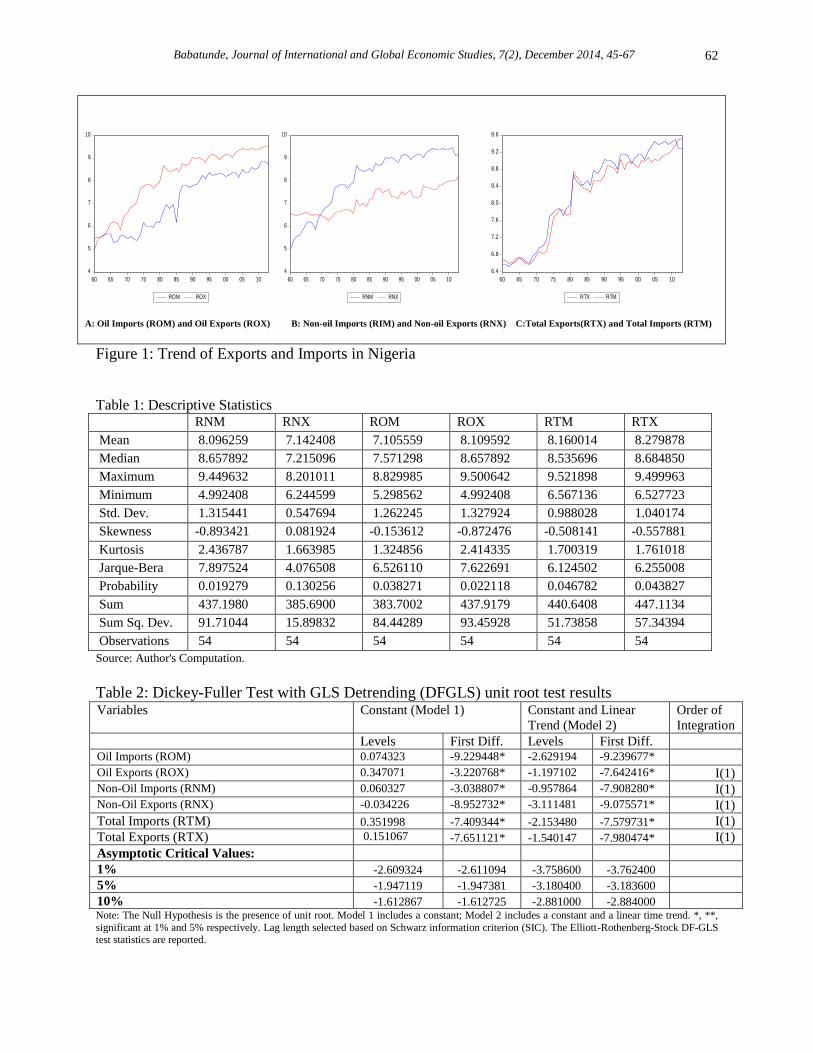
Figure 1 presents the graphical illustration of exports and imports. It is glaring that while exports

and imports drift apart at the disaggregated level (Panels A and B in Figure 1)), they have a

tendency to track each other and converge at the aggregate level (Panel C in Figure 1). While oil

exports have consistently been higher than oil imports, non-oil imports were higher than non-oil

exports. The aggregate exports and imports however showed a close relationship between

exports and imports.

The descriptive statistics of the variables is presented in Table 1. It provides information about

the means and standard deviations of the exports and imports variables. The mean value of the

logarithm of total exports and imports are at 8.27 and 8.16 respectively while the mean of the log

of oil exports stood at 8.10. Oil imports however the lowest mean logarithm value has at 7.10.

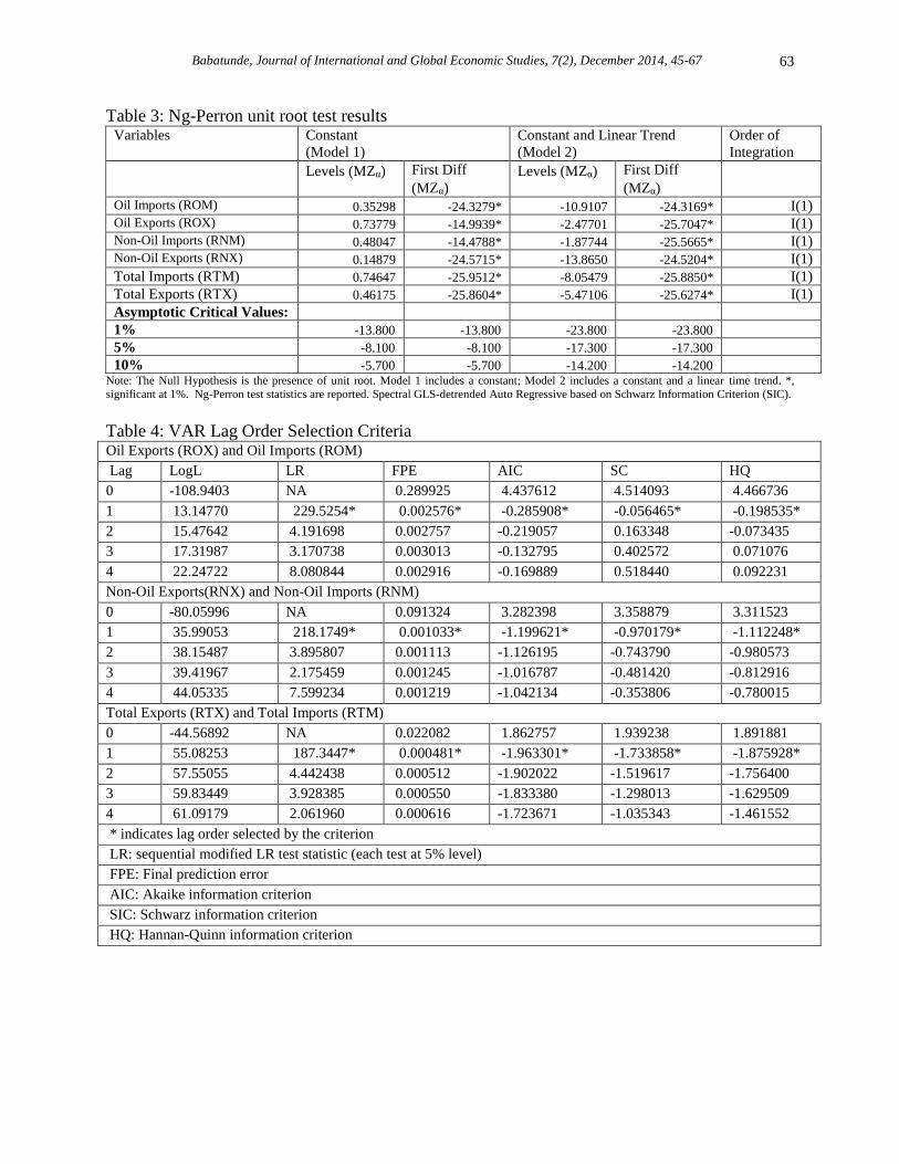
The study applies the Dickey-Fuller GLS and the Ng-Perron tests to test the order of integration

at level and first difference of the variables. For ease of result presentation and interpretation, we

present only the result of the modified forms of Phillips-Perron MZ statistics. According to the

unit root tests in Tables 2 and 3, exports and imports are integrated of order one (I (1)). Total

exports and imports in Nigeria are non-stationary at their levels but stationary at their first

difference. Also, the disaggregated variables (oil exports, oil imports, non-oil exports and non-oil

imports) were all stationary at the first difference during the period of analysis. Hence, the

assumption that the series are stationary is rejected. The results of unit test of this study

contradict Tang (2006) which found the logarithm value of export to be stationary at level and

logarithm value of import to be stationary at the first difference. Tang (2006) therefore could not

proceed with cointegration. The divergence in the result can be attributed to the Lanne,

Lutkepohl and Saikkonen (2002) and the Saikkonen and Lutkepohl (2002) unit root tests adopted

by Tang which are sensitive to the choice of the lag length chosen.

Prior to the test for cointegration, we first determine the lag length of the estimation which must

be small enough to allow estimation and high enough to ensure that errors are approximately

white noise. The lag length selection procedure is based on five different information criteria:

AIC, SIC, HQ, FPE and LR. The five information criteria in Table 4 conclude that the optimal

lag length criteria for the oil, non-oil and the aggregate exports and imports model is one. The


uniformity of the conclusions from the Information Criteria is worthy of note due to the

sensitivity of the Johansen procedure to lag length selection.

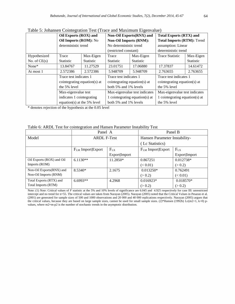
In order to determine the existence of long run relationship between the variables, the study

conducts three types of cointegration tests. These include the Johansen cointegration tests, the

Bounds test and the Hansen parameter instability test. The results of Johansen cointegration test

is reported in Table 5. The results indicate that the null hypothesis of no cointegrating vector is

rejected against the alternative hypothesis both by the trace statistics and maximum eigenvalue

statistic at 5% and 1% significance level for the aggregate exports and imports (linear

deterministic trend in the cointegrating equation and test VAR), non-oil exports and imports (no

deterministic trend and restricted constant in the cointegrating equation and test VAR) and oil

exports and imports (no deterministic trend in the cointegrating equation and test VAR). This

implies that there is positive and significant long run relationship at the one and five percent

level, implying that a common trend exists between exports and imports and export at the

aggregate and disaggregated level.

Given the inconclusive findings from the literature with respect to the existence of cointegration

between exports and imports, the study made use of exports and imports as both dependent and

independent variables in the aggregate and disaggregated model. This because of the likely

sensitivity of the choice of the dependent variable in the test for cointegration that requires the

specification of dependent and independent variable.

The ARDL model is presented in Panel A of Table 6. We first report the cointegration of exports

and imports using imports as the dependent variable following the approach of Arize (2002). For

the three models — aggregate exports and imports model, oil exports and imports model and the

non-oil exports and imports model — the calculated F-statistics are higher than the critical

values of 6.045 and 4.925 at the 5% and 10% level. Hence, we reject the null hypothesis of no

cointegration, and accept the alternative hypothesis of cointegration between exports and imports

using imports as the dependent variable.

The result was however mixed when export was used as the dependent variable following the

approach of Husted (1992). Only the disaggregated oil export and import model revealed the

existence of cointegration at the 1% level of significance. This implies that we cannot reject the

null hypothesis of cointegration for the non-oil export and import model as well as the aggregate

export and import model. This finding reinforces our initial insight on the sensitivity of the result

to the choice of the dependent variable in the investigation of the long run relationship between

exports and imports.

In order to test for the robustness of the bounds test for cointegration, Panel B of Table 6 reports

the Hansen parameter instability test of cointegration. Hansen (1992) outlines a test of the null

hypothesis of cointegration against the alternative of no cointegration. He notes that under the


alternative hypothesis of no cointegration, one should expect to see evidence of parameter

instability. Hansen proposes the use of the Lc test statistic, which arises from the theory of

Lagrange Multiplier tests for parameter instability (Hussein, 2014). Analogous to the ARDL

model, we first used imports as the dependent variable and exports as the explanatory variable.

The Lc test results did not reject the null hypothesis that oil exports and oil imports are

cointegrated at conventional levels for Nigeria when oil imports is used as the dependent

variable. However, the Lc test results was able to reject the null hypothesis of no cointegration

for the non-oil exports and imports model and the aggregate exports and imports model for

Nigeria when non-oil imports and aggregate imports were respectively used as dependent

variables. The choice of exports as the dependent variable confirmed our findings with respect to

the ARDL model on the sensitivity of the choice of variable between exports and imports. The

Lc test results did not reject the null hypothesis of cointegration in the non-oil exports and

imports model. However, the Lc tests results revealed the existence of cointegration in the oil

exports and imports model and the aggregate exports and imports model when exports was used

as the dependent variable (Panel B, Table 6).

We can therefore conclude that there is a long run relationship between exports and imports in

Nigeria at both the aggregate and disaggregated level (oil exports and imports; non-oil exports

and imports). However, for tests of cointegration that requires model specification, the choice of

the dependent variable between exports and imports is a fundamental factor that influences the

direction of the result. Thus, the existence of cointegration is partilly dependent on the

specification of the cointegration equation. Nevertheless, the existence of cointegration

relationship for the case of Nigeria implies that Nigeria is not in violation of its international

budget constraints and macroeconomic policies have been effective in bringing exports and

imports at the aggregate and disaggregated level into a long-run equilibrium.

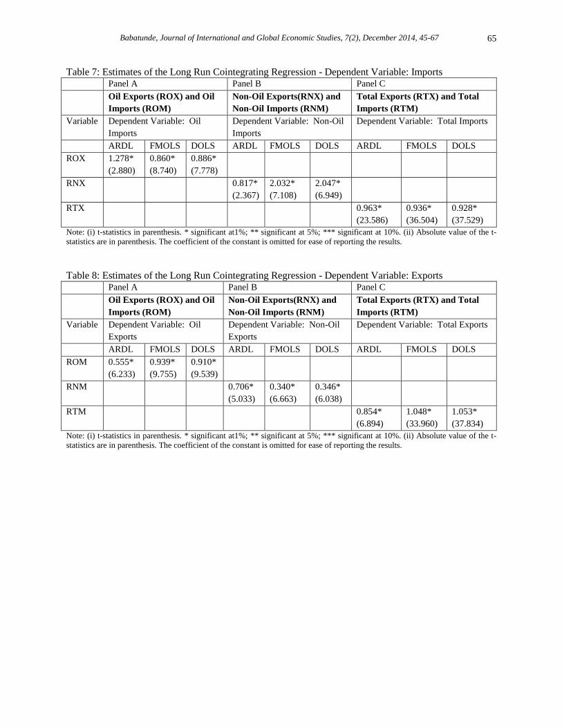
Table 7 also provides long-run estimates based on auto-regressive distributed lag ARDL

(Schwarz Bayesian Criterion) and two other long-run estimators: Fully Modified Fully Modified

Ordinary Least Square (FMOLS) and the dynamic Ordinary Least Square (DOLS). The results of

the three approaches of long-run estimates are all positive, statistically significant, and very

similar for the three models (oil exports and imports, non-oil exports and imports, and aggregate

exports and imports) demonstrating the robustness of the results. In Table 7, the estimate of the

slope coefficients for the aggregate exports and imports model were very close to unity for the

ARDL, FMOLS and the DOLS. This is an indication that in the long run one Naira of imports is

matched by one naira of exports, resulting in a long-run trade balance as well as a current

account balance. Comparably, the ARDL for the oil exports and imports model revealed a slope

coefficient of 1.278 while the FMOLS and the DOLS in the non-oil exports and imports model

revealed slope coefficients of above 2.0.


However, in Table 8 when export was adopted as the dependent variable, the ARDL reported

lower long run coefficients. Slope coefficients that were close to unity and slightly above unity

were reported in the case of oil exports and imports model and the aggregate exports and imports

model for the FMOLS and the DOLS. This confirmed the robustness of our initial result that the

choice of the dependent variable influences the direction of results in the exports and imports

estimation.

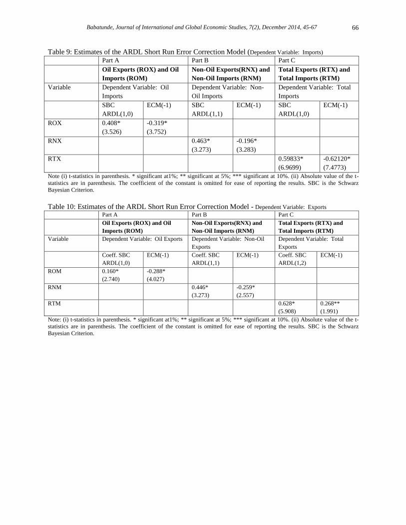
Nevertheless, the ARDL short run error correction model presented in Tables 9 (imports as

dependent variable) and 10 (exports as dependent variable) indicated that short-run imbalances

do occur since exports and imports may drift apart in the short-run. However, these short run

imbalances are temporary and appear to be sustainable in the long run given the cointegration

results reported earlier. The estimates of the error correction term for the ARDL results are also

reported in Tables 9 and 10. They all bear the expected negative sign and are significant. This

helps strengthen the findings of the long run relationship as reported by the bound test F-test. In

summary, it is evident from the various methods of cointegration that Nigeria obeys the rules of

its inter-temporal international budget constraint, i.e., existence of cointegration between export

and import. The existence of cointegration between exports and imports is similar to the findings

of Bahmani-Oskoee (1994) for Australia, Çelik (2011) for Turkey, Ali (2013) for Pakistan, Al-

Khulaifi (2013) for Qatar, Pillay (2014) for South Africa. However, it diverges from the work of

Konya and Singh (2008) for India and Dumitriu et al (2009) for Romania. They could not find

long run relationship between exports and imports respectively. Perhaps, the divergence can be

attributed to the specification error of using exports as the dependent variable.

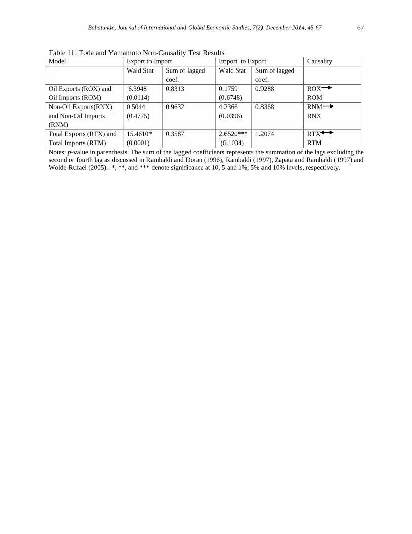
The Toda and Yamamoto granger non-causality test is reported in Table 11. The results revealed

that we can reject the null hypothesis that exports does not cause imports at 1% level of

significance. Also, we can reject the null hypothesis that imports do not cause exports at the 10%

level of significance. Thus, we can conclude that there is a bi-directional direction of causality

between aggregate exports and imports in Nigeria. This implies that there is a simultaneous

cause and effect between imports and exports in Nigeria. Our finding is consistent with the

works of Dumitriu et al (2009) for Romania, Mukhtar and Rasheed (2010) for Pakistan, and

Mohamed et al (2014) for Tunisia.

However, the non-causality tests result for the disaggregated model revealed a uni-directional

result. Oil export was found to cause oil imports while non-oil imports causes non-oil exports.

The explanation can be situated in the dominance of oil export in the Nigerian economy.

Revenue from crude oil export accounts for over 80% of government revenue, and 95% of

foreign exchange earnings. However, the mass of the crude oil extracted by the multinational oil

companies in Nigeria is refined overseas and brought back into the country as oil imports. In

addition, Nigeria is still heavily relying on the imports of items, good and services to promote the

development of its exports sector. The driver of the bi-directional causality at the aggregate level


is therefore clear. Oil exports components drives the oil imports, while non-oil imports causes

non-oil exports. It is therefore the combine effects of these interactions that established the bi-

directional causality between exports and imports in Nigeria.

5. Conclusion

The rationale of this paper was to conjecture the performance of the Nigerian trade balance and

current account. Our main concern was to investigate the long run relationship between exports

and imports in Nigeria at the aggregate and disaggregated level given the sensitivity of the

choice of the dependent variable in determining the long run relationship. As a result, the

Johansen cointegration test, the bound testing and the Hansen parameter instability test were

employed using annual data between 1960 and 2013. While the results indicate the existence of

long run relationship between exports and imports, the choice of the dependent variable between

exports and imports in the case of cointegration tests that requires the specification of dependent

and independent variables matter for the existence of long run relationship.1 However, for

cointegration models that require variable ordering, the order of the variables did not count up in

the determination of long run relationship. In specific terms, adopting imports as the dependent

variable as suggested by Arize (2002) yields a better cointegrating relationship than the Husted

(1992) framework that utilized exports as dependent variable.

While the empirical evidence revealed short-run imbalances due to the drifting apart of exports

and imports, the value of the long run coefficients were found to be close to unity. The result

implies that Nigeria is not in violation of its inter-temporal budget constraint and Nigerian trade

deficit is a short-run phenomenon but sustainable in the long-run. In addition, Nigeria's

macroeconomic policies have been quite effective to make imports and exports converge toward

equilibrium in the long-run. Finally, the Toda and Yamamoto non-causality test indicated

bidirectional causality between exports and imports. However, the different levels of significance

at the disaggregated level suggest that the influence of oil exports over oil imports is much

higher than the impact of non-oil imports over non-oil exports. The policy lesson is that the

Nigerian policy makers should make effort to diversify the economy from oil exports to non-oil

exports since shocks to the price of crude oil in the international market can affect the economy

adversely. In addition, the dependence of production on imported input should be reduced in

Nigeria. Substantial efforts should be made to produce non-oil export products which have high

domestic value added.

End Notes

*Musibau Adetunji Babatunde, Department of Economics, University of Ibadan, Ibadan,

Nigeria. E-mail: [email protected], [email protected].

1. The Bounds testing and Hansen parameter instability test requires model specification while

the Johansen cointegration requires only variable ordering.


References

Ali, S. 2013. Cointegration Analysis of Exports and Imports: The Case of Pakistan Economy.

MPRA Paper No. 49295.

Alias, E., A. Baharom, A. Radam and I. AIsmail. 2009. Trade sustainability in the forestry

domain: The case of Malaysia. Asian Social Science, 5(12): 78-83.

Al-Khulaifi, A.S. 2013. Exports and Imports in Qatar: Evidence From Cointegration and Error

Correction Model. Asian Economic and Financial Review, 3(9):1122-1133.

Arize, A.C. 2002. Imports and Exports in 50 Countries: Tests of Cointegration and Structural

Breaks, International Review of Economics and Finance, vol. 11, pp. 101- 115.

Baharumshah, A.Z., Lau, E., S. Fountas. 2003. On The Sustainability Of Current Account

Deficits: Evidence From Four ASEAN Countries. Journal of Asian Economics, 14, 465-

487,doi:10.1016/s1049-0078(03)00038-1,http://dx.doi.org/10.1016/S1049

0078(03)00038-1.

Bahmani-Oskooee, M. 1994. Are Imports and Exports of Australia Cointegrated? Journal of

Economic Integration, 9(4), 525-533.

Bahmani-Oskooee, M. and H.-R. Ree. 1997. Are Imports and Exports of Korea Cointegrated?

International Economic Journal, vol. 11, pp. 109-114.

Çelik, T. 2011. Long Run Relationship Between Export and Import: Evidence from Turkey for

the period of 1990-2010. International Conference On Applied Economics – ICOAE

Cheong, T.T. 2005. Are Malaysian Exports and Imports Cointegrated? A Comment. Sunway

Academic Journal 2, 101–107.

Dolado, J. J. and H. Lutkepohl. 1996. Making Wald tests work for Cointegrated VAR

systems, Econometric Review, 15, 369–86.

Dumitriu, R., R Stefanescu and C. Nistor. 2009. Cointegration And Causality Between

Romanian Exports And Imports. “Dunarea de Jos” University Galati, Faculty of

Economic Sciences.

Emmy, F.A., A.H. Baharom, A. Radam and I. Illisriyani. 2009. Export and Import

Cointegration in Forestry Domain: The Case of Malaysia. MPRA Paper No. 16673.

Fountas, S., and Wu, J. L. 1999. Are The US Current Account Deficits Really Sustainable?

International Economic Journal, 13, 51-58.

Gregory, A.W., and B. E. Hansen. 1996. Residual-Based Tests for Cointegration in Models

with Regime Shifts.” Journal of Econometrics 70 (1996): 99-126.

Halicioglu, F. 2007. A multivariate causality analysis of export and growth for Turkey, MPRA

Paper 3565, University Library of Munich, Germany.

Herzer, D. and D.F. Nowak-Lehman. 2006. Is There a Long-Run Relationship Between

Exports and Imports in Chile? Applied Economics Letters, vol. 13, pp. 981-986.

Hussein, J. 2014. Are Exports And Imports Cointegrated? Evidence From Nine MENA

Countries. Applied Econometrics and International Development Vol. 14-1.

Husted, S. 1992. The Emerging U.S. Current Account Deficit in the 1980s: A Cointegration

Analysis, Review of Economics and Statistics, vol. 74, pp. 159-166.

Husted, S. 1992. The Emerging U.S. Current Account Deficit in the 1980s: A Cointegration

Analysis, Review of Economics and Statistics, vol. 74, pp. 159-166.

Hye, Q.M. and M.M Siddiqui. 2010. Are Imports and Exports Cointegrated in Pakistan? A

Rolling Window Bound Testing Approach. World Applied Sciences Journal, 9(7), 708-

711.


Irandoust, M., and J. Ericsson. 2004. Are Imports and Exports Cointegrated? An

International Comparison. Metroeconomica, 55 (1), 49-64.

Jiranyakul, K. 2012. Are Thai manufacturing exports and imports of capital goods related? .

Modern Economy, 3: 237-244.

Johansen, S. and K. Juselius. 1990. Maximum likelihood estimation and inference on

cointegration: with applications to the demand for money, Oxford Bulletin of Economics

and Statistics, 52, 169–210.

Johansen, S. 1991. Estimation and hypothesis testing of cointegration vectors in gaussian

vector autoregressive models. Econometrica, 59 (6), 1551-1580.

Keong, C. C., Soo, S. C., and Y. Zulkornain. 2004. Are Malaysian Exports and Imports

Cointegrated? Sunway College Journal 1, 29-38.

Konya, L., and J.P. Singh. (2008) Are Indian Exports And Imports Cointegrated? Applied

Econometrics and International Development Vol- 8-2.

Lanne, M., H. Lutkepohl, and P. Saikkonen. 2002. Comparison of Unit Root Tests for Time

Series with Level Shifts. Journal of Time Series Analysis 23, no. 6, 667-85.

Lanne, M., H. Lutkepohl, and P. Saikkonen. 2003. Test Procedures for Unit Roots in Time

Series with Level Shifts at Unknown Time. Oxford Bulletin of Economics and Statistics

65, no. 1, 91-115.

Mohamed, M.B.H, S. Saafi and A. Farhat. 2014. Testing the Causal Relationship Between

Exports and Imports Using a Toda and Yamamoto Approach. Evidence From Tunisia.

International Conference on Business 2, 75-80.

Mukhtar, T. and S. Rasheed. 2010. Testing Long Run Relationship between Exports and

Imports: Evidence from Pakistan. Journal of Economic Cooperation and Development

31(1), 41-58.

Narayan, P. K. 2005. The saving and investment nexus for China: evidence from cointegration

tests, Applied Economics, 37, 1979–90.

Pillay, S. 2014. The Long Run Relationship between Exports and Imports in South Africa:

Evidence from Cointegration Analysis. World Academy of Science, Engineering and

Technology International Journal of Social, Management, Economics and Business

Engineering Vol:8 No:6.

Rammadhan, M. and A. Naseeb. 2008. The long-run relationship between oil exports and

aggregate imports in the gcc: Cointegration analysis. Journal of Economic Cooperation,

29(2): 69-84.

Tang, T. C. 2006. Are imports and exports in the OIC member countries cointegrated? A re-

examination. IIUM Journal of Economics and Management. 14 (1), 1-31.

Tang, T.C. and A.H. Mohammad. 2005. Are imports and exports of oic countries cointegrated?

An empirical study. Labuan Bulletin of International Business and Finance, 3: 33-47.

Toda, H. Y. and P. Phillips 1993. Vector auto regressions and causality, Econometrica, 61,

1367–93.

Toda, H. Y. and T. Yamamoto 1995. Statistical inference in vector autoregression with

possibly integrated processes, Journal of Econometrics, 66, 225–50.

Tsen, W. 2006. Granger causality tests among openness to international trade, human capital

accumulation and economic growth in China: 1952–1999, International Economic

Journal, Korean International Economic Association, 20, 285–302.


Uddin, J. 2009. Time Series Behaviour of Imports and Exports of Bangladesh Evidence from

Cointegration Analysis and Error Correction Model. International Journal of Economics

and Finance 1(2), 156-162.

Zapata, H. O. and A. N.Rambaldi.1997. Monte Carlo evidence on cointegration and

causation, Oxford Bulletin of Economics and Statistics, 59, 285–98.


4

5

6

7

8

9

10

60 65 70 75 80 85 90 95 00 05 10

ROM ROX

4

5

6

7

8

9

10

60 65 70 75 80 85 90 95 00 05 10

RNM RNX

6.4

6.8

7.2

7.6

8.0

8.4

8.8

9.2

9.6

60 65 70 75 80 85 90 95 00 05 10

RTX RTM

A: Oil Imports (ROM) and Oil Exports (ROX) B: Non-oil Imports (RIM) and Non-oil Exports (RNX) C:Total Exports(RTX) and Total Imports (RTM)

Figure 1: Trend of Exports and Imports in Nigeria

Table 1: Descriptive Statistics RNM RNX ROM ROX RTM RTX

Mean 8.096259 7.142408 7.105559 8.109592 8.160014 8.279878

Median 8.657892 7.215096 7.571298 8.657892 8.535696 8.684850

Maximum 9.449632 8.201011 8.829985 9.500642 9.521898 9.499963

Minimum 4.992408 6.244599 5.298562 4.992408 6.567136 6.527723

Std. Dev. 1.315441 0.547694 1.262245 1.327924 0.988028 1.040174

Skewness -0.893421 0.081924 -0.153612 -0.872476 -0.508141 -0.557881

Kurtosis 2.436787 1.663985 1.324856 2.414335 1.700319 1.761018

Jarque-Bera 7.897524 4.076508 6.526110 7.622691 6.124502 6.255008

Probability 0.019279 0.130256 0.038271 0.022118 0.046782 0.043827

Sum 437.1980 385.6900 383.7002 437.9179 440.6408 447.1134

Sum Sq. Dev. 91.71044 15.89832 84.44289 93.45928 51.73858 57.34394

Observations 54 54 54 54 54 54

Source: Author's Computation.

Table 2: Dickey-Fuller Test with GLS Detrending (DFGLS) unit root test results Variables Constant (Model 1) Constant and Linear

Trend (Model 2)

Order of

Integration

Levels First Diff. Levels First Diff. Oil Imports (ROM) 0.074323 -9.229448* -2.629194 -9.239677* Oil Exports (ROX) 0.347071 -3.220768* -1.197102 -7.642416* I(1) Non-Oil Imports (RNM) 0.060327 -3.038807* -0.957864 -7.908280* I(1) Non-Oil Exports (RNX) -0.034226 -8.952732* -3.111481 -9.075571* I(1)

Total Imports (RTM) 0.351998 -7.409344* -2.153480 -7.579731* I(1)

Total Exports (RTX) 0.151067 -7.651121* -1.540147 -7.980474* I(1)

Asymptotic Critical Values:

1% -2.609324 -2.611094 -3.758600 -3.762400

5% -1.947119 -1.947381 -3.180400 -3.183600

10% -1.612867 -1.612725 -2.881000 -2.884000 Note: The Null Hypothesis is the presence of unit root. Model 1 includes a constant; Model 2 includes a constant and a linear time trend. *, **,

significant at 1% and 5% respectively. Lag length selected based on Schwarz information criterion (SIC). The Elliott-Rothenberg-Stock DF-GLS test statistics are reported.


Table 3: Ng-Perron unit root test results Variables Constant

(Model 1)

Constant and Linear Trend

(Model 2)

Order of

Integration

Levels (MZα) First Diff

(MZα)

Levels (MZα) First Diff

(MZα)

Oil Imports (ROM) 0.35298 -24.3279* -10.9107 -24.3169* I(1) Oil Exports (ROX) 0.73779 -14.9939* -2.47701 -25.7047* I(1) Non-Oil Imports (RNM) 0.48047 -14.4788* -1.87744 -25.5665* I(1) Non-Oil Exports (RNX) 0.14879 -24.5715* -13.8650 -24.5204* I(1)

Total Imports (RTM) 0.74647 -25.9512* -8.05479 -25.8850* I(1)

Total Exports (RTX) 0.46175 -25.8604* -5.47106 -25.6274* I(1)

Asymptotic Critical Values:

1% -13.800 -13.800 -23.800 -23.800

5% -8.100 -8.100 -17.300 -17.300

10% -5.700 -5.700 -14.200 -14.200 Note: The Null Hypothesis is the presence of unit root. Model 1 includes a constant; Model 2 includes a constant and a linear time trend. *,

significant at 1%. Ng-Perron test statistics are reported. Spectral GLS-detrended Auto Regressive based on Schwarz Information Criterion (SIC).

Table 4: VAR Lag Order Selection Criteria Oil Exports (ROX) and Oil Imports (ROM)

Lag LogL LR FPE AIC SC HQ

0 -108.9403 NA 0.289925 4.437612 4.514093 4.466736

1 13.14770 229.5254* 0.002576* -0.285908* -0.056465* -0.198535*

2 15.47642 4.191698 0.002757 -0.219057 0.163348 -0.073435

3 17.31987 3.170738 0.003013 -0.132795 0.402572 0.071076

4 22.24722 8.080844 0.002916 -0.169889 0.518440 0.092231

Non-Oil Exports(RNX) and Non-Oil Imports (RNM)

0 -80.05996 NA 0.091324 3.282398 3.358879 3.311523

1 35.99053 218.1749* 0.001033* -1.199621* -0.970179* -1.112248*

2 38.15487 3.895807 0.001113 -1.126195 -0.743790 -0.980573

3 39.41967 2.175459 0.001245 -1.016787 -0.481420 -0.812916

4 44.05335 7.599234 0.001219 -1.042134 -0.353806 -0.780015

Total Exports (RTX) and Total Imports (RTM)

0 -44.56892 NA 0.022082 1.862757 1.939238 1.891881

1 55.08253 187.3447* 0.000481* -1.963301* -1.733858* -1.875928*

2 57.55055 4.442438 0.000512 -1.902022 -1.519617 -1.756400

3 59.83449 3.928385 0.000550 -1.833380 -1.298013 -1.629509

4 61.09179 2.061960 0.000616 -1.723671 -1.035343 -1.461552

* indicates lag order selected by the criterion

LR: sequential modified LR test statistic (each test at 5% level)

FPE: Final prediction error

AIC: Akaike information criterion

SIC: Schwarz information criterion

HQ: Hannan-Quinn information criterion


Table 5: Johansen Cointegration Test (Trace and Maximum Eigenvalue) Oil Exports (ROX) and

Oil Imports (ROM): No

deterministic trend

Non-Oil Exports(RNX) and

Non-Oil Imports (RNM):

No deterministic trend

(restricted constant)

Total Exports (RTX) and

Total Imports (RTM): Trend

assumption: Linear

deterministic trend

Hypothesized

No. of CE(s)

Trace

Statistic

Max-Eigen

Statistic

Trace

Statistic

Max-Eigen

Statistic

Trace Statistic Max-Eigen

Statistic

None* 13.84767 11.27529 23.01751 17.06880 17.37837 14.61472

At most 1 2.572386 2.572386 5.948709 5.948709 2.763655 2.763655

Trace test indicates 1

cointegrating equation(s) at

the 5% level



both 5% and 1% levels



the 5% level

Max-eigenvalue test

indicates 1 cointegrating

equation(s) at the 5% level

Max-eigenvalue test indicates

1 cointegrating equation(s) at

both 5% and 1% levels

Max-eigenvalue test indicates

1 cointegrating equation(s) at

the 5% level

* denotes rejection of the hypothesis at the 0.05 level

Table 6: ARDL Test for cointegration and Hansen Parameter Instability Test

Panel A Panel B

Model ARDL F-Test Hansen Parameter Instability-

( Lc Statistics)

FLM Import|Export FLX

Export|Import

FLM Import|Export FLX

Export|Import

Oil Exports (ROX) and Oil

Imports (ROM) 6.1130** 11.2850* 0.867251

(< 0.01)

0.012738*

(> 0.2)


Non-Oil Imports (RNM) 8.5340* 2.1675 0.013250*

(> 0.2)

0.762491

(< 0.01)


Total Imports (RTM)

6.6993** 4.2968 0.016923*

(> 0.2)

0.018570*

(> 0.2)

Note: (1) Note: Critical values of F statistic at the 5% and 10% levels of significance are 6.045 and 4.925 respectively for case III: unrestricted

intercept and no trend for n=55. The critical values are taken from Narayan (2005). Narayan (2005) noted that the Critical Values in Pesaran et al.

(2001) are generated for sample sizes of 500 and 1000 observations and 20 000 and 40 000 replications respectively. Narayan (2005) argues that the critical values, because they are based on large sample sizes, cannot be used for small sample sizes. (2)*Hansen (1992b) Lc(m2=1, k=0) p-

values, where m2=m-p2 is the number of stochastic trends in the asymptotic distribution.


Table 7: Estimates of the Long Run Cointegrating Regression - Dependent Variable: Imports Panel A Panel B Panel C


Imports (ROM)


Non-Oil Imports (RNM)

Total Exports (RTX) and Total

Imports (RTM)

Variable Dependent Variable: Oil

Imports

Dependent Variable: Non-Oil

Imports

Dependent Variable: Total Imports

ARDL FMOLS DOLS ARDL FMOLS DOLS ARDL FMOLS DOLS

ROX 1.278*

(2.880)

0.860*

(8.740)

0.886*

(7.778)

RNX

0.817*

(2.367)

2.032*

(7.108)

2.047*

(6.949)

RTX

0.963*

(23.586)

0.936*

(36.504)

0.928*

(37.529)

Note: (i) t-statistics in parenthesis. * significant at1%; ** significant at 5%; *** significant at 10%. (ii) Absolute value of the t-

statistics are in parenthesis. The coefficient of the constant is omitted for ease of reporting the results.

Table 8: Estimates of the Long Run Cointegrating Regression - Dependent Variable: Exports Panel A Panel B Panel C


Imports (ROM)



Total Exports (RTX) and Total

Imports (RTM)


Exports

Dependent Variable: Non-Oil

Exports

Dependent Variable: Total Exports

ARDL FMOLS DOLS ARDL FMOLS DOLS ARDL FMOLS DOLS

ROM 0.555*

(6.233)

0.939*

(9.755)

0.910*

(9.539)

RNM

0.706*

(5.033)

0.340*

(6.663)

0.346*

(6.038)

RTM

0.854*

(6.894)

1.048*

(33.960)

1.053*

(37.834)


statistics are in parenthesis. The coefficient of the constant is omitted for ease of reporting the results.


Table 9: Estimates of the ARDL Short Run Error Correction Model (Dependent Variable: Imports) Part A Part B Part C


Imports (ROM)




Total Imports (RTM)


Imports

Dependent Variable: Non-

Oil Imports

Dependent Variable: Total

Imports

SBC

ARDL(1,0)

ECM(-1) SBC

ARDL(1,1)

ECM(-1) SBC

ARDL(1,0)

ECM(-1)

ROX 0.408*

(3.526)

-0.319*

(3.752)

RNX

0.463*

(3.273)

-0.196*

(3.283)

RTX

0.59833*

(6.9699)

-0.62120*

(7.4773)

Note (i) t-statistics in parenthesis. * significant at1%; ** significant at 5%; *** significant at 10%. (ii) Absolute value of the t-

statistics are in parenthesis. The coefficient of the constant is omitted for ease of reporting the results. SBC is the Schwarz

Bayesian Criterion.

Table 10: Estimates of the ARDL Short Run Error Correction Model - Dependent Variable: Exports Part A Part B Part C


Imports (ROM)




Total Imports (RTM)

Variable Dependent Variable: Oil Exports Dependent Variable: Non-Oil

Exports

Dependent Variable: Total

Exports

Coeff. SBC

ARDL(1,0)

ECM(-1) Coeff. SBC

ARDL(1,1)

ECM(-1) Coeff. SBC

ARDL(1,2)

ECM(-1)

ROM 0.160*

(2.740)

-0.288*

(4.027)

RNM

0.446*

(3.273)

-0.259*

(2.557) RTM

0.628*

(5.908)

0.268**

(1.991)


statistics are in parenthesis. The coefficient of the constant is omitted for ease of reporting the results. SBC is the Schwarz

Bayesian Criterion.


Table 11: Toda and Yamamoto Non-Causality Test Results Model Export to Import Import to Export Causality

Wald Stat Sum of lagged

coef.

Wald Stat Sum of lagged

coef.

Oil Exports (ROX) and

Oil Imports (ROM)

6.3948

(0.0114)

0.8313 0.1759

(0.6748)

0.9288 ROX

ROM

Non-Oil Exports(RNX)

and Non-Oil Imports

(RNM)

0.5044

(0.4775)

0.9632 4.2366

(0.0396)

0.8368 RNM

RNX


Total Imports (RTM)

15.4610*

(0.0001)

0.3587 2.6520***

(0.1034)

1.2074 RTX

RTM

Notes: p-value in parenthesis. The sum of the lagged coefficients represents the summation of the lags excluding the

second or fourth lag as discussed in Rambaldi and Doran (1996), Rambaldi (1997), Zapata and Rambaldi (1997) and

Wolde-Rufael (2005). *, **, and *** denote significance at 10, 5 and 1%, 5% and 10% levels, respectively.

Are Exports and Imports Cointegrated DEC 2014...Are Exports and Imports Cointegrated? ......

Documents

Transcript of Are Exports and Imports Cointegrated DEC 2014...Are Exports and Imports Cointegrated? ......