establish Subgrade Support Values For Typicaltransctr/pdf/netc/netcr57_02-3.pdf · ESTABLISH...

ESTABLISH SUBGRADE SUPPORT VALUES FOR TYPICAL SOILS IN NEW ENGLAND

By

Dr. Ramesh B. Malla, PI

and Ms. Shraddha Joshi, Graduate Research Assistant

Prepared for The New England Transportation Consortium

April 10, 2006

NETCR 57 Project No. 02-3

This report, prepared in cooperation with the New England Transportation Consortium, does not constitute a standard, specification, or regulation. The contents of this report reflect the views of the authors who are responsible for the facts and the accuracy of the data presented herein. The contents do not necessarily reflect the views of the New England Transportation Consortium or

the Federal Highway Administration.

ii

Technical Report Documentation Page

1. Report No. NETCR 57

2. Government Accession No.

N/A 3. Recipient’s Catalog No.

N/A

4. Title and Subtitle

5. Report Date

April 10, 2006

6. Performing Organization Code

N/A 7. Author(s) 8. Performing Organization Report No.

Ramesh B. Malla, Ph.D., Associate Professor (PI) and Shraddha Joshi, Graduate Research Assistant

NETCR 57

9. Performing Organization Name and Address 10 Work Unit No. (TRAIS)

University of Connecticut Department of Civil and Environmental Engineering 261 Glenbrook Road, Storrs, CT 06269-2037

N/A

11. Contract or Grant No.

N/A 13. Type of Report and Period Covered 12. Sponsoring Agency Name and Address

New England Transportation Consortium C/o Advanced Technology & Manufacturing Center University of Massachusetts Dartmouth 151 Martine Street Fall River, MA 02723

FINAL REPORT

14. Sponsoring Agency Code

NETC 02-3. A study conducted in cooperation with the U.S. DOT

15 Supplementary Notes

N/A 16. Abstract

17. Key Words

Resilient Modulus, Subgrade, AASHTO soil types, Regression, Prediction Models, Falling Weight Deflectometer, Backcalculated modulus.

18. Distribution Statement

No restrictions. This document is available to the public through the National Technical Information Service, Springfield, Virginia 22161.

19. Security Classif. (of this report) Unclassified

20. Security Classif. (of this page) Unclassified

21. No. of Pages

22. Price

N/A Form DOT F 1700.7 (8-72) Reproduction of completed page authorized

Establish Subgrade Support values for Typical Soils in New England

The main objective of this research project was to establish prediction models for subgrade support (resilient modulus, MR) values for typical soils in New England. This soil strength property can be measured in the laboratory by means of repeated load triaxial tests. Non-destructive tests like Falling Weight Deflectometer (FWD) can be used to estimate the modulus value using backcalculation process. The current study used data extracted from Long Term Pavement Performance Information Management System (LTPP IMS) Database for 300 test specimens from 19 states in New England and nearby regions in the U.S. and 2 provinces in Canada. Prediction equations were developed using SAS® for six AASHTO soil types viz. A-1-b, A-3, A-2-4, A-4, A-6, and A-7-6 and USCS soil types Coarse Grained Soils and Fine Grained Soils found in New England region to estimate resilient modulus. To verify the prediction models, MR values for 5 types of soils in New England were determined from laboratory testing using AASHTO standards. The predicted and laboratory measured MR values matched reasonably well for the soils considered. Also an attempt was made to obtain relationship between laboratory MR values and FWD backcalculated modulus from the LTPP test data. No definitive conclusion could be drawn from the analysis. However, in general, FWD backcalculated modulus values were observed to be greater than the laboratory determined modulus values for the same soil type.

iv

ESTABLISH SUBGRADE SUPPORT VALUES FOR TYPICAL SOILS IN NEW ENGLAND

Ramesh B. Malla, Ph.D., Associate Professor (Principal Investigator)

and Shraddha Joshi, Graduate Research Assistant

Department of Civil and Environmental Engineering

University of Connecticut 261 Glenbrook Road, Storrs, CT 06269-2037

Prepared for

The New England Transportation Consortium

NETCR 57 Project No. 02-3

EXECUTIVE SUMMARY

The main objective of this research project was to establish prediction models for subgrade support (resilient modulus, MR) values for typical soils in New England. Resilient modulus is a definitive elastic material property of soil recognizing certain nonlinear characteristics and used to characterize roadbed soil for pavement design. This soil strength property can be measured in the laboratory by means of repeated load triaxial tests. Non-destructive tests like Falling Weight Deflectometer (FWD) can be used to estimate the modulus value using backcalculation process.

In order to identify the major soil types occurring in New England region, a thorough review

of United States Department of Agriculture (USDA) soil survey reports was conducted. The predominant soil types identified for the five New England States are: Connecticut - A-2 and A-4; Maine - A-1, A-2, A-3, A-4, A-5, and A-6; Massachusetts - A-1, A-2, A-3, A-4, A-5, and A-6; New Hampshire – A-1, A-2, and A-4; Vermont - A-1, A-2, A-4, A-6, and A-7. The predominant soil type in Rhode Island could not be identified because the soil types occurring in the entire state has been given, county wise soil types is not available.

Resilient modulus prediction models were developed for six predominant AASHTO

(American Association of State Highway and Transportation Officials) soil types (A-1-b, A-3, A-2-4, A-4, A-6, and A-7-6) found in New England using SAS®. The current study used data extracted from Long Term Pavement Performance Information Management System (LTPP IMS) Database for 300 test specimens from 19 states in New England and nearby regions in the U.S. and 2 provinces in Canada. Soil types A-1-a, A-2-5, A-2-7, A-5, and A-7-5 were not present in the test sites considered for this study. Generalized constitutive model consisting bulk stress and octahedral shear stress was used to predict the resilient modulus of subgrade soils by developing regression equations for the k coefficients that relate them to the soil properties. Three set of prediction models were developed for each soil type. The first set of models were developed from all available soil samples for a particular soil type, the second set of models were developed from only those samples that had been compacted at optimum moisture content during

v

MR test, and the third set of models were developed taking samples that had been compacted at insitu moisture content during MR test. The regression equations show that for different k coefficients, different set of soil properties have the major contribution. The R2 values obtained for the k coefficient prediction models varied from 0.30 to 0.99.

Furthermore, the data collected from the LTPP database were classified according to Unified

Soil Classification System (USCS) into Coarse Grained and Fine Grained soils and separate prediction models were developed for each of them. Two models were developed for coarse grained soils, one with all coarse grained soil samples available in LTPP database and other with only those samples that had Uniformity Coefficient (CU) less than 100. In these cases, the R2 values obtained for the k coefficient prediction models varied from 0.22 to 0.63.

The R2 values obtained in the present study are not as high as those reported in some of the

previous studies which were based on testing of a rather limited number of soil samples with controlled soil parameters and consistent laboratory environment. The soil specimens collected for tests in the LTPP program, whose results were used in this study, were from varied and wide locations. Moreover, the resilient modulus test results reported in the LTPP database were not obtained from a single laboratory so there is a possibility of error due to equipment/operator variability.

To verify the prediction models, MR values for 5 types of soils in New England were

determined from laboratory testing using AASHTO standards. The predicted and laboratory measured MR values matched reasonably well when the soil properties values for the samples were within the range of the values used in developing the prediction models.

Also an attempt was made to obtain relationship between laboratory MR values and FWD

backcalculated modulus from the LTPP test data. No definitive conclusion could be drawn from the analysis due to lack of data of these two types of tests performed under similar conditions of moisture, density, and season and field stress data. However, in general, FWD backcalculated modulus values were observed to be greater than the laboratory determined modulus values for the same soil type.

vi

ACKNOWLEDGEMENTS

The authors would like to thank New England Transportation Consortium (NETC) for sponsoring the project and providing the financial support. Special appreciation goes to the Technical Committee members of this NETC project for their valuable comments. Our special thanks to the Chair of the Technical Committee, Mr. Leo Fontaine of the Connecticut Department of Transportation for his invaluable suggestions, prompt, and timely attention to our needs, and his assistance throughout this project duration. We would like to thank Connecticut Department of Transportation (Mr. Leo Fontaine) and Vermont Agency of Transportation (Mr. Michael Pologruto and Mr. Chris Benda) for their help in the collection of soil samples used in the laboratory testing in this study. Authors are thankful to Long Term Pavement Performance (LTPP) Technical Support Services Contractor, Oak Ridge, Tennessee for providing the LTPP IMS (Information Management System) data CDs and Mr. John Rush at LTPP Customer Support for answering questions related to the LTPP database. We would like to extend our sincere thanks to Braun Intertec Corporation, Minneapolis, MN for conducting the laboratory tests of several New England soil samples to classify and determine their resilient modulus according to AASHTO standards. The authors would like to acknowledge Dr. Vincent Janoo, U.S. Army Cold Regions Research and Engineering Laboratory (CRREL), Hanover, New Hampshire for his advice and comments during the initial phase of this project. The authors also wish to recognize Mr. Umashankar Balunaini, Graduate Research Assistant on this project during the initial period of January–December 2003 for his help in doing initial literature search and data collection. Finally, the authors would like to thank the NETC program office, Connecticut Transportation Institute, and the Department of Civil & Environmental Engineering, University of Connecticut, Storrs, CT for research facilities and logistics support.

vii

TABLE OF CONTENTS

Title Page…………………………………………………………………………………... i

Technical Report Documentation Page…………………………………………………... ii

Metric Conversion Factors………………………………………………………………. iii

Executive Summary ………………………………………………………………………. iv

Acknowledgements………………………………………………………………………… vi

Table of Contents………………………..………………………………………………… vii

List of Tables…………………………………………………...…………………………. x

List of Figures…………………………………………………........................................... xiv

1. Introduction ……………………………………………………………………………. 1.1 Subgrade Resilient Modulus ……………………………………………………….. 1.2 Objectives …………………………………………………………………………. 1.3 Organization of Report ……………………………………………………………...

1 1 2 3

2. Literature Review……………………………………………………………................. 2.1 Previous Studies on Laboratory Resilient Modulus and FWD Backcalculated

Modulus in New England Region…………………………………………………... 2.2 Other studies on Laboratory Resilient Modulus……………………………………. 2.3 Other Studies on FWD Backcalculated Modulus…………………………………... 2.4 LTPP study on Laboratory Resilient Modulus and FWD Backcalculated Modulus .

4 4 6 6 7

3. Subgrade Soil Types in New England States………………………………………… 3.1 General Soil Classification Systems ……………………………………….............. 3.2 Soil Classification of New England States………………………………………….

9 9 10

4. Resilient Modulus by AASHTO Soil Types ……………………................................. 4.1 Resilient Modulus values for different AASHTO soil types from LTPP database

4.2 Variation of Resilient Modulus with Stress Levels………………………………… 4.3 Resilient Modulus Prediction Models………………………………………………

4.3.1 Generalized Constitutive Model……………………………………………… 4.3.2 Regression Analysis Methodology ………………………………................... 4.3.3 Results of Regression Analysis……………………………………………….

4.3.3.1 Soil Type: A-1-b ……………………………………………………... 4.3.3.2 Soil Type: A-3 ……………………………………………………...... 4.3.3 Soil Type: A-2-4 ……………………………………………………... 4.3.3.4 Soil Type: A-4 ……………………………………………………....... 4.3.3.5 Soil Type: A-6 ……………………………………………………....... 4.3.3.6 Soil Type: A-7-6 ……………………………………………………...

4.4 Limits of Soil Properties Values used in Second Step Regression for AASHTO Soil Types …………………………………………………………………………..

14 14 23 31 32 33 39 39 44 48 53 58 62 67

5. Resilient Modulus of Subgrades by USCS Soil Types ……………………………...... 5.1 Resilient Modulus Prediction Models for USCS Soil Types ……………………… 5.1.1 USCS Soil Type: Coarse Grained …………………………………………….

71 71 73

viii

5.1.2 USCS Soil Type: Fine Grained ……………………………………………… 5.2 Limits of Soil Properties Values used in Second Step Regression for USCS Soil

Types ……………………………………………………………………………...

78 81

6. Experimental Verification ……...………………………………………………............ 6.1 Resilient Modulus Test Procedure ………………………………………………….

6.2 Soil Samples Data Collected in New England ……………………………………... 6.3 Soil Physical Properties and Soil Classification of the Collected Soil Samples ….. 6.4 Laboratory Resilient Modulus Test Results ……………………………………….

6.5 Verification of Prediction Models developed for AASHTO Soil Types ………….. 6.5.1 Verification of Prediction Model for A-1-b Soil …………………………... 6.5.2 Verification of Prediction Model for A-3 Soil ……………………………... 6.5.3 Verification of Prediction Model for A-2-4 Soil …………………………... 6.5.4 Verification of Prediction Model for A-4 Soil ……………………………. 6.5.5 Verification of Prediction Model for A-7-6 Soil …………………………...

6.6 Verification of Prediction Models developed for USCS Soil Types ………………. 6.6.1 Verification of Prediction Model for USCS Soil Type: Coarse Grained (All

Samples) ……………………………………………………………………. 6.6.2 Verification of Prediction Model for USCS Soil Type: Coarse Grained

(Samples with CU≤100) ……………………………………………………. 6.6.3 Verification of Prediction Model for USCS Soil Type: Fine Grained ……...

82 82 83 84 86 102 103 104 107 108 110 110 111 112 114

7. Subgrade Support Values from Falling Weight Deflectometer Tests……………… 7.1 Falling Weight Deflectometer (FWD) Test and the Backcalculated Modulus …….. 7.2 Comparison of Laboratory Resilient Modulus and FWD Backcalculated Modulus .

117 117 118

8. Summary and Conclusions …………………………………...……………………… 120

9. References and Bibliography …………………………………………….................... 131

Appendices (Available in CD ROM) …………………………………………………… Appendix A - Soil Types in New England based on USDA reports …………………...

Appendix B - LTPP Test Sites for Laboratory Resilient Modulus and Falling Weight Deflectometer (FWD) Backcalculated Modulus ………………………

Appendix C - Stresses, Laboratory MR and MR calculated from Prediction Models for soil samples data extracted from LTPP database ……………………….

Appendix D – Data Used and Obtained from Regression Analysis of AASHTO Soil Types …………………………………………………………………… Appendix E – Analysis of Data Extracted from LTPP database for USCS Soil Types ..

Appendix F - Predicted Values of k Coefficients and Predicted MR for USCS Soil Types ……………………………………………………………………

Appendix G - Proctor Test and Grain Size Distribution Curves for the Soil Samples Tested …………………………………………………………………...

Appendix H – Comparison of Laboratory MR and Backcalculated MR for LTPP test sites ……………………………………………………………………..

Appendix I – Data extracted from LTPP IMS database ………………………………. Appendix I.1 – State Code, Pavement Layer and AASHTO soil classification of

subgrade information for LTPP test sites ………………………… Appendix I.2 – Laboratory Resilient Modulus Test Data …………………………

141 142 152 148 159 240 267 292 331 355 412 415 537

ix

Appendix I.3 – FWD Backcalculated Moduls Data ………………………………. Appendix I.4 – LTPP Database Quality Control Checks …………………………

787 1080

x

LIST OF TABLES

Table 1 MR for New Hampshire Subgrade Soils 5 Table 2 MR and FWD modulus for Rhode Island Subgrade Soils 5 Table 3 Summary of literatures on relationship between FWD backcalculated

and laboratory measured resilient modulus

8 Table 4 AASHTO Soil Classification System 9 Table 5 USCS Classification compared with AASHTO classification 11 Table 6 Soil types in New England States 13 Table 7 Total number of soil samples by states for which data collected from

LTPP database

15 Table 8 Number of samples by AASHTO soil types for which data was

extracted from the LTPP database

32 Table 9 Sample Laboratory MR test data (one A-2-4 soil specimen from

Connecticut) 34

Table 10 Sample stress and MR values used in first step regression 34 Table 11 Range of k coefficients for all reconstituted samples used in second step

regression

36 Table 12 Range of k coefficients for samples compacted at optimum moisture

content used in second step regression

36 Table 13 Range of k coefficients for samples compacted at insitu moisture

content used in second step regression

37 Table 14 Partial output of RSQUARE selection method for the k3 coefficient of

A-2-4 soil (all reconstituted samples)

38 Table 15 Partial output of regression for the model selected for the k3 coefficient

of A-2-4 soil (all reconstituted samples)

39 Table 16 Limits of soil properties values used in second step regression analysis

for AASHTO soil types

68 Table 17 Range of k coefficients for Coarse Grained and Fine Grained soils used

in second step regression

73 Table 18 Limits of soil properties values used in second step regression analysis

for USCS soil types

81 Table 19 Soil samples collection site and their visual description 84 Table 20 Physical Properties of the tested soil samples 85 Table 21 AASHTO and USCS Soil Classification of the soil samples 86 Table 22 Laboratory MR test results for A-1-b (Coarse Grained) soils 88 Table 23 Laboratory MR test results for A-3 (Coarse Grained) soils 89 Table 24 Laboratory MR test results for A-2-4 (Coarse Grained) soils 90 Table 25 Laboratory MR test results for A-4 (Fine Grained)soils 91 Table 26 Laboratory MR test results for (Fine Grained)A-7-6 soils 93 Table 27 Comparison of values k coefficients obtained from regression of each

sample and those obtained from the prediction models developed for different AASHTO soil types

102

Table 28 Comparison of Laboratory and Predicted MR values for A-1-b soils 103 Table 29 Comparison of Laboratory and Predicted MR values for A-3 soils 105 Table 30 Comparison of Laboratory and Predicted MR values for A-2-4 soils 107

xi

Table 31 Comparison of Laboratory and Predicted MR values for A-4 soils 109 Table 32 Value of k coefficients calculated from the prediction models developed

for USCS soil types

111 Table 33 Comparison of Laboratory and Predicted MR values for Coarse Grained

soils

113 Table 34 Comparison of Laboratory and Predicted MR values for Fine Grained

soils

115 Table 35 Summary of second step regression for A-1-b soils 122 Table 36 Summary of second step regression for A-3 soils 123 Table 37 Summary of second step regression for A-2-4 soils 124 Table 38 Summary of second step regression for A-4 soils 125 Table 39 Summary of second step regression for A-6 soils 126 Table 40 Summary of second step regression for A-7-6 soils 127 Table 41 Summary of second step regression for USCS soil types 128 Table 42 Descriptive Statistics for the Prediction Models 129 Table 43 Descriptive Statistics for the Validation of Prediction Models 130 Tables in Appendices (Available in CD ROM) Table A.1 Soil types in Connecticut 142 Table A.2 Soil types in Maine 143 Table A.3 Soil types in Massachusetts 145 Table A.4 Soil types in New Hampshire 148 Table A.5 Soil types in Rhode Island 149 Table A.6 Soil types in Vermont 150 Table B.1 Test Sites for Laboratory Resilient Modulus and FWD Backcalculated

Modulus

152 Table C.1 Stresses, Laboratory MR and MR calculated from Prediction Models for

A-1-b soil data collected from LTPP database


A-3 soil data collected from LTPP database


A-2-4 soil data collected from LTPP database






A-7-6 soil data collected from LTPP database

232 Table D.1 Result of First Step Regression for all A-1-b soils 240 Table D.2 Result of First Step Regression for all A-3 soils 241 Table D.3 Result of First Step Regression for all A-2-4 soils 242 Table D.4 Result of First Step Regression for all A-4 soils 244 Table D.5 Result of First Step Regression for all A-6 soils 246 Table D.6 Result of First Step Regression for all A-7-6 soils 247 Table D.7 Soil properties values for all reconstituted samples for A-1-b soils used

xii

in second step regression 248 Table D.8 Soil properties values for all reconstituted samples for A-3 soils used in

second step regression

250 Table D.9 Soil properties values for all reconstituted samples for A-2-4 soils used


251 Table D.10 Soil properties values for all reconstituted samples for A-4 soils used in


253 Table D.11 Soil properties values for all reconstituted samples for A-6 soils used in


257 Table D.12 Soil properties values for all reconstituted samples for A-7-6 soils used


259 Table D.13 k values obtained from prediction models for A-1-b soils 260 Table D.14 k values obtained from prediction models for A-3 soils 261 Table D.15 k values obtained from prediction models for A-2-4 soils 262 Table D.16 k values obtained from prediction models for A-4 soils 263 Table D.17 k values obtained from prediction models for A-6 soils 265 Table D.18 k values obtained from prediction models for A-7-6 soils 266 Table E.1 Soil properties values for all Coarse Grained soil samples used in


267 Table E.2 Soil properties values for all Fine Grained soil samples used in second

step regression

271 Table F.1 k values obtained from prediction models for Coarse Grained soils 292 Table F.2 k values obtained from prediction models for Fine Grained soils 295 Table F.3 Laboratory MR and Predicted MR for Coarse Grained soils 298 Table F.4 Laboratory MR and Predicted MR for Fine Grained soils 314 Table H.1 Ratio of FWD Backcalculated Modulus (E (FWD)) to Laboratory

Resilient Modulus (MR) for different types of subgrade soils

355 Table H.2 Range of Ratio of FWD Backcalculated Modulus (E (FWD)) to

Laboratory Resilient Modulus (MR) by region/state at Confining Pressure of 13.8 kPa

356

Table H.3 Range of Ratio of FWD Backcalculated Modulus (E (FWD)) to Laboratory Resilient Modulus (MR) by region/state at Confining Pressure of 27.6 kPa

359

Table H.4 Range of Ratio of FWD Backcalculated Modulus (E (FWD)) to Laboratory Resilient Modulus (MR) by region/state at Confining Pressure of 41.4 kPa

362

Table H.5 5. Ratio of Laboratory MR and Backcalculated MR for Individual Site at Confining Pressure of 13.8 kPa

365

Table H.6 Ratio of Laboratory MR and Backcalculated MR for Individual Site at Confining Pressure of 27.6 kPa

383

Table H.7 Ratio of Laboratory MR and Backcalculated MR for Individual Site at Confining Pressure of 41.4 kPa

401

Table I.1.1 Code List for field STATE_CODE in all LTPP tables 415 Table I.1.2 AASHTO Soil classification and Subgrade Characteristics 416 Table I.1.3 Field List for Table I.1.2 436 Table I.1.4 Code List for Table I.1.2 439

xiii

Table I.1.5 New England (Pavement Layer Information) 445 Table I.1.6 Northern Mid Atlantic (Pavement Layer Information) 449 Table I.1.7 Great Lakes (Pavement Layer Information) 455 Table I.1.8 Upper Mid West (Pavement Layer Information) 473 Table I.1.9 Field List for Table I.1.5, I.1.6, I.1.7, I.1.8 487 Table I.1.10 Code List for Tables I.1.5, I.1.6, I.1.7, I.1.8 488 Table I.1.11 Atterberg Limit Tests 493 Table I.1.12 Field List for Table I.1.11 505 Table I.1.13 Code List for Table I.1.11 507 Table I.1.14 Sieve and Hydrometer Analysis 511 Table I.1.15 Field List for Table I.1.14 529 Table I.1.16 Code List for Table I.1.14 532 Table I.2.1 New England (Laboratory Resilient Modulus Data) 537 Table I.2.2 Northern Mid Atlantic (Laboratory Resilient Modulus Data) 546 Table I.2.3 Great Lakes (Laboratory Resilient Modulus Data) 566 Table I.2.4 Upper Mid West (Laboratory Resilient Modulus Data) 633 Table I.2.5 Field List for Table I.2.1, I.2.2, I.2.3, I.2.4 710 Table I.2.6 Code List for Tables I.2.1, I.2.2, I.2.3, I.2.4 713 Table I.2.7 Test Specimen Properties (Remolded Samples) 716 Table I.2.8 Field List for Table I.2.7 744 Table I.2.9 Code List for Table I.2.7 746 Table I.2.10 Test Specimen Properties (Undisturbed Samples) 753 Table I.2.11 Field List for Table I.2.10 763 Table I.2.12 Code List for Table I.2.10 766 Table I.2.13 Moisture Density Relationship Test Results 771 Table I.2.14 Field List for I.2.13 780 Table I.2.15 Code List for Table I.2.13 782 Table I.3.1 New England (Backcalculated Modulus Data) 787 Table I.3.2 Northern Mid Atlantic (Backcalculated Modulus Data) 829 Table I.3.3 Great Lakes (Backcalculated Modulus Data) 854 Table I.3.4 Upper Mid West (Backcalculated Modulus Data) 986 Table I.3.5 Field List for Table I.3.1, I.3.2, I.3.3, I.3.4 1043 Table I.3.6 Code List for Table I.3.1, I.3.2, I.3.3, I.3.4 1045 Table I.3.7 New England (Backcalculation Layer Information) 1046 Table I.3.8 Northern Mid Atlantic (Backcalculation Layer Information) 1049 Table I.3.9 Great Lakes (Backcalculation Layer Information) 1053 Table I.3.10 Upper Mid West (Backcalculation Layer Information) 1067 Table I.3.11 Field List for Table I.3.7, I.3.8, I.3.9, I.3.10 1077 Table I.3.12 Code List for field LAYER_TYPE in Table I.3.7, I.3.8, I.3.9, I.3.10 1079

xiv

LIST OF FIGURES

Figure 1 Schematic of a flexible pavement 1 Figure 2 Strains under repeated loads 2 Figure 3 Histogram of laboratory MR values for A-1-b soils 16 Figure 4 Percentage cumulative frequency curve for A-1-b soils 16 Figure 5 Histogram of laboratory MR values for A-3 soils 17 Figure 6 Percentage cumulative frequency curve for A-3 soils 17 Figure 7 Histogram of laboratory MR values for A-2-4 soils 18 Figure 8 Percentage cumulative frequency curve for A-2-4 soils 18 Figure 9 Histogram of laboratory MR values for A-2-6 soils 19 Figure 10 Percentage cumulative frequency curve for A-2-6 soils 19 Figure 11 Histogram of laboratory MR values for A-4 soils 20 Figure 12 Percentage cumulative frequency curve for A-4 soils 20 Figure 13 Histogram of laboratory MR values for A-6 soils 21 Figure 14 Percentage cumulative frequency curve for A-6 soils 21 Figure 15 Histogram of laboratory MR values for A-7-6 soils 22 Figure 16 Percentage cumulative frequency curve for A-7-6 soils 22 Figure 17 Nominal Maximum Axial Stress vs. MR for A-1-b soils in New

England at 3 levels of Confining Pressure

23 Figure 18 Nominal Maximum Axial Stress vs. MR for A-3 soils in New England

at 3 levels of Confining Pressure

24 Figure 19 Nominal Maximum Axial Stress vs. MR for A-2-4 soils in New

England at Confining Pressure of 13.8 kPa





25 Figure 22 Nominal Maximum Axial Stress vs. MR for A-2-6 soils at 3 levels of

Confining Pressure

26 Figure 23 Nominal Maximum Axial Stress vs. MR for A-4 soils in New England

at 3 levels of Confining Pressure

26 Figure 24 Nominal Maximum Axial Stress vs. MR for A-6 soils at 3 levels of

Confining Pressure

27 Figure 25 Nominal Maximum Axial Stress vs. MR for A-7-6 soils at 3 levels of

Confining Pressure

27 Figure 26 Confining Pressure vs. MR for A-1-b soils 28 Figure 27 Confining Pressure vs. MR for A-3 soils 28 Figure 28 Confining Pressure vs. MR for A-2-4 soils 29 Figure 29 Confining Pressure vs. MR for A-2-6 soils 29 Figure 30 Confining Pressure vs. MR for A-4 soils 30 Figure 31 Confining Pressure vs. MR for A-6 soils 30 Figure 32 Confining Pressure vs. MR for A-7-6 soils 31 Figure 33 log k1 vs. Predicted log k1 with 95% confidence interval line for all

reconstituted soils for A-1-b soils

40 Figure 34 k2 vs. Predicted k2 with 95% confidence interval line for all

xv

reconstituted soils for A-1-b soils 41 Figure 35 k3 vs. Predicted k3 with 95% confidence interval line for all

reconstituted soils for A-1-b soils

41 Figure 36 Predicted MR vs. Laboratory MR for all reconstituted samples for A-1-

b soils

42 Figure 37 Predicted MR vs. Laboratory MR for samples compacted at optimum

moisture content for A-1-b soils

43 Figure 38 Predicted MR vs. Laboratory MR for samples compacted at insitu

moisture content for A-1-b soils

44 Figure 39 log k1 vs. Predicted log k1 with 95% confidence interval line for all

reconstituted soils for A-3 soil


reconstituted soils for A-3 soils



46 Figure 42 Predicted MR vs. Laboratory MR for all reconstituted samples for A-3

soils


moisture content for A-3 soils




reconstituted soils for A-2-4 soils






4 soils


moisture content for A-2-4 soils










soils






xvi

reconstituted soils for A-6 soils 59 Figure 58 k2 vs. Predicted k2 with 95% confidence interval line for all





soils

60 Figure 61 Predicted MR vs. Laboratory MR for soil samples compacted at

optimum moisture content for A-6 soils

61 Figure 62 Predicted MR vs. Laboratory MR for soil samples compacted at insitu









6 soils





67 Figure 69 Histogram of laboratory MR values for Coarse Grained Soils 71 Figure 70 Percentage cumulative frequency curve for Coarse Grained Soils 72 Figure 71 Histogram of laboratory MR values for Fine Grained Soils 72 Figure 72 Percentage cumulative frequency curve for Fine Grained Soils 73 Figure 73 Histogram of CU values for all Coarse Grained Soils 74 Figure 74 Histogram of CU values for Coarse Grained Soils with CU≤100 75 Figure 75 log k1 vs. Predicted log k1 with 95% confidence interval line for all

Coarse Grained soils

75 Figure 76 k2 vs. Predicted k2 with 95% confidence interval line for all Coarse

Grained soils

76 Figure 77 k3 vs. Predicted k3 with 95% confidence interval line for all Coarse

Grained soils

76 Figure 78 Predicted MR vs. Laboratory MR for all Coarse Grained soils 77 Figure 79 Predicted MR vs. Laboratory MR for Coarse Grained soils with

CU≤100

78 Figure 80 log k1 vs. Predicted log k1 with 95% confidence interval line for Fine

Grained soils

79 Figure 81 k2 vs. Predicted k2 with 95% confidence interval line for Fine Grained

soils

79 Figure 82 k3 vs. Predicted k3 with 95% confidence interval line for Fine Grained

soils

80 Figure 83 Predicted MR vs. Laboratory MR for Fine Grained soils 80 Figure 84 Typical triaxial chamber with external LVDTs and load cell 82

xvii

Figure 85 Haversine shaped load pulse used in resilient modulus testing 83 Figure 86 Resilient Modulus test in Progress 87 Figure 87 Laboratory Resilient Modulus (MR) vs. Deviator stress for CT-01 94 Figure 88 Laboratory Resilient Modulus (MR) vs. Deviator stress for CT-03 94 Figure 89 Laboratory Resilient Modulus (MR) vs. Deviator stress for CT-04 95 Figure 90 Laboratory Resilient Modulus (MR) vs. Deviator stress for CT-05 95 Figure 91 Laboratory Resilient Modulus (MR) vs. Deviator stress for CT-06 96 Figure 92 Laboratory Resilient Modulus (MR) vs. Deviator stress for CT-07 96 Figure 93 Laboratory Resilient Modulus (MR) vs. Deviator stress for CT-08 97 Figure 94 Laboratory Resilient Modulus (MR) vs. Deviator stress for CT-12 97 Figure 95 Laboratory Resilient Modulus (MR) vs. Deviator stress for CT-13 98 Figure 96 Laboratory Resilient Modulus (MR) vs. Deviator stress for CT-14 98 Figure 97 Laboratory Resilient Modulus (MR) vs. Deviator stress for VT-01 99 Figure 98 Laboratory Resilient Modulus (MR) vs. Deviator stress for VT-02 99 Figure 99 Laboratory Resilient Modulus (MR) vs. Deviator stress for VT-03 100 Figure 100 Laboratory Resilient Modulus (MR) vs. Deviator stress for VT-04 100 Figure 101 Laboratory Resilient Modulus (MR) vs. Deviator stress for VT-05 101 Figure 102 Laboratory Resilient Modulus (MR) vs. Deviator stress for VT-06 101 Figure 103 Predicted MR from MODEL1 vs. Laboratory MR for A-1-b soil

samples CT-03 and CT-12

104 Figure 104 Predicted MR from MODEL1 vs. Laboratory MR for A-3 soil samples

CT-07, CT-08, CT-14


CT-07, CT-08, CT-14

106 Figure 106 Predicted MR from MODEL1 vs. Laboratory MR for A-2-4 soil

sample CT-04

107 Figure 107 Predicted MR from MODEL2 vs. Laboratory MR for A-2-4 soil

samples CT-04

108 Figure 108 Predicted MR from MODEL1 vs. Laboratory MR for A-4 soil sample

CT-05, CT-06, CT-13, VT-04, VT-05, and VT-06


CT-05, CT-06, CT-13, VT-04, VT-05, and VT-06

110 Figure 110 Predicted MR vs. Laboratory MR for Coarse grained soils (Model with

all samples used for predicted MR)

111 Figure 111 Predicted MR vs. Laboratory MR for Coarse grained soils (Model with

all samples that had CU≤100 used for predicted MR)

112 Figure 112 Predicted MR vs. Laboratory MR for Fine grained soils 116 Figure 113 Schematic of stress zone within pavement structure under the FWD

load (AASHTO 1993)

118

Figures in Appendices (Available in CD ROM) Figure E.1 Grain Size Distribution Curves for all 91 Coarse Grained Soil Samples 276 Figure G.1 Dry Density versus Moisture Content for VT-01 331 Figure G.2 Dry Density versus Moisture Content for VT-02 332 Figure G.3 Dry Density versus Moisture Content for VT-03 333

xviii

Figure G.4 Dry Density versus Moisture Content for VT-04 334 Figure G.5 Dry Density versus Moisture Content for VT-05 335 Figure G.6 Dry Density versus Moisture Content for VT-06 336 Figure G.7 Dry Density versus Moisture Content for CT-01 337 Figure G.8 Dry Density versus Moisture Content for CT-03 338 Figure G.9 Dry Density versus Moisture Content for CT-04 339 Figure G.10 Dry Density versus Moisture Content for CT-12 340 Figure G.11 Dry Density versus Moisture Content for CT-05 341 Figure G.12 Dry Density versus Moisture Content for CT-06 342 Figure G.13 Dry Density versus Moisture Content for CT-13 343 Figure G.14 Dry Density versus Moisture Content for CT-07 344 Figure G.15 Dry Density versus Moisture Content for CT-08 345 Figure G.16 Dry Density versus Moisture Content for CT-14 346 Figure G.17 Grain Size Accumulation Curve for VT-01 347 Figure G.18 Grain Size Accumulation Curve for VT-02 347 Figure G.19 Grain Size Accumulation Curve for VT-03 348 Figure G.20 Grain Size Accumulation Curve for VT-04 348 Figure G.21 Grain Size Accumulation Curve for VT-05 349 Figure G.22 Grain Size Accumulation Curve for VT-06 349 Figure G.23 Grain Size Accumulation Curve for CT-01 350 Figure G.24 Grain Size Accumulation Curve for CT-03 350 Figure G.25 Grain Size Accumulation Curve for CT-04 351 Figure G.26 Grain Size Accumulation Curve for CT-05 351 Figure G.27 Grain Size Accumulation Curve for CT-06 352 Figure G.28 Grain Size Accumulation Curve for CT-07 352 Figure G.29 Grain Size Accumulation Curve for CT-08 353 Figure G.30 Grain Size Accumulation Curve for CT-12 353 Figure G.31 Grain Size Accumulation Curve for CT-13 354 Figure G.32 Grain Size Accumulation Curve for CT-14 354

1

1. INTRODUCTION

Subgrade soil is an important part in both flexible and rigid pavement structures. To effectively and economically design pavement systems, subgrade response must be evaluated. The 1993 American Association of State Highway and Transportation Officials (AASHTO) Guide for Design of Pavement Structures and 2002 Design Guide-Design of New and Rehabilitated Pavement Structures have noted resilient modulus (MR) value of subgrade soils as the primary property needed for pavement design and analysis.

Flexible pavement (Figure 1) design based on the resilient modulus of subgrade soil has

been adopted by many transportation agencies following the recommendations of the AASHTO guide for design of pavement structures (AASHTO 1993). Due to the initial lack of consensus on testing protocols and the high cost of equipment, many state agencies, including New England states, have done little testing to establish resilient modulus values of subgrade soils. However, with the AASHTO pavement design guide becoming more mechanistic in its approach, it is

increasingly important to better quantify the values used for subgrade soil support, namely the resilient modulus of subgrade soils. Even though some scattered research work had been carried by the New England states to determine resilient modulus of subgrade soils in the past, there has not been a comprehensive effort to cover the region as a whole.

1.1. Subgrade Resilient Modulus

Resilient modulus is the elastic modulus based on the recoverable strain under repeated

loads, and is defined as

r

dRM

εσ

= ……………………………………… (1)

where, σd is the deviator stress, which is the axial stress in an unconfined compression test or the axial stress in excess of the confining pressure in a triaxial compression test and εr is the recoverable strain (see Figure 2).

It is well known that most paving materials are not elastic but experience some permanent deformation after each load application. However, if the load is small compared to the strength

Asphalt concrete surface

Granular base

Subbase

Subgrade

Figure 1. Schematic of a flexible pavement

2

of the material and is repeated for a large number of times, the deformation under each load repetition is nearly completely recoverable and is proportional to the load and can be considered as elastic.

Figure 2 shows the straining of a specimen under a repeated load test. At the initial stage of load application, there is considerable permanent deformation, as indicated by the plastic strain in the figure. As the number of repetition increases, the plastic strain due to each load repetition decreases. After 100 to 200 repetitions, the strain is practically all recoverable, as indicated by εr in Figure 2.

There are three basic methods that can be used to estimate the resilient modulus value of the subgrade soils (2002 Design Guide). They are:

i. Laboratory repeated load resilient modulus tests ii. Backcalculation of modulus from Non-Destructive Tests (NDT) data iii. Correlation of MR with physical properties of the subgrade soil According to 2002 Design Guide, repeated load resilient modulus tests are needed for all new

designs, particularly for critical projects to assess the effects of changes in moisture on the resilient modulus of a certain soil. However for rehabilitation designs, use of backcalculated elastic modulus has been suggested since it provides data on the response characteristics of the insitu soils and conditions. The point to be noted here is that the design values determined by different methods are different and this difference must be recognized while using these values in the design process.

1.2 Objectives and Scope of Research

The main objective of this research was to develop, based on analysis of relevant existing

data and appropriate laboratory validation testing, typical support values (or range of the typical

Figure 2. Strains under repeated loads

3

values) for subgrade soils that are found in New England according to AASHTO soil classification.

The major tasks of the project can be summarized as follows: i. Conduct thorough literature review of work done on resilient modulus and Falling

Weight Deflectometer (FWD) studies. ii. Identify type of subgrade soils in New England states. iii. Classify subgrades using AASHTO and USCS systems along with soil index properties

like moisture content, Atterberg limits, density, gradation etc. which influence resilient modulus (MR).

iv. Develop prediction models for estimating the values of MR for different types of New England soils based on the soil properties like moisture content, Atterberg limits, density, gradation, etc.

v. Conduct laboratory MR tests as per AASHTO specifications on sample New England subgrade soils for verification of the prediction models developed.

vi. Develop a correlation between available backcalculated modulus and MR values based on the available information, if any.

1.3 Organization of Report

Chapter 1 presents general background information on resilient modulus and the objectives of this research. Chapter 2 presents important conclusions and findings on laboratory resilient modulus and FWD (Falling Weight Deflectometer) backcalculated modulus based on literature review of past research. Results of studies in New England states have been discussed in detail. Chapter 3 outlines the major soil types found in New England states based on United States Department of Agriculture (USDA) soil survey reports.

Chapter 4 presents the laboratory resilient modulus data by AASHTO soil types. Information on MR data collected from Long Term Pavement Performance Information Management System (LTPP IMS) database used in this study has been provided. Typical laboratory MR values for 7 AASHTO soil types have been presented in the form of histogram along with the study on variation of MR with stresses. Three set of resilient modulus prediction models developed for each of 6 AASHTO soil types (A-1-b, A-3, A-2-4, A-4, A-6, and A-7-6) has been presented along with the regression analysis methodology used to develop the models. Chapter 5 contains the prediction models developed by classifying the data collected from LTPP IMS database into USCS soil types Coarse Grained soils and Fine Grained soils.

Chapter 6 presents the data on laboratory MR tests carried out as a part of this research and experimental verification of prediction models presented in Chapters 4 and 5. Chapter 7 outlines the theory behind calculation of subgrade modulus from falling weight deflectometer test and a brief discussion on the data collected on backcalculated FWD modulus from LTPP database. Summary and Conclusions of this research has been presented in Chapter 8.

Appendix A through Appendix I present many tables and figures giving details of data used from the LTPP database and the results obtained from the current study. These appendices are provided in the attached CD ROM.

4

2. LITERATURE REVIEW

For several decades, numerous studies have been reported on the subject matter related to subgrade support parameters. Many of the studies deal with direct determination of resilient modulus (MR) of subgrade soils from the laboratory testing and many other are related to determining other parameters, such as deflections and strength, related to subgrade soils. Since the AASHTO design guide for pavement structures utilizes the resilient modulus value for the subgrade soils as determined by the AASHTO specified laboratory testing, several studies are devoted in developing correlations with, or backcalculation of subgrade moduli from the other measured data. 2.1 Previous Studies on Laboratory Resilient Modulus and FWD Backcalculated Modulus

in New England Region

Specific to New England states, some studies have been reported on the determination of resilient modulus of limited numbers of subgrade soils in Connecticut (Long and Delgado 1991, Long and Crandlemire 1992), in Maine (Smart and Humphrey 1999), in New Hampshire (Janoo et al 1999), and in Rhode Island (Kovacs 1991; Lee et al 1994, 1997). Excerpts of studies on laboratory resilient modulus tests and FWD tests in Connecticut, New Hampshire, Rhode Island and Maine have been presented below:

• Connecticut: Long and Crandlemire (1992) studied the effects of moisture content,

drainage conditions, confining stress and bulk stress on MR for 3 Connecticut soils. Two soils showed a trend of decreasing MR with increasing moisture content. One soil exhibited decrease in MR moving from the optimum moisture content to the wet of this value. Tests performed to compare the value of MR in drained and undrained states showed only minor differences between the two cases. Confining pressure model (MR =k1(σc)k2) and Bulk stress model (MR =k3(θ)k4), where σc is confining stress and θ is bulk stress and k1, k2, k3, and k4 are regression coefficients were studied. The confining stress model was found to yield a higher correlation coefficient than the bulk stress model which indicates that the confining pressure model is more accurate.

• New Hampshire: Janoo et al. (1999) suggested effective resilient modulus (MR) values

for use in design and evaluation of pavement structures based on resilient modulus tests conducted on 5 subgrade soils commonly found in New Hampshire. The effective MR values have been presented in Table 1 below along with some soil properties. These MR values were obtained at the optimum density and moisture content so should be used with reservation at other densities and moisture contents.

5

Table 1. MR for New Hampshire Subgrade Soils Soil Designation AASHTO

Class. USCS Class.

Optimum Moisture (%)

Density kg/m3 (pcf)

Effective MR MPa (psi)

Silt, some fine sand. Some coarse to fine

gravel, trace coarse to medium sand (glacial

till) – NH1

A-4

SM 9.0 2050 (128) 45 (6500)

Fine sand, some silt – NH2

A-2-4 SM 14.5

1714 (107) 62 (9000)

Coarse to fine gravel, coarse to medium sand, trace fine sand – NH3

A-1-a

SP 9.5 1730 (108)

265 (38,500)

Coarse to medium sand, little fine sand –

NH4

A-1-b

SP 13.6

1642 (102.5)

26 (3800)

Clayey silt (marine deposit) – NH4

A-7-5 ML 23.5 1618 (101) 21 (3000)

• Rhode Island: Lee et al. (1994) conducted resilient modulus tests on subgrade soils from

8 different sites in Rhode Island. It was observed that at normal and thawed conditions, MR increased as the bulk stress increased. This relationship was not clearly apparent at frozen conditions. It was also seen that at constant temperature, MR decreased with increase in moisture content. Prediction equations developed for subgrade soils yielded average effective MR of 5 ksi with standard deviation of 1.1 ksi. The average ratio of backcalculated moduli to the MR from prediction equations was found to be 2.88 with a standard deviation of 0.49. The analysis of Falling Weight Deflectometer (FWD) data indicated only limited influence of seasonal variations on the modulus of subgrade soils.

The subgrade types and their classification along with their properties for the Rhode

Island soils are given in Table 2. Table 2. MR and FWD modulus for Rhode Island Subgrade Soils Site AASHTO

Class. USCS Class.

Passing No. 200(%)

OMC (%)

Max. Dry Density (pcf)

CBR MR (psi)

FWD Back-calculated Modulus (psi)

Rt. 2 A-1-b SW 10.0 6.9 133.4 17 13000 22600 Rt. 146 A-1-b SW 10.0 7.8 131.7 24 13400 24600 UCR (N) A-1-b CL-ML 60.7 6.4 132.1 16 10400 14300 RWW A-3 SP-SM 8.9 9.3 121.2 9 9800 Rt. 107 A-1-b SP-SM 7.3 6.3 137.9 25 13400 Jamestown A-1-b SW-SM 7.2 8.6 126.0 9 12000 Charles St. A-1-b SM 11.3 10.0 122.6 14 13200 Rt. 146S A-1-b SC 20.8 6.1 134.7 11 13100

6

Maine: Smart and Humphrey (1993) carried out their study for Maine roadway soils. They suggested that useable correlations of MR with soil properties and stress states can be developed and proposed prediction equations for MR in terms of index properties (dry density, degree of saturation, % passing, optimum water content) by conducting linear regression analysis. The Kn constants for several constitutive equations were calculated for 14 Maine soils. These constants can be used for soils with similar classification, dry density and water content. They also observed that the accuracy of MR depended on test equipment and operator skill. 2.2 Other Studies on Laboratory Resilient Modulus

Several studies have been carried out to quantify the value of MR for different types of soils and evaluate the effect of various soil properties. It has been seen that MR is not a constant stiffness property, but depends on various factors like soil physical properties such as moisture content, density, plastic limit, liquid limit, plasticity index, soil type and stress states like deviator stress and confining stress (George 2004). Different researchers have pointed out different factors to be affecting MR. Majority of them have observed that moisture content have significant effect on the value of MR. In their study to find out factors influencing determination of MR value, Burczyk et al. (1995), observed that, MR value decreased as water content increased for A-4 and A-6 soils while A-7 subgrade soils showed little change with change in water content. During their research to assess the seasonal variation of MR for subgrade soils, Jin et al. (1994) observed that MR increases as the moisture content and temperature decreases, and dry density increases.

Regarding the stress states, research has shown that MR increases with increase in confining

stress (George 2004). Also, for fine-grain soils MR decreases with increase in deviator stress and for granular materials, MR increases slightly with increase in deviator stress. Several constitutive models have been developed in the past for MR of subgrade soils which relate MR to the stress states. Santha (1994), from his study on the MR of subgrade soils concluded that the universal model MR = k1Pa(θ/Pa)k2

(σd/Pa) k3, (where θ=bulk stress, σd=deviator stress, Pa= atmospheric pressure and k1, k2, k3=material physical property parameters) is capable of describing the behavior better than the bulk stress model MR=k1Pa(θ/Pa)k2, (where θ=bulk stress, Pa= atmospheric pressure and k1, k2, k3=material physical property parameters ) for granular soils. Mohammad et al. (1999) in a similar study to establish a regression model for MR of subgrade soils found that the octahedral stress state model (MR/ σatm=k1(σoct/σatm)k2 (τoct/σatm)k3 , where σoct , τoct = octahedral normal and shear stresses respectively, σatm = atmospheric pressure, and k1, k2, k3=model constants) interprets MR tests results better than the simple bulk stress (MR=a(θ)b, where θ=bulk stress, and a,b=model constants) and deviator stress (MR=c(σd )d1, where σd=deviator stress, and c,d1=model constants) models. Experimental results of Dai and Zollars (2002) showed that the universal model described MR slightly better than the deviator stress model for the tests conducted on subgrade soils collected at 6 different pavement sections in Minnesota.

2.3 Other Studies on FWD Backcalculated Modulus

Deflection measurements have long been used to evaluate the structural capacity of insitu pavements. They can be used to backcalculate the elastic moduli of various pavement

7

components, evaluate the load transfer efficiency across joints and cracks in concrete pavements, and determine the location and extent of voids under concrete slabs. Many mechanical devices are being used to perform nondestructive testing (NDT) on pavements. Based on the type of loading applied to the pavement, NDT deflection testing devices can be divided into three categories: (1) static or slowly moving loading devices (e.g. the benkelman beam, California traveling deflectometer and LaCroix deflectometer); (2) steady-state vibratory devices (e.g. Dynaflect and Road Rater); and (3) impulsive (transient) load devices (e.g. various falling weight deflectormeters, FWD). Some of the FWD type devices currently commercially available are: Dynatest, KUAB, and Pheonix Falling Weight Deflectometer. Also in recent years extensive investigation is directed toward Portable Falling Weight Deflectometer (PFWD) devices (Livneh 1997, Livneh et al 1997, and Sickmaier et al 2000). There is also a simplified alternative test method (ATM), a laboratory test apparatus that closely resembles a common nondestructive field testing FWD developed (Drumm et al. 1995). In general, the falling weight deflectometer is the best NDT device developed that simulate the magnitude and duration of actual moving vehicle loads (Lytton 1989). Other non destructive testings which do not directly measure the deflection, but do measure the pavement performance and damage include use of wave propagation, impact hammer, ground-penetrating radar, and impedance devices.

The subgrade modulus value often called the backcalculated modulus can be determined from the FWD measurements using the backcalculation software packages like MODULUS, MODCOMP, EVERCALC, WESDEF, WESNET, MICHBACK, FWD-DYN, etc.

Several researchers have studied the relationship between the backcalculated modulus and

the laboratory resilient modulus in the past. Most researchers have observed that the backcalculated modulus is almost always greater than the laboratory determined modulus value at the same site at comparable stress states and/or temperatures. A summary of the past studies on the ratio between the backcalculated modulus and laboratory resilient modulus have been presented in Table 3.

2.4 LTPP study on Laboratory Resilient Modulus and FWD Backcalculated Modulus

The Long Term Pavement Performance (LTPP) program is a 20-year program, which was initiated in 1987 as a part of Strategic Highway Research Program (SHRP). Today, the program has more than 2400 test sections on in-service highways at over 900 locations throughout North America (www.datapave.com). This database has a huge amount of test results on laboratory MR, soil index properties and FWD Backcalculated Modulus that facilitate study of many subgrade soil behaviors. Also the results from the study using the LTPP data can make a good basis to verify accuracy and validate other independent studies. Some of the studies conducted using the data from LTPP tests include study on laboratory resilient modulus, backcalculated pavement moduli, effect of moisture on pavement perfomance (Yau and Von Quintus 2002, Von Quintus and Killingsworth 1998).

In the present study data from LTPP database was used to investigate on resilient modulus

and FWD backcalculated modulus of subgrade soils. Prediction models were developed in this study for 6 AASHTO soil types using the laboratory MR test data and the soil physical properties data available in the LTPP database.

8

Table 3. Summary of literatures on relationship between FWD Backcalculated and Laboratory measured Resilient Moduli

State

Author

E(FWD)/MR(Lab)

FWD Backcalculation Software Used

AASHTO Guide for Design of Pavement Structures, 1993

3.03

Kansas

H.S. Russell, M. Hossain, 2000

3.03

EVERCALC

Wyoming J.M. Burczyk et al, 1995

2.564 4 3.226

MODULUS EVERCALC BOUSDEF

North Carolina

N.A. Ali, N.P. Khosla, 1987

0.409 to 5.55

VESYS, ELMOD, OAF

Mississippi

A. Rahim, K.P. George, 2003

Without Pavement Structure: Fine-grain Soil: 1.10 – Average (Range - 0.80 to 1.30) Coarse-grain Soil: 1.03 – Average (Range - 0.80 to 1.2) With Pavement Structure: Fine-grain Soil: 1.40 – Average (Range – 0.85 to 2.0) Coarse-grain Soil: 2.40 (Range – 0.90 to 2.40) LTPP Data Analysis: (With Pavement Structure) Fine-grain Soil: 1.70 – Average (Range - 0.80 to 2.60) Coarse-grain Soil: 1.90 – Average (Range – 1.20 to 2.50)

MODULUS 5

Florida

W.V. Ping, Z. Yang, Z. Gao, 2002

1.6

MODULUS 5

North Atlantic & Southern SHRP regions

J.F. Daleiden et al, 1994

1.754 - Mean (Range: 0.097 to 100 ---- did not generate any useful relationships)

MODULUS 4

Washington

D.E. Newcomb, 1987 0.769 to 1.25

Chevron N- Layer Program

Arizona Houston et al, 1992 1.5 (Average) Not Mentioned

9

3. SUBGRADE SOIL TYPES IN NEW ENGLAND STATES

Subgrade soils in New England have been classified here in this report according to American Association of State Highway and Transportation Officials (AASHTO) Soil Classification System and Unified Soil Classification Systems (USCS). The criteria for these classifications and types of subgrades in New England region have been presented in sections below.

3.1 General Soil Classification Systems

The criteria for classification of subgrades based on American Association of State Highway and Transportation Officials (AASHTO) (Das 1999) and Unified Soil Classification Systems (USCS) (Zayach and Ellyson 1959) are presented in Tables 4 and 5 respectively. Table 5 also lists the AASHTO classifications corresponding to a particular USCS soil type.

Table 4. AASHTO soil classification system General Classification

Granular materials (35 % or less of total sample passing No. 200 sieve)

A-1 A-2 Group classification A-1-a A-1-b

A-3 A-2-4 A-2-5 A-2-6 A-2-7

Sieve Analysis (% Passing) No. 10 sieve No. 40 sieve No. 200 sieve

50 max 30 max 15 max

50 max 25 max

51 min 10 max

35 max

35 max

35 max

35 max For fraction passing No. 40 Sieve Liquid Limit (LL). Plasticity Index (PI)

6 max

6 max

Non-plastic

40 max 10 max

41 min 10 max

40 max 11 min

41 min 11 min

Usual type of material

Stone fragments, gravel, and sand

Fine sand

Silty or clayey gravel and sand

Subgrade rating Excellent to good

10

Table 4. AASHTO soil classification system (Cont’d…) General Classification

Silty-clay materials (More than 35 % of total sample passing No. 200 sieve)

Group classification A-4 A-5 A-6 A-7 A-7-5a

A-7-6b

Sieve Analysis (% passing) No. 10 sieve No. 40 sieve No. 200 sieve

36 min

36 min

36 min

36 min For fraction passing No. 40 sieve Liquid Limit (LL) Plasticity Index (PL)

40 max 10 max

41 min 10 max

40 max 11 min

41 min 11 min

Usual types of material Mostly silty soils Mostly clayey soils Subgrade rating Fair to poor a If PI ≤ LL – 30, it is A-7-5. b If PI > LL – 30, it is A-7-6.

3.2 Soil Classification of New England States

AASHTO and USCS soil classifications of subgrades in New England States based on United States Department of Agriculture (USDA) soil survey reports have been presented in this report. USDA Soil Conservation Service in co-operation with the state agencies has conducted the soil survey in different parts of the country. The soil survey has been reported county by county for Connecticut (CT), Maine (ME), Massachusetts (MA), New Hampshire (NH), and Vermont (VT) whereas for Rhode Island (RI), the soil types for the entire state has been reported (Appendix A in attached CD ROM). The USDA reports contain the various types of soil and their variation with depth in a tabular form. It also consists of soil maps of a county.

A consolidated table consisting of the type of subgrades found in each of the six New England states (CT, ME, MA, NH, VT, RI) has been presented in Table 6 below. The soils types shown in bold indicate the most predominant soils types in that region.

To classify the type of subgrade at a given place, the soil type existing in only the top 1 ft

was considered. Both the USCS and AASHTO classification of subgrade along with plasticity index and liquid limit are shown county by county for Connecticut, Maine, Massachusetts, New Hampshire, Vermont and for the entire state for Rhode Island in Tables A.1, A.2, A.3, A.4, A.5 and A.6, respectively (Appendix A in attached CD ROM) .

11

Table 5. USCS classification compared with AASHTO classification

Major divisions Group Symbol

Value as Foundation Material

Soil description Max. dry density: Aprox. Range in AASHTO lb/cu.ft

Field CBR

Subgrade Modulus,

k

Comparablegroups

AASHTO classificat-

ion

Coarse-grained soils (50 percent or less passing No. 200 sieve)

Gravels and

gravelly soils (more than

half of coarse fraction

retained on No. 4 sieve)

GW

GP

GM

GC

Excellent Good to excellent Good Good

Well-graded gravels and gravels-sand mixtures; little or no fines Poorly graded gravels and gravel-sand mixtures; little or no fines Silty gravels and gravel-sand-silt mixtures Clayey gravels and gravel-sand-clay mixtures

125-135 115-125 120-135 115-130

60-80 25-60 20-80 20-40

300+ 300+ 200-300+ 200-300

A-1 A-1 A-1 or A-2 A-2

Sands and sandy soils (more than

half of coarse fraction

passing No. 4 sieve)

SW

SP

SM

SC

Good Good Fair to good Fair to good

Well-graded sands and gravelly sands; little or no fines Poorly graded sands and gravelly sands; little or no fines Silty sands and sand-silt mixtures Clayey sands and sand-clay mixtures

110-130 100-120 110-125 105-125

20-40 10-25 10-40 10-20

200-300 200-300 200-300 200-300

A-1 A-1 or A-3 A-1, A-2 or A-4 A-2, A-4 or A-6

12

Table 5. USCS Classification compared with AASHTO classification (Cont’d...) Major divisions Group

Symbol Value as Foundation Material

Soil description Max. dry density: Aprox. Range in AASHTO lb/cu.ft

Field CBR

SubgradeModulus,

k

Comparable groups

AASHTO classifica-

tion

Fine-grained soils (more than 50 percent passing No. 200 sieve)

Silts and Clays (liquid limit of

50 or less)

ML

CL

OL

Fair to poor Fair to poor Poor

Inorganic silts and very fine sands, rock flour, silty or clayey fine sands, and clayey silts of slight plasticity Inorganic clays of low to medium plasticity, gravelly clays, sandy clays, silty clays, and lean clays Organic silts and organic clays having low plasticity

95-120 95-120 80-100

5-15 5-15 4-8

100-200 100-200 100-200

A-4, A-5 or A-6 A-4, A-6 or A-7 A-4, A-5, A-6 or A-7

Silts and Clays (liquid limit greater than 50)

MH

CH

OH

Poor Poor to very poor Poor to very poor

Inorganic silts, micaceous or diatomaceous fine sandy or silty soils, and elastic silts. Inorganic clays having high plasticity and fat clays Organic clays having medium to high plasticity and organic silts

70-95 75-105 65-100

4-8 3-5 3-5

100-200 50-100 50-100

A-5 or A-7 A-7 A-5 or A-7

Highly Organic Soils

Pt Not suitable

Peat and other highly organic soils

------------

-------

----------

None

13

Table 6. Soil types in New England States

Note: NP = Nonplastic

State AASHTO Classification

USCS Classification Plasticity Index

Liquid Limit (%)

Connecticut A-1, A-1-b, A-2, A-3, A-4, A-5, A-6, A-7

SM, ML, OL, SM-SC, MH, OH, CL, SP-SM, Pt, CL-ML, SW-SM

NP-10 <45

Maine A-1, A-1-b, A-2, A-3, A-4, A-5, A-6, A-7, A-7-5

SM, ML, SC, GM, CL, OL, SP-SM, SW-SM, GW, GP, SW, SP, SM-SC, SP, GM-GC, CL-ML, GW-GM, GP-GM, SP, MH, OH

NP-40 <57

Massachusetts

A-1, A-1-b, A-2, A-2-4, A-3, A-4, A-5, A-6, A-7, A-8

SP, SM, SP-SM, ML, Pt, GM, CL-ML, SC, SM-SC, GC, CL, GP-GM, SW, GW, OL, SW-SM, MH, GW-GM, MH-CH, GM-GC

NP-44 <60

New Hampshire A-1, A-1-b, A-2, A-2-4, A-3, A-4, A-5, A-6, A-7, A-8

SM, ML, SP-SM, GP-GM, GM, CL-ML, SC-SM, SW-SM, SC, GM, Pt, SP, GP, CL, GM-GC, MH

NP-25 <60

Rhode Island A-1, A-2, A-3, A-4, A-7, A-8

CL, SC, Pt, ML, SP-SM, GM, OL, SM-SC, GP-GM, CL-ML

NP-12 <45

Vermont A-1, A-2, A-2-4, A-2-5, A-3, A-4, A-5, A-6, A-7-5

SM, SP-SM, SP, ML, GP-GM, GM, SW-SM, GW-GM, GM, GW, CL, SC, CL-ML, SM-SC, MH-CH, OL, SP-SM, GC, OH, SM

NP-65 <65

14

4. RESILIENT MODULUS BY AASHTO SOIL TYPES

In order to analyze the resilient modulus (MR) value of subgrade soils, data on large numbers of laboratory MR tests results are required. In this study, data on laboratory resilient modulus and FWD backcalculated modulus was extracted from the Long Term Pavement Performance (LTPP) Information Management System (IMS) Data, Release 15.0, January 2003 Upload. Results of 300 MR (approximately 4500 MR values) tests were extracted from the LTPP database. This database includes extensive data on material testing, pavement performance monitoring, traffic, maintenance, rehabilitation, and seasonal testing (www.datapave.com).

In this study data for 19 states in the New England, Northern Mid Atlantic, Great Lakes, and

Upper Midwest regions and 2 provinces in Canada was extracted from the LTPP database. They include:

New England region - Connecticut, Maine, Massachusetts, New Hampshire, Rhode Island and Vermont. Lab MR test data is not available for New Hampshire and Rhode Island.

Northern Mid Atlantic region - New Jersey, New York, Pennsylvania. Great Lakes region - Illinois, Indiana, Michigan, Minnesota, Ohio, Wisconsin, Ontario, and

Quebec. Upper Mid West region - Iowa, Kansas, Missouri, Nebraska, North Dakota, and South

Dakota.

4.1 Resilient Modulus Values for Different AASHTO Soil Types from LTPP Database

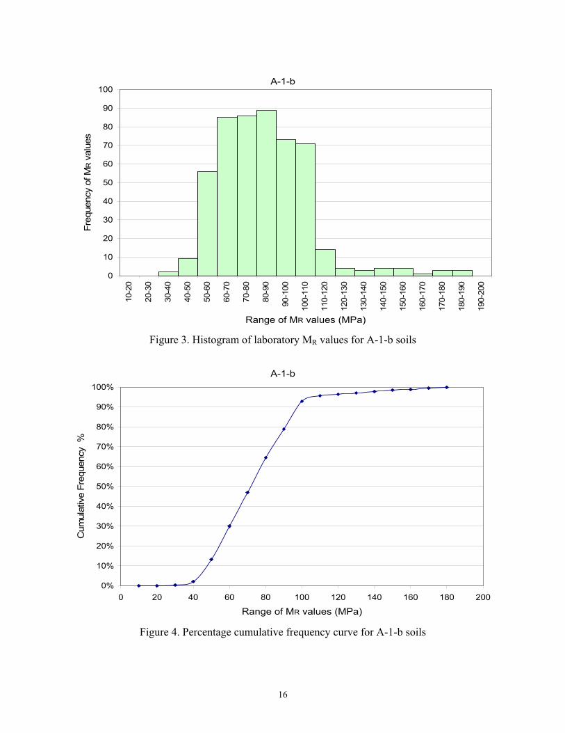
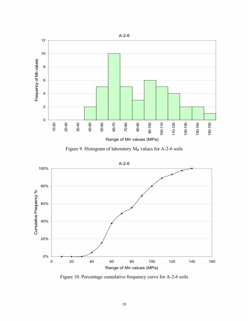
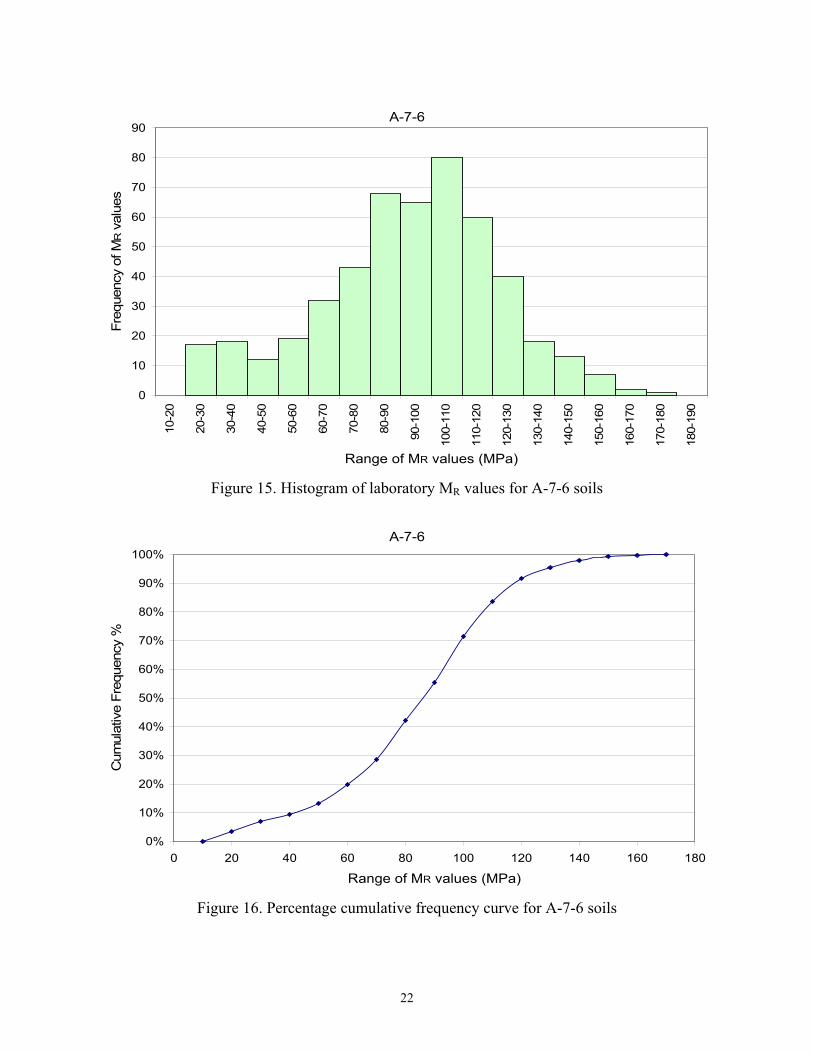
The data collected from LTPP database includes data for 8 AASHTO subgrade soil types namely, A-1-b, A-3, A-2-4, A-2-6, A-4, A-6, A-7-5, and A-7-6. Soils of class A-1-a, A-2-5, A-2-7, and A-5 were not found in the test sites considered here in this report. A list of LTPP test sites where laboratory resilient modulus (MR) and field FWD test data were available in the database are given in Appendix B (in accompanying CD.) All raw data extracted from LTPP database have been presented in Appendix I (in accompanying CD). Number of soil samples for which information is available in the LTPP database and collected for this study in each of the states considered (see list above) has been presented in Table 7. The soil samples include disturbed as well as undisturbed samples. Histograms and percentage cumulative frequency curves for the laboratory MR values for the 7 soil types A-1-b, A-3, A-2-4, A-2-6, A-4, A-6, and A-7-6 have been shown in Figure 3 through Figure 16. Soil type A-7-5 is not included in this study hereafter, since, test result of only one soil sample was available in the LTPP database for the regions considered.

15

Table 7. Total number of soil samples by states for which data collected from LTPP database AASHTO Soil Classification

State State Code A-1-a A-1-b A-3 A-2-4 A-2-5 A-2-6 A-2-7 A-4 A-5 A-6 A-7-5 A-7-6

New England Connecticut 9 - - - 3 - - - - - - - -

Maine 23 - 2 1 4 - - - - - - - - Massachusetts 25 - 1 1 - - - - - - - - -

New Hampshire 33 - - - - - - - - - - - -

Rhode Island 44 - - - - - - - - - - - - Vermont 50 - - - 3 - - - 2 - - - 1

Northern Mid Atlantic

New Jersey 34 - 4 1 3 - - - - - - - - New York 36 - 1 1 3 - - - 2 - - - -

Pennsylvania 42 - 2 - 8 - 1 - 11 - 3 - - Great Lakes

Illinois 17 - 1 1 1 - - - 11(2) - 2(1) - 1 Indiana 18 - 1 1 4 - - - 7(2) - 3(1) - 1

Michigan 26 - 2 8(1) 1 - - - 7 - 4 - - Minnesota 27 - 12 2 6 - 2(1) - 2 - 5(2) 1 1

Ohio 39 - - - - - - - 9 - 6 - 3 Wisconsin 55 - 3 4 - - - - 2 - 1 - -

Ontario 87 - - - - - - - 8 - 1 - - Quebec 89 - - 4 7 - - - - - - - -

Upper Mid West Iowa 19 - - - 4 - - - 5(3) - 11(6) - -

Kansas 20 - - 1 3 - - - 6(1) - 4(2) - 9(4) Missouri 29 - 2 - - - 3 - 6(1) - 4(1) - 6(1) Nebraska 31 - 2 - 2 - - - 8 - 4 - 7(3)

North Dakota 38 - - - - - - - 2 - - - - South Dakota 46 - 1 - - - - - 6(1) - 7(2) - 4

Total 0 34 25(1) 52 0 6 0 94(10) 0 55(15) 1 33(8)

* Numbers in parentheses are the number of undisturbed samples

16

A-1-b

0

10

20

30

40

50

60

70

80

90

100

10-2

0

20-3

0

30-4

0

40-5

0

50-6

0

60-7

0

70-8

0

80-9

0

90-1

00

100-

110

110-

120

120-

130

130-

140

140-

150

150-

160

160-

170

170-

180

180-

190

190-

200

Range of MR values (MPa)

Freq

uenc

y of

MR v

alue

s

Figure 3. Histogram of laboratory MR values for A-1-b soils

A-1-b

0%

10%

20%

30%

40%

50%

60%

70%

80%

90%

100%

0 20 40 60 80 100 120 140 160 180 200


Cum

ulat

ive

Freq

uenc

y %

Figure 4. Percentage cumulative frequency curve for A-1-b soils

17

A-3

0

10

20

30

40

50

60

70

80

10-2

0

20-3

0

30-4

0

40-5

0

50-6

0

60-7

0

70-8

0

80-9

0

90-1

00

100-

110

110-

120

120-

130

130-

140


Freq

uenc

y of

MR v

alue

s

Figure 5. Histogram of laboratory MR values for A-3 soils

A-3

0%

10%

20%

30%

40%

50%

60%

70%

80%

90%

100%

0 20 40 60 80 100 120 140


Cum

ulat

ive

Freq

uenc

y %

Figure 6. Percentage cumulative frequency curve for A-3 soils

18

A-2-4

0

20

40

60

80

100

120

140

160

180

10-2

0

20-3

0

30-4

0

40-5

0

50-6

0

60-7

0

70-8

0

80-9

0

90-1

00

100-

110

110-

120

120-

130

130-

140

140-

150

150-

160

160-

170


Freq

uenc

y of

MR v

alue

s

Figure 7. Histogram of laboratory MR values for A-2-4 soils

A-2-4

0%

10%

20%

30%

40%

50%

60%

70%

80%

90%

100%

0 20 40 60 80 100 120 140 160


Cum

ulat

ive

Freq

uenc

y %

Figure 8. Percentage cumulative frequency curve for A-2-4 soils

19

A-2-6

0

2

4

6

8

10

12

10-2

0

20-3

0

30-4

0

40-5

0

50-6

0

60-7

0

70-8

0

80-9

0

90-1

00

100-

110

110-

120

120-

130

130-

140

140-

150


Freq

uenc

y of

MR v

alue

s


A-2-6

0%

20%

40%

60%

80%

100%

0 20 40 60 80 100 120 140 160


Cum

ulat

ive

Freq

uenc

y %


20

A-4

0

20

40

60

80

100

120

140

160

180

200

10-2

0

20-3

0

30-4

0

40-5

0

50-6

0

60-7

0

70-8

0

80-9

0

90-1

00

100-

110

110-

120

120-

130

130-

140

140-

150

150-

160

160-

170

170-

180

180-

190

190-

200

200-

210

210-

220

220-

230

230-

240

240-

250

250-

260


Freq

uecn

y of

MR v

alue

s


A-4

0%

10%

20%

30%

40%

50%

60%

70%

80%

90%

100%

0 20 40 60 80 100 120 140 160 180 200 220 240 260


Cum

ulat

ive

Freq

uenc

y %


21

A-6

0

10

20

30

40

50

60

70

80

90

100

10-2

0

20-3

0

30-4

0

40-5

0

50-6

0

60-7

0

70-8

0

80-9

0

90-1

00

100-

110

110-

120

120-

130

130-

140

140-

150

150-

160

160-

170

170-

180

180-

190

190-

200

200-

210

210-

220

220-

230

230-

240

240-

250

250-

260


Freq

uenc

y of

MR v

alue

s


A-6

0%

10%

20%

30%

40%

50%

60%

70%

80%

90%

100%

0 20 40 60 80 100 120 140 160 180 200 220 240 260


Cum

ulat

ive

Freq

uenc

y %


22

A-7-6

0

10

20

30

40

50

60

70

80

90

10-2

0

20-3

0

30-4

0

40-5

0

50-6

0

60-7

0

70-8

0

80-9

0

90-1

00

100-

110

110-

120

120-

130

130-

140

140-

150

150-

160

160-

170

170-

180

180-

190


Freq

uenc

y of

MR v

alue

s


A-7-6

0%

10%

20%

30%

40%

50%

60%

70%

80%

90%

100%

0 20 40 60 80 100 120 140 160 180


Cum

ulat

ive

Freq

uenc

y %


23

4.2 Variation of Resilient Modulus (MR) with Stress Levels

During the laboratory resilient modulus test, the test specimen is subjected to 5 levels of cyclic stress (approximately 12.4, 24.8, 37.3, 49.7, and 62.0 kPa) at each of the 3 levels of confining pressure (13.8, 27.6, 41.4 kPa). Previous studies have shown that MR varies with the change in stresses. To investigate this effect, for the data extracted from LTPP database, resilient modulus values were plotted against the nominal maximum axial stress and confining pressure for certain number of representative soil samples in each of the 7 AASHTO subgrade soil types mentioned in earlier section. The results are given in Figures 17 through 32. It was observed that for the granular soils like A-1-b, A-3, and A-2-4, MR usually increased with increase in nominal maximum axial stress at the same level of confining pressure. However, for silty-clay soils like A-4, A-6, and A-7-6 there was a general trend of decrease in MR with increase in nominal maximum axial stress at the same level of confining pressure. Figures 17 through 32 show that generally, there is an increase in MR with the increase in confining pressure.

A-1-b

0

20

40

60

80

100

120

0 13.8 27.6 41.4 55.2 69 82.8Nominal Maximum Axial Stress (kPa)

Lab

M R

(MP

a)

23-7023-1-13.8 *

23-7023-2-13.8

25-1004-1-13.8

23-7023-1-27.6

23-7023-2-27.6

25-1004-1-27.6

23-7023-1-41.4

23-7023-2-41.4

25-1004-1-41.4

Figure 17. Nominal Maximum Axial Stress vs. MR for A-1-b soils in New England at 3 levels of Confining Pressure (* State Code-SHRP ID-Test No.-Confining Pressure in kPa)

24

A-3

0

20

40

60

80

100

0 13.8 27.6 41.4 55.2 69 82.8

Nominal Maximum Axial Stress (kPa)

Lab

M R

(MP

a) 23-3013-2-13.8 *

25-1002-2-13.8

23-3013-2-27.6

25-1002-2-27.6

23-3013-2-41.4

25-1002-2-41.4

Figure 18. Nominal Maximum Axial Stress vs. MR for A-3 soils in New England at 3 levels of Confining Pressure (* State Code-SHRP ID-Test No.-Confining Pressure in kPa)

A-2-4 (Confining Pressure=13.8 KPa)

0

20

40

60

80

100

120

0 13.8 27.6 41.4 55.2 69 82.8


Lab

M R

(MP

a)

9-4008-1 *

9-4008-2

9-4020-1

9-5001-1

23-0506-2

23-1012-1

23-1012-2

23-1026-1

23-3014-1

50-1681-1

50-1681-2

50-1682-2

Figure 19. Nominal Maximum Axial Stress vs. MR for A-2-4 soils in New England at Confining Pressure of 13.8 kPa (* State Code-SHRP ID-Test No.)

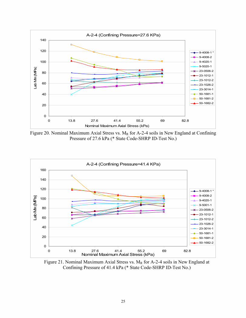
25


0

20

40

60

80

100

120

140

0 13.8 27.6 41.4 55.2 69 82.8


Lab

M R

(MPa

)

9-4008-1 *

9-4008-2

9-4020-1

9-5020-1

23-0506-2

23-1012-1

23-1012-2

23-1026-2

23-3014-1

50-1681-1

50-1681-2

50-1682-2

Figure 20. Nominal Maximum Axial Stress vs. MR for A-2-4 soils in New England at Confining Pressure of 27.6 kPa (* State Code-SHRP ID-Test No.)


0

20

40

60

80

100

120

140

160


Lab

M R

(MP

a)

9-4008-1 *

9-4008-2

9-4020-1

9-5001-1

23-0506-2

23-1012-1

23-1012-2

23-1026-2

23-3014-1

50-1681-1

50-1681-2

50-1682-2

Figure 21. Nominal Maximum Axial Stress vs. MR for A-2-4 soils in New England at

Confining Pressure of 41.4 kPa (* State Code-SHRP ID-Test No.)

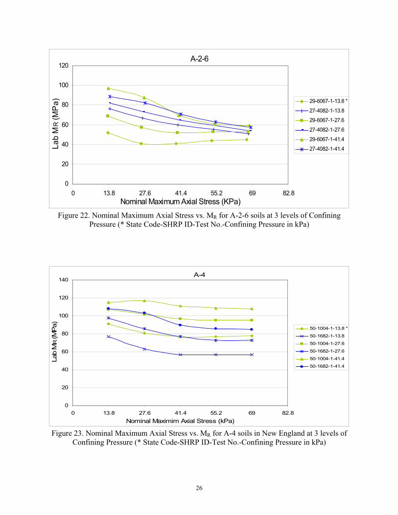
26

A-2-6

0

20

40

60

80

100

120

0 13.8 27.6 41.4 55.2 69 82.8Nominal Maximum Axial Stress (KPa)

Lab

M R

(MP

a) 29-6067-1-13.8 *

27-4082-1-13.8

29-6067-1-27.6

27-4082-1-27.6

29-6067-1-41.4

27-4082-1-41.4

Figure 22. Nominal Maximum Axial Stress vs. MR for A-2-6 soils at 3 levels of Confining Pressure (* State Code-SHRP ID-Test No.-Confining Pressure in kPa)

A-4

0

20

40

60

80

100

120

140

0 13.8 27.6 41.4 55.2 69 82.8Nominal Maximim Axial Stress (kPa)

Lab

M R

(MP

a) 50-1004-1-13.8 *

50-1682-1-13.8

50-1004-1-27.6

50-1682-1-27.6

50-1004-1-41.4

50-1682-1-41.4

Figure 23. Nominal Maximum Axial Stress vs. MR for A-4 soils in New England at 3 levels of Confining Pressure (* State Code-SHRP ID-Test No.-Confining Pressure in kPa)

27

A-6

0

20

40

60

80

100

120

140


Lab

M R

(MP

a) 42-1608-1-13.8 *

42-7037-1-13.8

42-1608-1-27.6

42-7037-1-27.6

42-1608-1-41.4

42-7037-1-41.4

Figure 24. Nominal Maximum Axial Stress vs. MR for A-6 soils at 3 levels of Confining Pressure (* State Code-SHRP ID-Test No.-Confining Pressure in kPa)

A-7-6

0

20

40

60

80

100

120


Lab

M R

(MP

a) 50-1004-2-13.8 *

20-0203-2-13.8

50-1004-2-27.6

20-0203-2-27.6

50-1004-2-41.4

20-0203-2-41.4

Figure 25. Nominal Maximum Axial Stress vs. MR for A-7-6 soils at 3 levels of Confining Pressure (* State Code-SHRP ID-Test No.-Confining Pressure in kPa)

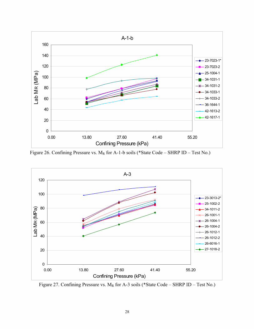
28

A-1-b

0

20

40

60

80

100

120

140

160

0.00 13.80 27.60 41.40 55.20Confining Pressure (kPa)

Lab

M R

(MP

a)

23-7023-1*

23-7023-2

25-1004-1

34-1031-1

34-1031-2

34-1033-1

34-1033-2

36-1644-1

42-1613-2

42-1617-1

Figure 26. Confining Pressure vs. MR for A-1-b soils (*State Code – SHRP ID – Test No.)

A-3

0

20

40

60

80

100

120


Lab

M R

(MP

a)

23-3013-2*

25-1002-2

34-1011-2

26-1001-1

26-1004-1

26-1004-2

26-1012-1

26-1012-2

26-6016-1

27-1018-2

Figure 27. Confining Pressure vs. MR for A-3 soils (*State Code – SHRP ID – Test No.)

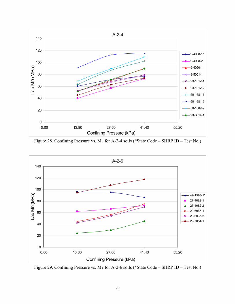
29

A-2-4

0

20

40

60

80

100

120

140


Lab

M R

(MP

a)

9-4008-1*

9-4008-2

9-4020-1

9-5001-1

23-1012-1

23-1012-2

50-1681-1

50-1681-2

50-1682-2

23-3014-1

Figure 28. Confining Pressure vs. MR for A-2-4 soils (*State Code – SHRP ID – Test No.)

A-2-6

0

20

40

60

80

100

120

140

0.00 13.80 27.60 41.40 55.20

Confining Pressure (kPa)

Lab

M R

(MP

a) 42-1598-1*

27-4082-1

27-4082-2

29-6067-1

29-6067-2

29-7054-1


30

A-4

0

20

40

60

80

100

120

0.00 13.80 27.60 41.40 55.20

Confining Pressure (KPa)

Lab

M R (M

Pa)

50-1004-1*

50-1682-1

36-1008-2

36-1011-1

42-1597-2

42-1599-1

42-1606-1

42-1617-2

42-1618-1

42-5020-1


A-6

0

20

40

60

80

100

120

140

160

180


Lab

M R

(MP

a)

42-1606-2*

42-1608-1

42-7037-1

17-5908-1

17-5908-2

18-4021-1

18-5043-2

27-6300-1

18-4021-2

27-6300-2


31

A-7-6

0

20

40

60

80

100

120


Lab

M R

(MP

a)

50-1004-2*

17-6050-1

18-5043-1

27-9075-2

39-9006-2

39-9022-1

39-9022-2

20-3013-1

20-3013-2

20-3015-1


4.3 Resilient Modulus Prediction Models

The determination of MR using the repeated load triaxial test is a very sophisticated process that requires substantial time and resources. Therefore, most of the State Highway agencies prefer not to measure MR in the laboratory frequently. Nondestructive deflection testing devices like the Falling Weight Deflectometer can also be used to measure the insitu modulus of the subgrade soil using backcalculation process. But from the studies so far, a definite relationship between the laboratory and backcalculated modulus value has not been established. Estimation of MR from physical properties has been studied by several investigators in the past because tests for determining the physical properties are much simpler and cheaper than the test for direct evaluation of MR itself. Moreover, the correlation of MR with the physical properties allows the study of the seasonal effect on the value of MR. Some of the studies that have developed prediction models for estimating the value of MR from a set of physical properties and applied stresses during repeated load test include Santha (1994), Von Quintus and Killingsworth (1998) Mohammad et al (1999), and Yau and Von Quintus (2002).

Prediction models for estimating MR values have been developed in this study for AASHTO

soil types A-1-b, A-3, A-2-4, A-4, A-6, and A-7-6. Prediction model for soil type A-2-6 could not be developed due to only small number of samples being available under this type. Only the reconstituted/disturbed test specimen test results have been used in developing these prediction models. Yau and Von Quintus (2002) have noted that sampling technique (disturbed/ undisturbed test specimens) of subgrade soils has an effect on the MR test results for all soil groups (gravel, silt, clay) except sand. Von Quintus and Killingsworth (1998) observed significant improvement in correlation between MR and soil physical properties when disturbed

32

and undisturbed samples were separated for model prediction. Hence in this study we have considered only the reconstituted specimens. Prediction models for undisturbed soil specimens have not been developed because very little data is available for each soil type.

Resilient modulus test results that have been identified as anomaly in the report “Study of

LTPP Laboratory Resilient Modulus Test Data and Response Characteristics” (Yau and Von Quintus 2002) have not been included in this study. Numbers of total, reconstituted/disturbed, and undisturbed soil samples available for the 6 AASHTO soil types (A-1-b, A-3, A-2-4, A-4, A-6, and A-7-6) are presented in Table 8. Disturbed/Reconstituted soil samples are those which have experienced structural disturbances during the sampling operation and are recompacted in the laboratory before MR test while undisturbed samples are those in which structural disturbance is kept to a minimum during the sampling process and are tested as obtained from the test site.

Three prediction models have been developed for each AASHTO soil type. The first set of models is the composite model that has been developed from all reconstituted soil specimens (MODEL1), the second set of models is from only those samples that have been compacted at the optimum moisture content only during MR testing (MODEL2) and the third model set of models have been developed from the samples that have been compacted at insitu moisture content (MODEL3). Total of 259 test specimens have been included: 34 samples for A-1-b soils, 24 samples for A-3 soils, 52 samples for A-2-4 soils, 84 samples for A-4 soils, 40 samples for A-6 samples and 25 samples of A-7-6 soils. Only the tests with Record Status “E” in the LTPP database have been entered in this study as only these tests have passed all levels of LTPP quality control checks (see Appendix I.4 for details on LTPP quality control checks) Table 8. Number of samples by AASHTO soil types for which data was extracted from the LTPP database Soil Type

Total samples

Disturbed/Reconstituted samples

Undisturbed Samples

A-1-b 34 34 - A-3 25 24 1 A-2-4 52 52 - A-4 94 84 10 A-6 55 40 15 A-7-6 33 25 8 Total 293 259 34

4.3.1 Generalized Constitutive Model

Several constitutive models have been developed in the past in order to describe the nonlinear behavior of MR for subgrade soils. Some of these models consisted of bulk stress only for granular soils or deviator stress only for cohesive soils or both bulk stress and deviator stress called universal model (Smart and Humphrey, 1999). The 2002 Design Guide suggests the use of the following generalized constitutive model for estimation of MR:

32

1

k

a

oct

k

aaR PP

PkM ⎟⎟⎠

⎞⎜⎜⎝

⎛⎟⎟⎠

⎞⎜⎜⎝

⎛=

τθ

………………………………………….. (2)

33

where, MR = Resilient modulus Pa = Normalizing stress (atmospheric pressure)

k1, k 2, k3 = Regression coefficients θ = Bulk stress = σ1 + σ2 + σ3 ………………. (3) σ1 = Major principal stress σ2 = Intermediate principal stress ( = σ3 for MR test on cylindrical specimen) σ3 = Minor principal stress / Confining pressure τoct = Octahedral shear stress

= 31 ( ) ( ) ( )2

322

312

21 σσσσσσ −+−+− …………….. (4)

According to the 2002 Design Guide either linear or nonlinear regression analysis may be

used to fit the analytical prediction model to laboratory generated MR test data. Coefficient k1 is directly proportional to Young’s modulus. Hence, it cannot have a negative value since MR cannot be negative. k2 should be positive since increasing the bulk stress should produce stiffening effect on the material which results in higher MR. Hence, the exponent of bulk stress (θ) should be positive. Similarly, k3 should be negative since increase of shear stress produces softening effect on the material which results in lower MR. Therefore, the exponent of octahedral shear stress (τoct), k3 should be negative. 4.3.2 Regression Analysis Methodology

Multiple linear regression technique was carried out to determine the value of coefficients k1, k2, and k3 for each individual soil specimen. Computer software SAS® 9.1 (2002-2003) was used for conducting the regression analysis. Equation (2) was transformed to the following form by taking logarithm on both sides to carry out linear regression:

( ) ⎟⎟⎠

⎞⎜⎜⎝

⎛+⎟⎟

⎠

⎞⎜⎜⎝

⎛+=

a

oct

aaR P

kP

kPkMτθ loglogloglog 321 …………………………….. (5)

Regression was carried out between laboratory measured MR values and the corresponding values of bulk stress and octahedral shear stress to get values of k1, k2, and k3 for each sample. In the LTPP testing each sample was tested at 5 levels of deviator stress (12.4, 24.8, 37.3, 49.7 and 62.0 kPa) for 3 levels of confining pressure (13.8, 27.6 and 41.4 kPa) resulting in 15 combinations of stresses for each sample. Example of laboratory resilient modulus test results for one A-2-4 soil sample in Connecticut has been presented in Table 9. The complete set of MR test data for all samples considered in the current study can be found in Tables I.2.1 to I.2.4 in Appendix I available in accompanying CD. Here the cyclic stress applied during MR test has been taken equal to the deviator stress (σd) as suggested by various researchers in the past (Smart and Humphrey 1999). Deviator stress is given by,

σd = σ1 – σ3 ……………………….. (6) Here since, σ2 = σ3 and σd = σ1 – σ3, Eq. (4) reduces to

3

2 doct

στ

×= ……………………. (7)

34

Table 9. Sample Laboratory MR test data (one A-2-4 soil specimen from Connecticut) SHRP

ID

State Code

La- yer No.

Test No.

Loc_ No

Sample No.

Conf-ining Pres- sure kPa

Nom_ Max_ Axial_ Stress kPa

MR_ Matl_ Type

Appl. Cyclic Load Avg.

N

Appl. Cyclic Stress Avg. kPa

Appl. Contact Stress Avg. kPa

Resilient Strain Average

Resilient Modulus Average MPa

4008 9 1 2 BA* BS** 13.8 13.8 2 51.3 12.9 1.4 0.000349 37 4008 9 1 2 BA* BS** 13.8 27.6 2 102 25.8 2.8 0.000667 39 4008 9 1 2 BA* BS** 13.8 41.4 2 152 38.4 4.1 0.000929 41 4008 9 1 2 BA* BS** 13.8 55.2 2 200 50.5 5.5 0.001192 42 4008 9 1 2 BA* BS** 13.8 68.9 2 247 62.2 6.9 0.001535 41 4008 9 1 2 BA* BS** 27.6 13.8 2 51.9 13 1.4 0.000244 54 4008 9 1 2 BA* BS** 27.6 27.6 2 102 25.8 2.8 0.000479 54 4008 9 1 2 BA* BS** 27.6 41.4 2 153 38.5 4.1 0.000686 56 4008 9 1 2 BA* BS** 27.6 55.2 2 202 51 5.5 0.000866 59 4008 9 1 2 BA* BS** 27.6 68.9 2 251 63.4 6.9 0.001034 61 4008 9 1 2 BA* BS** 41.4 13.8 2 51.5 13 1.4 0.000195 66 4008 9 1 2 BA* BS** 41.4 27.6 2 102 25.7 2.8 0.000351 73 4008 9 1 2 BA* BS** 41.4 41.4 2 152 38.3 4.1 0.000518 74 4008 9 1 2 BA* BS** 41.4 55.2 2 201 50.8 5.5 0.000676 75 4008 9 1 2 BA* BS** 41.4 68.9 2 252 63.5 6.9 0.000829 77

The values of various stresses and MR used in Eq. (5) for each of the 15 combinations of

stresses for each soil sample in the first step regression analysis are presented in Tables C.1 to C.6 in Appendix C. Since the applied cyclic stress or deviator stress (σd) and the confining pressure (σ3) are known (measured), the major principal stress (σ1) is computed from Eqn. (6). Thereafter, the bulk stress (θ) is computed using Eq. (3). The octahedral shear stress (τoct) is computed using Eq. (7). For an example, stresses (θ, and τoct) and MR values used in the first step regression for one A-2-4 soil sample in Connecticut has been presented in Table 10.

Table 10. Sample stress and MR values used in First Step Regression State Code

SHRP ID

TN Confining Pressure, σ3 (kPa)

Deviator (Applied Cyclic)Stress, σd = σ1 -

σ3 (kPa)

Resilient Modulus,

MR (MPa)

Bulk Stress, θ=σ1+σ2+ σ3

(kPa)

Octahedral Stress, τoct

(kPa) log(MR) log(θ1/

Pa) log(τoct/

Pa) 9 4008 2 13.8 12.9 37 54.3 6.081 1.568 -0.271 -1.222 9 4008 2 13.8 25.8 39 67.2 12.162 1.591 -0.178 -0.921 9 4008 2 13.8 38.4 41 79.8 18.102 1.613 -0.103 -0.747 9 4008 2 13.8 50.5 42 91.9 23.806 1.623 -0.042 -0.629 9 4008 2 13.8 62.2 41 103.6 29.321 1.613 0.009 -0.539 9 4008 2 27.6 13 54 95.8 6.128 1.732 -0.025 -1.222 9 4008 2 27.6 25.8 54 108.6 12.162 1.732 0.03 -0.921 9 4008 2 27.6 38.5 56 121.3 18.149 1.748 0.078 -0.747 9 4008 2 27.6 51 59 133.8 24.041 1.771 0.121 -0.625 9 4008 2 27.6 63.4 61 146.2 29.887 1.785 0.159 -0.53 9 4008 2 41.4 13 66 137.2 6.128 1.82 0.132 -1.222 9 4008 2 41.4 25.7 73 149.9 12.115 1.863 0.17 -0.921 9 4008 2 41.4 38.3 74 162.5 18.055 1.869 0.205 -0.75 9 4008 2 41.4 50.8 75 175 23.947 1.875 0.237 -0.627 9 4008 2 41.4 63.5 77 187.7 29.934 1.886 0.268 -0.53

35

It must be noted here that since the applied cyclic/deviator stress (σd) during the tests is nearly the same from one sample to another and so is σ3 , the values of σ1, θ, and τoct calculated are more or less the same for all the samples.

In this study, the unit used for MR is MPa and for values of stresses (θ, τoct, and Pa) appearing

on the right side of Eq. (2) is kPa. The value of atmospheric pressure (Pa) used in this study is 101.325 kPa which is the standard atmospheric pressure at sea level. List of k values and the corresponding R2 values obtained after regression for each sample has been reported in Tables D.1 to D.6, Appendix D for soil types A-1-b, A-3, A-2-4, A-4, A-6, and A-7-6 respectively.

After obtaining k1, k2, and k3 for each soil sample, a second set of regression was carried out

to relate these k values with the physical properties of soil for the 6 types of subgrade soils, AASHTO A-1-b, A-3, A-2-4, A-4, A-6, and A-7-6. The soil properties that were considered for the study are:

Specimen moisture content (MC) Optimum moisture content (OMC) Moisture content ratio (MCR=MC/OMC) Specimen dry density (DD) Maximum dry density (MAXDD) Dry density ratio (DDR=DD/MAXDD) Liquid limit (LL) Plastic limit (PL) Percent passing 3” sieve (S3) Percent passing 2” sieve (S2) Percent passing 1 1/2” sieve (S1_HALF) Percent passing 1” sieve (S1) Percent passing 3/4” sieve (S3_4) Percent passing 1/2” sieve (S1_2) Percent passing 3/8” sieve (S3_8) Percent passing #4 sieve (SN4) Percent passing #10 sieve (SN10) Percent passing #40 sieve (SN40) Percent passing #80 sieve (SN80) Percent passing #200 sieve (SN200) Percent coarse sand (CSAND, particles of size 2 – 0.42 mm) Percent fine sand (FSAND, particles of size 0.42 - .074 mm) Percent silt (SILT, particles of size 0.074 – 0.002 mm) Percent clay (CLAY, particles of size 0.002 mm). Soil samples that gave negative values for k1 and k2, or positive values for k3 were not used

in the second set regression for the reasons noted above in Section “Generalized Constitutive Model.” The 2002 Design Guide suggests using the k-values from those individual samples that yield multiple correlation coefficient (R2) equal to 0.9 or higher from the regression analysis of MR using Eq. (5). Otherwise, consideration should be given to use different constitutive model for soil samples yielding R2 less than 0.90. Therefore, in this study only the samples that resulted in R2 equal to 0.90 or above from the regression analysis of MR relation (Eq. ( 5)) were included in the overall regression for a particular soil type to develop models relating coefficients, k1, k2, and k3, with the soil properties. The properties of each soil sample that were used in second step regression for each AASHTO soil type has been presented in Tables D.7 to D.12 in Appendix D.

The mean and range of k-coefficient (k1, k2, and k3) values obtained for the individual soil

specimens from the regression analysis of Eq. (5) that were used in the second set regression analysis of all reconstituted samples for the 6 different AASHTO soil types have been presented in Table 11 below. Similar data for the models containing only those samples compacted at optimum moisture content or only the samples compacted at insitu moisture content only have

36

been presented in Tables 12 and 13. The values of k coefficients obtained for individual soil sample have been presented in Tables D.1 to D.6 in Appendix D.

Table 11. Range of k coefficients for all reconstituted samples used in second step regression AASHTO Soil Type

Variable No. of Samples

Mean Standard Deviation

Minimum Maximum

k1 29 0.5077 0.1243 0.2817 1.0142k2 29 0.6863 0.0985 0.4689 0.8493A-1-b k3 29 -0.1426 0.0703 -0.3579 -0.0089k1 19 0.5019 0.0575 0.3697 0.5834k2 19 0.6675 0.0676 0.5681 0.8219A-3 k3 19 -0.1097 0.0252 -0.1493 -0.0545k1 40 0.4198 0.0895 0.2163 0.6685k2 40 0.6295 0.1426 0.2857 0.8830

A-2-4

k3 40 -0.2005 0.0853 -0.4150 -0.0845k1 66 0.4398 0.2295 0.1293 1.2192k2 66 0.4462 0.1579 0.1696 0.9885A-4

k3 66 -0.2871 0.1033 -0.5701 -0.0902k1 36 0.5116 0.3569 0.1202 1.5382k2 36 0.3016 0.1280 0.1742 0.8854A-6 k3 36 -0.3028 0.1535 -0.6281 -0.0390k1 20 0.5244 0.2735 0.0664 1.0578k2 20 0.2309 0.0793 0.1305 0.4707

A-7-6

k3 20 -0.2399 0.1551 -0.6198 -0.0924

Table 12. Range of k coefficients for samples compacted at optimum moisture content used in second step regression AASHTO Soil Type



Minimum Maximum

k1 10 0.5136 0.0781 0.4361 0.6830k2 10 0.7113 0.0721 0.5991 0.8145A-1-b k3 10 -0.1222 0.0671 -0.2541 -0.0089k1 14 0.5029 0.0559 0.3697 0.5834k2 14 0.6600 0.0611 0.5681 0.7498A-3 k3 14 -0.1104 0.0285 -0.1493 -0.0545k1 28 0.4329 0.0899 0.2163 0.6685k2 28 0.6217 0.1431 0.2857 0.8830

A-2-4

k3 28 -0.2019 0.0916 0.4150 -0.0845k1 41 0.4896 0.2349 0.1663 1.2192k2 41 0.4115 0.1233 0.1696 0.6666A-4

k3 41 -0.2882 0.1011 -0.5701 -0.1043k1 23 0.5194 0.3171 0.1202 1.2086k2 23 0.2896 0.0796 0.1844 0.5693A-6 k3 23 -0.3057 0.1694 -0.6281 -0.0390k1 13 0.5935 0.1964 0.2491 0.9793k2 13 0.2181 0.0584 0.1488 0.3660

A-7-6

k3 13 -0.1920 0.0759 -0.3428 -0.0946

37

Table 13. Range of k coefficients for samples compacted at insitu moisture content used in second step regression AASHTO Soil Type



Minimum Maximum

k1 19 0.5046 0.1448 0.2817 1.0142 k2 19 0.6732 0.1094 0.4689 0.8493 A-1-b k3 19 -0.1534 0.0712 -0.3579 -0.0696 k1 4 0.4844 0.0702 0.3965 0.5639 k2 4 0.7083 0.0872 0.6259 0.8218 A-3 k3 4 -0.1065 0.0168 -0.1180 -0.0821 k1 12 0.3892 0.0843 0.2531 0.5044 k2 12 0.6478 0.1461 0.3306 0.8759

A-2-4

k3 12 -0.1972 0.0718 -0.3278 -0.0904 k1 25 0.3582 0.1989 0.1293 0.9789 k2 25 0.5031 0.1916 0.2552 0.9885 A-4

k3 25 -0.2853 0.1089 -0.5348 -0.0902 k1 13 0.4978 0.4323 0.1428 1.5382 k2 13 0.3228 0.1881 0.1742 0.8854 A-6 k3 13 -0.2977 0.1270 -0.4939 -0.0941 k1 8 0.4823 0.4135 0.0664 1.0849 k2 8 0.2602 0.1027 0.1305 0.4707

A-7-6

k3 8 -0.3007 0.2227 -0.6198 -0.0924 In the second set of regression analysis, a list of models was first printed using RSQUARE

selection method available in SAS® (2002-2003). The RSQUARE method gives several subsets of independent variables that best predict a dependent variable by linear regression in the given sample (SAS® 9.1.3, 2002-2003). A sample partial output of RSQUARE selection method for the k3 coefficient of A-2-4 soil (all reconstituted samples included) has been presented in Table 14. From this set of models, a model which had higher value of R2, with the Variance Inflation Factor (VIF) for the variables less than 10 was selected. As a rule of thumb, variables with VIF greater than 10 are to be investigated to check for multicollinearity (Chen et al 2004). Chatterjee and Price (1977) have mentioned that VIF in excess of 10 is an indication that multicollinearity may cause problems in estimation. Besides R2, adjusted (adj.) R2 value was also examined while selecting a model. Ordinary R2 value always increases (at least not decrease) as more number of predictor variables are added to the model even if the variables are not related significantly to the variable to be predicted (Montgomery and Peck 1992). But the adjusted R2 can decrease if unnecessary terms are added. The adjusted R2 value gives a more honest estimation of R2 (Chen et al 2004) and guards against addition of unnecessary terms. Therefore, a model which had higher adjusted R2 besides having high R2 was selected. Furthermore, while choosing the final model, a model that contains several relevant soil property predictors like moisture content, density, and gradation were preferred over a model having all gradation variables although it had higher R2. All the regression equations developed were checked to see if they satisfied the assumptions of linear regression like normality of residuals, homogeneity of variance. A sample partial output of the result of second step regression analysis for the k3 coefficient of A-2-4 soil (all reconstituted samples included) has been presented in Table 15.

38

Table 14. Partial output of RSQUARE selection method for the k3 coefficient of A-2-4 soil (all reconstituted samples) Number R-Square Variables in Model in Model 6 0.6804 OMC LL S2 SN10 FSAND CLAY 6 0.6771 MC DDR LL S2 SN10 CLAY 6 0.6767 OMC LL S2 SN4 FSAND CLAY 6 0.6766 OMC LL S1_HALF SN10 FSAND CLAY 6 0.6765 OMC LL S3_4 SN4 FSAND CLAY 6 0.6756 OMC LL S3_4 SN10 FSAND CLAY 6 0.6746 OMC LL S2 SN10 SN40 SILT 7 0.7146 OMC DD MaxDD DDR LL S2 FSAND 7 0.7146 OMC DD MaxDD DDR LL S3 FSAND 7 0.7115 OMC DD MaxDD DDR LL S1_HALF FSAND 7 0.7095 OMC DD MaxDD DDR LL S2 SN10 7 0.7087 OMC DD MaxDD DDR LL S3 SN10 7 0.7083 OMC DD MaxDD DDR LL S2 S1_2 7 0.7077 OMC DD MaxDD DDR LL S2 SN4 7 0.7066 OMC DD MaxDD DDR LL S2 S3_8 7 0.7063 OMC DD MaxDD DDR LL S3 SN4 7 0.7059 OMC DD MaxDD DDR LL S1_HALF SN10 7 0.7048 OMC DD MaxDD DDR LL S1 FSAND 7 0.7047 OMC DD MaxDD DDR LL S1_HALF SN4 7 0.7040 OMC DD MaxDD DDR LL S1_HALF S1_2 7 0.7033 OMC DD MaxDD DDR LL S1_HALF S3_8 7 0.7029 OMC DD MaxDD DDR LL S3_4 S1_2 7 0.7022 OMC DD MaxDD DDR LL S3 S3_8 7 0.7011 OMC DD MaxDD DDR LL S3 S1_2 7 0.7004 OMC DD MaxDD DDR LL S2 S3_4 7 0.7002 OMC DD MaxDD DDR LL S3 SN40 7 0.6996 OMC DD MaxDD DDR LL S2 SN40 7 0.6993 OMC DD MaxDD DDR PL S3 FSAND 7 0.6992 OMC DD MaxDD DDR LL S1 SN10 7 0.6988 OMC DD MaxDD DDR LL S1 SN4 7 0.6983 MC OMC DD MaxDD DDR LL FSAND 7 0.6982 OMC MCR DD MaxDD DDR LL FSAND 7 0.6979 OMC DD MaxDD DDR LL S3_4 SN4 7 0.6978 OMC DD MaxDD DDR LL S3_4 S3_8 7 0.6978 OMC DD MaxDD DDR LL S3_4 FSAND 7 0.6973 OMC DD MaxDD DDR LL S1 S1_2 7 0.6969 OMC DD MaxDD DDR LL S3_4 SN10 7 0.6958 OMC DD MaxDD DDR LL S1 S3_8 7 0.6939 OMC DD MaxDD DDR LL S1_HALF SN40 7 0.6935 OMC MCR DD MaxDD DDR LL SN40 7 0.6933 OMC MCR LL S2 SN40 SN80 CLAY --->>> SELECTED MODEL 7 0.6931 MC OMC LL S2 SN10 FSAND CLAY 7 0.6929 OMC DD MaxDD DDR PL S3 S3_8

8 0.7370 MC OMC DD MaxDD DDR LL S3 SN10 8 0.7362 MC MCR DD MaxDD DDR LL S2 SN10 8 0.7361 MC OMC DD MaxDD DDR LL S2 SN10 8 0.7359 MC OMC DD MaxDD DDR LL S2 S1_2 8 0.7359 MC MCR DD MaxDD DDR LL S3 SN10 8 0.7354 MC OMC DD MaxDD DDR LL S3 SN4 8 0.7350 MC MCR DD MaxDD DDR LL S2 SN4

39

Table 15. Partial output of regression for the model selected for the k3 coefficient of A-2-4 soil (all reconstituted samples)

The REG Procedure

Model: MODEL1 Dependent Variable: K3 K3 Number of Observations Read 40 Number of Observations Used 40 Analysis of Variance Sum of Mean Source DF Squares Square F Value Pr > F Model 7 0.19669 0.02810 10.33 <.0001 Error 32 0.08700 0.00272 Corrected Total 39 0.28369 Root MSE 0.05214 R-Square 0.6933 Dependent Mean -0.20048 Adj R-Sq 0.6262 Coeff Var -26.00960 Parameter Estimates Parameter Standard Variance Variable Label DF Estimate Error t Value Pr > |t| Inflation Intercept Intercept 1 0.50825 0.21808 2.33 0.0262 0 OMC OMC 1 -0.01956 0.00668 -2.93 0.0063 1.66150 MCR MCR 1 -0.07234 0.05043 -1.43 0.1611 1.37691 LL LL 1 -0.00492 0.00112 -4.39 0.0001 1.78767 S2 S2 1 -0.00652 0.00238 -2.74 0.0101 1.40659 SN40 SN40 1 0.00384 0.00082932 4.63 <.0001 2.55033 SN80 SN80 1 -0.00153 0.00084707 -1.80 0.0807 1.54006 CLAY CLAY 1 0.00344 0.00235 1.47 0.1525 1.98084

4.3.3 Results of Regression Analysis 4.3.3.1 Soil Type: A-1-b

Thirty four test specimens from total of 13 states in the New England and nearby regions were initially analyzed to obtain the k coefficients (k1, k2, and k3) for individual soil samples with the known laboratory MR values using Eq. (5). Among these, 3 samples resulted in positive k3 and 2 samples resulted in R2 less than 0.90. These 5 samples were therefore not used for building the prediction models for k coefficients in the second step regression analysis that relates the k coefficients with the physical soil properties. Among the 29 samples that qualified for second step regression, 10 samples had been compacted at optimum moisture content and 19 samples had been compacted at insitu moisture content.

40

• All reconstituted samples: The final regression equations for k1, k2, and k3 obtained from the second step regression

analysis for all 29 reconstituted samples are as given below.

log k1 = 0.09931 - 0.00743 x MC + 0.00009293 x DD + 0.00505 x LL - 0.00466 x S3_8 - 0.01157 x SN200 (R2 = 0.57; Adj. R2 =0.47) (8)

k2 = -0.86401 - 0.01884 x OMC - 0.00116 x DD + 2.01898 x DDR + 0.02548 x S1 - 0.00691 x SN10 - 0.01047 x SN80 + 0.03127 x SILT (R2 = 0.68; Adj. R2 = 0.58) (9)

k3 = -0.74756 - 0.00913 x MC - 0.00041464 x DD - 0.00472 x PL + 0.03540 x S3 - 0.02075 x S2 (R2 = 0.55; Adj. R2 = 0.46) (10)

Plot for k coefficients obtained from first step regression against the predicted k coefficients determined from Eqs. (8), (9), and (10) along with 95% confidence interval lines has been presented in Figures 33, 34, and 35. Numerical values of these predicted k coefficients can be found in Table D.13, Appendix D.

The predicted values of MR can now be obtained by substituting available soil physical

properties values in the right hand side of Eqs. (8), (9), and (10) to determine k1, k2, and k3 respectively, and then using these predicted values of k coefficients into Eq. (5). The tabulated values of laboratory and predicted MR values has been presented in Tables C.1, Appendix C. The plot for predicted MR versus laboratory MR has been shown in Figure 36. The analysis of laboratory and predicted MR showed that 59.95 % of predicted MR values were within ± 10% of the laboratory MR values and 94.21 % of predicted MR values were within ± 20% of the laboratory MR values.

-0.7

-0.5

-0.3

-0.1

0.1

-0.7 -0.5 -0.3 -0.1 0.1Predicted log k1

log

k 1

Figure 33. log k1 vs. Predicted log k1 with 95% confidence interval line for all reconstituted soils for A-1-b soils

41

0.2

0.4

0.6

0.8

1

0.2 0.4 0.6 0.8 1 Predicted k2

k 2

Figure 34. k2 vs. Predicted k2 with 95% confidence interval line for all reconstituted soils for A-1-b soils

-0.5

-0.3

-0.1

0.1

-0.5 -0.3 -0.1 0.1Predicted k3

k 3

Figure 35. k3 vs. Predicted k3 with 95% confidence interval line for all reconstituted soils for A-1-b soils

42

0

50

100

150

200

0 50 100 150 200Laboratory MR (MPa)

Pred

icte

d M

R (M

Pa)

Figure 36. Predicted MR vs. Laboratory MR for all reconstituted samples for A-1-b soils

• Samples compacted at optimum moisture content :

Regression equations developed for the 10 A-1-b samples compacted at optimum moisture content are as follows: log k1 = -9.85454 - 0.01714 x OMC - 0.00078852 x DD + 0.11588 x S1_HALF - 0.00616 x SN10 +

0.00279 x FSAND (R2 = 0.99; Adj. R2 = 0.97) (11) k2 = -1.15403 + 0.03198 x OMC + 5.69990 x DDR - 0.04336 x S1_HALF + 0.01404 x SN40 +

0.00476 x CSAND - 0.00649 x FSAND (R2 = 0.99; Adj. R2 = 0.98) (12) k3 = 0.22460 - 0.02071 x OMC - 0.00010179 x MAXDD - 0.00046354 x SN10 - 0.00682 x SN40 +

0.00936 x FSAND (R2 = 0.99; Adj. R2 = 0.99) (13)

The plot of predicted MR calculated from the predicted values of k1, k2, and k3 from Eqs. (11), (12), and (13) against laboratory measured MR values has been presented in Figure 37 below. Numerical values of the predicted k coefficients can be found in Table D.13, Appendix D and numerical values for laboratory and predicted MR can be found in Table C.1, Appendix C. The analysis of laboratory and predicted MR showed that 96.00 % of predicted MR values were within ± 10% of the laboratory MR values and 98.00 % of predicted MR values were within ± 20% of the laboratory MR values.

43

0

50

100

150

200


Pre

dict

ed M

R (M

Pa)

Figure 37. Predicted MR vs. Laboratory MR for samples compacted at optimum moisture

content for A-1-b soils

• Samples compacted at in-situ moisture content: Results of second step regression for the 19 A-1-b soil samples compacted at insitu moisture

content have been presented in equations (14), (15), and (16) below.

log k1 = 1.78349 - 0.03097x MC + 0.00772 x LL - 0.01837 x S1_HALF - 0.01154 x SN200 (R2 = 0.71; Adj. R2 = 0.63) (14)

k2 = - 3.99018 - 0.06842 x MC + 0.49482 x MCR - 0.00185 x DD + 2.83862 x DDR + 0.06019 x S2 - 0.00774 x SN10 + 0.02423 x SILT (R2 = 0.80; Adj. R2 = 0.67) (15)

k3 = - 1.17525 - 0.01956 x MC - 0.00702 x PL + 0.02351 x S3 - 0.01190 x S1_HALF

(R2 = 0.60; Adj. R2 = 0.49) (16)

MR values predicted by substituting the predicted values of k coefficients given by equations (14), (15), and (16) in Eq. (5) were plotted against the laboratory measured MR values. The plot has been shown in Figure 38. Numerical values of the predicted k coefficients can be found in Table D.13, Appendix D and numerical values for laboratory and predicted MR can be found in Table C.1, Appendix C. The analysis of laboratory and predicted MR showed that 73.05 % of predicted MR values were within ± 10% of the laboratory MR values and 98.94 % of predicted MR values were within ± 20% of the laboratory MR values.

44

0

50

100

150

200


Pred

icte

d M

R (M

Pa)

Figure 38. Predicted MR vs. Laboratory MR for samples compacted at insitu moisture content for

A-1-b soils

4.3.3.2. Soil Type: A-3 In the first step regression analysis, 24 reconstituted samples from 11 states were analyzed

for A-3 soils. Five samples resulted in R2 less than 0.9 so only 19 samples were available for the second step regression. Among the 19 samples, 14 samples had been compacted at the optimum moisture content and 4 samples had been compacted at insitu moisture content. The results of second step regression for the 3 cases – All reconstituted samples, samples compacted at optimum moisture, and samples compacted at insitu moisture content have been presented below.

• All reconstituted samples:

The regression equations developed for the k coefficients for all reconstituted samples for A-3 soils are as given in Eq. (17), (18), and (19) below.

log k1 = - 0.93681 - 0.01248 x MC + 0.30352 x MCR + 0.00020285 x DD + 0.00194 x FSAND (R2 = 0.47; Adj. R2 = 0.32) (17)

k2 = - 0.13234 - 0.01724 x MC + 0.02560 x OMC + 0.00032543 x DD + 0.00313 x SN40 - 0.00291x

SN80 - 0.01843 x CLAY (R2 = 0.58; Adj. R2 = 0.38) (18)

k3 = - 1.03002 + 0.09865 x MCR + 0.00032615 x DD + 0.00220 x S1_HALF + 0.00067403 x SN40 (R2 = 0.76; Adj. R2 = 0.69) (19)

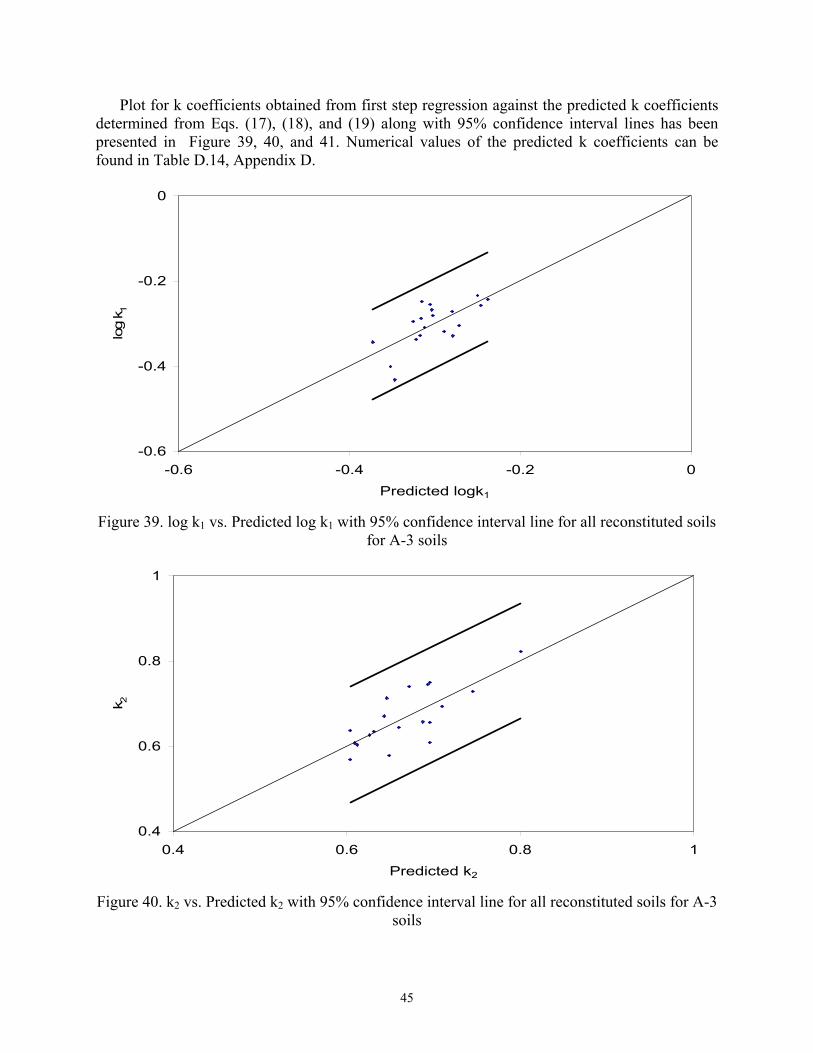
45

Plot for k coefficients obtained from first step regression against the predicted k coefficients determined from Eqs. (17), (18), and (19) along with 95% confidence interval lines has been presented in Figure 39, 40, and 41. Numerical values of the predicted k coefficients can be found in Table D.14, Appendix D.

-0.6

-0.4

-0.2

0

-0.6 -0.4 -0.2 0Predicted logk1

log

k 1

Figure 39. log k1 vs. Predicted log k1 with 95% confidence interval line for all reconstituted soils for A-3 soils

0.4

0.6

0.8

1

0.4 0.6 0.8 1Predicted k2

k 2

Figure 40. k2 vs. Predicted k2 with 95% confidence interval line for all reconstituted soils for A-3 soils

46

-0.2

-0.1

0

-0.2 -0.1 0Predicted k3

k 3


Plot for MR predicted by Eqs. (17), (18), and (19) and laboratory MR has been show in Figure

42. Tabulated values of laboratory and predicted MR values can be found in Table C.2, Appendix C. The analysis of laboratory and predicted MR showed that 63.73 % of predicted MR values were within ± 10% of the laboratory l MR values and 94.72 % of predicted MR values were within ± 20% of the laboratory MR values.

0

50

100

150

200


Pre

dict

ed M

R (M

Pa)

Figure 42. Predicted MR vs. Laboratory MR for all reconstituted samples for A-3 soils

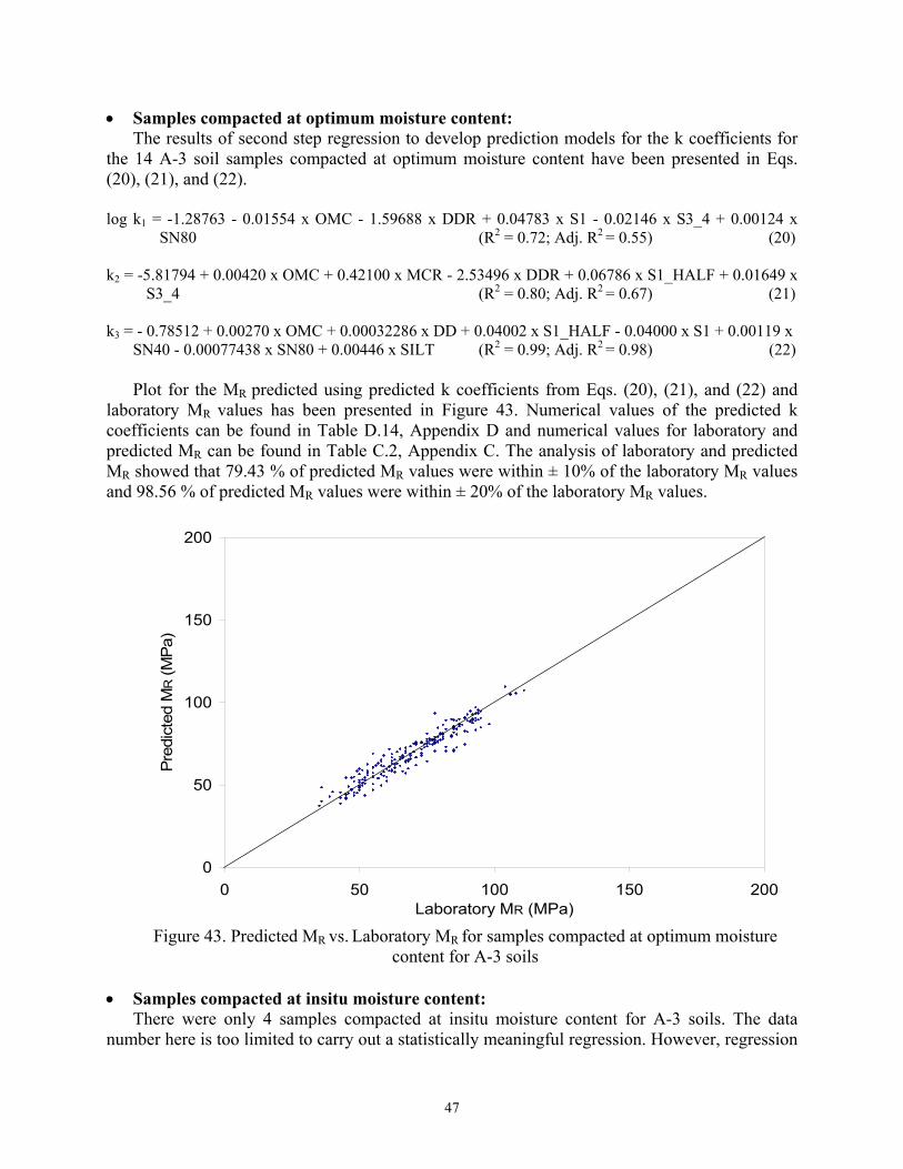
47

• Samples compacted at optimum moisture content: The results of second step regression to develop prediction models for the k coefficients for

the 14 A-3 soil samples compacted at optimum moisture content have been presented in Eqs. (20), (21), and (22).

log k1 = -1.28763 - 0.01554 x OMC - 1.59688 x DDR + 0.04783 x S1 - 0.02146 x S3_4 + 0.00124 x

SN80 (R2 = 0.72; Adj. R2 = 0.55) (20)

k2 = -5.81794 + 0.00420 x OMC + 0.42100 x MCR - 2.53496 x DDR + 0.06786 x S1_HALF + 0.01649 x S3_4 (R2 = 0.80; Adj. R2 = 0.67) (21)

k3 = - 0.78512 + 0.00270 x OMC + 0.00032286 x DD + 0.04002 x S1_HALF - 0.04000 x S1 + 0.00119 x

SN40 - 0.00077438 x SN80 + 0.00446 x SILT (R2 = 0.99; Adj. R2 = 0.98) (22)

Plot for the MR predicted using predicted k coefficients from Eqs. (20), (21), and (22) and laboratory MR values has been presented in Figure 43. Numerical values of the predicted k coefficients can be found in Table D.14, Appendix D and numerical values for laboratory and predicted MR can be found in Table C.2, Appendix C. The analysis of laboratory and predicted MR showed that 79.43 % of predicted MR values were within ± 10% of the laboratory MR values and 98.56 % of predicted MR values were within ± 20% of the laboratory MR values.

0

50

100

150

200


Pre

dict

ed M

R (M

Pa)


content for A-3 soils

• Samples compacted at insitu moisture content: There were only 4 samples compacted at insitu moisture content for A-3 soils. The data

number here is too limited to carry out a statistically meaningful regression. However, regression

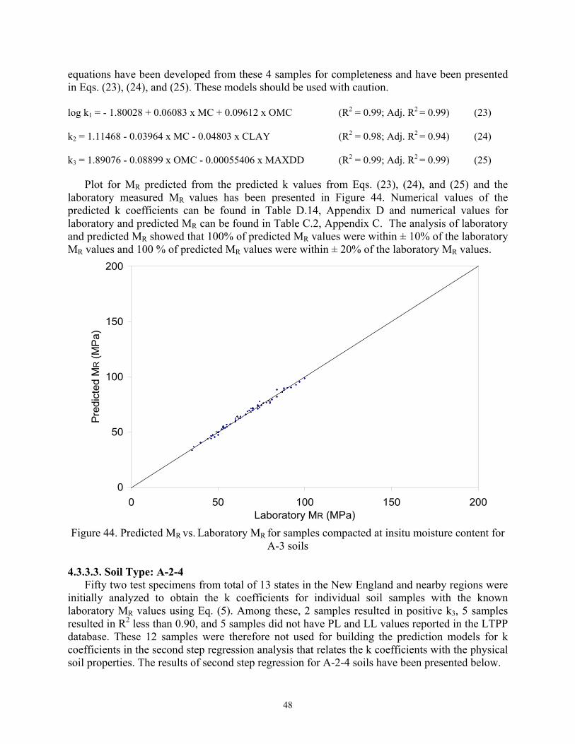
48

equations have been developed from these 4 samples for completeness and have been presented in Eqs. (23), (24), and (25). These models should be used with caution.

log k1 = - 1.80028 + 0.06083 x MC + 0.09612 x OMC (R2 = 0.99; Adj. R2 = 0.99) (23)

k2 = 1.11468 - 0.03964 x MC - 0.04803 x CLAY (R2 = 0.98; Adj. R2 = 0.94) (24)

k3 = 1.89076 - 0.08899 x OMC - 0.00055406 x MAXDD (R2 = 0.99; Adj. R2 = 0.99) (25)

Plot for MR predicted from the predicted k values from Eqs. (23), (24), and (25) and the

laboratory measured MR values has been presented in Figure 44. Numerical values of the predicted k coefficients can be found in Table D.14, Appendix D and numerical values for laboratory and predicted MR can be found in Table C.2, Appendix C. The analysis of laboratory and predicted MR showed that 100% of predicted MR values were within ± 10% of the laboratory MR values and 100 % of predicted MR values were within ± 20% of the laboratory MR values.

0

50

100

150

200


Pred

icte

d M

R (M

Pa)


A-3 soils

4.3.3.3. Soil Type: A-2-4 Fifty two test specimens from total of 13 states in the New England and nearby regions were

initially analyzed to obtain the k coefficients for individual soil samples with the known laboratory MR values using Eq. (5). Among these, 2 samples resulted in positive k3, 5 samples resulted in R2 less than 0.90, and 5 samples did not have PL and LL values reported in the LTPP database. These 12 samples were therefore not used for building the prediction models for k coefficients in the second step regression analysis that relates the k coefficients with the physical soil properties. The results of second step regression for A-2-4 soils have been presented below.

49

• All reconstituted samples: The final regression equations obtained from the analysis to predict k1, k2, and k3 for 40

reconstituted A-2-4 samples from 13 different states are as given below:

log k1 = 1.10795 - 0.02889 x OMC - 0.23628 x MCR - 0.67002 x DDR - 0.01701 x S2 + 0.01405 x S3_4 (R2 = 0.37; Adj. R2 =0.28) (26)

k2 = - 0.69772 + 0.02106 x MC + 0.00054260 x DD - 0.00657 x LL + 0.00293 x SN10 - 0.00460 x

SN200 (R2 = 0.58; Adj. R2 = 0.51) (27)

k3 = 0.50825 - 0.01956 x OMC - 0.07234 x MCR - 0.00492 x LL - 0.00652 x S2 + 0.00384 x SN40 - 0.00153 x SN80 + 0.00344 x CLAY (R2 = 0.69; Adj. R2 = 0.63) (28)

Plot for k coefficients obtained from first step regression against the predicted k coefficients

determined from Eqs. (26), (27), and (28) along with 95% confidence interval lines have been presented in Figures 45, 46, and 47. Numerical values of predicted k-coefficients can be found in Table D.15, Appendix D.

-0.8

-0.6

-0.4

-0.2

0

-0.8 -0.6 -0.4 -0.2 0Predicted log k1

log

k 1

Figure 45. log k1 vs. Predicted log k1 with 95% confidence interval line for all reconstituted soils for A-2-4 soils

50

0

0.2

0.4

0.6

0.8

1

1.2

0 0.2 0.4 0.6 0.8 1 1.2Predicted k2

k 2

Figure 46. k2 vs. Predicted k2 with 95% confidence interval line for all reconstituted soils for

A-2-4 soils

-0.6

-0.5

-0.4

-0.3

-0.2

-0.1

0

0.1

-0.6 -0.5 -0.4 -0.3 -0.2 -0.1 0 0.1Predicted k3

k 3

Figure 47. k3 vs. Predicted k3 with 95% confidence interval line for all reconstituted soils for A-2-4 soils

The predicted values of MR can now be obtained by substituting available soil physical properties values in the right hand side of Eqs. (26), (27), and (28) to determine k1, k2, and k3 respectively, and then using these predicted values of k coefficients into Eq. (5). The plot for predicted MR versus laboratory MR has been shown in Figure 48. Detail numerical values of laboratory and predicted MR values can be found in Table C.3, Appendix C. The analysis of

51

laboratory and predicted MR showed that 51.33 % of predicted MR values were within ± 10% of the laboratory MR values and 84.33 % of laboratory MR values were within ± 20% of the actual MR values

0

50

100

150

200


Pred

icte

d M

R (M

Pa)

Figure 48. Predicted MR vs. Laboratory MR for all reconstituted samples for A-2-4 soils

• Samples compacted at optimum moisture content:

The results of second step regression to obtain the equations for k coefficients for the 28 A-2-4 soils from 12 different states that were compacted at optimum moisture content during resilient modulus testing have been presented below in Eqs. (29), (30), and (31). log k1 = 2.01010 - 0.06696 x OMC + 0.00057415 x DD - 0.00095144 x MAXDD - 0.04473 x S2 +

0.03673 x S1 - 0.00355 x CSAND (R2 = 0.59; Adj. R2 = 0.48) (29) k2 = 2.05743 + 0.02542 x OMC - 2.57064 x DDR + 0.08047 x S2 - 0.09125 x S1 + 0.01852 x S3_8 -

0.00776 x SN200 + 0.01014 x CSAND (R2 = 0.78; Adj. R2 = 0.70) (30) k3 = 1.79954 - 0.05488 x MC - 0.00061034 x MAXDD - 0.00592 x LL - 0.00917 x S2 + 0.00751 x

S1_2 - 0.00288 x CSAND + 0.00440 x CLAY (R2 = 0.86; Adj. R2 = 0.81) (31)

Plot for MR predicted by substituting the value of k coefficients predicted by Eqs. (29), (30), and (31) into Eq. (5), and laboratory MR has been shown in Figure 49. Numerical values of the predicted k coefficients can be found in Table D.15, Appendix D and numerical values for laboratory and predicted MR can be found in Table C.3, Appendix C. The analysis of laboratory and predicted MR showed that 64.37 % of predicted MR values were within ± 10% of the laboratory MR values and 89.31 % of predicted MR values were within ± 20% of the laboratory MR values.

52

0

50

100

150

200


Pred

icte

d M

R (M

Pa)


content for A-2-4 soils

• Samples compacted at insitu moisture content: Results of second step regression for the 12 A-2-4 soil samples compacted at insitu moisture

content have been presented in Eqs. (32), (33), and (34) below.

log_k1 = 1.05873 - 0.13450 x MCR + 0.00045768 x MAXDD - 0.00905 x LL - 0.02172 x S3 + 0.00269 x SN80 - 0.00982 x SILT (R2 = 0.99; Adj. R2 = 0.98) (32)

k2 = - 1.58669 + 0.01953 x OMC + 0.00036406 x DD + 0.01688 x S1_2 - 0.00949 x SN80 - 0.01289 x CSAND + 0.02220 x SILT (R2 = 0.99; Adj. R2 = 0.97) (33)

k3 = - 1.26595 + 0.01043 x MC + 0.00070217 x DD - 0.01068 x SN200 - 0.00971 x CSAND

(R2 = 0.79; Adj. R2 = 0.66) (34)

MR values predicted by substituting the predicted values of k coefficients given by Eqs. ((32), (33), and (34) in Eq. (5) were plotted against the laboratory measured MR values. The plot has been shown in Figure 50. Numerical values of the predicted k coefficients can be found in Table D.15, Appendix D and numerical values for laboratory and predicted MR can be found in Table C.3, Appendix C. The analysis of laboratory and predicted MR showed that 85.56 % of predicted MR values were within ± 10% of the laboratory MR values and 100 % of predicted MR values were within ± 20% of the laboratory MR values.

53

0

50

100

150

200


Pre

dict

ed M

R (M

Pa)


A-2-4 soils 4.3.3.4. Soil Type: A-4

Eighty four test specimens from 16 states in New England and nearby regions were initially analyzed to obtain the value of k-coefficients (k1, k2, and k3) for individual specimen with the known laboratory measured MR values using Eq. (5). However, among these, 5 samples had positive k3 and 13 samples had in R2 less than 0.90. Therefore, the prediction models for k coefficients were developed on 66 samples only. Among the 66 samples, 41 samples had been compacted at optimum moisture content and 25 samples had been compacted at insitu moisture content.


The regressions equations for k1, k2, and k3 for the 66 reconstituted samples are found as given below (Eqs. (35), (36), and (37)). log k1 = 5.74999 – 0.13693 x OMC – 0.79256 x MCR – 0.00161 x MAXDD – 0.01092 x S1 + 0.00591 x

SN200 + 0.00774 x CLAY (R2 = 0.52; Adj. R2 = 0.47) (35) k2 = - 0.74402 + 0.03585 x MC + 0.0004803 x DD + 0.00641x PL – 0.00839 x LL + 0.00484 x SN10 –

0.00477 x SN80 – 0.00994 x CLAY (R2 = 0.54; Adj. R2 = 0.48) (36) k3 = 1.30193 – 0.02367 x MC - 0.02764 x OMC - 0.0006325 x MAXDD + 0.00156 x SN10 + 0.00253 x

SILT (R2 = 0.30; Adj. R2 = 0.24) (37)

54

Plot for k coefficients obtained from first step regression against the predicted k coefficients determined from Eqs. (35), (36), and (37) along with 95% confidence interval lines has been presented in Figures 51, 52, and 53. Numerical values of these predicted k coefficients can be found in Table D.16, Appendix D.

-1.2

-0.8

-0.4

0

0.4

-1.2 -0.8 -0.4 0 0.4Predicted log k1

log

k 1


0

0.2

0.4

0.6

0.8

1

1.2

0 0.2 0.4 0.6 0.8 1 1.2Predicted k2

k 2


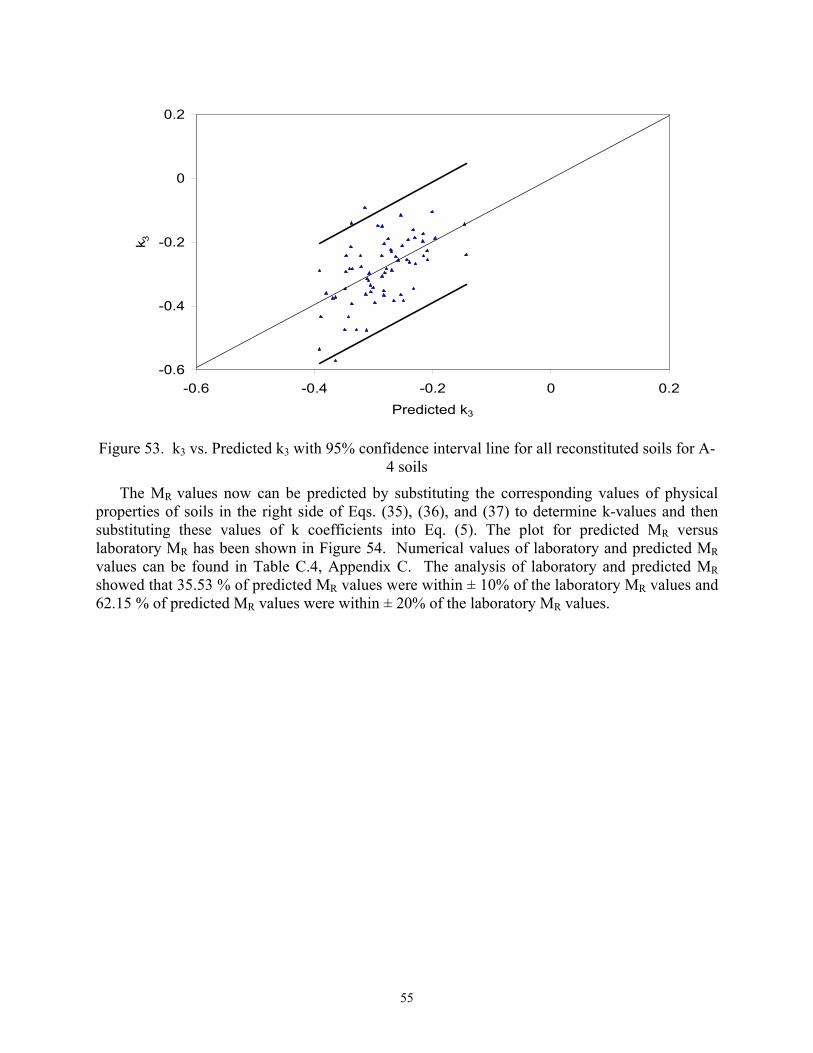
55

-0.6

-0.4

-0.2

0

0.2

-0.6 -0.4 -0.2 0 0.2Predicted k3

k 3


The MR values now can be predicted by substituting the corresponding values of physical properties of soils in the right side of Eqs. (35), (36), and (37) to determine k-values and then substituting these values of k coefficients into Eq. (5). The plot for predicted MR versus laboratory MR has been shown in Figure 54. Numerical values of laboratory and predicted MR values can be found in Table C.4, Appendix C. The analysis of laboratory and predicted MR showed that 35.53 % of predicted MR values were within ± 10% of the laboratory MR values and 62.15 % of predicted MR values were within ± 20% of the laboratory MR values.

56

0

50

100

150

200


Pre

dict

ed M

R (M

Pa)


• Samples compacted at optimum moisture content:

Regression equations developed for the k coefficients for the 41 samples from 13 different states compacted at optimum moisture content have been presented below (Eqs. (38), (39), and (40)).

log k1 = 3.60888 - 0.13212 x MC - 0.00161 x MAXDD + 0.02140 x S1_HALF - 0.01936 x S3_4 +

0.00790 x SN200 (R2 = 0.52; Adj. R2 = 0.45) (38) k2 = -3.29043 + 0.05316 x OMC + 0.00126 x DD - 0.00468 x PL + 0.01264 x S1 - 0.00819 x CSAND -

0.00295 x SILT - 0.01365 x CLAY (R2 = 0.68; Adj. R2 = 0.62) (39) k3 = 1.93886 - 0.05933 x MC - 0.00074630 x MAXDD - 0.00271x SN80 - 0.01004 x CSAND + 0.00420

x SILT (R2 = 0.50; Adj. R2 = 0.43) (40)

Plot for predicted MR calculated by substituting the values of k coefficients obtained by putting the values of the soil physical properties in Eqs. (38), (39), and (40) into Eq. (5), and laboratory MR has been presented in Figure 55. Numerical values of the predicted k coefficients can be found in Table D.16, Appendix D and numerical values for laboratory and predicted MR can be found in Table C.4, Appendix C. The analysis of laboratory and predicted MR showed that 35.83 % of predicted MR values were within ± 10% of the laboratory MR values and 66.29 % of predicted MR values were within ± 20% of the laboratory MR values.

57

0

50

100

150

200


Pre

dict

ed M

R (M

Pa)


content for A-4 soils • Samples compacted at insitu moisture content:

Prediction models for the A-4 soil samples compacted at insitu moisture content obtained after second step regression has been given below (Eqs. (41), (42), and (43)).

log k1 = 12.04783 - 0.06409 x MC - 0.06928 x OMC - 0.00152 x MAXDD - 0.12972 x S1 + 0.04723 x

S3_8 + 0.02535 x CLAY (R2 = 0.70; Adj. R2 = 0.60) (41)

k2 = 1.55793 - 0.00018031 x DD + 0.01067 x PL - 0.03284 x S3_8 + 0.04736 x SN10 - 0.02589 x SN80 - 0.02342 x CSAND (R2 = 0.77; Adj. R2 = 0.69) (42)

k3 = 3.18908 - 0.02399 x MC - 0.05290 x S1 + 0.02136 x SN4 + 0.00317 x CLAY (R2 = 0.42; Adj. R2 = 0.30) (43)

The plot for predicted MR values, obtained by substituting k coefficients from Eqs. (41), (42), and (43) into Eq. (5), against laboratory determined MR values has been shown in Figure 56. Numerical values of the predicted k coefficients can be found in Table D.16, Appendix D and numerical values for laboratory and predicted MR can be found in Table C.4, Appendix C. The analysis of laboratory and predicted MR showed that 39.04 % of predicted MR values were within ± 10% of the laboratory MR values and 73.79 % of predicted MR values were within ± 20% of the laboratory MR values.

58

0

50

100

150

200


Pre

dict

ed M

R (M

Pa)


A-4 soils 4.3.3.5. Soil Type: A-6

For regression to determine k coefficients of individual samples from known MR and stress values using Eq. (5), 40 soil specimens from 13 states in regions nearby the New England region were analyzed. Data for A-6 soil samples were not available in the LTPP database for the New England region. Since 1 sample resulted in positive k3 and 3 samples resulted in R2 less than 0.90 during this regression, these 4 samples were not used in the subsequent analysis to develop regression equations for predicting k coefficients in terms of physical soil properties for this soil type. Out of 36 specimens taken for second step regression, 23 samples had been compacted at optimum moisture content and 13 had been compacted at insitu moisture content. The regression equations for k1, k2, and k3 are given below:

• All reconstituted samples: The final regression equations for k1, k2, and k3 obtained from the second step regression

analysis for 36 reconstituted samples are as given below:

logk1 = 4.59815 – 0.12918 x MC – 0.00211x MAXDD + 0.04246 x LL – 0.0150 x CSAND – 0.01746 x CLAY (R2 = 0.52; Adj. R2 = 0.44) (44)

k2 = - 2.54229 + 0.00971 x MC + 0.00122 x MAXDD + 0.02703 x SN40 -0.02122 x SN200– 0.02393 x

FSAND (R2 = 0.47; Adj. R2 = 0.38) (45)

k3 = 2.08649 – 0.05214 x MC – 0.0007171x MAXDD + 0.02450 x LL - 0.01231 x S1 + 0.00493 x SN80 – 0.00922 x CLAY (R2 = 0.49; Adj. R2 = 0.38) (46)

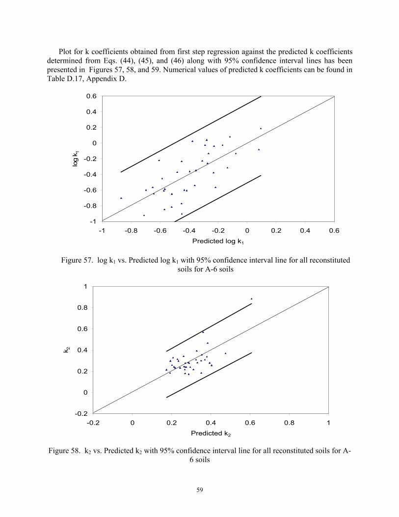
59

Plot for k coefficients obtained from first step regression against the predicted k coefficients determined from Eqs. (44), (45), and (46) along with 95% confidence interval lines has been presented in Figures 57, 58, and 59. Numerical values of predicted k coefficients can be found in Table D.17, Appendix D.

-1

-0.8

-0.6

-0.4

-0.2

0

0.2

0.4

0.6

-1 -0.8 -0.6 -0.4 -0.2 0 0.2 0.4 0.6Predicted log k1

log

k 1


-0.2

0

0.2

0.4

0.6

0.8

1

-0.2 0 0.2 0.4 0.6 0.8 1Predicted k2

k 2


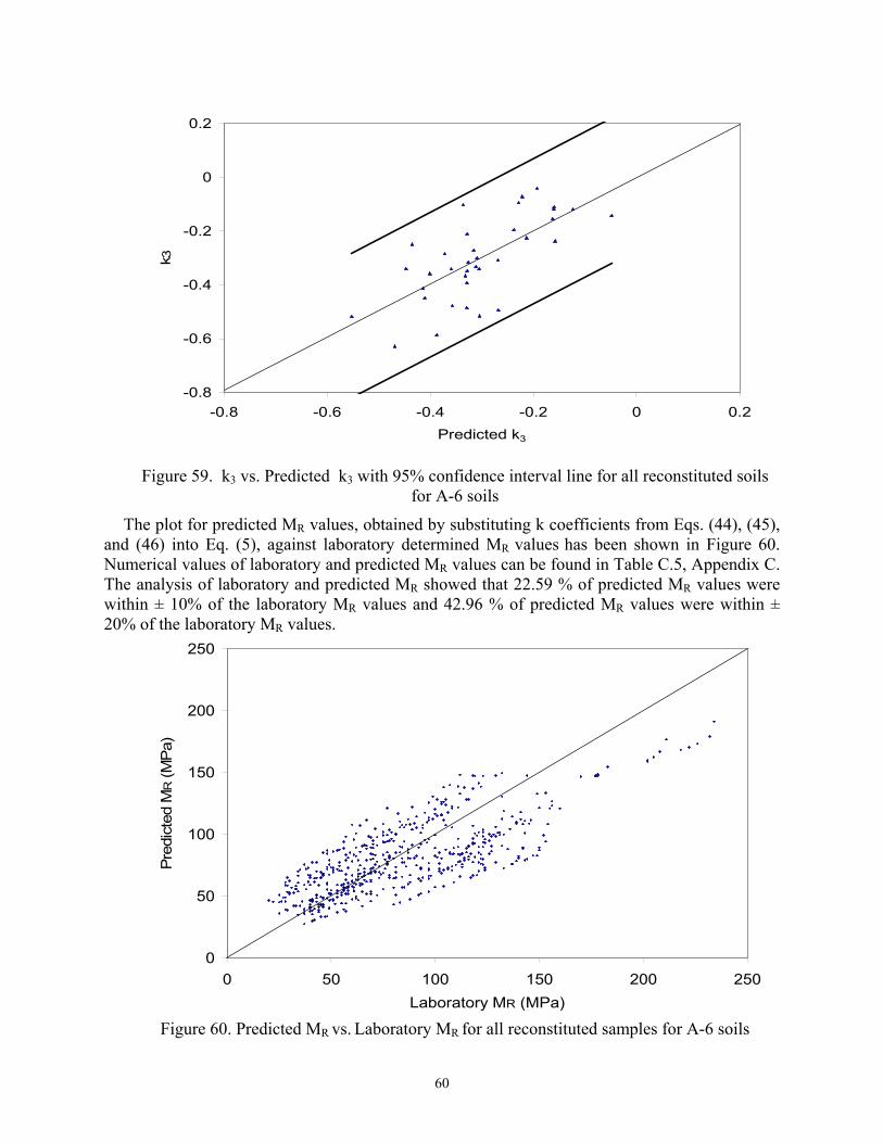
60

-0.8

-0.6

-0.4

-0.2

0

0.2

-0.8 -0.6 -0.4 -0.2 0 0.2Predicted k3

k 3


The plot for predicted MR values, obtained by substituting k coefficients from Eqs. (44), (45), and (46) into Eq. (5), against laboratory determined MR values has been shown in Figure 60. Numerical values of laboratory and predicted MR values can be found in Table C.5, Appendix C. The analysis of laboratory and predicted MR showed that 22.59 % of predicted MR values were within ± 10% of the laboratory MR values and 42.96 % of predicted MR values were within ± 20% of the laboratory MR values.

0

50

100

150

200

250

0 50 100 150 200 250Laboratory MR (MPa)

Pre

dict

ed M

R (M

Pa)


61

• Samples compacted at optimum moisture content: The regression equations for the k coefficients for 23 A-6 samples compacted at optimum

moisture content are as given in Eqs. (47), (48), and (49).

log k1 = 11.43172 - 0.11840 x MC + 0.07733 x PL + 0.03185 x LL - 0.16290 x S2 + 0.04052 x SN4 (R2 = 0.58; Adj. R2 = 0.45) (47)

k2 = - 3.39047 - 0.00037458 x MAXDD - 0.01423 x LL + 0.06384 x S2 - 0.01620 x SN4

(R2 = 0.45; Adj. R2 = 0.32) (48)

k3 = 5.70946 - 0.05880 x MC + 0.04341 x PL + 0.01976 x LL - 0.08633 x S2 + 0.02200 x SN4 (R2 = 0.55; Adj. R2 = 0.42) (49)

Figure 61 shows the plot of predicted MR obtained from the predicted k coefficients using Eqs. (47), (48), and (49) and laboratory measured MR values for the A-6 soil samples compacted at optimum moisture content. Numerical values of the predicted k coefficients can be found in Table D.17, Appendix D and numerical values for laboratory and predicted MR can be found in Table C.5, Appendix C. The analysis of laboratory and predicted MR showed that 33.62 % of predicted MR values were within ± 10% of the laboratory MR values and 57.10 % of predicted MR values were within ± 20% of the laboratory MR values.

0

50

100

150

200

250


Pred

icte

d M

R (M

Pa)

Figure 61. Predicted MR vs. Laboratory MR for soil samples compacted at optimum moisture

content for A-6 soils

• Samples compacted at insitu moisture content: Prediction models for the A-6 soil samples compacted at insitu moisture content obtained

after second step regression has been given below (Eqs. (50), (51), and (52)).

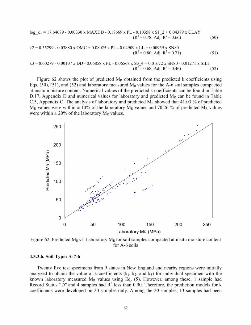
62

log_k1 = 17.64679 - 0.00330 x MAXDD - 0.17669 x PL - 0.10358 x S1_2 + 0.04379 x CLAY (R2 = 0.78; Adj. R2 = 0.66) (50)

k2 = 0.35299 - 0.03880 x OMC + 0.08025 x PL - 0.04909 x LL + 0.00939 x SN80 (R2 = 0.80; Adj. R2 = 0.71) (51)

k3 = 8.60279 - 0.00107 x DD - 0.06858 x PL - 0.06568 x S3_4 + 0.01672 x SN80 - 0.01271 x SILT (R2 = 0.68; Adj. R2 = 0.46) (52)

Figure 62 shows the plot of predicted MR obtained from the predicted k coefficients using

Eqs. (50), (51), and (52) and laboratory measured MR values for the A-6 soil samples compacted at insitu moisture content. Numerical values of the predicted k coefficients can be found in Table D.17, Appendix D and numerical values for laboratory and predicted MR can be found in Table C.5, Appendix C. The analysis of laboratory and predicted MR showed that 41.03 % of predicted MR values were within ± 10% of the laboratory MR values and 70.26 % of predicted MR values were within ± 20% of the laboratory MR values.

0

50

100

150

200

250


Pred

icte

d M

R (M

Pa)

Figure 62. Predicted MR vs. Laboratory MR for soil samples compacted at insitu moisture content

for A-6 soils

4.3.3.6. Soil Type: A-7-6

Twenty five test specimens from 9 states in New England and nearby regions were initially analyzed to obtain the value of k-coefficients (k1, k2, and k3) for individual specimen with the known laboratory measured MR values using Eq. (5). However, among these, 1 sample had Record Status “D” and 4 samples had R2 less than 0.90. Therefore, the prediction models for k coefficients were developed on 20 samples only. Among the 20 samples, 13 samples had been

63

compacted at optimum moisture content and 7 samples had been compacted at insitu moisture content. The results of second step regression to develop prediction models for k1, k2, and k3 have been presented below.


The regressions equations for k1, k2, and k3 for the 20 reconstituted samples are found as given below (Eqs. (53), (54), and (55)). log k1 = 6.54551 - 0.08119 x MC - 0.00202 x MAXDD - 0.00719 x PL - 0.01842 x SN200 - 0.06529 x

CSAND (R2 = 0.79; Adj. R2 = 0.72) (53) k2 = 9.78523 + 0.00743 x MC - 0.00018782 x DD - 0.01787 x LL - 0.08598 x S1_HALF (R2 = 0.45; Adj. R2 = 0.30) (54) k3 = 3.38876 - 0.03515 x MC - 0.00121 x MAXDD - 0.01073 x PL - 0.00711 x SN200 - 0.02667 x

CSAND (R2 = 0.70; Adj. R2 = 0.60) (55) Plot for k coefficients obtained from first step regression against the predicted k coefficients

determined from Eqs. (53), (54), and (55) along with 95% confidence interval lines has been presented in Figures 63, 64, and 65. Numerical values of predicted k coefficients can be found in Table D.18, Appendix D.

-2

-1.5

-1

-0.5

0

0.5

1

-2 -1.5 -1 -0.5 0 0.5 1Predicted logk1

log

k 1

Figure 63. log k1 vs. Predicted log k1 with 95% confidence interval line for all reconstituted soils for A-7-6 soils

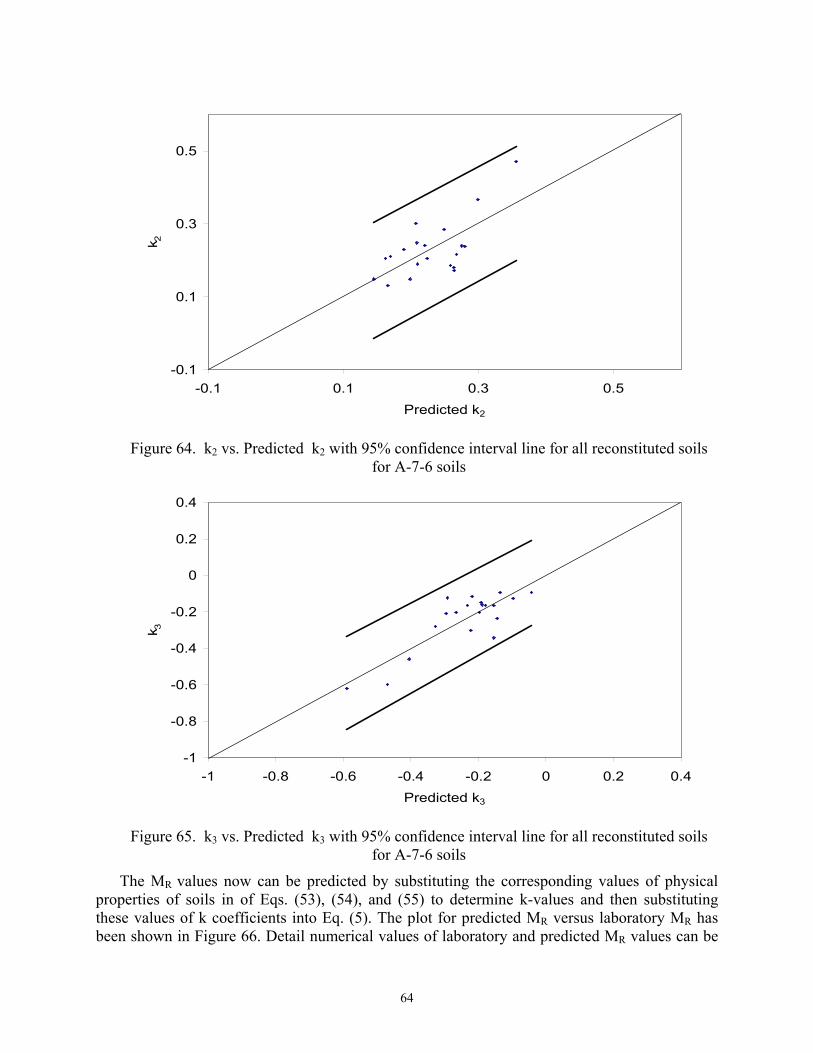
64

-0.1

0.1

0.3

0.5

-0.1 0.1 0.3 0.5Predicted k2

k 2


-1

-0.8

-0.6

-0.4

-0.2

0

0.2

0.4

-1 -0.8 -0.6 -0.4 -0.2 0 0.2 0.4Predicted k3

k 3


The MR values now can be predicted by substituting the corresponding values of physical properties of soils in of Eqs. (53), (54), and (55) to determine k-values and then substituting these values of k coefficients into Eq. (5). The plot for predicted MR versus laboratory MR has been shown in Figure 66. Detail numerical values of laboratory and predicted MR values can be

65

found in Table C.6, Appendix C. The analysis of laboratory and predicted MR showed that 36.33 % of predicted MR values were within ± 10% of the laboratory MR values and 66.33 % of predicted MR values were within ± 20% of the laboratory MR values.

0

50

100

150

200

250


Pred

icte

d M

R (M

Pa)

Figure 66. Predicted MR vs. Laboratory MR for all reconstituted samples for A-7-6 soils

• Samples compacted at optimum moisture content: Regression equations developed for the k coefficients for the 13 samples from 7 different

states compacted at optimum moisture content have been presented below (Eqs. (56), (57), and (58)). log k1 = 4.52887 + 0.05361 x OMC + 0.00223 x DD - 7.51558 x DDR - 0.01658 x SN4 - 0.01507 x

CLAY (R2 = 0.82; Adj. R2 = 0.70) (56) k2 = -1.25242 + 0.01445 x OMC + 0.00092437 x MAXDD - 0.00610 x FSAND - 0.00825 x CLAY (R2 = 0.80; Adj. R2 = 0.70) (57) k3 = 1.12933 + 0.02765 x OMC + 0.00104 x DD - 3.32254 x DDR - 0.00902 x CLAY (R2 = 0.62; Adj. R2 = 0.43) (58)

Plot for predicted MR calculated by substituting the values of k coefficients obtained by putting the values of the soil physical properties in Eqs. (56), (57), and (58) into Eq. (5) and laboratory MR has been presented in Figure 67. Numerical values of the predicted k coefficients can be found in Table D.18, Appendix D and numerical values for laboratory and predicted MR can be found in Table C.6, Appendix C. The analysis of laboratory and predicted MR showed that 67.18 % of predicted MR values were within ± 10% of the laboratory MR values and 95.38 % of predicted MR values were within ± 20% of the laboratory MR values.

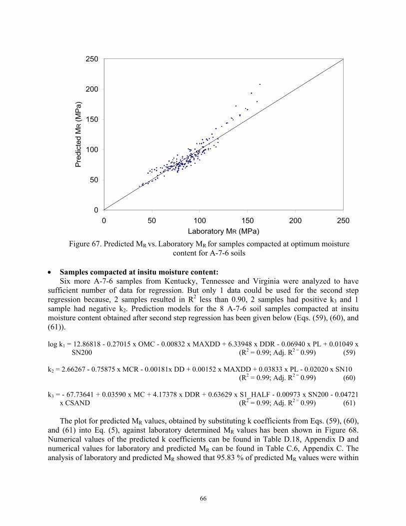
66

0

50

100

150

200

250


Pred

icte

d M

R (M

Pa)


content for A-7-6 soils • Samples compacted at insitu moisture content:

Six more A-7-6 samples from Kentucky, Tennessee and Virginia were analyzed to have sufficient number of data for regression. But only 1 data could be used for the second step regression because, 2 samples resulted in R2 less than 0.90, 2 samples had positive k3 and 1 sample had negative k2. Prediction models for the 8 A-7-6 soil samples compacted at insitu moisture content obtained after second step regression has been given below (Eqs. (59), (60), and (61)).

log k1 = 12.86818 - 0.27015 x OMC - 0.00832 x MAXDD + 6.33948 x DDR - 0.06940 x PL + 0.01049 x

SN200 (R2 = 0.99; Adj. R2 = 0.99) (59)

k2 = 2.66267 - 0.75875 x MCR - 0.00181x DD + 0.00152 x MAXDD + 0.03833 x PL - 0.02020 x SN10 (R2 = 0.99; Adj. R2 = 0.99) (60)

k3 = - 67.73641 + 0.03590 x MC + 4.17378 x DDR + 0.63629 x S1_HALF - 0.00973 x SN200 - 0.04721

x CSAND (R2 = 0.99; Adj. R2 = 0.99) (61)

The plot for predicted MR values, obtained by substituting k coefficients from Eqs. (59), (60), and (61) into Eq. (5), against laboratory determined MR values has been shown in Figure 68. Numerical values of the predicted k coefficients can be found in Table D.18, Appendix D and numerical values for laboratory and predicted MR can be found in Table C.6, Appendix C. The analysis of laboratory and predicted MR showed that 95.83 % of predicted MR values were within

67

± 10% of the laboratory MR values and 100 % of predicted MR values were within ± 20% of the laboratory MR values.

0

50

100

150

200

250


Pred

icte

d M

R (M

Pa)


A-7-6 soils 4.4 Limits of Soil Properties Values used in Second Step Regression Analysis for AASHTO Soil Types

A regression model is simply a fit to a database of observed responses. Hence, it should not be trusted to make predictions outside the range of the predictor/regressor variables used in fitting the model. Therefore, the first step in predicting values from regression model should be to verify that the prediction does not require extrapolation beyond the range of the regressor variables in the original data set (Rauch 1997). Attempting to use a regression equation beyond the range of the regressor variables is often inappropriate and may yield incredible answers (www.state.yale.edu).

The minimum and maximum of the soil properties values used in the second step regression

analysis have been presented in Table 16. Designations MODEL1, MODEL2, and MODEL3 have been used for model containing all reconstituted samples, model containing samples compacted near to optimum moisture content only, and model containing samples compacted near to insitu moisture content only respectively.

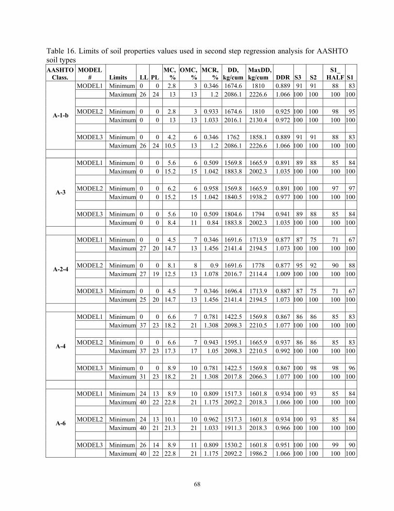
68

Table 16. Limits of soil properties values used in second step regression analysis for AASHTO soil types AASHTO

Class. MODEL

# Limits LL PL MC,

% OMC,

%MCR,

% DD,

kg/cum MaxDD, kg/cum DDR S3 S2

S1_ HALF S1

MODEL1 Minimum 0 0 2.8 3 0.346 1674.6 1810 0.889 91 91 88 83 Maximum 26 24 13 13 1.2 2086.1 2226.6 1.066 100 100 100 100

MODEL2 Minimum 0 0 2.8 3 0.933 1674.6 1810 0.925 100 100 98 95 Maximum 0 0 13 13 1.033 2016.1 2130.4 0.972 100 100 100 100

MODEL3 Minimum 0 0 4.2 6 0.346 1762 1858.1 0.889 91 91 88 83

A-1-b

Maximum 26 24 10.5 13 1.2 2086.1 2226.6 1.066 100 100 100 100

MODEL1 Minimum 0 0 5.6 6 0.509 1569.8 1665.9 0.891 89 88 85 84 Maximum 0 0 15.2 15 1.042 1883.8 2002.3 1.035 100 100 100 100


MODEL3 Minimum 0 0 5.6 10 0.509 1804.6 1794 0.941 89 88 85 84

A-3

Maximum 0 0 8.4 11 0.84 1883.8 2002.3 1.035 100 100 100 100


MODEL2 Minimum 0 0 8.1 8 0.9 1691.6 1778 0.877 95 92 90 88 Maximum 27 19 12.5 13 1.078 2016.7 2114.4 1.009 100 100 100 100

MODEL3 Minimum 0 0 4.5 7 0.346 1696.4 1713.9 0.887 87 75 71 67

A-2-4

Maximum 25 20 14.7 13 1.456 2141.4 2194.5 1.073 100 100 100 100



MODEL3 Minimum 0 0 8.9 10 0.781 1422.5 1569.8 0.867 100 98 98 96

A-4

Maximum 31 23 18.2 21 1.308 2017.8 2066.3 1.077 100 100 100 100



MODEL3 Minimum 26 14 8.9 11 0.809 1530.2 1601.8 0.951 100 100 99 90

A-6

Maximum 40 22 22.8 21 1.175 2092.2 1986.2 1.066 100 100 100 100

69

Table 16. Limits of soil properties values used in second step regression analysis for AASHTO soil types (Cont’d…) AASHTO

Class. MODEL

# Limits S3_4 S1_2 S3_8 SN4 SN10 SN40 SN80 SN200 CSAND FSAND SILT CLAYMODEL1 Minimum 76 67 61 50 41 26 3 1.4 6 10 0.6 0 Maximum 100 100 99 98 95 72 38 26.4 48 69 17.6 8.6

MODEL2 Minimum 91 78 70 57 48 26 3 1.4 6 25 0.6 0.2 Maximum 100 100 99 98 95 49 32 21.7 46 56 14.9 4.7

MODEL3 Minimum 76 67 61 50 41 26 7 3.8 8 10 1.3 0

A-1-b

Maximum 100 100 99 97 95 72 38 26.4 48 69 17.6 8.6

MODEL1 Minimum 83 82 82 81 76 53 8 1.9 2 45 1.8 0 Maximum 100 100 100 100 100 98 57 9.6 34 94 10 6.3

MODEL2 Minimum 96 95 93 91 87 53 8 1.9 2 46 1.8 0 Maximum 100 100 100 100 100 98 57 9.1 34 94 10 6.3

MODEL3 Minimum 83 82 82 81 76 54 9 3.9 19 45 3 1.3

A-3

Maximum 100 100 100 99 97 72 24 9.6 26 69 6.1 3.5



MODEL3 Minimum 63 57 53 47 40 33 19 5.5 2 4 4.7 2.3

A-2-4

Maximum 100 100 100 100 100 98 75 33.8 24 85 24.6 24.6

MODEL1 Minimum 80 76 74 69 60 48 42 35.2 0 1 21.5 2.8 Maximum 100 100 100 100 100 99 99 98 36 57 87.2 32.2


MODEL3 Minimum 94 90 87 83 80 62 48 40.5 0 1 25.5 2.8

A-4

Maximum 100 100 100 100 100 99 99 98 36 50 87.2 32.2



MODEL3 Minimum 88 83 79 70 62 53 48 43 0 1 32.3 12.1

A-6

Maximum 100 100 100 100 100 99 98 97.5 13 30 70.3 31.1

70

Table 16. Limits of soil properties values used in second step regression analysis for AASHTO soil types (Cont’d…) AASHTO

Class. MODEL

# Limits LL PL MC, %

OMC, %

MCR, %

DD, kg/cum

MaxDD, kg/cum DDR S3 S2

S1_ HALF S1

MODEL1 Minimum 41 15 12.9 13 0.974 1463.8 1473.7 0.888 100 97 95 93 Maximum 68 27 30.7 27 1.289 1780.1 1810 1.029 100 100 100 100

MODEL2 Minimum 41 15 12.9 13 0.974 1490.4 1569.8 0.929 100 97 95 93 Maximum 68 27 22.5 22 1.028 1721.8 1810 1.002 100 100 100 100

MODEL3 Minimum 41 17 16.6 16 1.038 1463.8 1473.7 0.888 100 100 99 98

A-7-6

Maximum 57 24 30.7 27 1.335 1780.1 1729.9 1.029 100 100 100 100 Table 16. Limits of soil properties values used in second step regression analysis for AASHTO soil types (Cont’d…) AASHTO

Class. MODEL

# Limits S3_4 S1_2 S3_8 SN4 SN10 SN40 SN80 SN200 CSAND FSAND SILTCLAYMODEL1 Minimum 91 88 85 78 70 59 55 51 0 1 14.8 24.2

Maximum 100 100 100 100 100 99 99 98.6 13 28 71.7 58.5


MODEL3 Minimum 94 92 91 88 85 78 63 51 1 1 23.9 25.1

A-7-6

Maximum 100 100 100 100 100 99 97 96.7 13 24 71.7 58.5

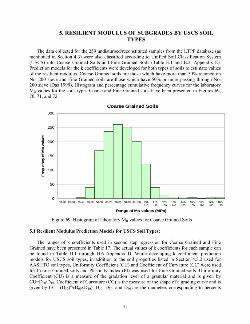
71

5. RESILIENT MODULUS OF SUBGRADES BY USCS SOIL TYPES

The data collected for the 259 undisturbed/reconstituted samples from the LTPP database (as

mentioned in Section 4.3) were also classified according to Unified Soil Classification System (USCS) into Coarse Grained Soils and Fine Grained Soils (Table E.1 and E.2, Appendix E). Prediction models for the k coefficients were developed for both types of soils to estimate values of the resilient modulus. Coarse Grained soils are those which have more than 50% retained on No. 200 sieve and Fine Grained soils are those which have 50% or more passing through No. 200 sieve (Das 1999). Histogram and percentage cumulative frequency curves for the laboratory MR values for the soils types Coarse and Fine Grained soils have been presented in Figures 69, 70, 71, and 72.

Coarse Grained Soils

0

50

100

150

200

250

300

10-20 20-30 30-40 40-50 50-60 60-70 70-80 80-90 90-100 100-110

110-120

120-130

130-140

140-150

150-160

160-170

170-180

180-190


Freq

uenc

y of

M R

valu

es

Figure 69. Histogram of laboratory MR values for Coarse Grained Soils

5.1 Resilient Modulus Prediction Models for USCS Soil Types:

The ranges of k coefficients used in second step regression for Coarse Grained and Fine Grained have been presented in Table 17. The actual values of k coefficients for each sample can be found in Table D.1 through D.6 Appendix D. While developing k coefficient prediction models for USCS soil types, in addition to the soil properties listed in Section 4.3.2 used for AASHTO soil types, Uniformity Coefficient (CU) and Coefficient of Curvature (CC) were used for Coarse Grained soils and Plasticity Index (PI) was used for Fine Grained soils. Uniformity Coefficient (CU) is a measure of the gradation level of a granular material and is given by CU=D60/D10. Coefficient of Curvature (CC) is the measure of the shape of a grading curve and is given by CC= (D30)2/(D60xD10). D10, D30, and D60 are the diameters corresponding to percents

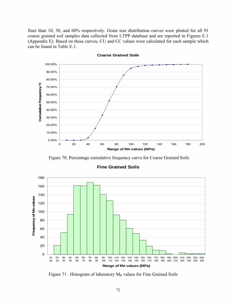
72

finer than 10, 30, and 60% respectively. Grain size distribution curves were plotted for all 91 coarse grained soil samples data collected from LTPP database and are reported in Figures E.1 (Appendix E). Based on these curves, CU and CC values were calculated for each sample which can be found in Table E.1.

Coarse Grained Soils

0.00%

10.00%

20.00%

30.00%

40.00%

50.00%

60.00%

70.00%

80.00%

90.00%

100.00%

0 20 40 60 80 100 120 140 160 180 200


Cum

ulat

ive

Freq

uenc

y %

Figure 70. Percentage cumulative frequency curve for Coarse Grained Soils

Fine Grained Soils

0

20

40

60

80

100

120

140

160

180

10-20

20-30

30-40

40-50

50-60

60-70

70-80

80-90

90-100

100-110

110-120

120-130

130-140

140-150

150-160

160-170

170-180

180-190

190-200

200-210

210-220

220-230

230-240

240-250


Freq

uenc

y of

M R

valu

es

Figure 71 . Histogram of laboratory MR values for Fine Grained Soils

73

Fine Grained Soils

0.00%

10.00%

20.00%

30.00%

40.00%

50.00%

60.00%

70.00%

80.00%

90.00%

100.00%

0 20 40 60 80 100 120 140 160 180 200 220 240 260


Cum

ulat

ive

Freq

uenc

y %

Figure 72. Percentage cumulative frequency curve for Fine Grained Soils

Table 17. Range of k coefficients for Coarse Grained and Fine Grained soils used in second step regression

USCS Soil Type Variable No. of Samples


Minimum Maximum

k1 91 0.46610 0.10443 0.21628 1.01422 k2 91 0.65136 0.11869 0.28572 0.88301

Coarse Grained (All Samples)

k3 91 -0.16708 0.08480 -0.41500 -0.00894k1 74 0.46977 0.08053 0.21628 0.68305 k2 74 0.67972 0.09555 0.45572 0.88301

Coarse Grained (Samples with CU≤100

only) k3 74 -0.14326 0.06356 -0.41500 -0.00894k1 97 0.48174 0.30195 0.06643 1.53817 k2 97 0.33366 0.14950 0.13053 0.98855

Fine Grained

k3 97 -0.29013 0.13991 -0.62807 -0.03903 5.1.1 USCS Soil Type: Coarse Grained

Ninety one soil samples were available for second step regression for the coarse grained soils after screening for samples with R2 less than 0.90, samples with negative k1 and k2 and positive k3. It can be observed from the histogram of CU values (Figure 73) that the majority (81.3%) of coarse grained soils had Uniformity Coefficient (CU) values less than 100. Therefore, two sets of models have been developed for coarse grained soils. The first set of model has all samples extracted from the LTPP database that fall in coarse grained criteria. The second set of model

74

were developed incorporating only those soil samples which had CU≤100 to avoid possible influence of some extreme values of CU on the prediction models. Histogram of CU values for coarse grained soil samples with CU≤100 has been presented in Figure 74. It can be seen from Figure 74 that the majority of samples have CU<10.

0

10

20

30

40

50

60

70

80

0-10

0

200-

300

400-

500

600-

700

800-

900

1000

-110

0

1200

-130

0

1400

-150

0

1600

-170

0

1800

-190

0

2000

-210

0

2200

-230

0

2400

-250

0

2600

-270

0

2800

-290

0

3000

-310

0

3200

-330

0

3400

-350

0

3600

-370

0

3800

-390

0

4000

-410

0

Range of CU values

Freq

uenc

y of

C U

val

ue

Figure 73. Histogram of CU values for all Coarse Grained Soils

• All Coarse Grained samples: Regression equations developed for k coefficients from 91 coarse grained soils have been

presented below along with the R2 values for each equation.

log k1 = -1.77341 + 0.00017562 x MAXDD + 0.02707 x S3 - 0.02043 x S1 + 0.00501 x S3_8 - 0.00819 x SN200 + 0.00501 x SILT (R2 = 0.40; Adj. R2 = 0.36) (62)

k2 = -0.49426 + 0.11250 x MCR + 0.00026190 x DD + 0.00592 x S3 - 0.00398 x SN40 + 0.00479 x

FSAND - 0.00006099 x CU - 0.0000967 x CC (R2 = 0.45; Adj. R2 = 0.41) (63) k3 = -0.44082 - 0.00232 x MC + 0.00021026 x MAXDD - 0.00531 x S1_2 + 0.00561 x SN10 - 0.00529 x

SN200 (R2 = 0.63; Adj. R2 = 0.61) (64)

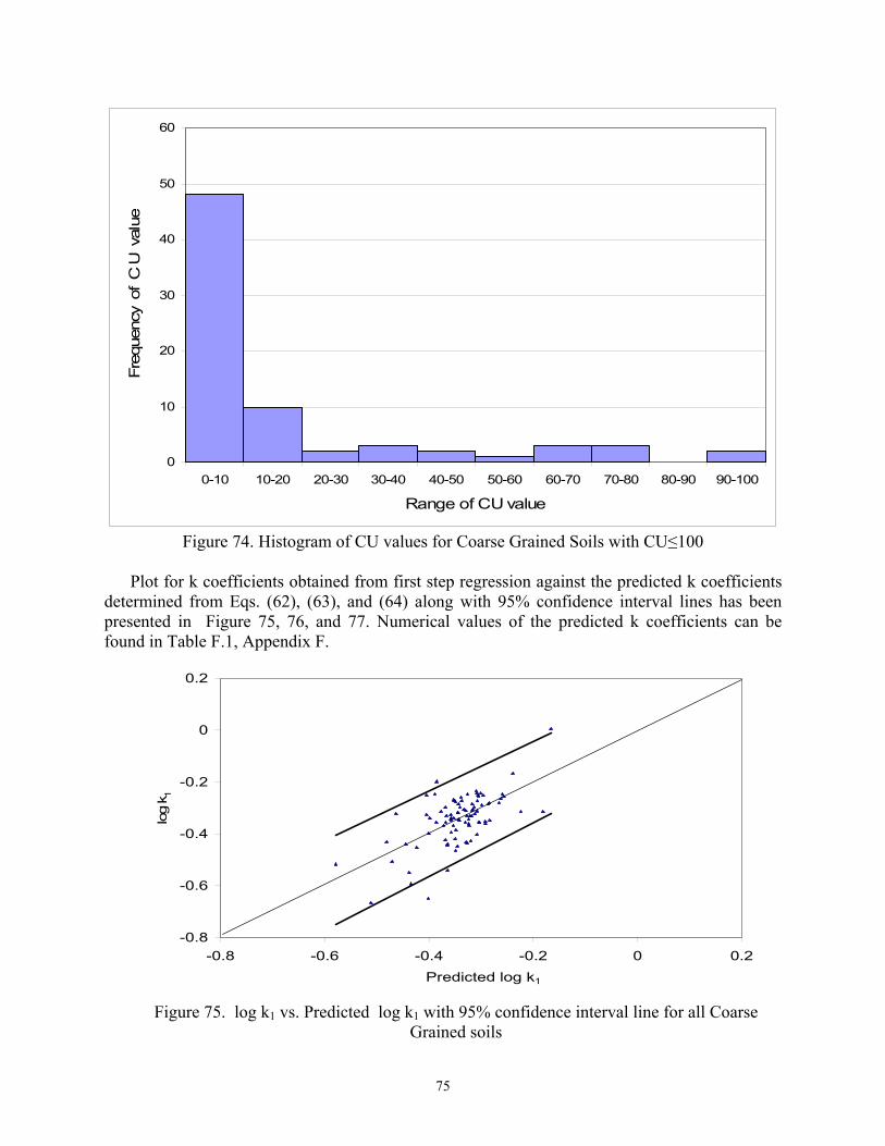
75

0

10

20

30

40

50

60

0-10 10-20 20-30 30-40 40-50 50-60 60-70 70-80 80-90 90-100

Range of CU value

Freq

uenc

y o

f C

U v

alue

Figure 74. Histogram of CU values for Coarse Grained Soils with CU≤100

Plot for k coefficients obtained from first step regression against the predicted k coefficients determined from Eqs. (62), (63), and (64) along with 95% confidence interval lines has been presented in Figure 75, 76, and 77. Numerical values of the predicted k coefficients can be found in Table F.1, Appendix F.

-0.8

-0.6

-0.4

-0.2

0

0.2

-0.8 -0.6 -0.4 -0.2 0 0.2 Predicted log k1

log

k 1

Figure 75. log k1 vs. Predicted log k1 with 95% confidence interval line for all Coarse Grained soils

76

0

0.2

0.4

0.6

0.8

1

0 0.2 0.4 0.6 0.8 1 Predicted k2

k 2

Figure 76. k2 vs. Predicted k2 with 95% confidence interval line for all Coarse Grained soils

-0.6

-0.4

-0.2

0

0.2

-0.6 -0.4 -0.2 0 0.2 Predicted k3

k 3

Figure 77. k3 vs. Predicted k3 with 95% confidence interval line for all Coarse Grained soils

Plot for predicted MR calculated by substituting values of k1, k2, and k3 obtained from Eqs.

(62), (63), and (64) into Eq. (5) against laboratory MR has been presented in Figure 78. Numerical values of laboratory and predicted MR can be found in Table F.3, Appendix F. Analysis of predicted and laboratory MR values showed that 50.04% and 77.63% of predicted MR were within ± 10% and ± 20% respectively, of laboratory MR.

77

0

50

100

150

200


Pred

icte

d M

R (M

Pa)

Figure 78. Predicted MR vs. Laboratory MR for all Coarse Grained soils

• Coarse Grained samples with CU≤100: Prediction models for k coefficients developed from 74 coarse grained soil samples that had

CU≤100 have been presented in Eqs. (65), (66), and (67).

log k1 = 0.61689 - 0.00815 x OMC - 0.06144 x MCR - 0.80003 x DDR - 0.00878 x SN200 + 0.00624 x SILT + 0.00621 x CLAY - 0.00502 x CC (R2 = 0.47; Adj. R2 = 0.41) (65)

k2 = 0.43372 + 0.00687 x MC + 0.00039979 x DD - 0.00026666 x MAXDD - 0.00331 x SN40 + 0.00297

x FSAND + 0.00515 x CC (R2 = 0.22; Adj. R2 = 0.15) (66) k3 = 0.51731 - 0.00390 x MC - 0.43830 x DDR - 0.00594 x S1_2 + 0.00509 x SN10 - 0.00070032 x

SN40 - 0.00418 x SN200 + 0.00441 x CLAY (R2 = 0.52; Adj. R2 = 0.47) (67)

Numerical values of predicted k coefficients can be found in Table F.1, Appendix F and numerical values of laboratory and predicted MR can be found in Table F.3, Appendix F. Plot for predicted MR versus laboratory MR has been presented in Figure 79. The analysis of predicted and laboratory MR showed that 60.32% and 85.75% of predicted MR values were within ±10% and ± 20% respectively, of the laboratory MR values.

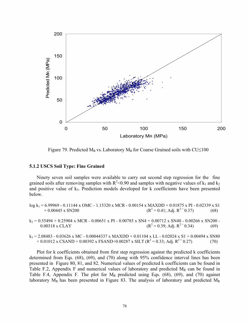
78

0

50

100

150

200


Pred

icte

d M

R (M

Pa)

Figure 79. Predicted MR vs. Laboratory MR for Coarse Grained soils with CU≤100 5.1.2 USCS Soil Type: Fine Grained

Ninety seven soil samples were available to carry out second step regression for the fine grained soils after removing samples with R2<0.90 and samples with negative values of k1 and k2 and positive value of k3. Prediction models developed for k coefficients have been presented below.

log k1 = 6.99969 - 0.11144 x OMC - 1.15320 x MCR - 0.00154 x MAXDD + 0.01875 x PI - 0.02339 x S1

+ 0.00445 x SN200 (R2 = 0.41; Adj. R2 = 0.37) (68) k2 = 0.55494 + 0.25904 x MCR - 0.00651 x PI - 0.00785 x SN4 + 0.00712 x SN40 - 0.00266 x SN200 -

0.00318 x CLAY (R2 = 0.39; Adj. R2 = 0.34) (69) k3 = 2.08483 - 0.03626 x MC - 0.00044337 x MAXDD + 0.01104 x LL - 0.02024 x S1 + 0.00494 x SN80

+ 0.01012 x CSAND + 0.00392 x FSAND+0.00287 x SILT (R2 = 0.33; Adj. R2 = 0.27) (70)

Plot for k coefficients obtained from first step regression against the predicted k coefficients determined from Eqs. (68), (69), and (70) along with 95% confidence interval lines has been presented in Figure 80, 81, and 82. Numerical values of predicted k coefficients can be found in Table F.2, Appendix F and numerical values of laboratory and predicted MR can be found in Table F.4, Appendix F. The plot for MR predicted using Eqs. (68), (69), and (70) against laboratory MR has been presented in Figure 83. The analysis of laboratory and predicted MR

79

showed that 30.03% of predicted MR were within ± 10% of laboratory MR and 50.86% of predicted MR were within ± 20% of the laboratory MR.

-1.6

-1.4

-1.2

-1

-0.8

-0.6

-0.4

-0.2

0

0.2

0.4

0.6

0.8

-1.6 -1.4 -1.2 -1 -0.8 -0.6 -0.4 -0.2 0 0.2 0.4 0.6 0.8 Predicted log k1

log

k 1

Figure 80. log k1 vs. Predicted log k1 with 95% confidence interval line for Fine Grained soils

-0.2

0

0.2

0.4

0.6

0.8

1

-0.2 0 0.2 0.4 0.6 0.8 1 Predicted k2

k 2

Figure 81. k2 vs. Predicted k2 with 95% confidence interval line for Fine Grained soils

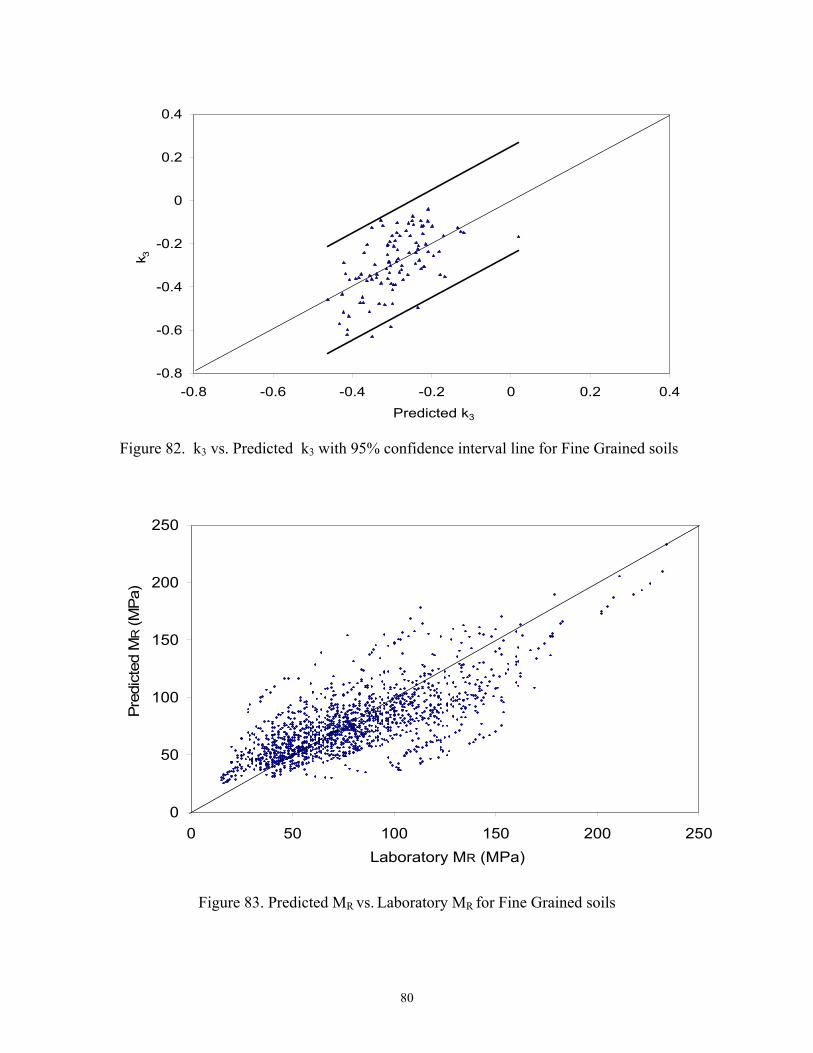
80

-0.8

-0.6

-0.4

-0.2

0

0.2

0.4

-0.8 -0.6 -0.4 -0.2 0 0.2 0.4 Predicted k3

k 3

Figure 82. k3 vs. Predicted k3 with 95% confidence interval line for Fine Grained soils

0

50

100

150

200

250


Pred

icte

d M

R (M

Pa)

Figure 83. Predicted MR vs. Laboratory MR for Fine Grained soils

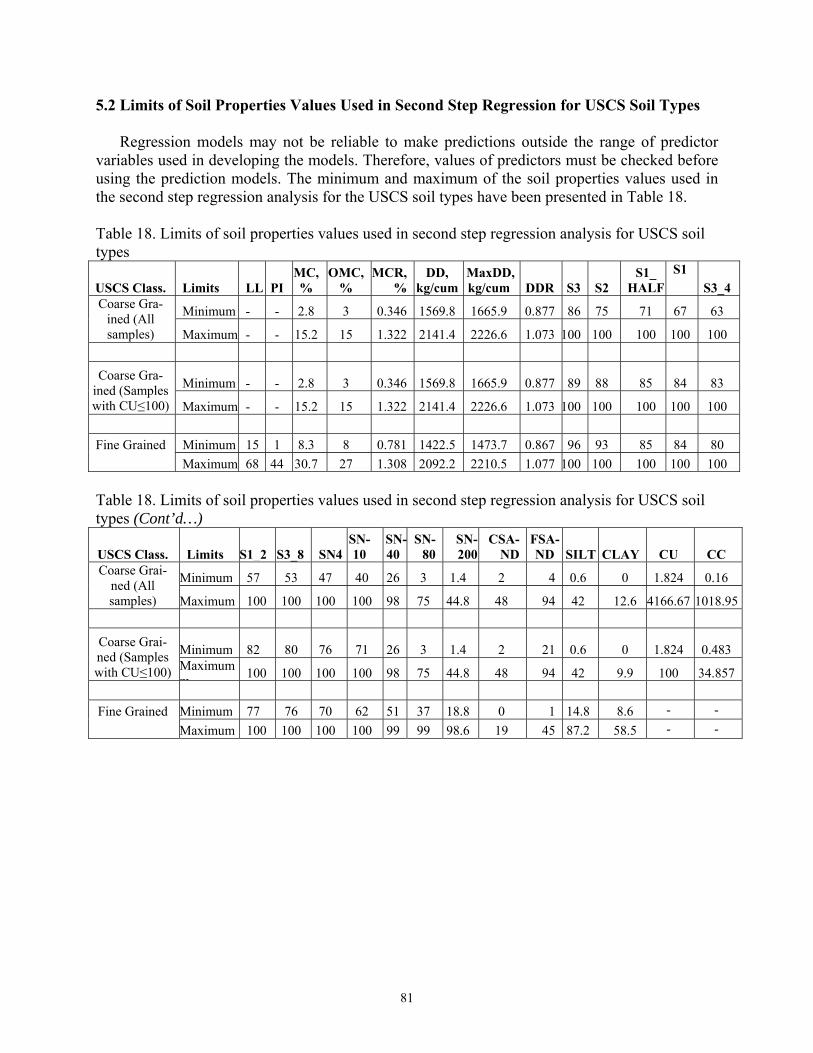
81

5.2 Limits of Soil Properties Values Used in Second Step Regression for USCS Soil Types

Regression models may not be reliable to make predictions outside the range of predictor variables used in developing the models. Therefore, values of predictors must be checked before using the prediction models. The minimum and maximum of the soil properties values used in the second step regression analysis for the USCS soil types have been presented in Table 18. Table 18. Limits of soil properties values used in second step regression analysis for USCS soil types

USCS Class. Limits LL PI MC, %

OMC, %

MCR, %

DD, kg/cum

MaxDD, kg/cum DDR S3 S2

S1_ HALF

S1 S3_4

Minimum - - 2.8 3 0.346 1569.8 1665.9 0.877 86 75 71 67 63 Coarse Gra-ined (All samples) Maximum - - 15.2 15 1.322 2141.4 2226.6 1.073 100 100 100 100 100

Minimum - - 2.8 3 0.346 1569.8 1665.9 0.877 89 88 85 84 83 Coarse Gra-ined (Samples with CU≤100) Maximum - - 15.2 15 1.322 2141.4 2226.6 1.073 100 100 100 100 100

Fine Grained Minimum 15 1 8.3 8 0.781 1422.5 1473.7 0.867 96 93 85 84 80

Maximum 68 44 30.7 27 1.308 2092.2 2210.5 1.077 100 100 100 100 100 Table 18. Limits of soil properties values used in second step regression analysis for USCS soil types (Cont’d…)

USCS Class. Limits S1_2 S3_8 SN4SN- 10

SN-40

SN-80

SN-200

CSA-ND

FSA-ND SILT CLAY CU CC

Minimum 57 53 47 40 26 3 1.4 2 4 0.6 0 1.824 0.16 Coarse Grai-ned (All samples) Maximum 100 100 100 100 98 75 44.8 48 94 42 12.6 4166.67 1018.95

Minimum 82 80 76 71 26 3 1.4 2 21 0.6 0 1.824 0.483 Coarse Grai-ned (Samples with CU≤100) Maximum

m 100 100 100 100 98 75 44.8 48 94 42 9.9 100 34.857

Fine Grained Minimum 77 76 70 62 51 37 18.8 0 1 14.8 8.6 - - Maximum 100 100 100 100 99 99 98.6 19 45 87.2 58.5 - -

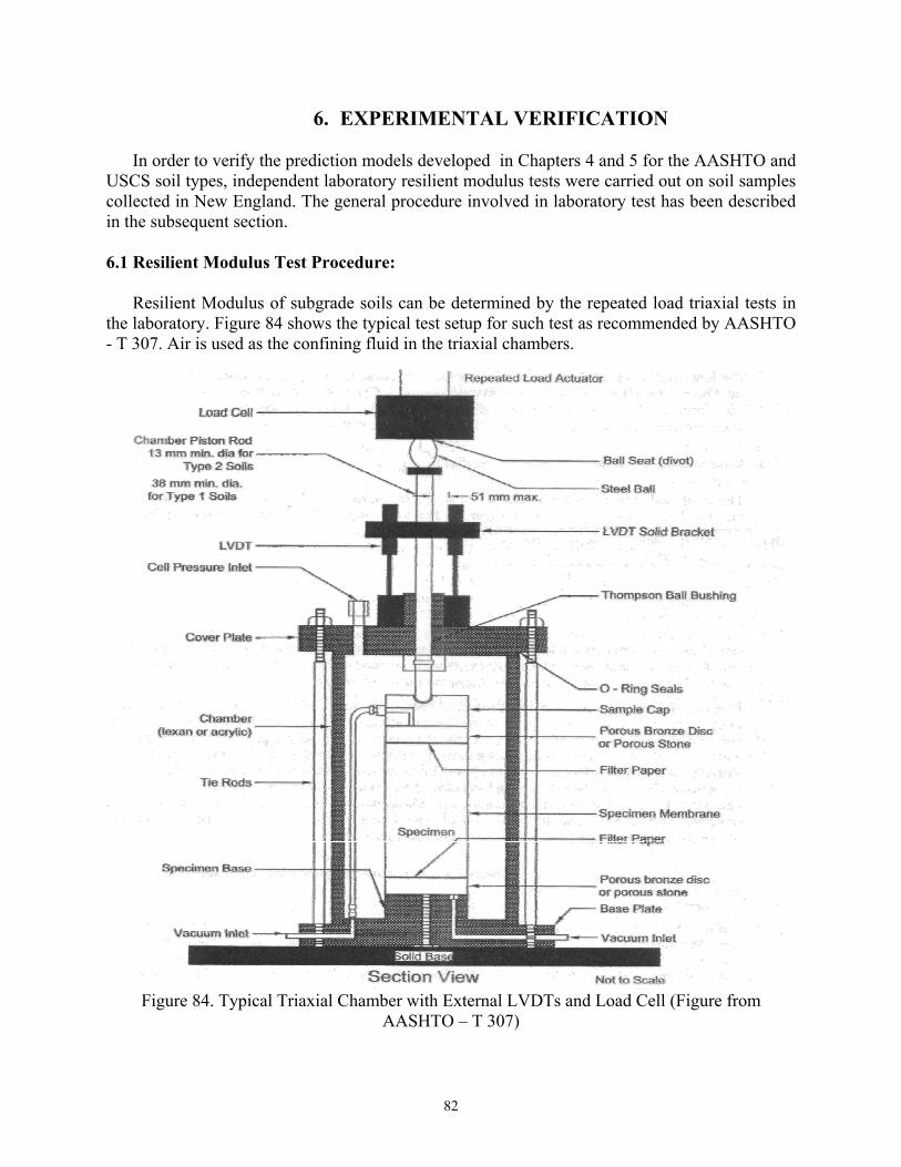
82

6. EXPERIMENTAL VERIFICATION

In order to verify the prediction models developed in Chapters 4 and 5 for the AASHTO and USCS soil types, independent laboratory resilient modulus tests were carried out on soil samples collected in New England. The general procedure involved in laboratory test has been described in the subsequent section.

6.1 Resilient Modulus Test Procedure:

Resilient Modulus of subgrade soils can be determined by the repeated load triaxial tests in the laboratory. Figure 84 shows the typical test setup for such test as recommended by AASHTO - T 307. Air is used as the confining fluid in the triaxial chambers.

Figure 84. Typical Triaxial Chamber with External LVDTs and Load Cell (Figure from

AASHTO – T 307)

83

A repeated axial cyclic stress (Scyclic) of fixed magnitude is applied to a cylindrical test specimen using a haversine-shaped load pulse with load duration (0.1s), and cycle duration (1.0 to 3.1 s) as shown in Figure 85. The test specimen is subjected to the dynamic cyclic stress (Scyclic) and a static confining stress provided by means of a triaxial pressure. For subgrade soils, each soil specimen is tested at 3 levels of confining pressure (41.4, 27.8, and 13.8 kPa). At each level of confining pressure 5 levels of cyclic stress are applied. At the end of each loading cycle deformation is measured externally with the 2 spring-loaded Linear Variable Differential Transducers (LVDT) as shown in Figure 84. Resilient modulus (MR) is calculated as follows:

MR = Scyclic / εr …………………………………………………….. (71)

where, Scyclic = cyclic applied axial stress εr = resilient recovered axial strain= er / L where, er = resilient (recovered) axial deformation due to Scyclic; L = original specimen length

Hence, each MR test results in 15 values of MR at 15 different combinations of stresses.

Figure 85. Haversine shaped load pulse used in resilient modulus testing (Figure from AASHTO

– T 307)

6.2 Soil Samples Data Collected in New England

Laboratory tests were carried out at the Braun Intertec Corporation, Minneapolis, MN on soil types A-1-b, A-3, A-2-4, A-4, and A-7-6 collected in New England. A-6 soil was not present

84

among the soil samples collected so prediction models for this soil type could not be verified. The laboratory tests include repeated load tests for resilient modulus (MR), determination of moisture content and density of the soil specimen used for the MR test, sieve analysis and atterberg limit tests for identifying the soils as per AASHTO soil classification system and proctor tests for determination of optimum moisture content and maximum dry density,.

Soil samples from 3 different sites in Connecticut and 2 different sites in Vermont collected

by the Connecticut Department of Transportation and Vermont Agency of Transportation were sent to the Braun Intertec Corporation, MN. Details of the soil collection site and their visual description are presented in Table 19. Table 19. Soil samples collection site and their visual description

Sample # Location Visual Description CONNECTICUT

CT-01 Indian Well State Park, Shelton, CT Sand and Gravel CT-03 North Branford, Route 80, CT Glacial till, Reddish Brown CT-04 North Branford, Route 80, CT Glacial till, Reddish Brown CT-12 North Branford, Route 80, CT Glacial till, Reddish Brown CT-05 New Milford, Route 7,CT Silt with Sand, Light Brown CT-06 New Milford, Route 7,CT Silt with Sand, Light Brown CT-13 New Milford, Route 7,CT Silt with Sand, Light Brown CT-07 New Milford, Route 7,CT Sand, Light Brown CT-08 New Milford, Route 7,CT Sand, Light Brown CT-14 New Milford, Route 7,CT Sand, Light Brown

VERMONT

VT-01 S. Burlington, VT Clay, Grey VT-02 S. Burlington, VT Clay, Grey VT-03 S. Burlington, VT Clay, Grey VT-04 Hardwick, VT Lean Clay, Grey/Brown VT-05 Hardwick, VT Lean Clay, Grey/Brown VT-06 Hardwick, VT Lean Clay, Grey/Brown

6.3 Soil Physical Properties and Soil Classification of the Collected Soil Samples

Each soil sample was tested to obtain data about its physical properties. Sieve tests and hydrometer tests were conducted to obtain the gradation data for the soil samples. Plastic Limit, Liquid Limit and Plasticity Index of the soil samples were determined by Atterberg Limits tests. Proctor test was performed to obtain the optimum moisture content and maximum dry density values required for sample compaction for MR test. Proctor test plots and Sieve analysis curves has been presented in Appendix G. Moisture content and density of each soil specimen was also measured before the MR tests. The values of these physical properties have been presented in Table 20 and Table 21 (LL, PI), soil properties notation used are as follows:

Specimen moisture content (MC) Optimum moisture content (OMC) Moisture content ratio (MCR=MC/OMC) Specimen dry density (DD) Maximum dry density (MAXDD) Dry density ratio (DDR=DD/MAXDD) Liquid limit (LL) Plasticity Index limit (PI)

85

Uniformity coefficient (CU) Coefficient of Curvature (CC) Percent passing 3” sieve (S3) Percent passing 2” sieve (S2) Percent passing 1 1/2” sieve (S1_HALF) Percent passing 1” sieve (S1) Percent passing 3/4” sieve (S3_4) Percent passing 1/2” sieve (S1_2) Percent passing 3/8” sieve (S3_8) Percent passing #4 sieve (SN4) Percent passing #10 sieve (SN10) Percent passing #40 sieve (SN40) Percent passing #80 sieve (SN80) Percent passing #200 sieve (SN200) Percent coarse sand (CSAND, particles of size 2 – 0.42 mm) Percent fine sand (FSAND, particles of size 0.42 - .074 mm) Percent silt (SILT, particles of size 0.074 – 0.002 mm) Percent clay (CLAY, particles of size 0.002 mm) Based on the sieve analysis and atterberg limits tests results, the AASHTO classification of

the soil samples collected are as presented in Table 21.

Table 20. Physical Properties of the tested soil samples

Sample # MC OMC MCR DD MAXDD DDR CU CC S3 S2 S1_H ALF S1 S3_4

% % kg/cum kg/cum % % % % % CT-01 11.2 11.2 1.00 1841.1 1944.6 0.95 10.09 1.10 100 100 100 98 95 CT-03 10.6 10.3 1.03 1902.8 1992.7 0.95 463.64 0.58 100 94 88 78 73 CT-04 11.0 11.1 0.99 1886.2 1976.7 0.95 212.77 0.98 100 98 95 87 82 CT-12 10.7 10.0 1.07 1898.7 2000.7 0.95 270 0.32 100 93 83 75 71 CT-05 17.7 17.5 1.01 1558.8 1662.7 0.94 - - 100 100 100 100 100 CT-06 17.4 17.4 1.00 1564.9 1657.9 0.94 - - 100 100 100 100 100 CT-13 17.5 17.4 1.01 1573.5 1657.9 0.95 - - 100 100 100 100 100 CT-07 14.2 14.7 0.97 1563.9 1641.9 0.95 2.77 1.20 100 100 100 100 100 CT-08 12.8 12.5 1.02 1567.4 1669.1 0.94 2.57 0.92 100 100 100 100 100 CT-14 14.5 13.8 1.05 1562.7 1654.7 0.94 2.25 0.98 100 100 100 100 100 VT-01 31.2 30.3 1.03 1333.5 1419.2 0.94 - - 100 100 100 100 100 VT-02 30.4 30.5 1.00 1332.0 1420.8 0.94 - - 100 100 100 100 100 VT-03 30.8 30.4 1.01 1340.2 1424.0 0.94 - - 100 100 100 100 100 VT-04 13.8 14.2 0.98 1771.9 1853.3 0.96 - - 100 100 100 100 100 VT-05 15.9 15.5 1.03 1715.2 1826.1 0.94 - - 100 100 100 100 100 VT-06 16.5 16.1 1.03 1676.4 1782.9 0.94 - - 100 100 100 100 100

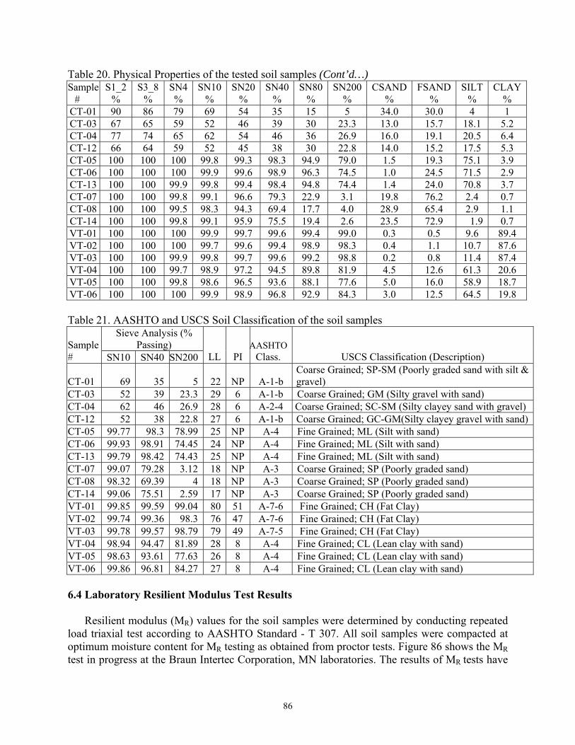
86

Table 20. Physical Properties of the tested soil samples (Cont’d…) Sample S1_2 S3_8 SN4 SN10 SN20 SN40 SN80 SN200 CSAND FSAND SILT CLAY # % % % % % % % % % % % % CT-01 90 86 79 69 54 35 15 5 34.0 30.0 4 1CT-03 67 65 59 52 46 39 30 23.3 13.0 15.7 18.1 5.2CT-04 77 74 65 62 54 46 36 26.9 16.0 19.1 20.5 6.4CT-12 66 64 59 52 45 38 30 22.8 14.0 15.2 17.5 5.3CT-05 100 100 100 99.8 99.3 98.3 94.9 79.0 1.5 19.3 75.1 3.9CT-06 100 100 100 99.9 99.6 98.9 96.3 74.5 1.0 24.5 71.5 2.9CT-13 100 100 99.9 99.8 99.4 98.4 94.8 74.4 1.4 24.0 70.8 3.7CT-07 100 100 99.8 99.1 96.6 79.3 22.9 3.1 19.8 76.2 2.4 0.7CT-08 100 100 99.5 98.3 94.3 69.4 17.7 4.0 28.9 65.4 2.9 1.1CT-14 100 100 99.8 99.1 95.9 75.5 19.4 2.6 23.5 72.9 1.9 0.7VT-01 100 100 100 99.9 99.7 99.6 99.4 99.0 0.3 0.5 9.6 89.4VT-02 100 100 100 99.7 99.6 99.4 98.9 98.3 0.4 1.1 10.7 87.6VT-03 100 100 99.9 99.8 99.7 99.6 99.2 98.8 0.2 0.8 11.4 87.4VT-04 100 100 99.7 98.9 97.2 94.5 89.8 81.9 4.5 12.6 61.3 20.6VT-05 100 100 99.8 98.6 96.5 93.6 88.1 77.6 5.0 16.0 58.9 18.7VT-06 100 100 100 99.9 98.9 96.8 92.9 84.3 3.0 12.5 64.5 19.8

Table 21. AASHTO and USCS Soil Classification of the soil samples

Sieve Analysis (% Passing) Sample

# SN10 SN40 SN200 LL PI AASHTO

Class. USCS Classification (Description)

CT-01 69 35 5 22 NP A-1-b Coarse Grained; SP-SM (Poorly graded sand with silt & gravel)

CT-03 52 39 23.3 29 6 A-1-b Coarse Grained; GM (Silty gravel with sand) CT-04 62 46 26.9 28 6 A-2-4 Coarse Grained; SC-SM (Silty clayey sand with gravel) CT-12 52 38 22.8 27 6 A-1-b Coarse Grained; GC-GM(Silty clayey gravel with sand)CT-05 99.77 98.3 78.99 25 NP A-4 Fine Grained; ML (Silt with sand) CT-06 99.93 98.91 74.45 24 NP A-4 Fine Grained; ML (Silt with sand) CT-13 99.79 98.42 74.43 25 NP A-4 Fine Grained; ML (Silt with sand) CT-07 99.07 79.28 3.12 18 NP A-3 Coarse Grained; SP (Poorly graded sand) CT-08 98.32 69.39 4 18 NP A-3 Coarse Grained; SP (Poorly graded sand) CT-14 99.06 75.51 2.59 17 NP A-3 Coarse Grained; SP (Poorly graded sand) VT-01 99.85 99.59 99.04 80 51 A-7-6 Fine Grained; CH (Fat Clay) VT-02 99.74 99.36 98.3 76 47 A-7-6 Fine Grained; CH (Fat Clay) VT-03 99.78 99.57 98.79 79 49 A-7-5 Fine Grained; CH (Fat Clay) VT-04 98.94 94.47 81.89 28 8 A-4 Fine Grained; CL (Lean clay with sand) VT-05 98.63 93.61 77.63 26 8 A-4 Fine Grained; CL (Lean clay with sand) VT-06 99.86 96.81 84.27 27 8 A-4 Fine Grained; CL (Lean clay with sand) 6.4 Laboratory Resilient Modulus Test Results

Resilient modulus (MR) values for the soil samples were determined by conducting repeated load triaxial test according to AASHTO Standard - T 307. All soil samples were compacted at optimum moisture content for MR testing as obtained from proctor tests. Figure 86 shows the MR test in progress at the Braun Intertec Corporation, MN laboratories. The results of MR tests have

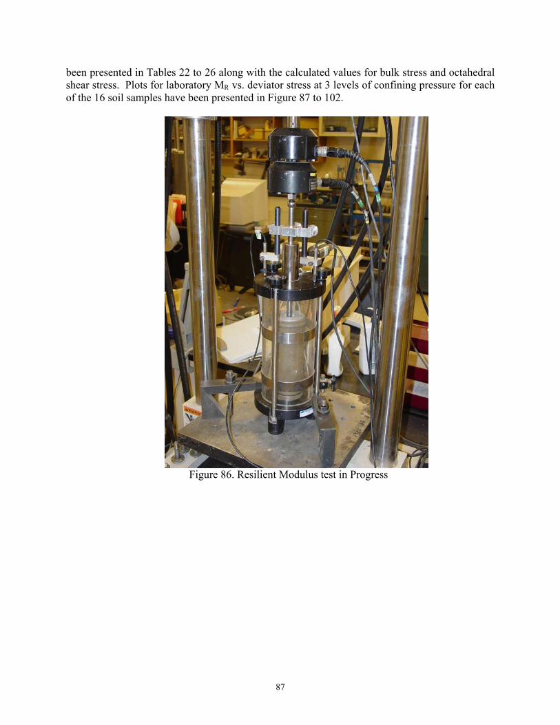
87

been presented in Tables 22 to 26 along with the calculated values for bulk stress and octahedral shear stress. Plots for laboratory MR vs. deviator stress at 3 levels of confining pressure for each of the 16 soil samples have been presented in Figure 87 to 102.

Figure 86. Resilient Modulus test in Progress

88

Table 22. Laboratory MR test results for A-1-b (Coarse Grained) soils

Sample #

Confining Pressure, σ3

kPa

Deviator/Applied Cyclic Stress, σd

kPa Bulk Stress, θ

kPa

Octahderal Shear Stress, τoct

kPa Lab MR

MPa CT-01 41.4 12.4 136.543 5.844 90 CT-01 41.3 24.9 148.9107 11.73 95 CT-01 41.4 37.3 161.3396 17.57 96 CT-01 41.4 49.6 173.7291 23.397 97 CT-01 41.3 62.0 185.9857 29.209 98 CT-01 27.6 12.2 94.95913 5.76 66 CT-01 27.6 24.5 107.3068 11.536 67 CT-01 27.6 37.1 119.7979 17.467 71 CT-01 27.6 49.6 132.2365 23.37 76 CT-01 27.6 61.9 144.558 29.165 78 CT-01 13.8 12.2 53.54541 5.743 45 CT-01 13.8 24.4 65.77769 11.487 47 CT-01 13.8 36.8 78.25656 17.369 51

CT-03 41.4 12.6 136.7239 5.936 112 CT-03 41.4 25.3 149.3539 11.919 111 CT-03 41.4 37.7 161.7791 17.777 103 CT-03 41.3 49.9 173.9062 23.503 98 CT-03 41.4 62.4 186.4499 29.406 95 CT-03 27.6 12.6 95.37337 5.95 96 CT-03 27.6 25.2 107.8967 11.857 93 CT-03 27.6 37.7 120.3987 17.755 89 CT-03 27.6 49.9 132.5941 23.508 86 CT-03 27.6 62.3 145.0699 29.392 85 CT-03 13.8 12.6 53.91231 5.923 68 CT-03 13.8 25.0 66.36555 11.806 67 CT-03 13.8 37.3 78.65348 17.59 67 CT-03 13.8 49.7 91.0308 23.434 68 CT-03 13.8 62.2 103.6077 29.309 69

CT-12 41.4 12.6 136.7673 5.929 104 CT-12 41.4 25.1 149.2869 11.853 99 CT-12 41.4 37.6 161.6882 17.712 91 CT-12 41.4 49.8 173.8793 23.479 86 CT-12 41.3 62.2 186.2572 29.329 84 CT-12 27.6 12.6 95.25718 5.925 90 CT-12 27.6 25.0 107.6961 11.794 83 CT-12 27.6 37.3 120.0017 17.593 77 CT-12 27.6 49.7 132.3444 23.413 74 CT-12 27.6 62.2 145.0164 29.334 74 CT-12 13.8 12.5 53.75588 5.888 70 CT-12 13.8 24.9 66.23222 11.728 64 CT-12 13.8 37.1 78.47615 17.503 61 CT-12 13.8 49.5 90.89508 23.358 60 CT-12 13.8 62.0 103.3961 29.249 61

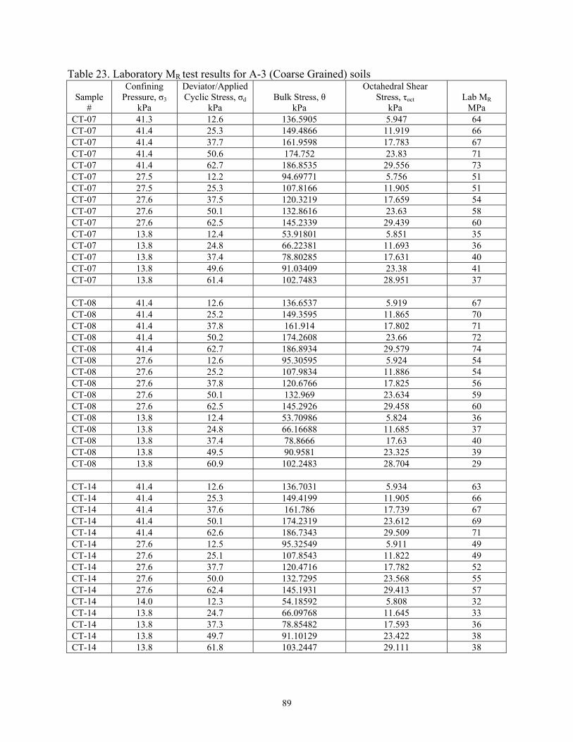
89

Table 23. Laboratory MR test results for A-3 (Coarse Grained) soils

Sample #


kPa


kPa Bulk Stress, θ

kPa

Octahedral Shear Stress, τoct

kPa Lab MR

MPa CT-07 41.3 12.6 136.5905 5.947 64 CT-07 41.4 25.3 149.4866 11.919 66 CT-07 41.4 37.7 161.9598 17.783 67 CT-07 41.4 50.6 174.752 23.83 71 CT-07 41.4 62.7 186.8535 29.556 73 CT-07 27.5 12.2 94.69771 5.756 51 CT-07 27.5 25.3 107.8166 11.905 51 CT-07 27.6 37.5 120.3219 17.659 54 CT-07 27.6 50.1 132.8616 23.63 58 CT-07 27.6 62.5 145.2339 29.439 60 CT-07 13.8 12.4 53.91801 5.851 35 CT-07 13.8 24.8 66.22381 11.693 36 CT-07 13.8 37.4 78.80285 17.631 40 CT-07 13.8 49.6 91.03409 23.38 41 CT-07 13.8 61.4 102.7483 28.951 37 CT-08 41.4 12.6 136.6537 5.919 67 CT-08 41.4 25.2 149.3595 11.865 70 CT-08 41.4 37.8 161.914 17.802 71 CT-08 41.4 50.2 174.2608 23.66 72 CT-08 41.4 62.7 186.8934 29.579 74 CT-08 27.6 12.6 95.30595 5.924 54 CT-08 27.6 25.2 107.9834 11.886 54 CT-08 27.6 37.8 120.6766 17.825 56 CT-08 27.6 50.1 132.969 23.634 59 CT-08 27.6 62.5 145.2926 29.458 60 CT-08 13.8 12.4 53.70986 5.824 36 CT-08 13.8 24.8 66.16688 11.685 37 CT-08 13.8 37.4 78.8666 17.63 40 CT-08 13.8 49.5 90.9581 23.325 39 CT-08 13.8 60.9 102.2483 28.704 29 CT-14 41.4 12.6 136.7031 5.934 63 CT-14 41.4 25.3 149.4199 11.905 66 CT-14 41.4 37.6 161.786 17.739 67 CT-14 41.4 50.1 174.2319 23.612 69 CT-14 41.4 62.6 186.7343 29.509 71 CT-14 27.6 12.5 95.32549 5.911 49 CT-14 27.6 25.1 107.8543 11.822 49 CT-14 27.6 37.7 120.4716 17.782 52 CT-14 27.6 50.0 132.7295 23.568 55 CT-14 27.6 62.4 145.1931 29.413 57 CT-14 14.0 12.3 54.18592 5.808 32 CT-14 13.8 24.7 66.09768 11.645 33 CT-14 13.8 37.3 78.85482 17.593 36 CT-14 13.8 49.7 91.10129 23.422 38 CT-14 13.8 61.8 103.2447 29.111 38

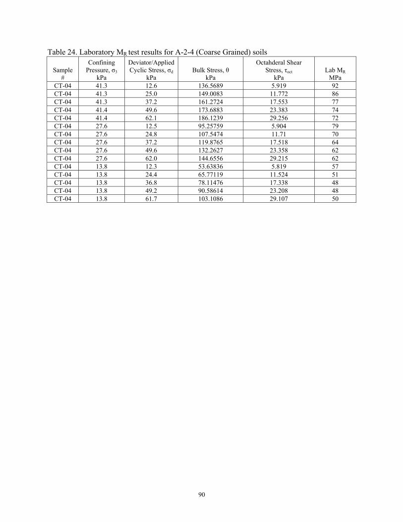
90

Table 24. Laboratory MR test results for A-2-4 (Coarse Grained) soils

Sample #


kPa


kPa Bulk Stress, θ

kPa


kPa Lab MR

MPa CT-04 41.3 12.6 136.5689 5.919 92 CT-04 41.3 25.0 149.0083 11.772 86 CT-04 41.3 37.2 161.2724 17.553 77 CT-04 41.4 49.6 173.6883 23.383 74 CT-04 41.4 62.1 186.1239 29.256 72 CT-04 27.6 12.5 95.25759 5.904 79 CT-04 27.6 24.8 107.5474 11.71 70 CT-04 27.6 37.2 119.8765 17.518 64 CT-04 27.6 49.6 132.2627 23.358 62 CT-04 27.6 62.0 144.6556 29.215 62 CT-04 13.8 12.3 53.63836 5.819 57 CT-04 13.8 24.4 65.77119 11.524 51 CT-04 13.8 36.8 78.11476 17.338 48 CT-04 13.8 49.2 90.58614 23.208 48 CT-04 13.8 61.7 103.1086 29.107 50

91

Table 25. Laboratory MR test results for A-4 (Fine Grained) soils

Sample #


kPa


kPa Bulk Stress, θ

kPa


kPa Lab MR

MPa CT-05 41.4 12.6 136.67935 5.937 68 CT-05 41.4 25.3 149.36222 11.912 63 CT-05 41.4 37.7 161.78323 17.751 60 CT-05 41.4 50.1 174.2208 23.623 59 CT-05 41.4 62.6 186.7269 29.532 59 CT-05 27.6 12.5 95.343661 5.914 58 CT-05 27.6 24.8 107.61989 11.707 50 CT-05 27.6 37.3 120.02447 17.563 47 CT-05 27.6 50.0 132.76306 23.562 46 CT-05 27.6 62.8 145.56705 29.613 47 CT-05 13.8 12.3 53.745617 5.805 38 CT-05 13.8 24.5 65.938742 11.541 33 CT-05 13.8 36.9 78.34112 17.391 32 CT-05 13.8 49.5 90.892613 23.325 33 CT-05 13.8 62.1 103.4879 29.286 36 CT-06 41.4 12.6 136.62637 5.924 69 CT-06 41.3 25.2 149.25254 11.881 63 CT-06 41.4 37.6 161.6839 17.712 60 CT-06 41.4 49.9 174.00056 23.532 59 CT-06 41.4 62.5 186.52138 29.446 59 CT-06 27.6 12.5 95.300899 5.909 59 CT-06 27.6 24.9 107.61899 11.719 52 CT-06 27.6 37.4 120.15131 17.623 48 CT-06 27.6 50.0 132.75111 23.561 48 CT-06 27.6 62.5 145.20844 29.441 49 CT-06 13.8 12.3 53.610368 5.787 40 CT-06 13.8 24.5 65.808666 11.547 35 CT-06 13.8 37.0 78.265212 17.434 34 CT-06 13.8 49.5 90.88181 23.347 36 CT-06 13.8 62.3 103.6967 29.39 38 CT-13 41.4 12.5 136.57578 5.895 56 CT-13 41.4 25.2 149.29333 11.897 53 CT-13 41.4 37.6 161.80361 17.745 52 CT-13 41.4 49.9 174.07 23.537 53 CT-13 41.4 62.5 186.5935 29.449 55 CT-13 27.6 12.4 95.119469 5.846 47 CT-13 27.6 24.6 107.25223 11.577 42 CT-13 27.6 37.2 119.89295 17.538 40 CT-13 27.6 49.7 132.46311 23.425 41 CT-13 27.6 62.4 145.13708 29.405 44 CT-13 13.8 12.3 53.582594 5.775 33 CT-13 13.8 24.5 65.79649 11.531 29 CT-13 13.8 36.9 78.169296 17.376 29 CT-13 13.8 49.5 90.882563 23.339 31 CT-13 13.8 62.3 103.71662 29.372 34

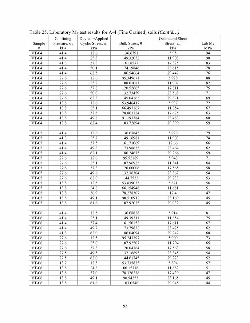
92

Table 25. Laboratory MR test results for A-4 (Fine Grained) soils (Cont’d…)

Sample #


kPa


kPa Bulk Stress, θ

kPa


kPa Lab MR

MPa VT-04 41.4 12.6 136.6791 5.95 94 VT-04 41.4 25.3 149.32052 11.908 90 VT-04 41.3 37.8 161.8577 17.825 83 VT-04 41.4 50.1 174.19846 23.615 78 VT-04 41.4 62.5 186.54664 29.447 76 VT-04 27.6 12.6 95.349671 5.928 88 VT-04 27.6 25.2 108.01081 11.902 82 VT-04 27.6 37.8 120.52665 17.811 75 VT-04 27.6 50.0 132.73459 23.568 71 VT-04 27.6 62.3 145.04165 29.371 69 VT-04 13.8 12.6 53.946417 5.937 72 VT-04 13.8 25.1 66.497167 11.854 67 VT-04 13.8 37.5 78.863724 17.675 63 VT-04 13.8 49.8 91.193384 23.483 60 VT-04 13.8 62.4 103.72694 29.399 59 VT-05 41.4 12.6 136.67845 5.929 79 VT-05 41.3 25.2 149.16981 11.903 74 VT-05 41.4 37.5 161.71069 17.66 66 VT-05 41.4 49.8 173.98635 23.464 62 VT-05 41.4 62.1 186.24675 29.266 59 VT-05 27.6 12.6 95.52189 5.943 71 VT-05 27.6 25.1 107.96925 11.841 64 VT-05 27.6 37.3 120.00006 17.565 58 VT-05 27.6 49.6 132.36304 23.367 54 VT-05 27.6 62.0 144.7532 29.233 53 VT-05 13.8 12.5 53.839035 5.871 56 VT-05 13.8 24.8 66.154948 11.681 51 VT-05 13.8 36.9 78.278307 17.4 47 VT-05 13.8 49.1 90.510912 23.169 45 VT-05 13.8 61.6 102.92035 29.032 45 VT-06 41.4 12.5 136.68828 5.914 81 VT-06 41.4 25.1 149.39311 11.854 75 VT-06 41.4 37.4 161.50152 17.611 67 VT-06 41.4 49.7 173.79832 23.425 62 VT-06 41.3 62.0 186.04094 29.247 60 VT-06 27.6 12.5 95.243397 5.909 73 VT-06 27.6 25.0 107.92507 11.794 65 VT-06 27.6 37.3 120.04764 17.563 58 VT-06 27.5 49.5 132.16895 23.345 54 VT-06 27.5 62.0 144.61745 29.223 52 VT-06 13.7 12.5 53.735835 5.894 57 VT-06 13.8 24.8 66.15318 11.682 51 VT-06 13.8 37.0 78.326238 17.439 47 VT-06 13.8 49.1 90.54253 23.165 45 VT-06 13.8 61.6 103.0546 29.045 44

93

Table 26. Laboratory MR test results for A-7-6 (Fine Grained) soils

Sample #


kPa


kPa Bulk Stress, θ

kPa


kPa Lab MR

MPa VT-01 41.3 12.5 136.5551 5.897 70 VT-01 41.4 25.0 149.0687 11.768 69 VT-01 41.4 37.3 161.4119 17.594 65 VT-01 41.4 49.5 173.5723 23.337 61 VT-01 41.3 61.8 185.8015 29.111 58 VT-01 27.6 12.5 95.1744 5.876 65 VT-01 27.6 24.9 107.6087 11.747 64 VT-01 27.6 37.2 119.8995 17.544 61 VT-01 27.6 49.4 132.0691 23.291 58 VT-01 27.6 61.8 144.5699 29.112 56 VT-01 13.8 12.4 53.7749 5.841 50 VT-01 13.8 24.7 66.0944 11.662 53 VT-01 13.8 37.1 78.4231 17.489 54 VT-01 13.8 49.3 90.6679 23.252 53 VT-01 13.8 61.6 102.9336 29.05 52

VT-02 41.4 12.5 136.5949 5.898 61 VT-02 41.4 25.0 149.0234 11.77 59 VT-02 41.3 37.1 161.1261 17.489 55 VT-02 41.4 49.3 173.3716 23.227 52 VT-02 41.4 61.4 185.4293 28.923 48 VT-02 27.5 12.5 95.1050 5.883 57 VT-02 27.6 24.9 107.7341 11.747 56 VT-02 27.6 37.1 119.8738 17.473 54 VT-02 27.6 49.1 131.8940 23.163 51 VT-02 27.6 61.4 144.2530 28.961 49 VT-02 13.8 12.3 53.8014 5.815 44 VT-02 13.8 24.6 66.0137 11.594 45 VT-02 13.8 36.8 78.2077 17.36 44 VT-02 13.8 48.9 90.3551 23.052 44 VT-02 13.8 61.2 102.5254 28.834 43

VT-03 41.4 12.6 136.6212 5.917 66 VT-03 41.3 24.9 148.9180 11.728 64 VT-03 41.3 37.1 161.1451 17.504 61 VT-03 41.3 49.3 173.3510 23.253 57 VT-03 41.3 61.6 185.6909 29.058 55 VT-03 27.6 12.5 95.2237 5.878 61 VT-03 27.5 24.9 107.5035 11.721 60 VT-03 27.6 37.1 119.8887 17.494 57 VT-03 27.6 49.3 132.2173 23.241 54 VT-03 27.6 61.6 144.3945 29.037 52 VT-03 13.8 12.4 53.8377 5.865 50 VT-03 13.8 24.7 66.0289 11.64 51 VT-03 13.8 36.9 78.3263 17.414 50 VT-03 13.8 49.1 90.4940 23.164 49 VT-03 13.8 61.4 102.7167 28.932 48

94

CT- 01

0

20,000

40,000

60,000

80,000

100,000

120,000

0.0 10.0 20.0 30.0 40.0 50.0 60.0 70.0Deviator Stress (kPa)

Labo

rato

ry M

R (k

Pa)

Confining Pressure 41.4 kPaConfining Pressure 27.6 kPaConfining Pressure 13.8 kPa

Figure 87. Laboratory Resilient Modulus (MR) vs. Deviator stress for CT-01

CT - 03

0

20,000

40,000

60,000

80,000

100,000

120,000


Labo

rato

ry M

R (k

Pa)

Confining Pressure 41.4 kPa




95

CT - 04

0

20,000

40,000

60,000

80,000

100,000


Labo

rato

ry M

R (k

Pa)





CT - 05

0

20,000

40,000

60,000

80,000


Labo

rato

ry M

R (k

Pa)





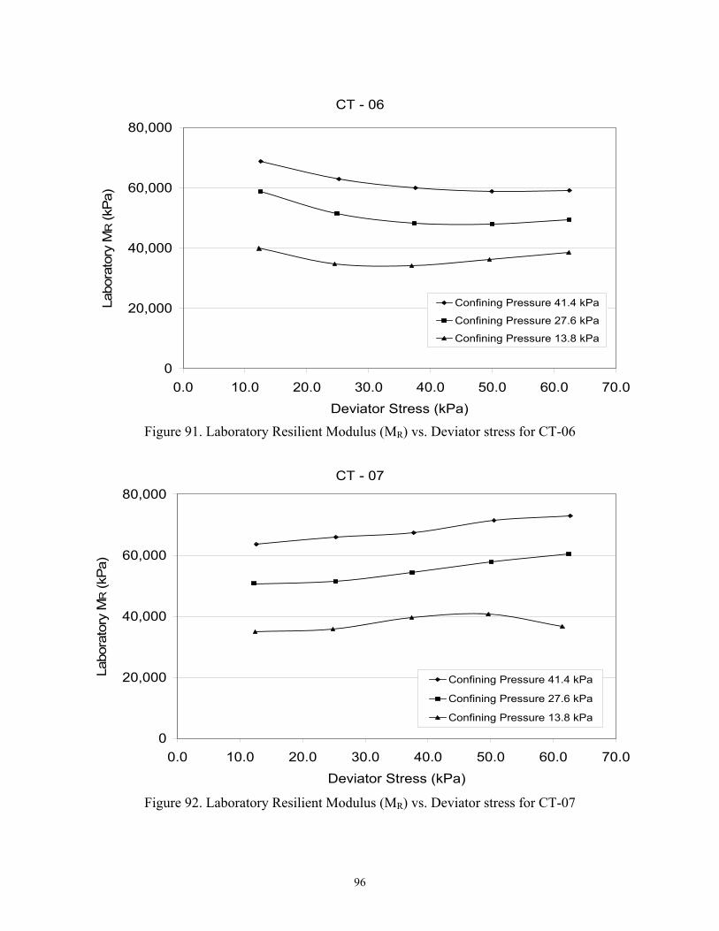
96

CT - 06

0

20,000

40,000

60,000

80,000


Labo

rato

ry M

R (k

Pa)





CT - 07

0

20,000

40,000

60,000

80,000


Labo

rato

ry M

R (k

Pa)





97

CT - 08

0

20,000

40,000

60,000

80,000


Labo

rato

ry M

R (k

Pa)





CT - 12

0

20,000

40,000

60,000

80,000

100,000

120,000


Labo

rato

ry M

R (k

Pa)





98

CT - 13

0

20,000

40,000

60,000


Labo

rato

ry M

R (k

Pa)





CT- 14

0

20,000

40,000

60,000

80,000


Labo

rato

ry M

R (k

Pa)





99

VT - 01

0

20,000

40,000

60,000

80,000


Labo

rato

ry M

R (k

Pa)




Figure 97. Laboratory Resilient Modulus (MR) vs. Deviator stress for VT-01

VT - 02

0

20,000

40,000

60,000

80,000


Labo

rato

ry M

R (k

Pa)





100

VT - 03

0

20,000

40,000

60,000

80,000


Labo

rato

ry M

R (k

Pa)





VT - 04

0

20,000

40,000

60,000

80,000

100,000


Labo

rato

ry M

R (k

Pa)





101

VT - 05

0

20,000

40,000

60,000

80,000

100,000


Labo

rato

ry M

R (k

Pa)





VT - 06

0

20,000

40,000

60,000

80,000

100,000


Labo

rato

ry M

R (k

Pa)





102

6.5 Verification of Prediction Models Developed for AASHTO Soil Types

In order to verify the prediction models developed in Section 4.3 for the different AASHTO soil types, the values of the soil properties mentioned in the Table 20 were substituted in the corresponding k coefficients equations for each soil type. For each soil sample, k coefficients were determined for 2 set of prediction models (see Section 4.3.3), the first set of models had been developed using all the reconstituted samples and the second set of models had been developed using only those soil samples that were compacted at optimum moisture content which will be referred as MODEL1 and MODEL2 respectively hereafter.

The value of k coefficients obtained from the MODEL1 and MODEL2 for each soil

specimen has been presented in Table 27. The values of k coefficients calculated by regression of laboratory MR values and corresponding stresses using the generalized constitutive model as described in Section 4.3.2 has also been presented in Table 27.

Table 27. Comparison of values k coefficients obtained from regression of each sample and those obtained from the prediction models developed for different AASHTO soil types

Sample # k coefficients evaluated from the prediction models

k coefficients from regression of lab test values MODEL1* MODEL2**

log k1 k2 k3 log k1 k2 k3 log k1 k2 k3 CT-01 -0.29497 0.82099 -0.11852 -0.16032 0.68906 -0.28038 -0.25161 0.72315 -0.19518CT-03 -0.28467 0.57236 -0.22403 -0.22894 0.54259 -0.15274 -1.61057 1.31005 -0.33468CT-12 -0.35937 0.50461 -0.26561 -0.22943 0.44594 -0.1214 -2.1829 1.47774 -0.32714

CT-04 -0.48107 0.61563 -0.31157 -0.60032 0.43058 -0.41346 -0.7757 1.15788 -0.51261

CT-05 -0.6323 0.78118 -0.3186 -0.71994 0.60058 -0.36046 -0.5787 0.45017 -0.30857CT-06 -0.58682 0.70951 -0.28494 -0.72392 0.61151 -0.3555 -0.56706 0.47583 -0.30164CT-13 -0.61851 0.74289 -0.23706 -0.72242 0.61551 -0.36015 -0.58046 0.47006 -0.31023

CT-07 -0.43988 0.78383 -0.13487 -0.4652 0.67678 -0.15122 -0.37173 0.67091 -0.15118CT-08 -0.50591 0.85509 -0.21813 -0.41169 0.62246 -0.15101 -0.32249 0.72017 -0.16151CT-14 -0.46548 0.8488 -0.14186 -0.43579 0.6458 -0.1455 -0.34911 0.72466 -0.15802

VT-01 -0.36846 0.2883 -0.14468 -0.90371 -0.26108 -0.43303 -0.93935 -0.24357 -0.57419VT-02 -0.46293 0.30817 -0.1767 -0.84032 -0.19491 -0.40655 -0.88908 -0.22747 -0.54705VT-03 -0.40204 0.26889 -0.15416 -0.88128 -0.24734 -0.4328 -0.89928 -0.22257 -0.55156

VT-04 -0.34964 0.3558 -0.24126 -0.39967 0.34242 -0.32312 -0.35339 0.3688 -0.2966VT-05 -0.51023 0.43552 -0.30142 -0.61611 0.41975 -0.40437 -0.62021 0.40431 -0.41173VT-06 -0.52643 0.45383 -0.32336 -0.57854 0.39203 -0.39273 -0.57341 0.3673 -0.38268

*MODEL1 – Models developed using all the reconstituted samples **MODEL2 - Models developed using only those soil samples that were compacted at optimum moisture content

103

After evaluating the value of the k coefficients from the prediction models for each soil sample, the value of k coefficients were substituted in the generalized constitutive model

equation, ( ) ⎟⎟⎠

⎞⎜⎜⎝

⎛+⎟⎟

⎠

⎞⎜⎜⎝

⎛+=

a

oct

aaR P

kP

kPkMτθ loglogloglog 321 . The bulk stress and

octahedral shear stress values were calculated for each combination of corresponding confining pressure and axial cyclic stress applied during laboratory testing resulting in 15 levels of stresses for each soil sample. The substitution of k coefficient for each soil specimen and these 15 values of bulk and octahedral shear stress give 15 values of MR for each soil specimen at different levels of stresses. This process was performed for both MODEL1 and MODEL2.

6.5.1 Verification of Prediction Model for A-1-b Soil

The laboratory MR values and MR values calculated from the prediction models for the A-1-b soil CT-03 and CT12 has been presented in tabular and graphical forms in Table 28 and Figure 103. CT-01 has not been included here in spite of being an A-1-b soil since it is a Material Type 1 soil but the models developed herein this report were based on Material Type 2 soils only. AASHTO - T 307 defines the Material Type 1 as soils which meet the criteria of less than 70% passing the No. 10 sieve and less than 20% passing the No. 200 sieve, and which have a plasticity index of 10 or less. Material Type 2 are the soils not meeting the criteria given for Material Type 1.

Predicted MR values calculated from MODEL1 only has been presented in Tables 28 and

Figure 103. The MR values predicted from MODEL2 did not quite match the laboratory MR values since the values of soil properties parameters S1_HALF and FSAND were out of the soil properties range from which MODEL2 was developed, hence requiring extrapolation which results in incredible results.

Table 28. Comparison of Laboratory and Predicted MR values for A-1-b soils

Predicted MR Lab MR MODEL1 Sample

# MPa MPa CT-03 112 108.54 CT-03 111 102.37 CT-03 103 100.57 CT-03 98 100.23 CT-03 95 100.59 CT-03 96 89.24 CT-03 93 85.88 CT-03 89 85.69 CT-03 86 86.51 CT-03 85 87.79 CT-03 68 65.53 CT-03 67 66.02 CT-03 67 68.12 CT-03 68 70.58 CT-03 69 73.17

CT-12 104 96.39

104

Table 28. Comparison of Laboratory and Predicted MR values for A-1-b soils (Cont’d…) Predicted MR

Lab MR MODEL1 Sample # MPa MPa

CT-12 99 92.15 CT-12 91 90.94 CT-12 86 90.78 CT-12 84 91.11 CT-12 90 82.04 CT-12 83 79.71 CT-12 77 79.68 CT-12 74 80.4 CT-12 74 81.49 CT-12 70 63.61 CT-12 64 64.22 CT-12 61 65.98 CT-12 60 68.02 CT-12 61 70.1

0

20

40

60

80

100

120

0 20 40 60 80 100 120Laboratory MR (MPa)

Pred

icte

d M

R (M

Pa)

Figure 103. Predicted MR from MODEL1 vs. Laboratory MR for A-1-b soil samples CT-03 and

CT-12

Evaluation of the MR values shows that for MODEL1 90% of predicted MR values were within ±10% of the laboratory MR values and 100% of predicted MR values were within ±20% of the laboratory MR values.

6.5.2 Verification of Prediction Model for A-3 Soil

The laboratory MR values and MR values calculated from the prediction models (MODEL1 and MODEL2) for the A-3 soils CT-07, CT-08, and CT-14 have been presented in tabular and graphical forms in Table 29 and Figure 104 and 105.

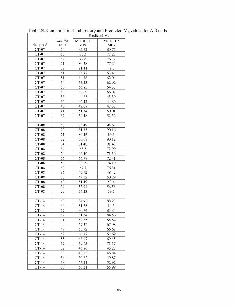
105

Table 29. Comparison of Laboratory and Predicted MR values for A-3 soils Predicted MR

Lab MR MODEL1 MODEL2Sample # MPa MPa MPa

CT-07 64 83.92 80.75 CT-07 66 80.3 77.23 CT-07 67 79.8 76.72 CT-07 71 80.38 77.24 CT-07 73 81.41 78.2 CT-07 51 65.82 63.47 CT-07 51 64.38 62.04 CT-07 54 65.33 62.92 CT-07 58 66.85 64.35 CT-07 60 68.69 66.07 CT-07 35 44.85 43.39 CT-07 36 46.42 44.86 CT-07 40 49.07 47.37 CT-07 41 51.84 50.01 CT-07 37 54.48 52.52



106

0

20

40

60

80

100


Pre

dict

ed M

R (M

Pa)

Figure 104. Predicted MR from MODEL1 vs. Laboratory MR for A-3 soil samples CT-07, CT-08, CT-14

A-3 (MODEL2)

0

20

40

60

80

100


Pre

dict

ed M

R (M

Pa)

Figure 105. Predicted MR from MODEL2 vs. Laboratory MR for A-3 soil samples CT-07, CT-08, CT-14

Evaluation of the MR values show 68.89% of predicted MR were within ± 10% of the

laboratory MR values and 97.78% of predicted MR were within ± 20% of the laboratory MR values for MODEL1. Similarly incase of MODEL2, 6.67% of predicted MR values were within

107

±10% of the laboratory MR and 17.78% of predicted MR values were within ± 20% of the laboratory MR values.

6.5.3 Verification of Prediction Model for A-2-4 Soil

The laboratory MR values and MR values calculated from the prediction models (MODEL1 and MODEL2) for the A-2.4 soil CT-04 has been presented in tabular and graphical forms in Table 30 and Figure 106 and 107.

Table 30. Comparison of Laboratory and Predicted MR values for A-2-4 soils

Predicted MR Lab MR MODEL1 MODEL2 Sample

# MPa MPa MPa CT-04 92 93.58 102.9 CT-04 86 73.12 80.01 CT-04 77 64.13 71.45 CT-04 74 58.81 67.21 CT-04 72 55.23 64.92 CT-04 79 80.22 67.89 CT-04 70 63.68 55 CT-04 64 56.49 50.73 CT-04 62 52.32 49.05 CT-04 62 49.58 48.52 CT-04 57 63.02 35.18 CT-04 51 51.87 31.38 CT-04 48 47.18 31.06 CT-04 48 44.57 31.75 CT-04 50 42.92 32.85

0

20

40

60

80

100

120


Pre

dict

ed M

R (M

Pa)

Figure 106. Predicted MR from MODEL1 vs. Laboratory MR for A-2-4 soil sample CT-04

108

0

20

40

60

80

100

120


Pre

dict

ed M

R (M

Pa)

Figure 107. Predicted MR from MODEL2 vs. Laboratory MR for A-2-4 soil samples CT-04

Evaluation of the MR values show that 40.0% of predicted MR values were within ± 10% of

the laboratory MR values and 86.67% of predicted MR values were within ± 20% of the laboratory MR values for MODEL1. Similarly incase of MODEL2, 20.0% of predicted MR values were within ±10% of the laboratory MR values and 40.0% of predicted MR values were within ± 20% of the laboratory MR values. 6.5.4 Verification of Prediction Model for A-4 Soil

The laboratory MR values and MR values calculated from the prediction models (MODEL1 and MODEL2) for the A-4 soil CT-05, CT-06, CT-13, VT04- VT-05, and VT-06 have been presented in tabular and graphical forms in Table 31 and Figure 108 and 109.

0

20

40

60

80

100

120


Pre

dict

ed M

R (M

Pa)

Figure 108. Predicted MR from MODEL1 vs. Laboratory MR for A-4 soil sample CT-05, CT-06,

CT-13, VT-04, VT-05, and VT-06

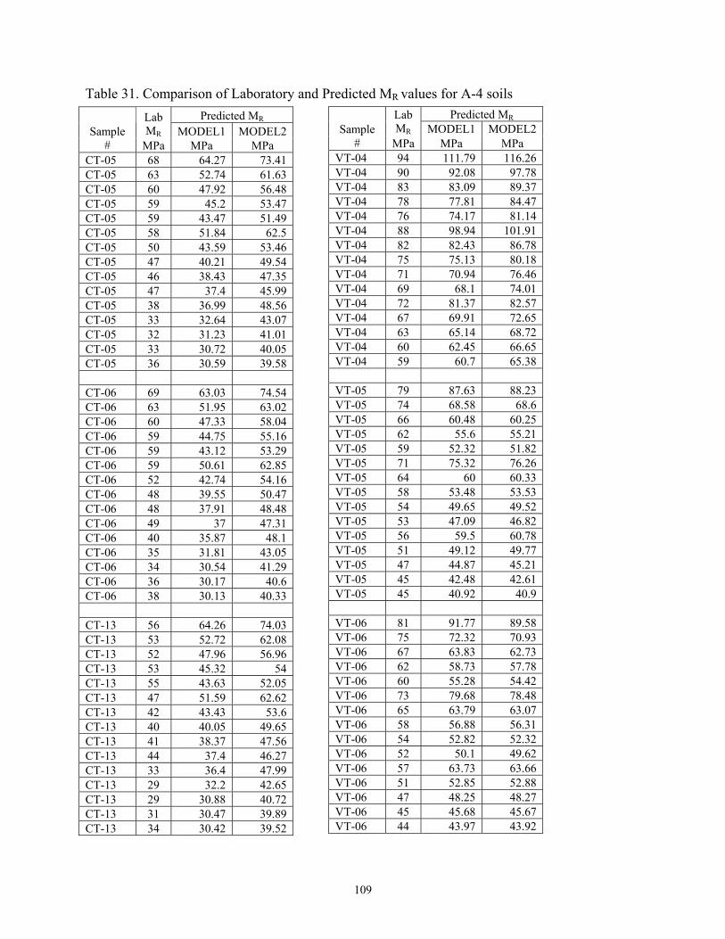
109

Table 31. Comparison of Laboratory and Predicted MR values for A-4 soils


# MPa MPa MPa CT-05 68 64.27 73.41 CT-05 63 52.74 61.63 CT-05 60 47.92 56.48 CT-05 59 45.2 53.47 CT-05 59 43.47 51.49 CT-05 58 51.84 62.5 CT-05 50 43.59 53.46 CT-05 47 40.21 49.54 CT-05 46 38.43 47.35 CT-05 47 37.4 45.99 CT-05 38 36.99 48.56 CT-05 33 32.64 43.07 CT-05 32 31.23 41.01 CT-05 33 30.72 40.05 CT-05 36 30.59 39.58 CT-06 69 63.03 74.54 CT-06 63 51.95 63.02 CT-06 60 47.33 58.04 CT-06 59 44.75 55.16 CT-06 59 43.12 53.29 CT-06 59 50.61 62.85 CT-06 52 42.74 54.16 CT-06 48 39.55 50.47 CT-06 48 37.91 48.48 CT-06 49 37 47.31 CT-06 40 35.87 48.1 CT-06 35 31.81 43.05 CT-06 34 30.54 41.29 CT-06 36 30.17 40.6 CT-06 38 30.13 40.33 CT-13 56 64.26 74.03 CT-13 53 52.72 62.08 CT-13 52 47.96 56.96 CT-13 53 45.32 54 CT-13 55 43.63 52.05 CT-13 47 51.59 62.62 CT-13 42 43.43 53.6 CT-13 40 40.05 49.65 CT-13 41 38.37 47.56 CT-13 44 37.4 46.27 CT-13 33 36.4 47.99 CT-13 29 32.2 42.65 CT-13 29 30.88 40.72 CT-13 31 30.47 39.89 CT-13 34 30.42 39.52


# MPa MPa MPa VT-04 94 111.79 116.26 VT-04 90 92.08 97.78 VT-04 83 83.09 89.37 VT-04 78 77.81 84.47 VT-04 76 74.17 81.14 VT-04 88 98.94 101.91 VT-04 82 82.43 86.78 VT-04 75 75.13 80.18 VT-04 71 70.94 76.46 VT-04 69 68.1 74.01 VT-04 72 81.37 82.57 VT-04 67 69.91 72.65 VT-04 63 65.14 68.72 VT-04 60 62.45 66.65 VT-04 59 60.7 65.38 VT-05 79 87.63 88.23 VT-05 74 68.58 68.6 VT-05 66 60.48 60.25 VT-05 62 55.6 55.21 VT-05 59 52.32 51.82 VT-05 71 75.32 76.26 VT-05 64 60 60.33 VT-05 58 53.48 53.53 VT-05 54 49.65 49.52 VT-05 53 47.09 46.82 VT-05 56 59.5 60.78 VT-05 51 49.12 49.77 VT-05 47 44.87 45.21 VT-05 45 42.48 42.61 VT-05 45 40.92 40.9 VT-06 81 91.77 89.58 VT-06 75 72.32 70.93 VT-06 67 63.83 62.73 VT-06 62 58.73 57.78 VT-06 60 55.28 54.42 VT-06 73 79.68 78.48 VT-06 65 63.79 63.07 VT-06 58 56.88 56.31 VT-06 54 52.82 52.32 VT-06 52 50.1 49.62 VT-06 57 63.73 63.66 VT-06 51 52.85 52.88 VT-06 47 48.25 48.27 VT-06 45 45.68 45.67 VT-06 44 43.97 43.92

110

0

20

40

60

80

100

120


Pred

icte

d M

R (M

Pa)

Figure 109. Predicted MR from MODEL2 vs. Laboratory MR for A-4 soil samples CT-05, CT-06,

CT-13, VT-04, VT-05, and VT-06

Evaluation of the MR values show that 58.89% of predicted MR values were within ± 10% of the laboratory MR values and 87.78% of predicted MR values were within ± 20% of the laboratory MR values for MODEL1. Similarly incase of MODEL2, 64.44% of predicted MR values were within ±10% of the laboratory MR values and 83.33% of predicted MR values were within ± 20% of the laboratory MR values.

6.5.5 Verification of Prediction Model for A-7-6 Soil

Prediction models for the A-7-6 soil could not be verified because both MODEL1 and MODEL2 resulted in negative values of k2 coefficient. This may have been because the Liquid Limit and Clay percentage values are much higher than that of all the soil samples used for developing the prediction models. Attempting to use a regression equation beyond the range of the regressor variables is often inappropriate and may yield incredible answers (www.state.yale.edu). Hence prediction model for A-7-6 could not be verified.

6.6 Verification of Prediction Models developed for USCS Soil Types

The prediction models developed for the USCS soil types Coarse Grained and Fine Grained were verified by substituting the values of soil properties presented in Table 20 into the corresponding k equations presented in Sections 5.1. Value of k coefficients for the Coarse Grained soils tested have been calculated using the model developed from all coarse grained soil samples and also the model developed with samples that have CU≤100 only. k coefficients could not be calculated for soil samples CT-05, CT-06, and CT-13 because they did not have numerical value for Plasticity Index (PI=NP, Non Plastic).The value of k coefficients obtained for the different soil samples from the k coefficient equations for Coarse and Fine Grained soils have been presented in Table 32 below. The k coefficients obtained from the regression of laboratory test data have been presented in Table 27 in Section 6.5.

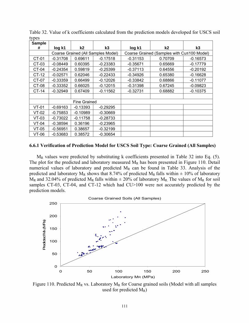
111

Table 32. Value of k coefficients calculated from the prediction models developed for USCS soil types

Sample # log k1 k2 k3 log k1 k2 k3 Coarse Grained (All Samples Model) Coarse Grained (Samples with Cu≤100 Model)

CT-01 -0.31708 0.69611 -0.17518 -0.31153 0.70709 -0.16573 CT-03 -0.08449 0.60395 -0.23383 -0.35671 0.65669 -0.17779 CT-04 -0.24354 0.59819 -0.25399 -0.37113 0.64556 -0.20192 CT-12 -0.02571 0.62046 -0.22433 -0.34926 0.65380 -0.16628 CT-07 -0.33359 0.66499 -0.12026 -0.33842 0.68866 -0.11077 CT-08 -0.33352 0.66025 -0.12015 -0.31398 0.67245 -0.09823 CT-14 -0.32949 0.67409 -0.11562 -0.32731 0.68882 -0.10375

Fine Grained

VT-01 -0.69163 -0.13393 -0.29295 VT-02 -0.75853 -0.10989 -0.30669 VT-03 -0.73022 -0.11758 -0.28733 VT-04 -0.38594 0.36196 -0.23965 VT-05 -0.56951 0.38657 -0.32199 VT-06 -0.53683 0.38572 -0.30654

6.6.1 Verification of Prediction Model for USCS Soil Type: Coarse Grained (All Samples)

MR values were predicted by substituting k coefficients presented in Table 32 into Eq. (5). The plot for the predicted and laboratory measured MR has been presented in Figure 110. Detail numerical values of laboratory and predicted MR can be found in Table 33. Analysis of the predicted and laboratory MR shows that 8.74% of predicted MR falls within ± 10% of laboratory MR and 32.04% of predicted MR falls within ± 20% of laboratory MR. The values of MR for soil samples CT-03, CT-04, and CT-12 which had CU>100 were not accurately predicted by the prediction models.

Coarse Grained Soils (All Samples)

0

50

100

150

200

250


Pre

dict

ed M

R (M

Pa)

Figure 110. Predicted MR vs. Laboratory MR for Coarse grained soils (Model with all samples

used for predicted MR)

112

6.6.2 Verification of Prediction Model for USCS Soil Type: Coarse Grained (Samples with CU≤100)

MR values were predicted by substituting k coefficients presented in Table 32 into Eq. (5). Plot for predicted MR calculated using prediction models developed from coarse grained soil samples that have CU≤100 and laboratory MR has been presented in Figure111. Detail numerical values of laboratory and predicted MR can be found in Table 33. Evaluation of the MR values show that 22.33% of predicted MR values were within ± 10% of the laboratory MR values and 68.93% of predicted MR values were within ± 20% of the laboratory MR values.

Coarse Grained Soils (Samples with CU<100)

0

50

100

150

200

250


Pred

icte

d M

R (M

Pa)

Figure 111. Predicted MR vs. Laboratory MR for Coarse grained soils (Model with all samples

that had CU≤100 used for predicted MR)

113

Table 33. Comparison of Laboratory and Predicted MR values for Coarse Grained soils Predicted MR

Lab MR

From Model with all samples

From Model with samples that

had CU≤100 Sample # MPa MPa MPa

CT-01 90 99.05 97.98 CT-01 95 93.13 92.81 CT-01 96 91.74 91.86 CT-01 97 91.86 92.31 CT-01 98 92.66 93.37 CT-01 66 77.12 75.97 CT-01 67 74.35 73.82 CT-01 71 74.65 74.5 CT-01 76 75.99 76.13 CT-01 78 77.77 78.15 CT-01 45 51.78 50.69 CT-01 47 52.92 52.27 CT-01 51 55.55 55.18

CT-04 92 142.24 92.75 CT-04 86 125.84 85.4 CT-04 77 119.2 82.91 CT-04 74 115.86 82.09 CT-04 72 114.07 82.04 CT-04 79 114.74 73.55 CT-04 70 103.68 69.27 CT-04 64 99.87 68.49 CT-04 62 98.46 68.86 CT-04 62 98.14 69.74 CT-04 57 81.68 50.91 CT-04 51 77.57 50.59 CT-04 48 77.5 52.06 CT-04 48 78.64 54 CT-04 50 80.22 56.09

Predicted MR

Lab MR






114

Table 33. Comparison of Laboratory and Predicted MR values for Coarse Grained soils (Cont’d…)

Predicted MR

Lab MR





CT-08 67 80.57 79.48 CT-08 70 78.59 78.8 CT-08 71 78.95 79.95 CT-08 72 80.09 81.68 CT-08 74 81.66 83.76 CT-08 54 63.5 62.37 CT-08 54 63.43 63.35 CT-08 56 65.01 65.6 CT-08 59 67 68.11 CT-08 60 69.18 70.74 CT-08 36 43.58 42.48 CT-08 37 46 45.65 CT-08 40 49.16 49.33 CT-08 39 52.23 52.83 CT-08 29 55.03 56

6.6.3 Verification of Prediction Model for USCS Soil Type: Fine Grained

MR values were predicted by substituting k coefficients for fine grained soil presented in Table 32 into Eq. (5). Plot for predicted MR against laboratory MR has been presented in Figure 112. Numerical values of laboratory and predicted MR can be found in Table 34. Evaluation of the MR values show that 37.78% of predicted MR values were within ± 10% of the laboratory MR values and 54.44% of predicted MR values were within ± 20% of the laboratory MR. The MR values for soil samples VT-01, VT-02, VT-03 which had PI and LL values much higher than the

Predicted MR

Lab MR





115

PI and LL values used in developing prediction models had larger error values, hence warning against extrapolation.

Table 34. Comparison of Laboratory and Predicted MR values for Fine Grained soils

Lab MR Predicted MR Sample # MPa MPa

VT-01 70 45.56 VT-01 69 36.77 VT-01 65 32.34 VT-01 61 29.48 VT-01 58 27.38 VT-01 65 47.86 VT-01 64 38.43 VT-01 61 33.68 VT-01 58 30.6 VT-01 56 28.32 VT-01 50 51.76 VT-01 53 41.12 VT-01 54 35.69 VT-01 53 32.2 VT-01 52 29.66





116

Table 34. Comparison of Laboratory and Predicted MR values for Fine Grained soils (Cont’d…) Lab MR Predicted MR Sample

# MPa MPa VT-05 79 76.45 VT-05 74 63.18 VT-05 66 57.41 VT-05 62 53.89 VT-05 59 51.53 VT-05 71 66.51 VT-05 64 55.86 VT-05 58 51.25 VT-05 54 48.55 VT-05 53 46.76 VT-05 56 53.5 VT-05 51 46.42 VT-05 47 43.58 VT-05 45 42.03 VT-05 45 41.08

Fine Grained Soils

0

50

100

150

200

250


Pred

icte

d M

R (M

Pa)

Figure 112. Predicted MR vs. Laboratory MR for Fine grained soils


VT-06 81 78.93 VT-06 75 66 VT-06 67 60.25 VT-06 62 56.79 VT-06 60 54.46 VT-06 73 68.68 VT-06 65 58.31 VT-06 58 53.78 VT-06 54 51.15 VT-06 52 49.43 VT-06 57 55.12 VT-06 51 48.42 VT-06 47 45.71 VT-06 45 44.31 VT-06 44 43.46

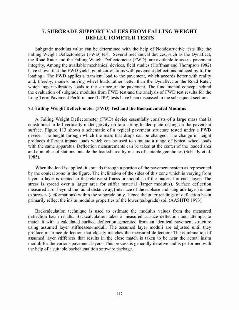
117

7. SUBGRADE SUPPORT VALUES FROM FALLING WEIGHT DEFLECTOMETER TESTS

Subgrade modulus value can be determined with the help of Nondestructive tests like the

Falling Weight Deflectometer (FWD) test. Several mechanical devices, such as the Dynaflect, the Road Rater and the Falling Weight Deflectometer (FWD), are available to assess pavement integrity. Among the available mechanical devices, field studies (Hoffman and Thompson 1982) have shown that the FWD yields good correlations with pavement deflections induced by traffic loading. The FWD applies a transient load to the pavement, which accords better with reality and, thereby, models moving wheel loads rather better than the Dynaflect or the Road Rater, which impart vibratory loads to the surface of the pavement. The fundamental concept behind the evaluation of subgrade modulus from FWD test and the analysis of FWD test results for the Long Term Pavement Performance (LTPP) tests have been discussed in the subsequent sections.

7.1 Falling Weight Deflectometer (FWD) Test and the Backcalculated Modulus

A Falling Weight Deflectometer (FWD) device essentially consists of a large mass that is

constrained to fall vertically under gravity on to a spring loaded plate resting on the pavement surface. Figure 113 shows a schematic of a typical pavement structure tested under a FWD device. The height through which the mass that drops can be changed. The change in height produces different impact loads which can be used to simulate a range of typical wheel loads with the same apparatus. Deflection measurements can be taken at the center of the loaded area and a number of stations outside the loaded area by means of suitable geophones (Sebaaly et al. 1985).

When the load is applied, it spreads through a portion of the pavement system as represented

by the conical zone in the figure. The inclination of the sides of this zone which is varying from layer to layer is related to the relative stiffness or modulus of the material in each layer. The stress is spread over a larger area for stiffer material (larger modulus). Surface deflection measured at or beyond the radial distance a3e (interface of the subbase and subgrade layer) is due to stresses (deformations) within the subgrade only. Hence the outer readings of deflection basin primarily reflect the insitu modulus properties of the lower (subgrade) soil (AASHTO 1993).

Backcalculation technique is used to estimate the modulus values from the measured

deflection basin results. Backcalculation takes a measured surface deflection and attempts to match it with a calculated surface deflection generated from an identical pavement structure using assumed layer stiffnesses/moduli. The assumed layer moduli are adjusted until they produce a surface deflection that closely matches the measured deflection. The combination of assumed layer stiffeness that results in the close match is taken to be near the actual insitu moduli for the various pavement layers. This process is generally iterative and is performed with the help of a suitable backcalcualtion software package.

118

Figure 113. Schematic of Stress Zone within Pavement Structure under the FWD Load (AASHTO 1993) 7.2 Comparison of Laboratory Resilient Modulus (MR) and FWD Backcalculated Modulus

To correlate the laboratory resilient modulus (MR) values and FWD backcalculated modulus (E (FWD)) values, the test data for 20 states in the United States and 2 Provinces in Canada within the 4 regions, namely, New England, Northern Mid Atlantic, Great Lakes and Upper Mid West, was extracted from Long Term Pavement Perfromance (LTPP) Information Management System (IMS) Data, Release 15, January 2003 Upload. All raw data extracted from LTPP database has been presented in Appendix I (available in CD). The LTPP test sites where Laboratory resilient modulus (MR) and field (FWD) tests are available have been presented in Appendix B, Table B.1. In the table, the test sites where both the MR and FWD data were collected by the LTPP program are shown in bold type face. SHRP ID in the table is the test section identification number assigned by the LTPP program. It must be combined with State Code to be unique. Generally, the field test sections are 152 meter long with a 15.2 meter materials sampling section at each end. For each drop of the mass, deflections were recorded at 7 points to get the deflection bowl. FWD Backcalculated modulus data for Rhode Island is not available in the LTPP database. Mean Elastic Modulus has been calculated using Backcalculation software MODCOMP v 4.2.

For the comparison purpose herein, an average of FWD backcalculated elastic modulus

values corresponding to different levels of drop heights was calculated to obtain a single modulus value for the subgrade soil at a particular test section. They are given in Appendix H,

119

Table H.3.1 through Table H.3.4. Ranges of the E(FWD) to MR ratios at each of the 3 levels of confining pressures for various AASHTO soil types found in the 4 regions (20 states in the U.S. and 2 Provinces in Canada) are presented in Table H.1 in Appendix H. Also, the ranges of the E (FWD) to MR ratios by AASHTO soil types for each of the 20 individual states in the U.S. and 2 Provinces in Canada are given in Tables H.2, H.3, H.4 in Appendix H. Resilient modulus (MR) value considered for Tables H.2, H.3, H.4 are average MR values at confining pressures of 13.8 kPa, 27.6 kPa and 41.4 kPa respectively during laboratory testing. However, the backcalculated modulus values used for calculating the ratio in Tables H.2, H.3, H.4 are the same for all 3 tables.

In general, it was observed that the backcalculated modulus values were higher than the

laboratory resilient modulus values conducted at the same test site. However, these ratios are not showing a definite relationship between the two values. This may be because though at the same test site, the year of FWD testing and lab specimen sampling are different, the moisture content and density during these two tests may be different, etc. Furthermore, since MR depends on soil and stress conditions, calculating the ratio E(FWD)/Lab MR under different lab stress conditions against a single field stress condition may have resulted inaccurate values of ratios.

A better approach would have been to calculate the MR using bulk and octahedral stresses at

the depth of representative subgrade D where the stress ratio (normal stress at the pavement surface / the normal stress at the depth, D) is less than or equal to 0.1 and compare this MR with the backcalculated MR. Knowing the k coefficients for each type of soil for each LTPP site, the bulk and octahedral stresses at D, MR can be calculated using Eq. (2). Due to the unavailability of data on field stress conditions, this approach could not be used.

120

8. SUMMARY AND CONCLUSIONS

The main objective of this research project was to establish subgrade support (resilient modulus) values for typical soils in New England. To accomplish this goal, various publications and database were used. These include United States Department of Agriculture (USDA) Soil Survey reports, Long Term Pavement Performance Information Management System (LTPP IMS) database, Transportation Research Information Services (TRIS) database and several other reports and journal articles.

From the thorough review of USDA soil survey reports, we identified the major soil types

found in the New England States. These include A-1, A-2, A-3, A-4, A-5, A-6 and A-7 soil types. Connecticut has A-2 and A-4, Maine has A-1, A-2, A-3, A-4 A-5 and A-6, Massachusetts has A-1, A-2, A-3, A-4, A-5 and A-6, New Hampshire has A-1, A-2 and A-4, Vermont has A-1, A-2, A-4, A-6 and A-7 as the predominant soil types. The predominant soil type in Rhode Island could not be identified because the soil type for only the entire state has been given but not county wise.

The data collected on laboratory resilient modulus tests for about 300 LTPP test sites in 21

different states from LTPP IMS database show that the resilient modulus value generally increases with the increase in confining pressure during the test for the AASHTO soil types A-1-b, A-3, A-2-4, A-4, A-6 and A-7-6. Soil types A-1-a, A-2-5, A-2-7, A-5 and A-7-5 were not present in the test sites considered for this study. It was observed that for the granular soils like A-1-b, A-3, and A-2-4, MR usually increased with increase in nominal maximum axial stress at the same level of confining pressure while for silty-clay soils like A-4, A-6, and A-7-6 there was a general trend of decrease in MR with increase in nominal maximum axial stress at the same level of confining pressure. Observation of MR values for the test sites considered from LTPP IMS database show that for A-1-b soils, the majority of MR values were in the range of 50 to 110 MPa. Likewise, for A-3 soils the range is 50 to 110 MPa, for A-2-4 soils the range is 50 to 120 MPa, for A-2-6 soils the range is 50 to 120 MPa, for A-4 soils the range is 30 to 150, for A-6 soils the range is 30 to 160 MPa and for A-7-6 soils, the range is 20 to 150 MPa. It was observed that the minimum resilient modulus values obtained for A-1-b, A-3, A-2-4 soils were higher than the minimum values for A-4, A-6 and A-7-6 soils.

Generalized constitutive model that relates resilient modulus (MR) with the bulk stress and

octahedral shear stress was considered for predicting the subgrade MR by developing regression equations for the k coefficients in the model. The regression equations relate the k coefficients to the soil properties which makes the prediction of MR possible based on these basic soil properties at known stress states. Prediction models for the k coefficients in the generalized constitutive model were developed for AASHTO soil types A-1-b, A-3, A-2-4, A-4, A-6, and A-7-6 using multiple linear regression technique. The data used for model development were collected from LTPP IMS database for 259 test specimens collected from test sites in 21 states including 3 New England states, 16 nearby states in the U.S. and 2 provinces in Canada. Three prediction models have been developed for each AASHTO soil type. The first set of model is the composite model that has been developed from all reconstituted soil specimens, the second set of models have been developed from only those samples that had been compacted at the optimum moisture content during MR testing and the third model set of models have been developed from the

121

samples that had been compacted at insitu moisture content. In the regression analysis, the multiple correlation coefficient (R2), adjusted R2, Variance Inflation Factor (VIF) and the consideration of relevant soil physical properties were the criteria used for selecting an appropriate model for the k coefficients. Summary of the prediction models developed are presented in Table 35 through Table 40. The R2 values obtained for the prediction models for k coefficients relating to the soil properties lie between 0.30 and 0.99. Descriptive statistics that compare the prediction models with the measured data are summarized in Table 42.

Furthermore, the data collected from LTPP database were classified according to Unified

Soil Classification System into Coarse Grained and Fine Grained soils and prediction models were developed for each type. Summary of the prediction models developed for the USCS soil types are presented in Table 41. The R2 values for the models ranged from 0.22 to 0.63. Descriptive statistics that compare the prediction models with the measured data are summarized in Table 42.

Some R2 values are not as high as reported in some of the previous studies since the data

extracted from the LTPP database for this study covered varied and wide locations. Also, the resilient modulus tests in the LTPP database were not performed in a single laboratory. This introduces high possibility of variations in the measure data due to equipment/operator variability. Since the models in this study were developed from a large number of samples covering 19 different states in the U.S. and 2 provinces in Canada, these models should be applicable to a wider geographic region.

The results from the laboratory MR tests conducted on representative New England subgrade

soils show that for both AASHTO and USCS soil type categories, the MR values obtained from the prediction models developed in this study matched reasonably well in general, and in some case quite close, to the experimental values. The descriptive statistics showing the comparison between the MR values from the prediction models and that from the laboratory tests have been summarized in Table 43.

It was observed that extrapolating beyond the range of predictor variables yielded large

errors between the predicted and laboratory MR values. Therefore, care should be taken while using the developed prediction models to predict MR values of new samples so as to avoid extrapolation beyond the values of predictor variables used in developing the models.

In general, the FWD backcalculated values obtained from LTPP IMS database were observed

to be higher than the laboratory resilient modulus values at the same site. However, a definite relationship between these two values could not be observed due to large variations in the FWD backcalculated modulus values and the lack of data of these two types of tests performed under similar conditions of moisture, density, and season and data on field stress.

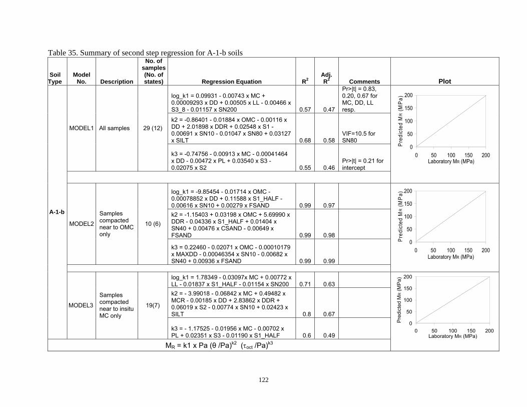
122

Table 35. Summary of second step regression for A-1-b soils

Soil Type

Model No. Description

No. of samples (No. of states) Regression Equation R2

Adj. R2 Comments Plot

log_k1 = 0.09931 - 0.00743 x MC + 0.00009293 x DD + 0.00505 x LL - 0.00466 x S3_8 - 0.01157 x SN200 0.57 0.47

Pr>|t| = 0.83, 0.20, 0.67 for MC, DD, LL resp.

k2 = -0.86401 - 0.01884 x OMC - 0.00116 x DD + 2.01898 x DDR + 0.02548 x S1 - 0.00691 x SN10 - 0.01047 x SN80 + 0.03127 x SILT 0.68 0.58

VIF=10.5 for SN80

MODEL1 All samples 29 (12)

k3 = -0.74756 - 0.00913 x MC - 0.00041464 x DD - 0.00472 x PL + 0.03540 x S3 - 0.02075 x S2 0.55 0.46

Pr>|t| = 0.21 for intercept

log_k1 = -9.85454 - 0.01714 x OMC - 0.00078852 x DD + 0.11588 x S1_HALF - 0.00616 x SN10 + 0.00279 x FSAND 0.99 0.97 k2 = -1.15403 + 0.03198 x OMC + 5.69990 x DDR - 0.04336 x S1_HALF + 0.01404 x SN40 + 0.00476 x CSAND - 0.00649 x FSAND 0.99 0.98

MODEL2

Samples compacted near to OMC only

10 (6)

k3 = 0.22460 - 0.02071 x OMC - 0.00010179 x MAXDD - 0.00046354 x SN10 - 0.00682 x SN40 + 0.00936 x FSAND 0.99 0.99

log_k1 = 1.78349 - 0.03097x MC + 0.00772 x LL - 0.01837 x S1_HALF - 0.01154 x SN200 0.71 0.63 k2 = - 3.99018 - 0.06842 x MC + 0.49482 x MCR - 0.00185 x DD + 2.83862 x DDR + 0.06019 x S2 - 0.00774 x SN10 + 0.02423 x SILT 0.8 0.67

A-1-b

MODEL3

Samples compacted near to insitu MC only

19(7)

k3 = - 1.17525 - 0.01956 x MC - 0.00702 x PL + 0.02351 x S3 - 0.01190 x S1_HALF 0.6 0.49

MR = k1 x Pa (θ /Pa)k2 (τoct /Pa)k3

0

50

100

150

200


Pre

dict

ed M

R (M

Pa)

0

50

100

150

200


Pre

dict

ed M

R (M

Pa)

0

50

100

150

200


Pred

icte

d M

R (M

Pa)

123

Table 36. Summary of second step regression for A-3 soils

Soil Type




log_k1 = - 0.93681 - 0.01248 x MC + 0.30352 x MCR + 0.00020285 x DD + 0.00194 x FSAND 0.47 0.32

Pr>|t|=0.24 for DD

k2 = - 0.13234 - 0.01724 x MC + 0.02560 x OMC + 0.00032543 x DD + 0.00313 x SN40 - 0.00291x SN80 - 0.01843 x CLAY 0.58 0.38

Pr>|t|=0.82 & 0.28 for intercept & DD


k3 = - 1.03002 + 0.09865 x MCR + 0.00032615 x DD + 0.00220 x S1_HALF + 0.00067403 x SN40 0.76 0.69

log_k1 = -1.28763 - 0.01554 x OMC - 1.59688 x DDR + 0.04783 x S1 - 0.02146 x S3_4 + 0.00124 x SN80 0.72 0.55

Pr>|t|=0.35 for intercept

k2 = -5.81794 + 0.00420 x OMC + 0.42100 x MCR - 2.53496 x DDR + 0.06786 x S1_HALF + 0.01649 x S3_4 0.8 0.67

Pr>|t|=0.26, 0.36 & 0.18 for OMC, MCR & S3_4 resp. MODEL2


14 (10)

k3 = - 0.78512 + 0.00270 x OMC + 0.00032286 x DD + 0.04002 x S1_HALF - 0.04000 x S1 + 0.00119 x SN40 - 0.00077438 x SN80 + 0.00446 x SILT 0.99 0.98

log_k1 = - 1.80028 + 0.06083 x MC + 0.09612 x OMC 0.99 0.99

k2 = 1.11468 - 0.03964 x MC - 0.04803 x CLAY 0.98 0.94

A-3

MODEL3


4 (3)

k3 = 1.89076 - 0.08899 x OMC - 0.00055406 x MAXDD 0.99 0.99

Only 4 samples, models to be used with caution


0

50

100

150

200


Pre

dict

ed M

R (M

Pa)

0

50

100

150

200


Pre

dict

ed M

R (M

Pa)

0

50

100

150

200


Pre

dict

ed M

R (M

Pa)

124

Table 37. Summary of second step regression for A-2-4 soils

Soil Type




log_k1 = 1.10795 - 0.02889 x OMC - 0.23628 x MCR - 0.67002 x DDR - 0.01701 x S2 + 0.01405 x S3_4 0.37 0.28 k2 = - 0.69772 + 0.02106 x MC + 0.00054260 x DD - 0.00657 x LL + 0.00293 x SN10 - 0.00460 x SN200 0.58 0.51 MODEL1 All samples 40 (13)

k3 = 0.50825 - 0.01956 x OMC - 0.07234 x MCR - 0.00492 x LL - 0.00652 x S2 + 0.00384 x SN40 - 0.00153 x SN80 + 0.00344 x CLAY 0.69 0.63

log_k1 = 2.01010 - 0.06696 x OMC + 0.00057415 x DD - 0.00095144 x MAXDD - 0.04473 x S2 + 0.03673 x S1 - 0.00355 x CSAND 0.59 0.48

Pr>|t|=0.21 for CSAND

k2 = 2.05743 + 0.02542 x OMC - 2.57064 x DDR + 0.08047 x S2 - 0.09125 x S1 + 0.01852 x S3_8 - 0.00776 x SN200 + 0.01014 x CSAND 0.78 0.7

MODEL2


28 (12)

k3 = 1.79954 - 0.05488 x MC - 0.00061034 x MAXDD - 0.00592 x LL - 0.00917 x S2 + 0.00751 x S1_2 - 0.00288 x CSAND + 0.00440 x CLAY 0.86 0.81

log_k1 = 1.05873 - 0.13450 x MCR + 0.00045768 x MAXDD - 0.00905 x LL - 0.02172 x S3 + 0.00269 x SN80 - 0.00982 x SILT 0.99 0.98 k2 = - 1.58669 + 0.01953 x OMC + 0.00036406 x DD + 0.01688 x S1_2 - 0.00949 x SN80 - 0.01289 x CSAND + 0.02220 x SILT 0.99 0.97

A-2-4

MODEL3


12 (6)

k3 = - 1.26595 + 0.01043 x MC + 0.00070217 x DD - 0.01068 x SN200 - 0.00971 x CSAND 0.79 0.66


0

50

100

150

200


Pre

dict

ed M

R (M

Pa)

0

50

100

150

200


Pred

icte

d M

R (M

Pa)

0

50

100

150

200


Pred

icte

d M

R (M

Pa)

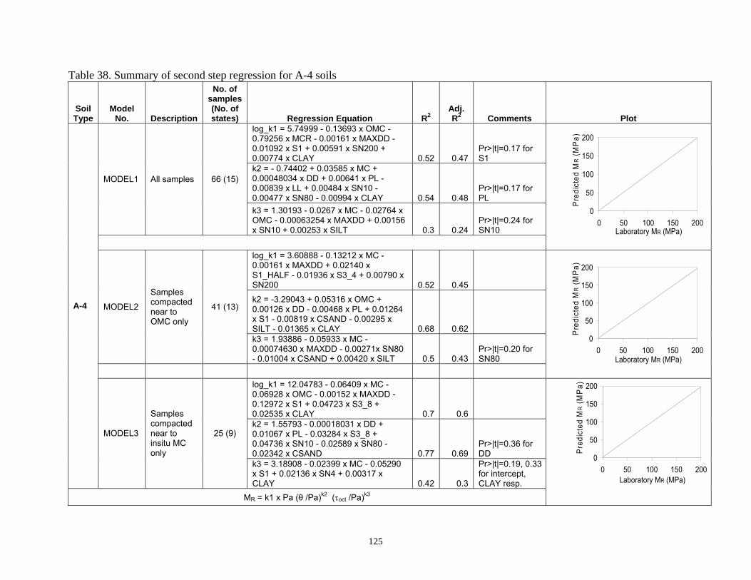
125


Soil Type




log_k1 = 5.74999 - 0.13693 x OMC - 0.79256 x MCR - 0.00161 x MAXDD - 0.01092 x S1 + 0.00591 x SN200 + 0.00774 x CLAY 0.52 0.47

Pr>|t|=0.17 for S1

k2 = - 0.74402 + 0.03585 x MC + 0.00048034 x DD + 0.00641 x PL - 0.00839 x LL + 0.00484 x SN10 - 0.00477 x SN80 - 0.00994 x CLAY 0.54 0.48

Pr>|t|=0.17 for PL


k3 = 1.30193 - 0.0267 x MC - 0.02764 x OMC - 0.00063254 x MAXDD + 0.00156 x SN10 + 0.00253 x SILT 0.3 0.24

Pr>|t|=0.24 for SN10

log_k1 = 3.60888 - 0.13212 x MC - 0.00161 x MAXDD + 0.02140 x S1_HALF - 0.01936 x S3_4 + 0.00790 x SN200 0.52 0.45

k2 = -3.29043 + 0.05316 x OMC + 0.00126 x DD - 0.00468 x PL + 0.01264 x S1 - 0.00819 x CSAND - 0.00295 x SILT - 0.01365 x CLAY 0.68 0.62

MODEL2


41 (13)

k3 = 1.93886 - 0.05933 x MC - 0.00074630 x MAXDD - 0.00271x SN80 - 0.01004 x CSAND + 0.00420 x SILT 0.5 0.43

Pr>|t|=0.20 for SN80

log_k1 = 12.04783 - 0.06409 x MC - 0.06928 x OMC - 0.00152 x MAXDD - 0.12972 x S1 + 0.04723 x S3_8 + 0.02535 x CLAY 0.7 0.6 k2 = 1.55793 - 0.00018031 x DD + 0.01067 x PL - 0.03284 x S3_8 + 0.04736 x SN10 - 0.02589 x SN80 - 0.02342 x CSAND 0.77 0.69

Pr>|t|=0.36 for DD

A-4

MODEL3


25 (9)

k3 = 3.18908 - 0.02399 x MC - 0.05290 x S1 + 0.02136 x SN4 + 0.00317 x CLAY 0.42 0.3

Pr>|t|=0.19, 0.33 for intercept, CLAY resp.


0

50

100

150

200


Pred

icte

d M

R (M

Pa)

0

50

100

150

200


Pre

dict

ed M

R (M

Pa)

0

50

100

150

200


Pre

dict

ed M

R (M

Pa)

126


Soil Type




log_k1 = 4.59815 - 0.12918 x MC - 0.00211 x MAXDD + 0.04246 x LL - 0.01500 x CSAND - 0.01746 x CLAY 0.52 0.44

Pr>|t|=0.30 for CSAND

k2 = - 2.54229 + 0.00971 x MC + 0.00122 x MAXDD + 0.02703 x SN40 - 0.02122 x SN200 - 0.02393 x FSAND 0.47 0.38

Pr>|t|=0.48 for MC, VIF=18, 31 for SN40, SN200 resp.


k3 = 2.08649 - 0.05214 x MC - 0.00071714 x MAXDD + 0.02450 x LL - 0.01231 x S1 + 0.00493 x SN80 - 0.00922 x CLAY 0.49 0.38

Pr>|t|=0.19, 0.22, 0.21 for intercept, MAXDD, S1 resp.

log_k1 = 11.43172 - 0.11840 x MC + 0.07733 x PL + 0.03185 x LL - 0.16290 x S2 + 0.04052 x SN4 0.58 0.45 k2 = - 3.39047 - 0.00037458 x MAXDD - 0.01423 x LL + 0.06384 x S2 - 0.01620 x SN4 0.45 0.32 Pr<W=0.0214

MODEL2


23 (12)

k3 = 5.70946 - 0.05880 x MC + 0.04341 x PL + 0.01976 x LL - 0.08633 x S2 + 0.02200 x SN4 0.55 0.42


log_k1 = 17.64679 - 0.00330 x MAXDD - 0.17669 x PL - 0.10358 x S1_2 + 0.04379 x CLAY 0.78 0.66 k2 = 0.35299 - 0.03880 x OMC + 0.08025 x PL - 0.04909 x LL + 0.00939 x SN80 0.8 0.71


A-6

MODEL3


13 (6)

k3 = 8.60279 - 0.00107 x DD - 0.06858 x PL - 0.06568 x S3_4 + 0.01672 x SN80 - 0.01271 x SILT 0.68 0.46

VIF=12.3 for SN80


0

50

100

150

200

250


Pred

icte

d M

R (M

Pa)

0

50

100

150

200

250


Pred

icte

d M

R (M

Pa)

0

50

100

150

200

250


Pred

icte

d M

R (M

Pa)

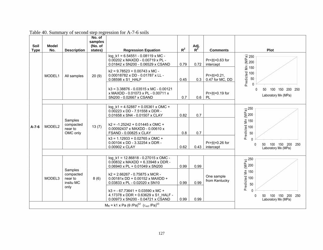
127

Table 40. Summary of second step regression for A-7-6 soils

Soil Type



Adj. R2 Comments

Plot log_k1 = 6.54551 - 0.08119 x MC - 0.00202 x MAXDD - 0.00719 x PL - 0.01842 x SN200 - 0.06529 x CSAND 0.79 0.72


k2 = 9.78523 + 0.00743 x MC - 0.00018782 x DD - 0.01787 x LL - 0.08598 x S1_HALF 0.45 0.3

Pr>|t|=0.21, 0.47 for MC, DD


k3 = 3.38876 - 0.03515 x MC - 0.00121 x MAXDD - 0.01073 x PL - 0.00711 x SN200 - 0.02667 x CSAND 0.7 0.6

Pr>|t|=0.19 for PL

log_k1 = 4.52887 + 0.05361 x OMC + 0.00223 x DD - 7.51558 x DDR - 0.01658 x SN4 - 0.01507 x CLAY 0.82 0.7

k2 = -1.25242 + 0.01445 x OMC + 0.00092437 x MAXDD - 0.00610 x FSAND - 0.00825 x CLAY 0.8 0.7

MODEL2


13 (7)

k3 = 1.12933 + 0.02765 x OMC + 0.00104 x DD - 3.32254 x DDR - 0.00902 x CLAY 0.62 0.43


log_k1 = 12.86818 - 0.27015 x OMC - 0.00832 x MAXDD + 6.33948 x DDR - 0.06940 x PL + 0.01049 x SN200 0.99 0.99

k2 = 2.66267 - 0.75875 x MCR - 0.00181x DD + 0.00152 x MAXDD + 0.03833 x PL - 0.02020 x SN10 0.99 0.99

A-7-6

MODEL3


8 (6)

k3 = - 67.73641 + 0.03590 x MC + 4.17378 x DDR + 0.63629 x S1_HALF - 0.00973 x SN200 - 0.04721 x CSAND 0.99 0.99

One sample from Kentucky


050

100150200250


Pred

icte

d M

R (M

Pa)

0

50

100

150

200

250


Pred

icte

d M

R (M

Pa)

0

50

100

150

200

250


Pre

dict

ed M

R (M

Pa)

128

Table 41. Summary of second step regression for USCS soil types

Soil Type

No. of samples (No.

of states) Regression Equation R2 Adj. R2 Comments Plot

logk1 = -1.77341 + 0.00017562xMAXDD + 0.02707xS3 - 0.02043xS1 + 0.00501xS3_8 - 0.00819xSN200 + 0.00501xSILT 0.4 0.36 Pr<W=0.12

k2 = -0.49426 + 0.11250xMCR + 0.00026190xDD + 0.00592xS3 - 0.00398xSN40 + 0.00479xFSAND - 0.00006099xCU - 0.0000967xCC 0.45 0.41

Pr>|t|=0.31, 0.29 for intercept & CC

Coarse Grained

(All Samples)

91 (19)

k3 = -0.44082 - 0.00232xMC + 0.00021026xMAXDD - 0.00531xS1_2 + 0.00561 xSN10 - 0.00529xSN200 0.63 0.61

Pr>|t|=0.31 for MC, Pr<W=0.085

logk1 = 0.61689 - 0.00815xOMC - 0.06144xMCR - 0.80003xDDR - 0.00878xSN200 + 0.00624xSILT + 0.00621xCLAY - 0.00502xCC 0.47 0.41

k2 = 0.43372 + 0.00687xMC + 0.00039979xDD - 0.00026666xMAXDD - 0.00331xSN40 + 0.00297xFSAND + 0.00515xCC 0.22 0.15


Coarse Grained

(Samples with

CU≤100))

74 (17)

k3 = 0.51731 - 0.00390xMC - 0.43830xDDR - 0.00594xS1_2 + 0.00509xSN10 - 0.00070032xSN40 - 0.00418xSN200 + 0.00441xCLAY 0.52 0.47 Pr<W=0.0164

logk1 = 6.99969 - 0.11144xOMC - 1.15320xMCR - 0.00154xMAXDD + 0.01875 x PI - 0.02339xS1 + 0.00445xSN200 0.41 0.37 k2 = 0.55494 + 0.25904xMCR - 0.00651xPI - 0.00785xSN4 + 0.00712xSN40 - 0.00266xSN200 - 0.00318xCLAY 0.39 0.34 Pr<W<0.0001

Fine Grained 97 (16)

k3 = 2.08483 - 0.03626xMC - 0.00044337xMAXDD + 0.01104xLL - 0.02024xS1 + 0.00494xSN80 + 0.01012xCSAND + 0.00392xFSAND+0.00287xSILT 0.33 0.27


0

50

100

150

200


Pred

icte

d M

R (M

Pa)

0

50

100

150

200


Pred

icte

d M

R (M

Pa)

050

100150200250


Pred

icte

d M

R (M

Pa)

129

Table 42. Descriptive statistics for the prediction models

MODEL# * No. of

Samples

No. of MR data

values

Percentage of predicted MR within ±10 % of laboratory

MR

Percentage of predicted MR within ± 20 % of laboratory

MR A-1-b MODEL1 29 432 59.95% 94.21% MODEL2 10 150 96.00% 98.00% MODEL3 19 282 73.05% 98.94% A-3 MODEL1 19 284 63.73% 94.72% MODEL2 14 209 79.43% 98.56% MODEL3 4 60 100% 100 A-2-4 MODEL1 40 600 51.33% 84.33% MODEL2 28 420 64.29% 89.29% MODEL3 12 180 85.56% 100% A-4 MODEL1 66 988 35.53% 62.15% MODEL2 41 614 35.83% 66.29% MODEL3 25 374 39.04% 73.79% A-6 MODEL1 36 540 22.59% 42.96% MODEL2 23 345 33.62% 57.10% MODEL3 13 195 41.03% 70.26% A-7-6 MODEL1 20 300 36.33% 66.33% MODEL2 13 195 67.18% 95.38% MODEL3 8** 120 95.83% 100% Coarse Grained All samples 91 1359 50.04% 77.63% Samples with Cu≤100 74 1109 60.32% 85.75%

Fine Grained 97 1455 30.03% 50.86%

* MODEL1 – Prediction Models developed with all reconstituted samples MODEL2 – Prediction Models developed with samples compacted at optimum moisture

content only MODEL3 – Prediction Models developed with samples compacted at insitu moisture content

only ** One additional sample from Kentucky

130

Table 43. Descriptive statistics for the validation of prediction models

MODEL# * No. of

Samples

No. of MR data values

Percentage of predicted MR within ±10 % of laboratory

MR

Percentage of predicted MR within ± 20 % of laboratory

MR A-1-b MODEL1 3 45 90.00% 100.00% A-3 MODEL1 3 45 68.89% 97.78% MODEL2 3 45 6.67% 17.78% A-2-4 MODEL1 1 15 40.00% 86.67% MODEL2 1 15 20.00% 40.00% A-4 MODEL1 6 90 58.89% 87.78% MODEL2 6 90 64.44% 83.33% Coarse Grained All Samples 7 103 8.73% 32.04% Samples with Cu≤100 7 103 22.33% 68.93% Fine Grained 6 90 37.78% 54.44%

* MODEL1 – Prediction Models developed with all reconstituted samples MODEL2 – Prediction Models developed with samples compacted at optimum moisture

content only

131

9. REFERENCES AND BIBLIOGRAPHY

1. AASHTO (1993). AASHTO Guide for Design of Pavement Structures, American Association of State Highway and Transportation Officials, Washington, D.C. 2. AASHTO - T 307 (2003). “Determining the Resilient Modulus of Soils and Aggregate Materials.” Standard Specifications for Transportation Materials and Methods of Sampling and Testing, Adopted by the American Association of State Highway and Transportation Officials . 3. 2002 Design Guide, Design of New and Rehabilitated Pavement Structures (2003), Draft, Review Copy), National Cooperative Highway Research Program, National Research Council, Transportation Research Board, Washington, D. C. 4. Ali, N.A., and Khosla, N.P. (1987). “Determination of Layer Moduli using a Falling Weight Deflectometer.”, Transportation Research Record, National Research Council, Washington, D.C., 1117, 1-10. 5. Allen, G.W. (1974). Soil survey of Chittenden County, Vermont, United States Department of Agriculture, Soil Conservation Service in cooperation with Vermont Agricultural Experiment Station and Vermont Department of Forests and Parks, National Cooperative Soil Survey. 6. Arno, J.R. (1964a). Soil survey of Aroostook County, Maine, Northeastern Part, United States Department of Agriculture, Natural Resources Soil Conservation Service in cooperation with University of Maine Agricultural Experiment Station. 7. Arno, J.R. (1964b). Soil survey of Aroostook County, Maine, Southern Part, United States Department of Agriculture, Natural Resources Soil Conservation Service in cooperation with University of Maine Agricultural Experiment Station. 8. Arno, J.R., Willey, R.B., Farley, W.H., Bither, R.A., and Whitney, B.A. (1972). Soil survey of Somerset County, Maine, Southern Part, United States Department of Agriculture, Soil Conservation Service in cooperation with University of Maine Agricultural Experiment Station. 9. Babcock, R.D. (1981). Soil survey of Lamoille County, Vermont, United States Department of Agriculture, Soil Conservation Service in cooperation with Vermont Agricultural Experiment Station and Vermont Agency of Environmental Conservation, National Cooperative Soil Survey. 10. Bond, R.W., and Handler, J.F. (1981). Soil survey of Hillsborough County, New Hampshire, Eastern Part, United States Department of Agriculture, Soil Conservation Service in cooperation with New Hampshire Agricultural Experiment Station. 11. Burczyk, J.M., Ksaibati K., Sprecher R.A., and Farrar M.J. (1995). “Factors Influencing Determination of a Subgrade Resilient Modulus Value.” Transportation Research Record, National Research Council, Washington, D.C., 1462, 72-78.

132

12. Chen, X., Ender, P., Mitchell, M., Eyben, R. and Wells, C. (2004). “Regression with SAS”, UCLA Academy Technology Services, University of California, Los Angeles, CA, http://www.ats.ucla.edu/stat/sas/webbooks/reg (Nov. 17, 2004) 13. Chatterjee, S., and Price, B. (1977). Regression analysis by example, John Wiley and Sons, Inc., New York. 14. Crouch, M.H. (1983). Soil survey of New London County, Connecticut, United States Department of Agriculture, Soil Conservation Service in cooperation with Connecticut Agricultural Experimental Station and Storrs Agricultural Experiment Station, National Cooperative Soil Survey. 15. Dai, S. and Zollars, J. (2002). “Resilient Modulus of Minnesota Road Research Project Subgrade Soil.” Transportation Research Record, National Research Council, Washington, D.C., 1786, 20-28. 16. Daleiden, J.F., Killingsworth, B.M., Simpson, A.L., and Zamora, R. A. (1994). “Analysis of Procedures for Establishing Insitu Subgrade Moduli.” Transportation Research Record, National Research Council, Washington, D.C., 1462, 102-107. 17. Das, B. M. (1999). Principles of Foundation Engineering, Brooks/Cole Publishing Company. 18. Diers, R.W., and Vieira, F.J. (1977). Soil survey of Carroll County Area, New Hampshire, United States Department of Agriculture, Natural Resources Soil Conservation Service in cooperation with New Hampshire Agricultural Experiment Station. 19. Drumm, E.C., Reeves, J., Madgett, M., (1995). Resilient Modulus of Tennessee Subgrades, Phase II: Verification of Prediction Methods - Volume I: Laboratory Test Results and Improvements to the Alternative test Method, Final Report, Tennessee Department of Transportation / Federal Highway Administration, pp. 97 20. Elkins, G.E., Schmalzer, P., Thompson, T., and Simpson, A. (2003). Long Term Pavement Performance Information Management System, Pavement Performance Database User Guide, Final Report, FHWA-RD-03-088. Federal Highway Administration, United States Department of Transportation. 21. Faust, A.P., and Laflamme, K.J. (1978). Soil survey of Kennebec County, Maine, United States Department of Agriculture, Soil Conservation Service in cooperation with Maine Agricultural Experiment Station and Maine Soil and Water Conservation Commission. 22. Fletcher, P.C. (1993). Soil survey of Barnstable County, Massachusetts, Central Part, United States Department of Agriculture, Soil Conservation Service in cooperation with Massachusetts Agricultural Experiment Station.

133

23. Fletcher, P.C., and Roffinolli, R.J. (1986). Soil survey of Dukes County, Massachusetts, Southern Part, United States Department of Agriculture, Soil Conservation Service in cooperation with Massachusetts Agricultural Experiment Station. 24. Flewelling, L.R., and Lisante, R.H. (1982). Soil survey of York County, Maine, United States Department of Agriculture, Soil Conservation Service in cooperation with Maine Agricultural Experiment Station and Maine Soil and Water Conservation Commission. 25. Flynn, D.J., and Joslin, R.V. (1979). Soil survey of Franklin County, Vermont, United States Department of Agriculture, Soil Conservation Service in cooperation with Vermont Agricultural Experiment Station and Vermont Agency of Environmental Conservation, National Cooperative Soil Survey. 26. Fuller, D.C., and Francis, E. L. (1984). Soil survey of Essex County, Massachusetts, Southern Part, United States Department of Agriculture, Soil Conservation Service in cooperation with Massachusetts Agricultural Experiment Station. 27. Fuller, D.C., and Hotz, C.F. (1981). Soil survey of Essex County, Massachusetts, Northern Part, United States Department of Agriculture, Soil Conservation Service in cooperation with Massachusetts Agricultural Experiment Station. 28. George, K. P. (2004). Prediction of Resilient Modulus from Soil Index Properties, Report No. MS-DOT-RD-04-172, The University of Mississippi in cooperation with The Mississippi Department of Transportation and U.S Department of Transportation, Federal Highway Administration 29. Gonick, W.N., Shearin, A.E., and Hill, D.E. (1970). Soil survey of Litchfield County, Connecticut United States Department of Agriculture, Soil Conservation Service in cooperation with Connecticut Agricultural Experimental Station and Storrs Agricultural Experiment Station, National Cooperative Soil Survey. 30. Goodman, K.V., Riley, R.M., Whitney, B.A., Arno, J.R., La Flamme, K.J., Day, S .V., Hardesty, J.S., Lovejoy, D.B., and Worcester, B. (1963). Soil survey of Penobscot County, Maine, United States Department of Agriculture, Natural Resources Soil Conservation Service in cooperation with University of Maine Agricultural Experiment Station. 31. Griggs, J.E. (1971). Soil survey of Addison County, Vermont, United States Department of Agriculture, Soil Conservation Service in cooperation with Vermont Agricultural Experiment Station and Vermont Agency of Environmental Conservation, National Cooperative Soil Survey. 32. Handler, J.F. (1985). Soil survey of Hillsborough County, New Hampshire, Western Part, United States Department of Agriculture, Soil Conservation Service in cooperation with New Hampshire Agricultural Experiment Station.

134

33. Hedstrom, G.T. (1987). Soil survey of Knox and Lincoln Counties, Maine, United States Department of Agriculture, Soil Conservation Service in cooperation with Maine Agricultural Experiment Station and Maine Soil and Water Conservation Commission. 34. Hedstrom, G.T., and Popp, D.J. (1984). Soil survey of Waldo County, Maine, United States Department of Agriculture, Soil Conservation Service in cooperation with Maine Agricultural Experiment Station and Maine Soil and Water Conservation Commission. 35. Hoffman, M.S., and Thompson, M.R. (1982). “Comparative Study of Selected Nondestructive Testing Devices.” Transportation Research Record, National Research Council, Washington, D.C., 852, 32-41. 36. Hoffman, M.S., and Thompson, M.R. (1982). “Back Calculating Nonlinear Resilient Moduli from Deflection Data.” Transportation Research Record, National Research Council, Washington, D.C., 852, 42-51. 37. Homer, J.W. (1999). Soil survey of Grafton County Area, New Hampshire, United States Department of Agriculture, Natural Resources Soil Conservation Service in cooperation with New Hampshire Agricultural Experiment Station. 38. Houston, W.N., Mamlouck, M.S., and Perera, R. W. S. (1992). “Laboratory versus Nondestructive Testing for Pavement Design.” Journal of Transportation Engineering, 118 (2). 39. Ilgen, L.W., Benton, A.W., Stevens, Jr, K.C., Shearin, A.E., and Hill, D.E. (1966). Soil survey of Tolland County, Connecticut, United States Department of Agriculture, Soil Conservation Service in co-operation with Connecticut Agricultural Experimental Station and Storrs Agricultural Experiment Station, National Cooperative Soil Survey. 40. Janoo, V.C. (1994). Layer Coefficients for NHDOT Pavement Materials, US Army Corps of Engineers, Cold Regions Research & Engineering Laboratory, Special Report 94-30. 41. Janoo, V.C., and Berg, R.L. (1996). PCC Airfield Pavement Response During Thaw-Weakening Periods A Field Study, US Army Corps of Engineers, Cold Regions Research & Engineering Laboratory, Special Report 96-12. 42. Janoo, V.C., Bayer, J.J., Durell, G.D., and Smith Jr, C.E. (1999). Resilient Modulus for New Hampshire Subgrade Soils for Use in Mechanistic AASHTO Design, US Army Corps of Engineers, Cold Regions Research & Engineering Laboratory, Special Report 99-14. 43. Jin, M.S. (1994). “Seasonal Variation of Resilient Modulus of Subgrade Soils”, Journal of Transportation Engineering, ASCE, 120 (4), 603-616. 44. Jordon, G.B. (1998). Soil survey of Honcock County, Maine, United States Department of Agriculture, Natural Resources Soil Conservation Service in cooperation with Maine Agricultural Experiment Station and Maine Soil and Water Conservation Commission.

135

45. Kelsea, R.J., and Gove, J.P. (1994). Soil survey of Rockingham County Area, New Hampshire, United States Department of Agriculture, Natural Resources Soil Conservation Service in cooperation with New Hampshire Agricultural Experiment Station. 46. Kelsey, T.L., and Vieira, F.J. (1968). Soil survey of Belknap County Area, New Hampshire, United States Department of Agriculture, Natural Resources Soil Conservation Service in co-operation with New Hampshire Agricultural Experiment Station. 47. Kovacs, W.D., Lee, K.W., and Jin, M.S. (1991). Seasonal Variation of Soil Resilient Modulus for Rhode Island, RI DOT Research Report No. URI-CVET-91-4/1, University of Rhode Island, Kingston, RI. 48. Langlois, K. H. (1979). Soil survey of Nantucket County, Massachusetts, United States Department of Agriculture, Soil Conservation Service in cooperation with Massachusetts Agricultural Experiment Station. 49. Lee, K.W., Marcus, A.S., and Mao, H.X. (1994). Determination of Effective Soil Resilient Modulus and Estimation of Layer Coefficients for Unbound Layers of Flexible Pavement in Rhode Island, Research Report No.1, URI-CVET-94-1. 50. Lee, W.K., Huston, M.T., Davis, J. (1997). Structural Analysis of New England Subbase Materials and Structures, Interim Research Report, NETC 94-1, New England. 51. Livneh, M., (1997). “Single Measurement Estimation of In-Situ Asphalt Layer Moduli with Falling Weght Deflectometer.” Transportation Research Record, National Research Council, Washington, D.C., 1570, 118-125. 52. Livneh, M., Livneh, N.A., and Elhabad, E. (1997). “Determining a Pavement Modulus from Portable FWD Testing.” Geotechincal Testing Journal, 20 (4), 373-383. 53. Long, R.P., and Crandlemire, J.E. (1992). The Resilient Modulus of Some Connecticut Soils, Final Report, Project 90-4, University of Connecticut, Storrs, Connecticut. 54. Long, R.P., and Delgado, M. G. (1991). Resilient Modulus of Subgrades, Final Report, Project 88-1, University of Connecticut, Storrs, Connecticut. 55. Long Term Pavement Performance Information Management System (LTPP IMS) Data, Release 15.0, January 2003 Upload. Provided by LTPP Technical Support Services Contractor, Oak Ridge, TN. 56. Long Term Pavement Performance Protocol P46, Resilient modulus of unbound granular base/subbase materials and subgrade soils. (1996). U.S. Department of Transportation, Federal Highway Administration, Virginia. 57. Lytton, R.L. (1989). “Back calculation of Pavement Layer Properties.” STP 1026, American Society for Testing and Materials, pp. 7-38.

136

58. McEwen, B.W. (1970). Soil survey of Androscoggin and Sagadohoc Counties, Maine, United States Department of Agriculture, Natural Resources Soil Conservation Service in cooperation with University of Maine Agricultural Experiment Station. 59. Mohammad, L. N., Huang, B., Puppala, A. J. and, Allen, A. (1999). “Regression model for resilient modulus of subgrade soils.” Transportation Research Record, National Research Council, Washington, D.C., 1687, 47-54. 60. Montgomery, D. C., and Peck, E. A. (1992). Introduction to Linear Regression, John Wiley and Sons, Inc., New York. 61. Mott, J.R., and Fuller, D.C. (1967). Soil survey of Franklin County, Massachusetts, United States Department of Agriculture, Soil Conservation Service in cooperation with Massachusetts Agricultural Experiment Station. 62. Mott, J.R., and Swenson, E.I. (1978). Soil survey of Hampden County, Massachusetts, Central Part, United States Department of Agriculture, Soil Conservation Service in cooperation with Massachusetts Agricultural Experiment Station. 63. Newcomb, D.E. (1987). “Comparisons of Field and Laboratory Estimated Resilient Moduli of Pavement Materials”, Asphalt Paving Technology, 56, 91-106. 64. Peragollo, T.A. (1989). Soil survey of Norfolk and Suffolk Counties, Massachusetts, United States Department of Agriculture, Soil Conservation Service in cooperation with Massachusetts Agricultural Experiment Station. 65. Ping, W.V., Yang, Z., and Gao, Z. (2002). “Field and Laboratory Determination of Granular Subgrade Moduli.” Journal of Performance of Constructed Facilities, 16(4), 149-159. 66. Rahim, A., and George, K.P. (2003). “Falling Weight Deflectometer for Estimating Subgrade Elastic Moduli.” Journal of Transportation Engineering, 129(1), 100-107. 67. Rauch, A. F. (1997). “Appendix D. Methods of Multiple Linear Regression Analysis.” An Empirical Method for Predicting Surface Displacements due to Liquefaction-Induced Lateral Spreading in Earthquakes, Virginia Polytechnic Inst. And State Uni., Blacksburg, VA. 68. Rector, D.D. (1981). Soil survey of Rhode Island, United States Department of Agriculture, Soil Conservation Service in cooperation with Rhode Island Agricultural Experiment Station, National Cooperative Soil Survey.

69. Reynolds, C.A. (1979a). Soil survey of Middlesex, Connecticut, United States Department of Agriculture, Soil Conservation Service in cooperation with Connecticut Agricultural Experimental Station and Storrs Agricultural Experiment Station, National Cooperative Soil Survey.

137

70. Reynolds, C.A. (1979b). Soil survey of New Haven County, Connecticut, United States Department of Agriculture, Soil Conservation Service in cooperation with Connecticut Agricultural Experimental Station and Storrs Agricultural Experiment Station, National Cooperative Soil Survey. 71. Roberts, A. (1981). Soil survey of Windham County, Connecticut, United States Department of Agriculture, Soil Conservation Service in cooperation with Connecticut Agricultural Experimental Station and Storrs Agricultural Experiment Station, National Cooperative Soil Survey. 72. Roffinolli, R.J., and Fletcher, P.C. (1981). Soil survey of Bristol County, Massachusetts, Southern Part, United States Department of Agriculture, Soil Conservation Service in cooperation with Massachusetts Agricultural Experiment Station. 73. Roffinolli, R.J., and Hotz, C. F. (1978). Soil survey of Essex County, Massachusetts, Northern Part, United States Department of Agriculture, Soil Conservation Service in cooperation with Massachusetts Agricultural Experiment Station. 74. Rosenberg, G.L. (1989). Soil survey of Cheshire County Area, New Hampshire, United States Department of Agriculture, Natural Resources Soil Conservation Service in cooperation with New Hampshire Agricultural Experiment Station. 75. Russell, H.S., and Hossain, M. (2000). “Design Resilient Modulus of Subgrade Soils from FWD Tests”, Proceedings of sessions of Geo Denver 2000. 76. Santha, B. L. (1994). “Resilient modulus of subgrade soils: comparison of two constitutive equations.” Transportation Research Record, National Research Council, Washington, D.C., 1462, 79-90. 77. Scanu, R. J. (1988). Soil survey of Berkshire County, Massachusetts, United States Department of Agriculture, Soil Conservation Service in cooperation with Massachusetts Agricultural Experiment Station. 78. Scanu, R.J. (1995). Soil survey of Hampden and Hampshire Counties, Massachusetts, Western Part, United States Department of Agriculture, Natural Soil Conservation Service in cooperation with Massachusetts Agricultural Experiment Station. 79. Sebaaly, B.S., Davis, T.G., and Michael, S.M. (1985), “Dynamics of Falling Weight Deflectometer.” Journal of Transportation Engineering, 111 (6), 618-632. 80. Shearin, A.E., and Hill, D.E. (1962). Soil survey of Hartford County, Connecticut, United States Department of Agriculture, Soil Conservation Service in cooperation with Connecticut Agricultural Experimental Station and Storrs Agricultural Experiment Station, National Cooperative Soil Survey.

138

81. Sheehan, W.J. (1978). Soil survey of Orange County, Vermont, United States Department of Agriculture, Soil Conservation Service in cooperation with Vermont Agricultural Experiment Station and Vermont Agency of Environmental Conservation, National Cooperative Soil Survey. 82. Sheehan, W.J. (1987). Soil survey of Windham County, Vermont, United States Department of Agriculture, Soil Conservation Service in co-operation with Vermont Agricultural Experiment Station and Vermont Agency of Environmental Conservation, National Cooperative Soil Survey. 83. Shook, R.A. (1983). Soil survey of Sullivan County, New Hampshire, United States Department of Agriculture, Soil Conservation Service in co-operation with New Hampshire Agricultural Experiment Station. 84. Sickmaier, J.A., Young, D., Beberg, D. (2000). “Comparison of the Dynamic Cone Penetrometer with other Tests during Subgrade and Granular Base Characterization in Minnesota.” Symposium on Nondestructive Testing of Pavements and Back calculation of Moduli, American Society for Testing and Materials, Vol. 3, 175-188. 85. Smart, A. L., and Humphrey, D. N. (1999). Determination of Resilient Modulus for Maine Roadway Soils, Report No. Technical Report ME 96-10, Maine Department of Transportation, Bureau of Planning, Transportation Research Division. 86. SAS® 9.1.3 (2002-2003). Help and Documentation, SAS Institute Inc., NC, USA 87. Swenson, E.I. (1981). Soil survey of Hampshire County, Massachusetts, Central Part, United States Department of Agriculture, Soil Conservation Service in cooperation with Massachusetts Agricultural Experiment Station. 88. Swenson, E.I. (1989.) Soil survey of Hampden and Hampshire Counties, Massachusetts, Eastern Part, United States Department of Agriculture, Natural Soil Conservation Service in cooperation with Massachusetts Agricultural Experiment Station.

89. Taylor, W.J. (1998). Soil survey of Worcester County, Massachusetts, Southern Part, United States Department of Agriculture, Soil Conservation Service in cooperation with Massachusetts Agricultural Experiment Station. 90. Taylor, W.J., and Hotz, C. F. (1985). Soil survey of Worcester County, Massachusetts, Northeastern Part, United States Department of Agriculture, Soil Conservation Service in cooperation with Massachusetts Agricultural Experiment Station.

91. Vieira, F.J., and Bond, R.W. (1973). Soil survey of Strafford County, New Hampshire, United States Department of Agriculture, Soil Conservation Service in co-operation with New Hampshire Agricultural Experiment Station. 92. Von Quintus, H., and Killingsworth, B. (1998). Analysis relating to pavement material characterizations and their effects on pavement performance, Report No. FHWA-RD-97-085, Federal Highway Administration, U. S. Department of Transportation , Washington, D.C.

139

93. Wilkinson, D.E. (1995). Soil survey of Oxford County, Maine, United States Department of Agriculture, Soil Conservation Service in co-operation with Maine Agricultural Experiment Station and Maine Soil and Water Conservation Commission. 94. Wolf, B.L. (1981). Soil survey of Fairfield County, Connecticut, United States Department of Agriculture, Soil Conservation Service in co-operation with Connecticut Agricultural Experimental Station and Storrs Agricultural Experiment Station, National Cooperative Soil Survey. 95. <www.datapave.com>, Long Term Pavement Performance (LTPP) online database, Federal Highway Administration. 96. <www.stat.yale.edu/Courses/1997-98/101/linreg.htm>, Department of Statistics, Yale University (Aug. 11, 2005) 97. Yau, A., and Von Quintus, H. (2002). Study of laboratory resilient modulus test data and response characteristics: Final report, Report No. FHWA-RD-02-051, Federal Highway Administration, U. S. Department of Transportation, Washington, D.C. 98. Zayach, S.J., and Ellyson, W.J. (1959). Soil survey of Grand Isle County, Vermont, Federal Highway Administration, Soil Conservation Service in cooperation with Vermont Agricultural Experiment Station.

140

APPENDICES

All appendices pertaining to this report are provided in the attached CD ROM. There are total of 9 appendices (Appendix A through Appendix I) which constitute 941 pages.

establish Subgrade Support Values For Typicaltransctr/pdf/netc/netcr57_02-3.pdf · ESTABLISH...

Documents

Transcript of establish Subgrade Support Values For Typicaltransctr/pdf/netc/netcr57_02-3.pdf · ESTABLISH...