APPENDIX A RESEARCH PLAN - michigan.gov · • The reported correlations between MR values and the...
96
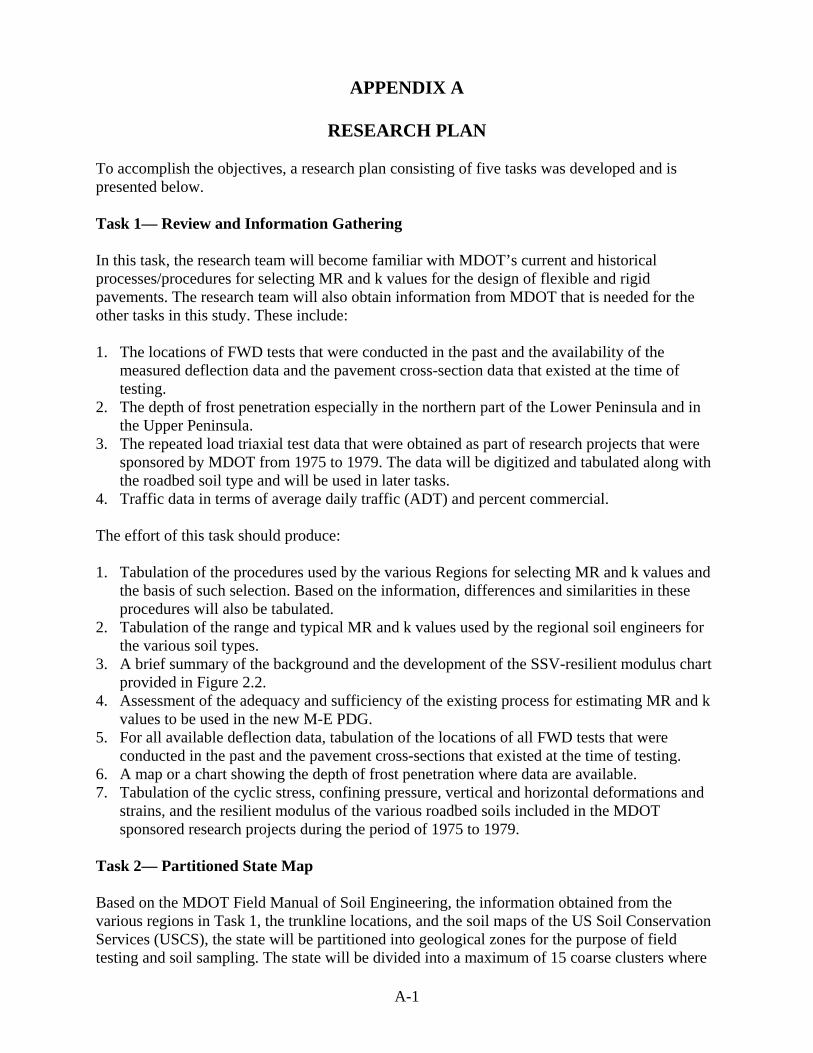
A-1 APPENDIX A RESEARCH PLAN To accomplish the objectives, a research plan consisting of five tasks was developed and is presented below. Task 1— Review and Information Gathering In this task, the research team will become familiar with MDOT’s current and historical processes/procedures for selecting MR and k values for the design of flexible and rigid pavements. The research team will also obtain information from MDOT that is needed for the other tasks in this study. These include: 1. The locations of FWD tests that were conducted in the past and the availability of the measured deflection data and the pavement cross-section data that existed at the time of testing. 2. The depth of frost penetration especially in the northern part of the Lower Peninsula and in the Upper Peninsula. 3. The repeated load triaxial test data that were obtained as part of research projects that were sponsored by MDOT from 1975 to 1979. The data will be digitized and tabulated along with the roadbed soil type and will be used in later tasks. 4. Traffic data in terms of average daily traffic (ADT) and percent commercial. The effort of this task should produce: 1. Tabulation of the procedures used by the various Regions for selecting MR and k values and the basis of such selection. Based on the information, differences and similarities in these procedures will also be tabulated. 2. Tabulation of the range and typical MR and k values used by the regional soil engineers for the various soil types. 3. A brief summary of the background and the development of the SSV-resilient modulus chart provided in Figure 2.2. 4. Assessment of the adequacy and sufficiency of the existing process for estimating MR and k values to be used in the new M-E PDG. 5. For all available deflection data, tabulation of the locations of all FWD tests that were conducted in the past and the pavement cross-sections that existed at the time of testing. 6. A map or a chart showing the depth of frost penetration where data are available. 7. Tabulation of the cyclic stress, confining pressure, vertical and horizontal deformations and strains, and the resilient modulus of the various roadbed soils included in the MDOT sponsored research projects during the period of 1975 to 1979. Task 2— Partitioned State Map Based on the MDOT Field Manual of Soil Engineering, the information obtained from the various regions in Task 1, the trunkline locations, and the soil maps of the US Soil Conservation Services (USCS), the state will be partitioned into geological zones for the purpose of field testing and soil sampling. The state will be divided into a maximum of 15 coarse clusters where
Transcript of APPENDIX A RESEARCH PLAN - michigan.gov · • The reported correlations between MR values and the...
A-1
APPENDIX A
RESEARCH PLAN
To accomplish the objectives, a research plan consisting of five tasks was developed and is presented below. Task 1— Review and Information Gathering In this task, the research team will become familiar with MDOT’s current and historical processes/procedures for selecting MR and k values for the design of flexible and rigid pavements. The research team will also obtain information from MDOT that is needed for the other tasks in this study. These include: 1. The locations of FWD tests that were conducted in the past and the availability of the
measured deflection data and the pavement cross-section data that existed at the time of testing.
2. The depth of frost penetration especially in the northern part of the Lower Peninsula and in the Upper Peninsula.
3. The repeated load triaxial test data that were obtained as part of research projects that were sponsored by MDOT from 1975 to 1979. The data will be digitized and tabulated along with the roadbed soil type and will be used in later tasks.
4. Traffic data in terms of average daily traffic (ADT) and percent commercial. The effort of this task should produce: 1. Tabulation of the procedures used by the various Regions for selecting MR and k values and
the basis of such selection. Based on the information, differences and similarities in these procedures will also be tabulated.
2. Tabulation of the range and typical MR and k values used by the regional soil engineers for the various soil types.
3. A brief summary of the background and the development of the SSV-resilient modulus chart provided in Figure 2.2.
4. Assessment of the adequacy and sufficiency of the existing process for estimating MR and k values to be used in the new M-E PDG.
5. For all available deflection data, tabulation of the locations of all FWD tests that were conducted in the past and the pavement cross-sections that existed at the time of testing.
6. A map or a chart showing the depth of frost penetration where data are available. 7. Tabulation of the cyclic stress, confining pressure, vertical and horizontal deformations and
strains, and the resilient modulus of the various roadbed soils included in the MDOT sponsored research projects during the period of 1975 to 1979.
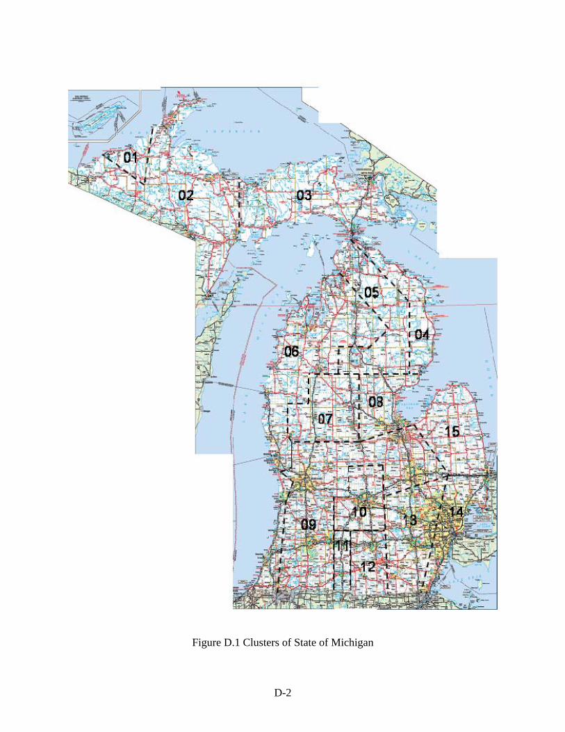
Task 2— Partitioned State Map Based on the MDOT Field Manual of Soil Engineering, the information obtained from the various regions in Task 1, the trunkline locations, and the soil maps of the US Soil Conservation Services (USCS), the state will be partitioned into geological zones for the purpose of field testing and soil sampling. The state will be divided into a maximum of 15 coarse clusters where
A-2
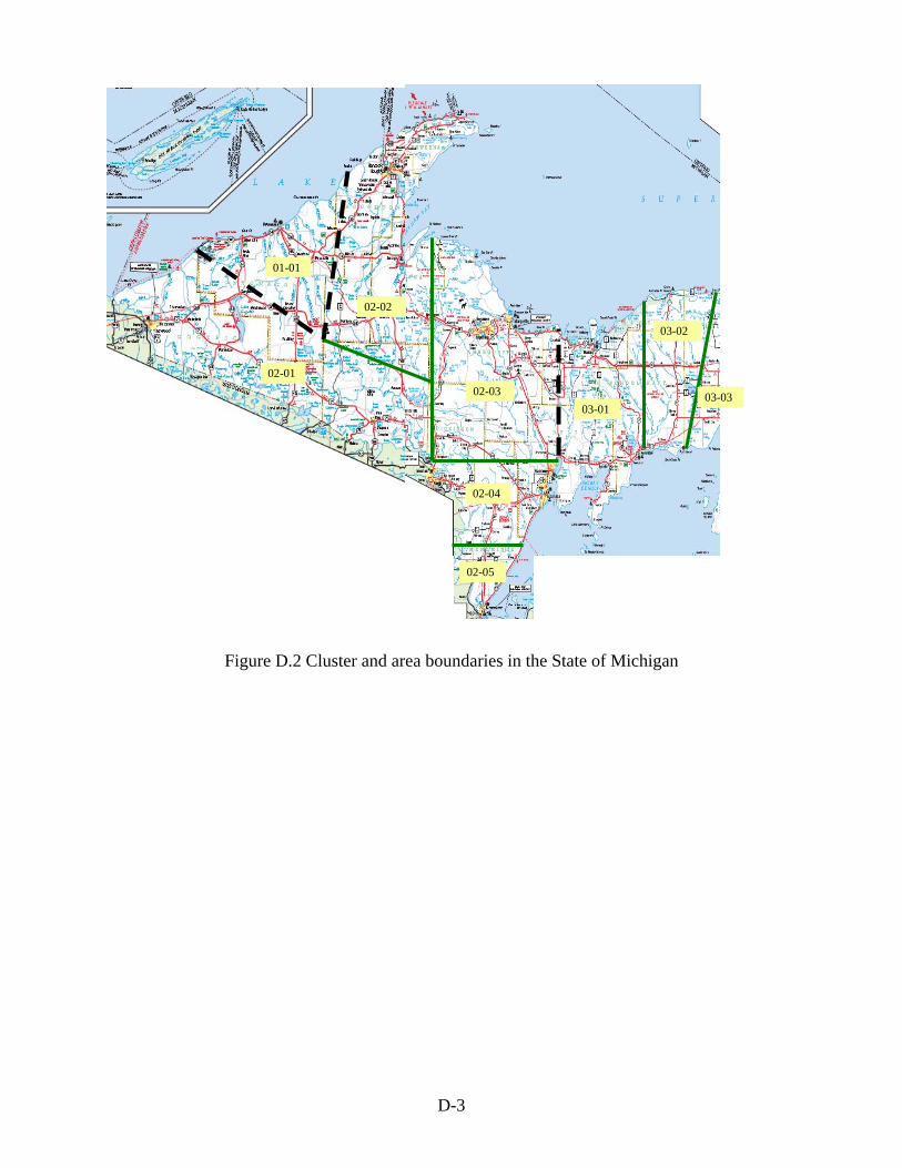
the soil within any given cluster would have similar range of engineering and physical characteristics. Each coarse cluster will then be divided into areas to narrow the range of the soil characteristics. A maximum of 99 areas will be produced. The results will be presented to members of the Research Advisory Panel (RAP) for review and possible modification. The main use of the partitioned soil map is to determine the locations of field testing and soil sampling. Task 3— Field and Laboratory Testing and Soil Sampling In this task, the research team will finalize the field sampling and the laboratory testing plans based upon the information obtained in Tasks 1 and 2. The total number of tests to be conducted will be based purely on cost and available budget. The field sampling and the laboratory testing plans are presented in three subtasks below. Subtask 3.1 - Soil Sampling Plan From each area on the State Partitioned map, soil samples will be obtained. In areas where the roadbed soil is predominantly sand, only disturbed bag samples will be collected. In clay areas, both disturbed and undisturbed thin Shelby tube samples will be obtained. In total, 75 disturbed roadbed soil samples and 12 undisturbed (Shelby tube) samples will be collected. All samples will be transported to the laboratory for testing as presented in Subtask 3.2 below. Subtask 3.2 – Laboratory Testing Plan The laboratory plan consists of moisture content, sieve, Atterberg limits, and cyclic load triaxial tests. All tests will be conducted according to MDOT, AASHTO, or ASTM standard test procedures. Results of the laboratory testing will be analyzed (see Task 4) to determine: 1. Soil classification - For each of the 75 disturbed samples (bag samples), the soil will be
subjected to sieve analyses to determine the breakdown between sand and clay/silt particles. Any sample where the fine fraction (passing sieve number 200) is more than seven percent, plastic and liquid limit tests will also be conducted. Results of the sieve analyses and Atterberg limit tests will be used to:
• Classify the soil according to the USCS and the AASHTO soil classification systems. • Develop, if possible, statistical correlations between the resilient modulus of the roadbed
soils and the gradation and Atterberg limits of the material. 2. Cyclic load triaxial tests - For each location where Shelby tubes are collected, repeated load
triaxial tests will be conducted. The samples will be tested at three moisture contents to simulate the effects of seasonal changes on the resilient modulus of the soils. The water content of the samples will be changed to the desired level by either drying or by using back pressure technique in the triaxial cell. For sand roadbed soils, the test specimens will be compacted at three moisture contents and subjected to cyclic load triaxial tests. Since the resilient moduli values of sand roadbed soils are heavily dependent upon the deviatoric stress; the laboratory tests will be conducted at three stress states which will be estimated through mechanistic analyses to simulate the probable in-situ field conditions.
A-3
Subtask 3.3 –Field Test Plan This plan consists of Falling Weight Deflectometer (FWD) tests. The FWD tests will be conducted at the network- and project-levels. At the network level, one FWD tests will be conducted at 500 foot intervals along the state trunkline. At the project level, 20 FWD tests will be conducted within + 50 ft from all locations where Shelby tubes (undisturbed soil samples) will be extracted. All FWD tests will be conducted in the spring and in the late summer – early fall seasons. For those areas where FWD tests were conducted in the past and the deflection and pavement cross-section data are available at MDOT, the data will be used and the number of FWD tests (to be conducted in those areas in this study) will be reduced depending on the availability of spring and fall deflection data. It should be noted that analyses of various damage models including AASHTO indicate that the two point FWD testing (spring and fall seasons) is adequate to assess the relative pavement damage caused by the roadbed soil due to different degrees of saturation. Task 4 – Data Analyses The data analysis, in this study, will be accomplished according to the three subtasks presented below. First, it should be noted that for all soil types, the relationship between the MR and k found in the M-E PDG was used. Since the relationship applies to all MR and k values, the analyses stated in the subtasks below will be conducted on the MR values and the results will be converted to k values. Subtask 4.1 – Backcalculation of Layer Moduli All deflection data, whether collected during this study or other studies, will be used (depending on the availability of the pavement cross-section data) to backcalculate the layer moduli using the MICHBACK computer program. Although the moduli of all pavement layers will be backcalculated, only the resilient modulus of the roadbed soils will be subjected to further analyses. The moduli of the pavement layers will be reported without further analyses. For each test area on the partition map, two sets of moduli will be backcalculated; one set will be based on the spring deflection data and the other on the late summer - early fall data. The two sets will be further analyzed to estimate the seasonal damage factor as presented in task five below. Subtask 4.2 – Laboratory Test Data Results of the cyclic load tests conducted on Shelby tube and reconstituted bag samples at three moisture contents will be analyzed to determine the laboratory values of the resilient modulus of the roadbed soil. Results of the analyses will be used to assess the impact of moisture (season) on pavement damage and to compare the values to those obtained from backcalculation. In addition, the digitized cyclic stress-strain data of those research studies that were sponsored by MDOT from 1975 to 1979 will be analyzed. This pool of information will be used as a supplement to verify the relationships or to increase the pool of data to develop more accurate relationships. The Atterberg limits (liquid limit, plastic limit, and plasticity index) and sieve analysis data will be used to classify the soil and to develop correlations to MR whenever
A-4
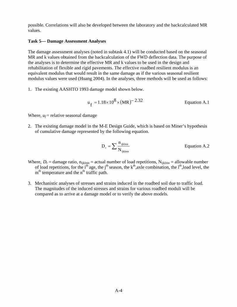
possible. Correlations will also be developed between the laboratory and the backcalculated MR values. Task 5— Damage Assessment Analyses The damage assessment analyses (noted in subtask 4.1) will be conducted based on the seasonal MR and k values obtained from the backcalculation of the FWD deflection data. The purpose of the analyses is to determine the effective MR and k values to be used in the design and rehabilitation of flexible and rigid pavements. The effective roadbed resilient modulus is an equivalent modulus that would result in the same damage as if the various seasonal resilient modulus values were used (Huang 2004). In the analyses, three methods will be used as follows: 1. The existing AASHTO 1993 damage model shown below.
( ) 2.32MR8101.18fu −××= Equation A.1
Where, uf = relative seasonal damage 2. The existing damage model in the M-E Design Guide, which is based on Miner’s hypothesis
of cumulative damage represented by the following equation.
∑=ijklmn
ijklmnr N
nD Equation A.2
Where, Dr = damage ratio, nijklmn = actual number of load repetitions, Nijklmn = allowable number
of load repetitions, for the ith age, the jth season, the kth,axle combination, the lth,load level, the mth temperature and the nth traffic path.
3. Mechanistic analyses of stresses and strains induced in the roadbed soil due to traffic load.
The magnitudes of the induced stresses and strains for various roadbed moduli will be compared as to arrive at a damage model or to verify the above models.
B-1
APPENDIX B
LITERATURE REVIEW Early in this study, an extensive literature review was conducted to study and summarize the results reported by previous investigators regarding: • The advantages and shortcomings of the laboratory and field test procedures used to
determine the MR values of roadbed soils. • The relationships between the laboratory determined and the backcalculated resilient
modulus using deflection data. • The resilient characteristics of various types of roadbed soils. • The factors affecting the MR values of roadbed soils including moisture content (seasonal
effects), particle size, Atterberg limits, and grain size distribution. • The reported correlations between MR values and the modulus of subgrade reaction (k) of
roadbed soils. • The reported correlations, if any, between the results of simple tests such as Atterberg Limits,
grain size distribution, pocket penetrometer, and hand held shear vane and the MR values of the roadbed soils.
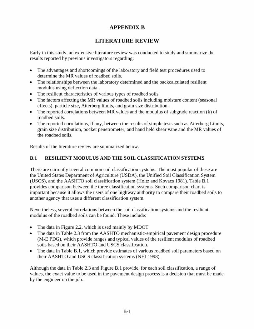
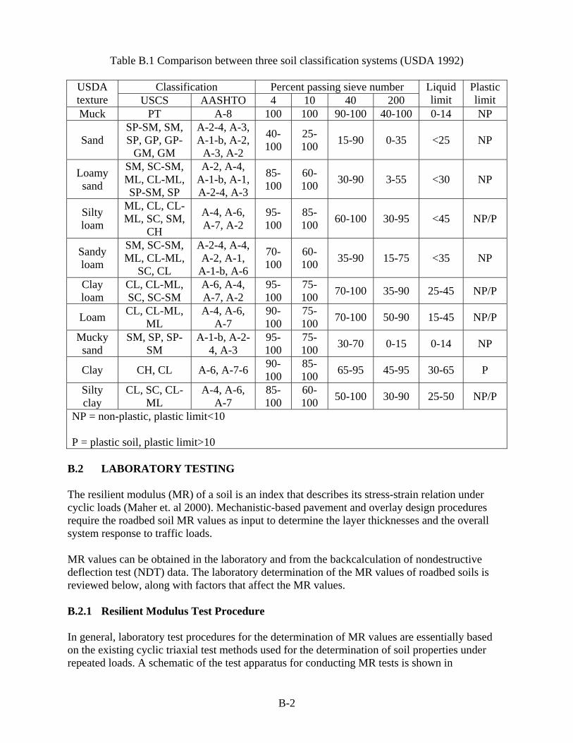
Results of the literature review are summarized below. B.1 RESILIENT MODULUS AND THE SOIL CLASSIFICATION SYSTEMS There are currently several common soil classification systems. The most popular of these are the United States Department of Agriculture (USDA), the Unified Soil Classification System (USCS), and the AASHTO soil classification system (Holtz and Kovacs 1981). Table B.1 provides comparison between the three classification systems. Such comparison chart is important because it allows the users of one highway authority to compare their roadbed soils to another agency that uses a different classification system. Nevertheless, several correlations between the soil classification systems and the resilient modulus of the roadbed soils can be found. These include: • The data in Figure 2.2, which is used mainly by MDOT. • The data in Table 2.3 from the AASHTO mechanistic-empirical pavement design procedure
(M-E PDG), which provide ranges and typical values of the resilient modulus of roadbed soils based on their AASHTO and USCS classification.
• The data in Table B.1, which provide estimates of various roadbed soil parameters based on their AASHTO and USCS classification systems (NHI 1998).
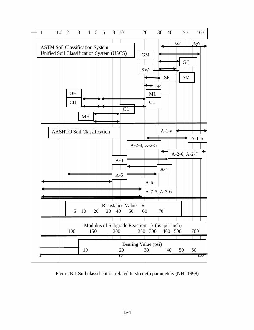
Although the data in Table 2.3 and Figure B.1 provide, for each soil classification, a range of values, the exact value to be used in the pavement design process is a decision that must be made by the engineer on the job.
B-2
Table B.1 Comparison between three soil classification systems (USDA 1992)
Classification Percent passing sieve number USDA texture USCS AASHTO 4 10 40 200
Liquid limit
Plastic limit
Muck PT A-8 100 100 90-100 40-100 0-14 NP
Sand SP-SM, SM, SP, GP, GP-
GM, GM
A-2-4, A-3, A-1-b, A-2,
A-3, A-2
40-100
25-100 15-90 0-35 <25 NP
Loamy sand
SM, SC-SM, ML, CL-ML, SP-SM, SP
A-2, A-4, A-1-b, A-1, A-2-4, A-3
85-100
60-100 30-90 3-55 <30 NP
Silty loam
ML, CL, CL-ML, SC, SM,
CH
A-4, A-6, A-7, A-2
95-100
85-100 60-100 30-95 <45 NP/P
Sandy loam
SM, SC-SM, ML, CL-ML,
SC, CL
A-2-4, A-4, A-2, A-1,
A-1-b, A-6
70-100
60-100 35-90 15-75 <35 NP
Clay loam
CL, CL-ML, SC, SC-SM
A-6, A-4, A-7, A-2
95-100
75-100 70-100 35-90 25-45 NP/P
Loam CL, CL-ML, ML
A-4, A-6, A-7
90-100
75-100 70-100 50-90 15-45 NP/P
Mucky sand
SM, SP, SP-SM
A-1-b, A-2-4, A-3
95-100
75-100 30-70 0-15 0-14 NP
Clay CH, CL A-6, A-7-6 90-100
85-100 65-95 45-95 30-65 P
Silty clay
CL, SC, CL-ML
A-4, A-6, A-7
85-100
60-100 50-100 30-90 25-50 NP/P
NP = non-plastic, plastic limit<10 P = plastic soil, plastic limit>10
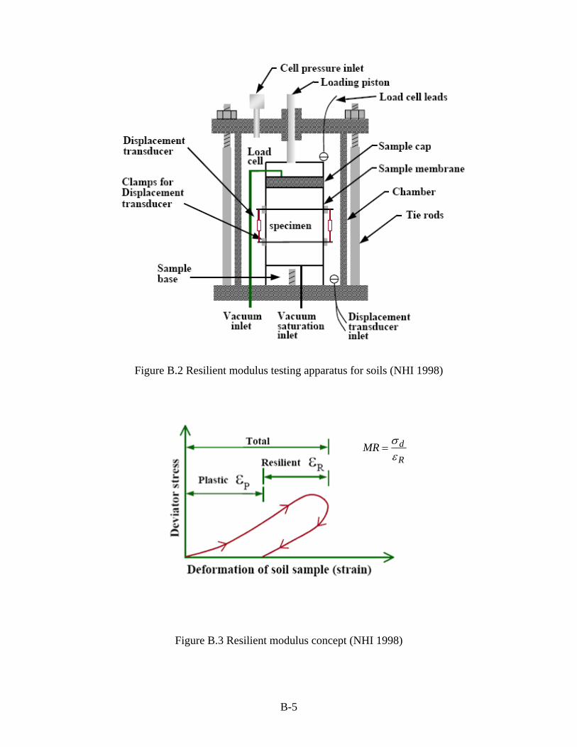
B.2 LABORATORY TESTING The resilient modulus (MR) of a soil is an index that describes its stress-strain relation under cyclic loads (Maher et. al 2000). Mechanistic-based pavement and overlay design procedures require the roadbed soil MR values as input to determine the layer thicknesses and the overall system response to traffic loads. MR values can be obtained in the laboratory and from the backcalculation of nondestructive deflection test (NDT) data. The laboratory determination of the MR values of roadbed soils is reviewed below, along with factors that affect the MR values. B.2.1 Resilient Modulus Test Procedure In general, laboratory test procedures for the determination of MR values are essentially based on the existing cyclic triaxial test methods used for the determination of soil properties under repeated loads. A schematic of the test apparatus for conducting MR tests is shown in

B-3
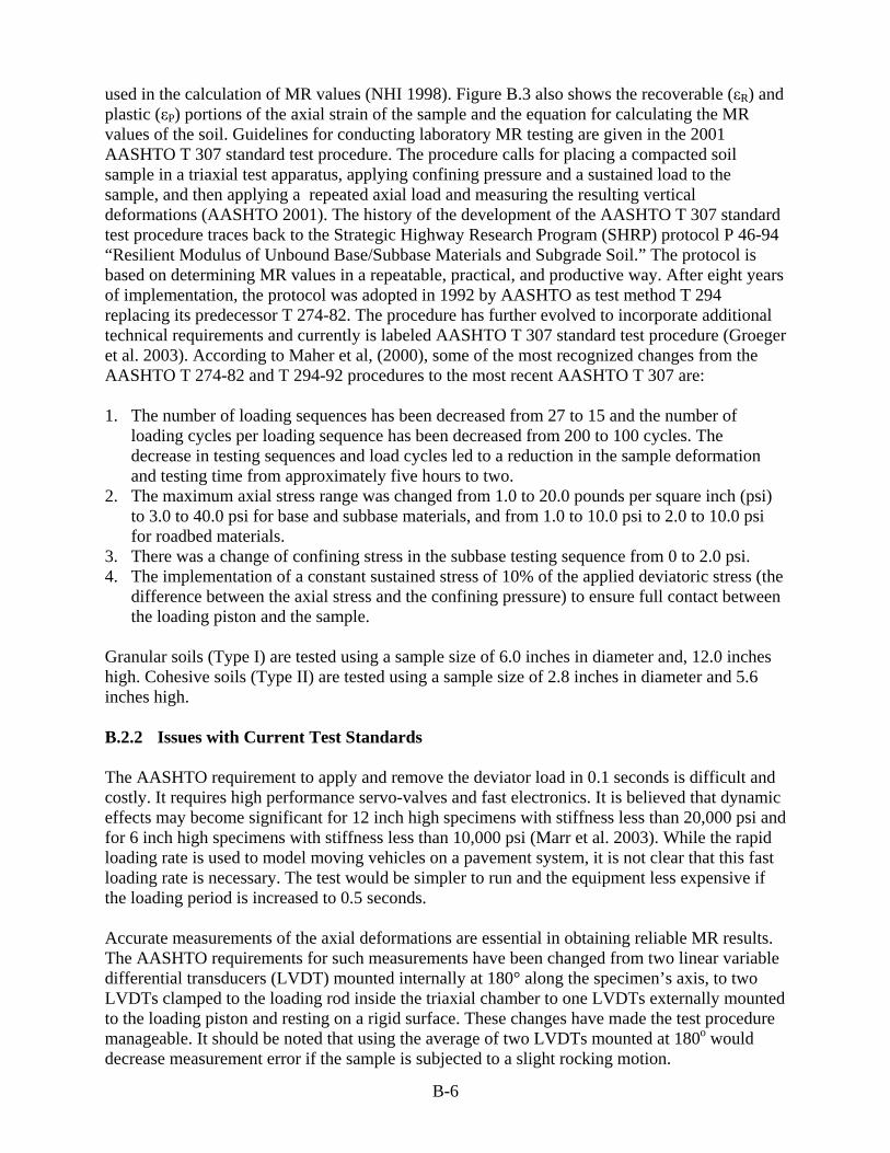
Figure B.2. Figure B.3 shows a typical hysteresis loop output (stress-strain of one load unload cycle)
B-4
Figure B.1 Soil classification related to strength parameters (NHI 1998)
0
1
1 10 100
1 1.5 2 3 4 5 6 8 10 20 30 40 70 100
GW GP
GM
Bearing Value (psi) 10 20 30 40 50 60
Modulus of Subgrade Reaction – k (psi per inch) 100 150 200 250 300 400 500 700
Resistance Value – R 5 10 20 30 40 50 60 70
AASHTO Soil Classification
ASTM Soil Classification System Unified Soil Classification System (USCS)
GC SW
SM SP
SC ML
CH OL
MH
OH
CL
A-6
A-7-5, A-7-6
A-5 A-4
A-3A-2-6, A-2-7
A-2-4, A-2-5
A-1-a A-1-b
B-5
Figure B.2 Resilient modulus testing apparatus for soils (NHI 1998)
Figure B.3 Resilient modulus concept (NHI 1998)
R
dMRεσ
=
B-6
used in the calculation of MR values (NHI 1998). Figure B.3 also shows the recoverable (εR) and plastic (εP) portions of the axial strain of the sample and the equation for calculating the MR values of the soil. Guidelines for conducting laboratory MR testing are given in the 2001 AASHTO T 307 standard test procedure. The procedure calls for placing a compacted soil sample in a triaxial test apparatus, applying confining pressure and a sustained load to the sample, and then applying a repeated axial load and measuring the resulting vertical deformations (AASHTO 2001). The history of the development of the AASHTO T 307 standard test procedure traces back to the Strategic Highway Research Program (SHRP) protocol P 46-94 “Resilient Modulus of Unbound Base/Subbase Materials and Subgrade Soil.” The protocol is based on determining MR values in a repeatable, practical, and productive way. After eight years of implementation, the protocol was adopted in 1992 by AASHTO as test method T 294 replacing its predecessor T 274-82. The procedure has further evolved to incorporate additional technical requirements and currently is labeled AASHTO T 307 standard test procedure (Groeger et al. 2003). According to Maher et al, (2000), some of the most recognized changes from the AASHTO T 274-82 and T 294-92 procedures to the most recent AASHTO T 307 are: 1. The number of loading sequences has been decreased from 27 to 15 and the number of
loading cycles per loading sequence has been decreased from 200 to 100 cycles. The decrease in testing sequences and load cycles led to a reduction in the sample deformation and testing time from approximately five hours to two.
2. The maximum axial stress range was changed from 1.0 to 20.0 pounds per square inch (psi) to 3.0 to 40.0 psi for base and subbase materials, and from 1.0 to 10.0 psi to 2.0 to 10.0 psi for roadbed materials.
3. There was a change of confining stress in the subbase testing sequence from 0 to 2.0 psi. 4. The implementation of a constant sustained stress of 10% of the applied deviatoric stress (the
difference between the axial stress and the confining pressure) to ensure full contact between the loading piston and the sample.
Granular soils (Type I) are tested using a sample size of 6.0 inches in diameter and, 12.0 inches high. Cohesive soils (Type II) are tested using a sample size of 2.8 inches in diameter and 5.6 inches high. B.2.2 Issues with Current Test Standards The AASHTO requirement to apply and remove the deviator load in 0.1 seconds is difficult and costly. It requires high performance servo-valves and fast electronics. It is believed that dynamic effects may become significant for 12 inch high specimens with stiffness less than 20,000 psi and for 6 inch high specimens with stiffness less than 10,000 psi (Marr et al. 2003). While the rapid loading rate is used to model moving vehicles on a pavement system, it is not clear that this fast loading rate is necessary. The test would be simpler to run and the equipment less expensive if the loading period is increased to 0.5 seconds. Accurate measurements of the axial deformations are essential in obtaining reliable MR results. The AASHTO requirements for such measurements have been changed from two linear variable differential transducers (LVDT) mounted internally at 180° along the specimen’s axis, to two LVDTs clamped to the loading rod inside the triaxial chamber to one LVDTs externally mounted to the loading piston and resting on a rigid surface. These changes have made the test procedure manageable. It should be noted that using the average of two LVDTs mounted at 180o would decrease measurement error if the sample is subjected to a slight rocking motion.
B-7
B.3 FIELD TESTING Field testing for determining or estimating the MR values is divided into two categories; destructive and nondestructive. B.3.1 Destructive Testing Results from the following five destructive tests are often used to estimate MR or k values. B.3.1.1 California Bearing Ratio
The California Bearing Ratio (CBR) is the ratio between the soil’s resistance to 0.1 inch penetration of a standard piston to the resistance of a well graded and crushed stone to the same penetration. The test can be conducted in the field and the laboratory as described in the AASHTO T193 standard test procedure (AASHTO 2001). The 1993 AASHTO Pavement Design Guide uses Equation B.1 to estimate the MR from the CBR values (AASHTO 1993). It should be noted that the 1500 constant in Equation B.1 can vary from 750 to 3000 (NHI 1998).
)(1500 CBRMR = Equation B.1
Whereas the new M-E PDG recommends the use of Equation B.2 for estimating the MR value (NCHRP 2004).
( ) 64.02555 CBRMR = Equation B.2
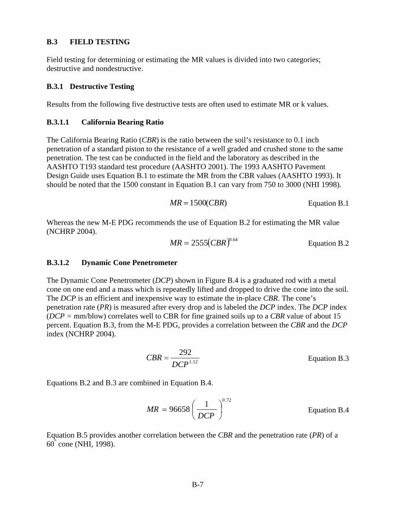
B.3.1.2 Dynamic Cone Penetrometer The Dynamic Cone Penetrometer (DCP) shown in Figure B.4 is a graduated rod with a metal cone on one end and a mass which is repeatedly lifted and dropped to drive the cone into the soil. The DCP is an efficient and inexpensive way to estimate the in-place CBR. The cone’s penetration rate (PR) is measured after every drop and is labeled the DCP index. The DCP index (DCP = mm/blow) correlates well to CBR for fine grained soils up to a CBR value of about 15 percent. Equation B.3, from the M-E PDG, provides a correlation between the CBR and the DCP index (NCHRP 2004).
12.1
292DCP
CBR = Equation B.3
Equations B.2 and B.3 are combined in Equation B.4.
72.0196658 ⎟⎠⎞
⎜⎝⎛=
DCPMR Equation B.4
Equation B.5 provides another correlation between the CBR and the penetration rate (PR) of a 60° cone (NHI, 1998).
B-8
Figure B.4 Schematic of a dynamic cone penetrometer (NHI 1998)
2591
3405.PR.CBR = Equation B.5
Where, PR = penetration rate (mm per blow)
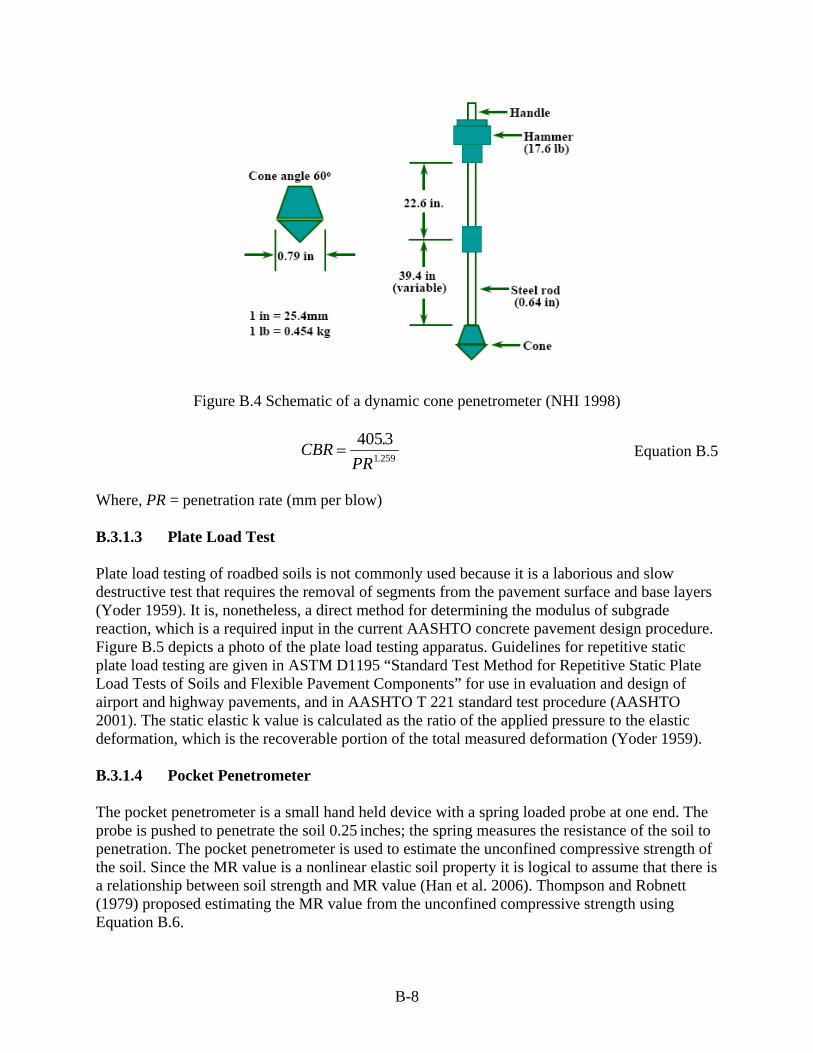
B.3.1.3 Plate Load Test Plate load testing of roadbed soils is not commonly used because it is a laborious and slow destructive test that requires the removal of segments from the pavement surface and base layers (Yoder 1959). It is, nonetheless, a direct method for determining the modulus of subgrade reaction, which is a required input in the current AASHTO concrete pavement design procedure. Figure B.5 depicts a photo of the plate load testing apparatus. Guidelines for repetitive static plate load testing are given in ASTM D1195 “Standard Test Method for Repetitive Static Plate Load Tests of Soils and Flexible Pavement Components” for use in evaluation and design of airport and highway pavements, and in AASHTO T 221 standard test procedure (AASHTO 2001). The static elastic k value is calculated as the ratio of the applied pressure to the elastic deformation, which is the recoverable portion of the total measured deformation (Yoder 1959). B.3.1.4 Pocket Penetrometer The pocket penetrometer is a small hand held device with a spring loaded probe at one end. The probe is pushed to penetrate the soil 0.25 inches; the spring measures the resistance of the soil to penetration. The pocket penetrometer is used to estimate the unconfined compressive strength of the soil. Since the MR value is a nonlinear elastic soil property it is logical to assume that there is a relationship between soil strength and MR value (Han et al. 2006). Thompson and Robnett (1979) proposed estimating the MR value from the unconfined compressive strength using Equation B.6.
B-9
Figure B.5 Photo of plate load testing apparatus (NHI 1998)
uqMR 307.86.0 += Equation B.6
Where, MR = resilient modulus (ksi) and qu = unconfined compressive strength (psi) B.3.1.5 Pocket Vane Shear Tester The pocket shear tester is used to estimate the undrained shear strength of the soil. The shear tester is inserted 0.25 inches into a flat soil surface and rotated until failure. The maximum pressure required to cause failure is the su value. Sukermaran et al (2002) suggested a relationship between the undrained shear strength and MR value.
usMR 500100 −= PI>30 Equation B.7
usMR 1500500 −= PI<30 Equation B.8
Where, MR = resilient modulus (psi), Su = undrained shear strength (psi), and PI = plasticity index
B.3.2 Nondestructive Testing Several nondestructive test procedures and equipment are being used to evaluate the engineering characteristics of roadbed soils. These include: • Ground penetrating radar (GPR) to estimate the pavement layer thicknesses • Nondestructive deflection tests (NDT) to measure the pavement response to load Literature review regarding NDT and the use of the deflection data in pavement evaluation processes are addressed in the next sections.
B-10
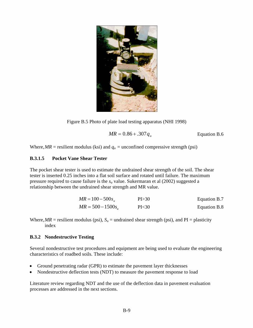
B.3.2.1 Nondestructive Deflection Tests The nondestructive deflection test (NDT) is the most popular test used in pavement evaluation. Relative to destructive testing, NDT is fast and requires minimal lane closure time. In recent years, the use of NDT has become an integral part of the structural evaluation and rehabilitation of pavement structures. The next section summarizes available NDT equipment. B.3.2.2 NDT Devices Several NDT devices have been developed. The features of each device and its advantages and disadvantages are thoroughly reviewed by Tariq Mahmood (1993), and are summarized below: • Static deflection equipment including: the Benkelman Beam, which is shown in Figure B.6,
(Moore et al 1978; Asphalt Institute 1977; Epps et al 1989), the plate bearing test (Moore et al 1978; Nazarian et al 1989), the Dehlen Curvature Meter (Gouzheng 1982), the Pavement Deflection Logging Machine (Keneddy et al 1978), and the C.E.B.T.P. Curviameter (Paquet 1978).
Figure B.6 Benkelman Beam
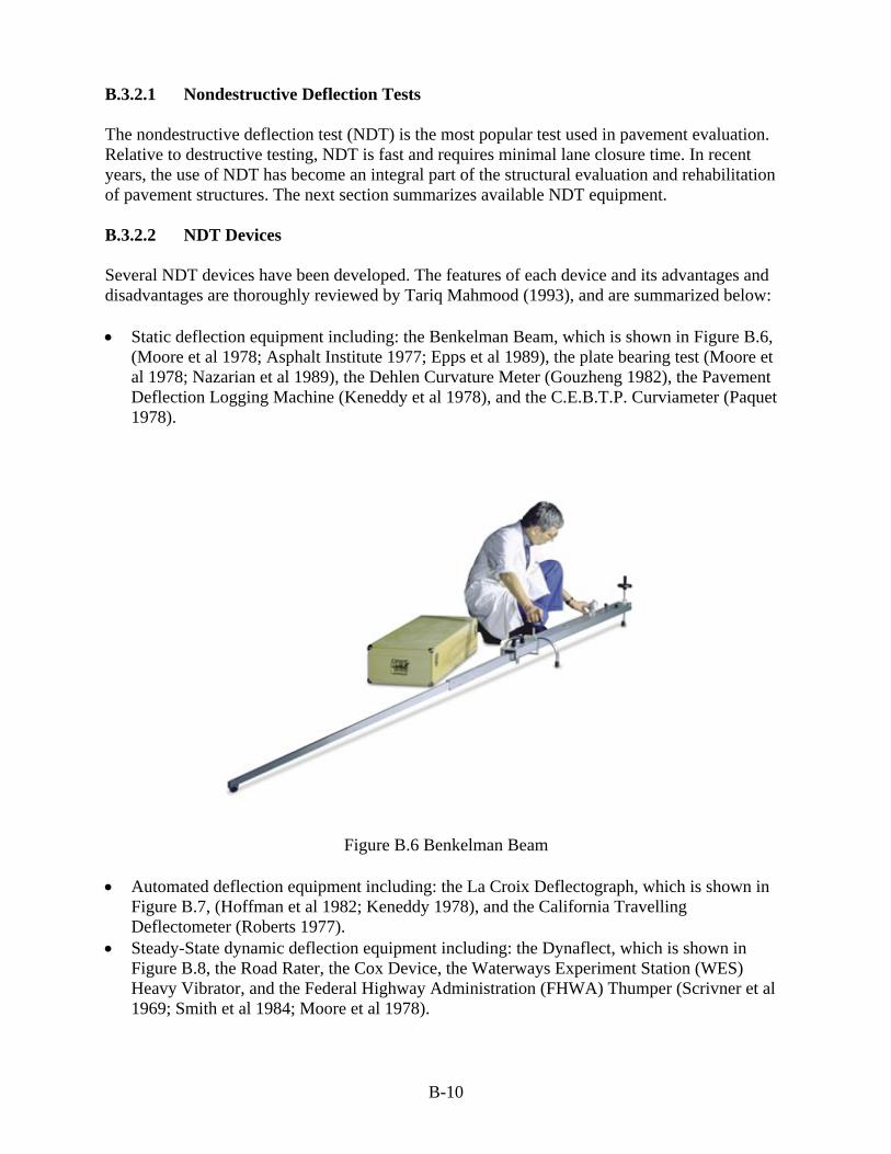
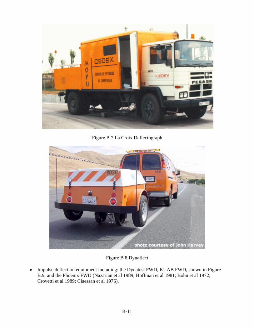
• Automated deflection equipment including: the La Croix Deflectograph, which is shown in Figure B.7, (Hoffman et al 1982; Keneddy 1978), and the California Travelling Deflectometer (Roberts 1977).
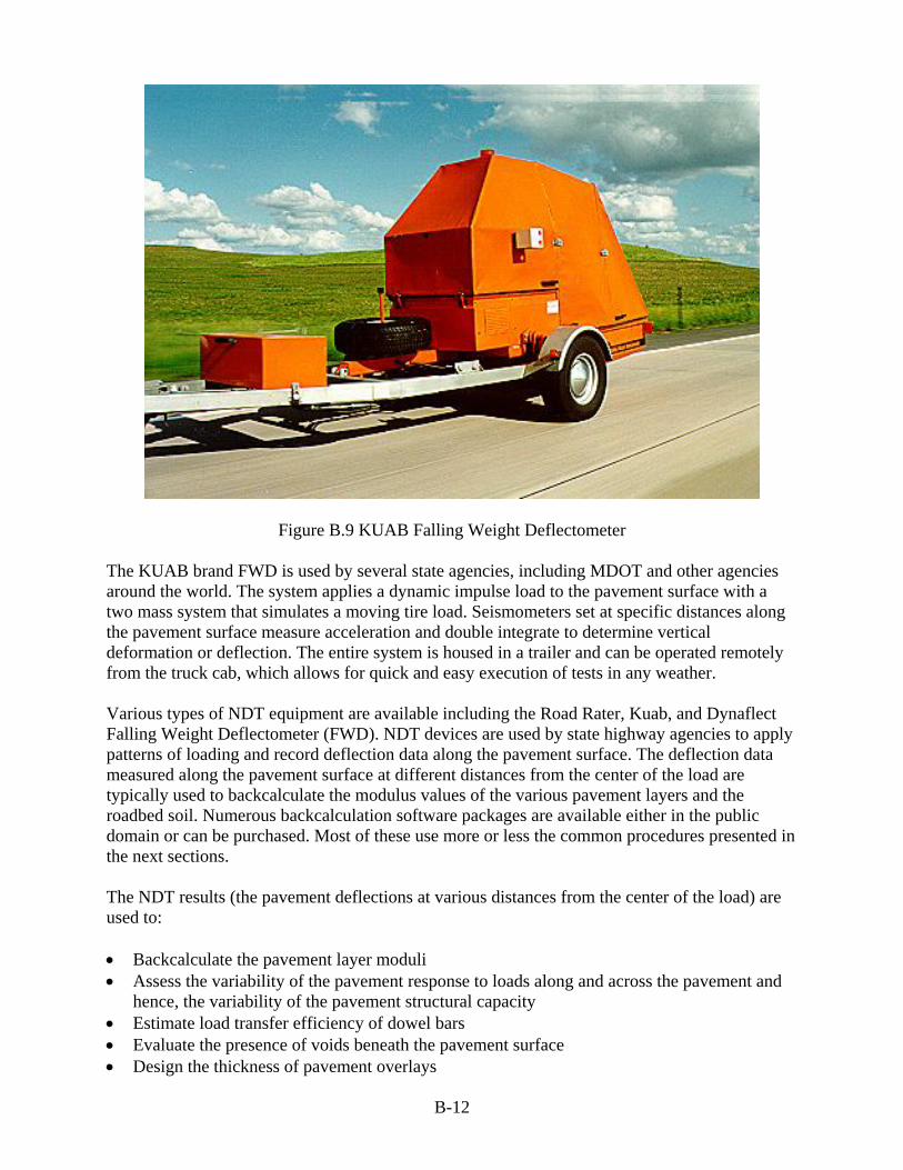
• Steady-State dynamic deflection equipment including: the Dynaflect, which is shown in Figure B.8, the Road Rater, the Cox Device, the Waterways Experiment Station (WES) Heavy Vibrator, and the Federal Highway Administration (FHWA) Thumper (Scrivner et al 1969; Smith et al 1984; Moore et al 1978).
B-11
Figure B.7 La Croix Deflectograph
Figure B.8 Dynaflect
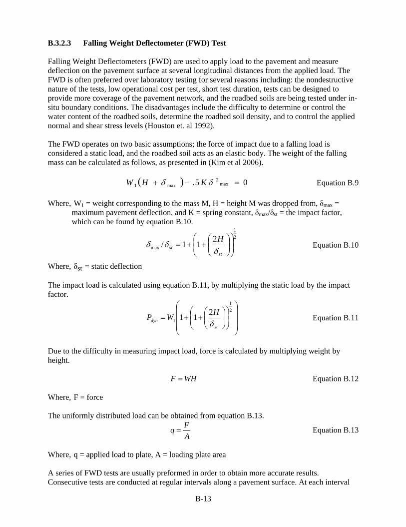
• Impulse deflection equipment including: the Dynatest FWD, KUAB FWD, shown in Figure B.9, and the Phoenix FWD (Nazarian et al 1989; Hoffman et al 1981; Bohn et al 1972; Crovetti et al 1989; Claessan et al 1976).
B-12
Figure B.9 KUAB Falling Weight Deflectometer
The KUAB brand FWD is used by several state agencies, including MDOT and other agencies around the world. The system applies a dynamic impulse load to the pavement surface with a two mass system that simulates a moving tire load. Seismometers set at specific distances along the pavement surface measure acceleration and double integrate to determine vertical deformation or deflection. The entire system is housed in a trailer and can be operated remotely from the truck cab, which allows for quick and easy execution of tests in any weather.
Various types of NDT equipment are available including the Road Rater, Kuab, and Dynaflect Falling Weight Deflectometer (FWD). NDT devices are used by state highway agencies to apply patterns of loading and record deflection data along the pavement surface. The deflection data measured along the pavement surface at different distances from the center of the load are typically used to backcalculate the modulus values of the various pavement layers and the roadbed soil. Numerous backcalculation software packages are available either in the public domain or can be purchased. Most of these use more or less the common procedures presented in the next sections. The NDT results (the pavement deflections at various distances from the center of the load) are used to: • Backcalculate the pavement layer moduli • Assess the variability of the pavement response to loads along and across the pavement and
hence, the variability of the pavement structural capacity • Estimate load transfer efficiency of dowel bars • Evaluate the presence of voids beneath the pavement surface • Design the thickness of pavement overlays
B-13
B.3.2.3 Falling Weight Deflectometer (FWD) Test
Falling Weight Deflectometers (FWD) are used to apply load to the pavement and measure deflection on the pavement surface at several longitudinal distances from the applied load. The FWD is often preferred over laboratory testing for several reasons including: the nondestructive nature of the tests, low operational cost per test, short test duration, tests can be designed to provide more coverage of the pavement network, and the roadbed soils are being tested under in-situ boundary conditions. The disadvantages include the difficulty to determine or control the water content of the roadbed soils, determine the roadbed soil density, and to control the applied normal and shear stress levels (Houston et. al 1992). The FWD operates on two basic assumptions; the force of impact due to a falling load is considered a static load, and the roadbed soil acts as an elastic body. The weight of the falling mass can be calculated as follows, as presented in (Kim et al 2006).
( ) 05. max2
max1 =−+ δδ KHW Equation B.9
Where, W1 = weight corresponding to the mass M, H = height M was dropped from, δmax = maximum pavement deflection, and K = spring constant, δmax/δst = the impact factor, which can be found by equation B.10.
21
max211/ ⎟
⎟⎠
⎞⎜⎜⎝
⎛⎟⎟⎠
⎞⎜⎜⎝
⎛++=
stst
Hδ
δδ Equation B.10
Where, δst = static deflection The impact load is calculated using equation B.11, by multiplying the static load by the impact factor.
⎟⎟⎟
⎠
⎞
⎜⎜⎜
⎝
⎛
⎟⎟⎠
⎞⎜⎜⎝
⎛⎟⎟⎠
⎞⎜⎜⎝
⎛++=
21
1211
stdyn
HWPδ
Equation B.11
Due to the difficulty in measuring impact load, force is calculated by multiplying weight by height.
WHF = Equation B.12
Where, F = force The uniformly distributed load can be obtained from equation B.13.
AFq = Equation B.13
Where, q = applied load to plate, A = loading plate area A series of FWD tests are usually preformed in order to obtain more accurate results. Consecutive tests are conducted at regular intervals along a pavement surface. At each interval

B-14
four drops of the weight are conducted. The first drop is not used in analysis, and the following three are averaged to create one set of data for each interval. This allows for average values along the pavement to be calculated. Averages are taken in order to capture the range of deflections as well as the most common values over a pavement section. The variations in deflection are due to non-constant roadbed soils and construction practices which often result in varying densities and thicknesses of the pavement layers. A typical asphalt concrete (AC) surface can range from plus or minus 1 inch of thickness from the design thickness. This can affect MR results because a constant layer thickness and Poisons’ ratio are used for the entire pavement section tested. An example of how measured deflections at each sensor vary along a pavement section is shown in Figure B.10.
0
5
10
15
20
5 15 25 35 45 55 65
Interval
Def
lect
ion
(mil)
0 inch8 inch12 inch18 inch24 inch36 inch60 inch
Figure B.10 Typical deflections at all sensors B.4 BACKCALCULATION OF LAYER MODULI OF FLEXIBLE PAVEMENT Flexible pavement layer moduli are backcalculated using deflection data from FWD tests. Deflection data is analyzed using computer programs to iteratively forward calculate deflection based on layer moduli, Poisson ratios, thicknesses, and load magnitude. Then the layer moduli are incremented until the calculated deflection is very close to the measured deflection. When the absolute or Root Mean Squared (RMS) error between the measured and calculated deflection is minimized, the results are the most accurate. There are 5 categories of assumptions that have been used to create the various computer programs; linear elastic-static, nonlinear elastic-static, linear-dynamic using frequency domain fitting, linear-dynamic using time domain fitting, and nonlinear-dynamic (Uzan 1994). Each category utilizes different assumptions and techniques. B.4.1 Backcalculation Methods for Flexible Pavement The roadbed soil modulus can be determined by using the pavement surface deflection measured at distances of 48 inch or more from the center of the load. Because of arching effects, at these
B-15
distances, the pavement surface deflection is influenced mainly by the roadbed soils. Hence, the roadbed soil MR values can be backcalculated from a single deflection measurement. The most widely used routine to backcalculate the roadbed soil MR values from a single deflection measurement is the Boussinesq equation (George 2003).
( ) ( )r
r rdCPMRor
rMRCPd
πυ
πν 22 11 −
=−
= Equation B.14
Where, dr = the surface deflection (in) at a distance r (in) from the load, P = applied load (lbs), C = correlation/adjustment factor that accounts for the difference between the backcalculated and the laboratory obtained MR value, MR = resilient modulus (psi), and ν = poison’s ratio of the asphalt layer
By assuming a Poisson’s ratio of 0.5, equation B.14 can be reduced to the following equation (AASHTO 1993).
rdCPMR
r
24.0= Equation B.15
AASHTO recommends the use of a C value of no greater than 0.33. The minimum distance (r) in Equations B.14 and B.15 is given by the following relationship.
⎟⎟⎠
⎞⎜⎜⎝
⎛×+= 3
270MRE
Da.r p Equation B.16
Where, a2 = radius of load plate (in), D = total thickness of pavement layers above the roadbed (in), andEp = effective modulus of all layers above the roadbed (psi)
Ep in equation B.16 can be calculated by using Equation B.17:
⎪⎪⎪⎪
⎭
⎪⎪⎪⎪
⎬
⎫
⎪⎪⎪⎪
⎩
⎪⎪⎪⎪
⎨
⎧
⎟⎟⎠
⎞⎜⎜⎝
⎛
⎟⎠⎞
⎜⎝⎛+
−
+
⎥⎥⎦
⎤
⎢⎢⎣
⎡+
=××
MRE
aD
MRE
aD
aqdMR
pp
o
2
2
3
1
11
1
15.1 Equation B.17
Where, do = deflection measured at the center of the load plate after adjustment to temperature of
68 oF, q = pressure on load plate (psi), D = total thickness of pavement layers above the roadbed soil (inch), and Ep = effective modulus of all layers above the roadbed soil (psi)
The Washington State Department of Transportation (WSDOT) developed, for asphalt pavements, Equations B.18 through B.20 and, for concrete pavements, Equation B.21 to estimate the roadbed soil modulus from deflection sensors located at various distances from the center of the load (Pierce 1999).
B-16
24242892.09000)(
dpsiMR = Equation B.18
36
00762.09000466)(d
psiMR +−= Equation B.19
48
00567.09000198)(d
psiMR +−= Equation B.20
And for concrete pavements,
48
00577.09000111)(d
psiMR +−= Equation B.21
Where, d24, d36, and d48 are the pavement surface deflections (mil) measured at 24, 36, and 48 inches from the center of the load
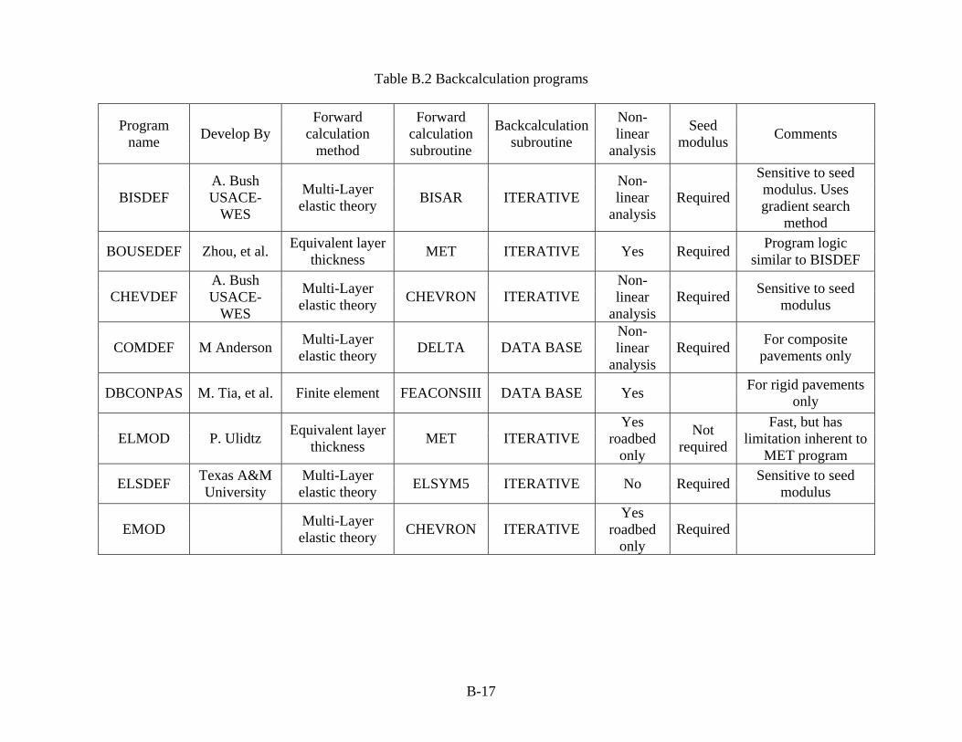
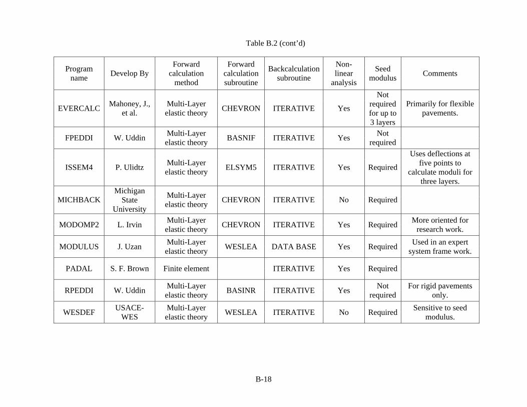
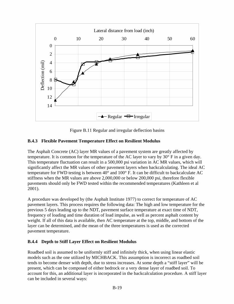
There are several different computer programs that utilize the before mentioned backcalculation methods, each with varying assumptions, routines, and methods. Table B.2 lists many of the available backcalculation programs. B.4.2 MICHBACK The program for backcalculation of layer moduli of flexible pavement used in this report is MICHBACK, developed at Michigan State University (MSU). MICHBACK uses the Chevronx (a multilayer elastic program) as the forward engine to calculate the pavement deflections for a given set of data (layer moduli and Poisson ratios, layer thicknesses, and load magnitude). The MICHBACK program utilizes a modified Newtonian algorithm to increment the layer modulus values based on differences between the measured and the backcalculated pavement deflections (George 2003). A brief summary of the MICHBACK program procedure is presented below. A detailed flow-sheet can be found in (Mahmood 1993). o Input initial data (pavement location, file name, layer information, etc...) o Upload FWD file, or manually input deflection data o Input modulus seed values and stiff layer depth o Perform backcalculation o View or print results MICHBACK uses a linear-elastic model, as mentioned previously. In order for the program to work correctly, and converge, the deflection basin must be uniform with an elastic system. The main contributing factor leading to non-convergence is the degree of irregularity of the deflection basin. For the backcalculation of layer moduli to be successful, the shape of the deflection basin must be smooth and compatible with the elastic layer theory. Highly irregular measured deflection basins (such as that shown in Figure B.11) cannot be matched to that calculated using the layer elastic theory. Irregularities in the deflection basins could be caused by an uneven contact between one or more deflection sensors and the pavement surface, debris (such as sand particles) between the deflection sensors and the pavement surface, and/or cracks or other structural distresses in the pavement that adversely impact the continuity of the stress dissipation with depth and distance from the load.
B-17
Table B.2 Backcalculation programs
Program name Develop By
Forward calculation
method
Forward calculation subroutine
Backcalculation subroutine
Non-linear
analysis
Seed modulus Comments
BISDEF A. Bush USACE-
WES
Multi-Layer elastic theory BISAR ITERATIVE
Non-linear
analysis Required
Sensitive to seed modulus. Uses gradient search
method
BOUSEDEF Zhou, et al. Equivalent layer thickness MET ITERATIVE Yes Required Program logic
similar to BISDEF
CHEVDEF A. Bush USACE-
WES
Multi-Layer elastic theory CHEVRON ITERATIVE
Non-linear
analysis Required Sensitive to seed
modulus
COMDEF M Anderson Multi-Layer elastic theory DELTA DATA BASE
Non-linear
analysis Required For composite
pavements only
DBCONPAS M. Tia, et al. Finite element FEACONSIII DATA BASE Yes For rigid pavements only
ELMOD P. Ulidtz Equivalent layer thickness MET ITERATIVE
Yes roadbed
only
Not required
Fast, but has limitation inherent to
MET program
ELSDEF Texas A&M University
Multi-Layer elastic theory ELSYM5 ITERATIVE No Required Sensitive to seed
modulus
EMOD Multi-Layer elastic theory CHEVRON ITERATIVE
Yes roadbed
only Required
B-18
Table B.2 (cont’d)
Program name Develop By
Forward calculation
method
Forward calculation subroutine
Backcalculation subroutine
Non-linear
analysis
Seed modulus Comments
EVERCALC Mahoney, J., et al.
Multi-Layer elastic theory CHEVRON ITERATIVE Yes
Not required for up to 3 layers
Primarily for flexible pavements.
FPEDDI W. Uddin Multi-Layer elastic theory BASNIF ITERATIVE Yes Not
required
ISSEM4 P. Ulidtz Multi-Layer elastic theory ELSYM5 ITERATIVE Yes Required
Uses deflections at five points to
calculate moduli for three layers.
MICHBACK Michigan
State University
Multi-Layer elastic theory CHEVRON ITERATIVE No Required
MODOMP2 L. Irvin Multi-Layer elastic theory CHEVRON ITERATIVE Yes Required More oriented for
research work.
MODULUS J. Uzan Multi-Layer elastic theory WESLEA DATA BASE Yes Required Used in an expert
system frame work.
PADAL S. F. Brown Finite element ITERATIVE Yes Required
RPEDDI W. Uddin Multi-Layer elastic theory BASINR ITERATIVE Yes Not
required For rigid pavements
only.
WESDEF USACE-WES
Multi-Layer elastic theory WESLEA ITERATIVE No Required Sensitive to seed
modulus.
B-19
0
2
4
6
8
10
12
14
0 10 20 30 40 50 60
Lateral distance from load (inch)
Def
lect
ion
(mil)
Regular Irregular
Figure B.11 Regular and irregular deflection basins
B.4.3 Flexible Pavement Temperature Effect on Resilient Modulus The Asphalt Concrete (AC) layer MR values of a pavement system are greatly affected by temperature. It is common for the temperature of the AC layer to vary by 30° F in a given day. This temperature fluctuation can result in a 500,000 psi variation in AC MR values, which will significantly affect the MR values of other pavement layers when backcalculating. The ideal AC temperature for FWD testing is between 40° and 100° F. It can be difficult to backcalculate AC stiffness when the MR values are above 2,000,000 or below 200,000 psi, therefore flexible pavements should only be FWD tested within the recommended temperatures (Kathleen et al 2001). A procedure was developed by (the Asphalt Institute 1977) to correct for temperature of AC pavement layers. This process requires the following data: The high and low temperature for the previous 5 days leading up to the NDT, pavement surface temperature at exact time of NDT, frequency of loading and time duration of load impulse, as well as percent asphalt content by weight. If all of this data is available, then AC temperature at the top, middle, and bottom of the layer can be determined, and the mean of the three temperatures is used as the corrected pavement temperature. B.4.4 Depth to Stiff Layer Effect on Resilient Modulus Roadbed soil is assumed to be uniformly stiff and infinitely thick, when using linear elastic models such as the one utilized by MICHBACK. This assumption is incorrect as roadbed soil tends to become denser with depth, due to stress increases. At some depth a “stiff layer” will be present, which can be composed of either bedrock or a very dense layer of roadbed soil. To account for this, an additional layer is incorporated in the backcalculation procedure. A stiff layer can be included in several ways:
B-20
• Assignment of a very high modulus to the lowest layer in the pavement system; however the depth to this layer will be unknown.
• Assignment of a 20 ft. depth to stiff layer for all FWD analyses (Bush 1980). • Use of measured velocity of compression waves and frequency of loading (Uddin et al 1986). • Application of trial and error method carried out until a minimum RMS error is reached
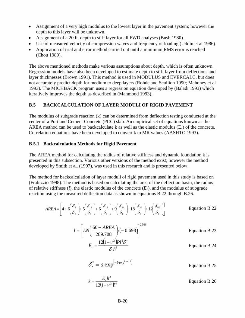
(Chou 1989). The above mentioned methods make various assumptions about depth, which is often unknown. Regression models have also been developed to estimate depth to stiff layer from deflections and layer thicknesses (Brown 1991). This method is used in MODULUS and EVERCALC, but does not accurately predict depth for medium to deep layers (Rohde and Scullion 1990; Mahoney et al 1993). The MICHBACK program uses a regression equation developed by (Baladi 1993) which iteratively improves the depth as described in (Mahmood 1993). B.5 BACKCALCULATION OF LAYER MODULI OF RIGID PAVEMENT The modulus of subgrade reaction (k) can be determined from deflection testing conducted at the center of a Portland Cement Concrete (PCC) slab. An empirical set of equations known as the AREA method can be used to backcalculate k as well as the elastic modulus (Ec) of the concrete. Correlation equations have been developed to convert k to MR values (AASHTO 1993). B.5.1 Backcalculation Methods for Rigid Pavement The AREA method for calculating the radius of relative stiffness and dynamic foundation k is presented in this subsection. Various other versions of the method exist; however the method developed by Smith et al. (1997), was used in this research and is presented below. The method for backcalculation of layer moduli of rigid pavement used in this study is based on (Frabizzio 1998). The method is based on calculating the area of the deflection basin, the radius of relative stiffness (l), the elastic modulus of the concrete (Ec), and the modulus of subgrade reaction using the measured deflection data as shown in equations B.22 through B.26.
⎥⎥⎦
⎤
⎢⎢⎣
⎡⎟⎟⎠
⎞⎜⎜⎝
⎛+⎟⎟
⎠
⎞⎜⎜⎝
⎛+⎟⎟
⎠
⎞⎜⎜⎝
⎛+⎟⎟
⎠
⎞⎜⎜⎝
⎛+⎟⎟
⎠
⎞⎜⎜⎝
⎛+⎟⎟
⎠
⎞⎜⎜⎝
⎛+=
0
60
0
36
0
24
0
18
0
12
0
8 121896564δδ
δδ
δδ
δδ
δδ
δδ
AREA Equation B.22
( )566.2
698.0/708.289
60⎥⎦
⎤⎢⎣
⎡−⎟
⎠⎞
⎜⎝⎛ −
=AREALNl Equation B.23
( )3
*22112h
PlEr
rc δ
δν−= Equation B.24
( )[ ]clb
r a−−= exp* expδ Equation B.25
( ) 42
3
112 lhEk c
ν−= Equation B.26
B-21
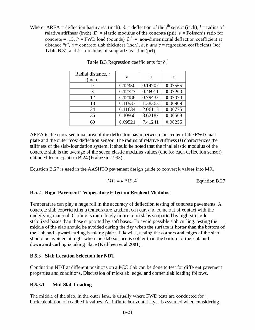
Where, AREA = deflection basin area (inch), δr = deflection of the rth sensor (inch), l = radius of relative stiffness (inch), Ec = elastic modulus of the concrete (psi), υ = Poisson’s ratio for concrete = .15, P = FWD load (pounds), δr
* = non-dimensional deflection coefficient at
distance “r”, h = concrete slab thickness (inch), a, b and c = regression coefficients (see Table B.3), and k = modulus of subgrade reaction (pci)
Table B.3 Regression coefficients for δr
*
Radial distance, r
(inch) a b c
0 0.12450 0.14707 0.07565 8 0.12323 0.46911 0.07209 12 0.12188 0.79432 0.07074 18 0.11933 1.38363 0.06909 24 0.11634 2.06115 0.06775 36 0.10960 3.62187 0.06568 60 0.09521 7.41241 0.06255
AREA is the cross-sectional area of the deflection basin between the center of the FWD load plate and the outer most deflection sensor. The radius of relative stiffness (l) characterizes the stiffness of the slab-foundation system. It should be noted that the final elastic modulus of the concrete slab is the average of the seven elastic modulus values (one for each deflection sensor) obtained from equation B.24 (Frabizzio 1998). Equation B.27 is used in the AASHTO pavement design guide to convert k values into MR.
4.19*kMR = Equation B.27 B.5.2 Rigid Pavement Temperature Effect on Resilient Modulus Temperature can play a huge roll in the accuracy of deflection testing of concrete pavements. A concrete slab experiencing a temperature gradient can curl and come out of contact with the underlying material. Curling is more likely to occur on slabs supported by high-strength stabilized bases than those supported by soft bases. To avoid possible slab curling, testing the middle of the slab should be avoided during the day when the surface is hotter than the bottom of the slab and upward curling is taking place. Likewise, testing the corners and edges of the slab should be avoided at night when the slab surface is colder than the bottom of the slab and downward curling is taking place (Kathleen et al 2001). B.5.3 Slab Location Selection for NDT Conducting NDT at different positions on a PCC slab can be done to test for different pavement properties and conditions. Discussion of mid-slab, edge, and corner slab loading follows. B.5.3.1 Mid-Slab Loading The middle of the slab, in the outer lane, is usually where FWD tests are conducted for backcalculation of roadbed k values. An infinite horizontal layer is assumed when considering
B-22
rigid pavements, due to the evenly distributed load under a loaded slab. However, the standard 12-ft highway lane width is smaller than that required for the assumption of an infinite horizontal layer, but this is often ignored. The middle of the slab is tested to create the largest distance from pavement joints and edges, and from any distresses at these locations (Kathleen et al 2001). B.5.3.2 Joint Loading Loading near the joint of a concrete slab is usually done to calculate Load Transfer Efficiency (LTE). One sensor can be placed on the loaded slab and all others on the unloaded slab. The ratio between the approach and leave slab deflection is used in calculation of LTE. The deflection measured from the 60-inch sensor can be used for roadbed MR backcalculation (Kathleen et al 2001). B.5.3.3 Edge Loading Loading the edge of a concrete slab is done to estimate the slab support to its adjacent structure, shoulder, or lane, as well as the presence of voids underneath the slab. This testing location is not normally used for backcalculation purposes. B.6 CORRELATIONS BETWEEN BACKCALCULATED MODULUS,
LABORATORY-BASED MODULUS, DCP, AND SOIL PHYSICAL PROPERTIES
Many correlations exist to convert laboratory modulus to backcalculated modulus. There are also correlations between soil properties and their MR values. An introduction to these correlations can be found below. B.6.1 Correlations between Laboratory and Backcalculated Resilient Modulus The primary purpose of establishing relationships between backcalculated FWD modulus and laboratory modulus is for the design of pavement overlays. The laboratory MR values are stress dependent. Therefore, in order to compare the different modulus values, the stress state in which the FWD test was performed must be known (George 2003). Whether the laboratory modulus or field modulus of the roadbed soil is used in the pavement design and analysis depends on the input required for the model being used. For example, the original American Association of State Highway Officials (AASHO) road test was calibrated to the laboratory MR values of the soil. Therefore, when using the 1993 AASHTO pavement design or overlay procedures, the appropriate input for the roadbed soil is the laboratory MR value (AASHTO 1993). MR values obtained from laboratory tests may be considerably lower than the backcalculated MR values due to differences in the magnitudes of the deviatoric stress, confining pressure, and loading rate (George 2003). Similarly, field MR values for fine grained soils, obtained by backcalculation from FWD deflections, have been reported in a number of studies to exceed the laboratory resilient modulus values by factors between 3 and 5 (AASHTO 1993).
B-23
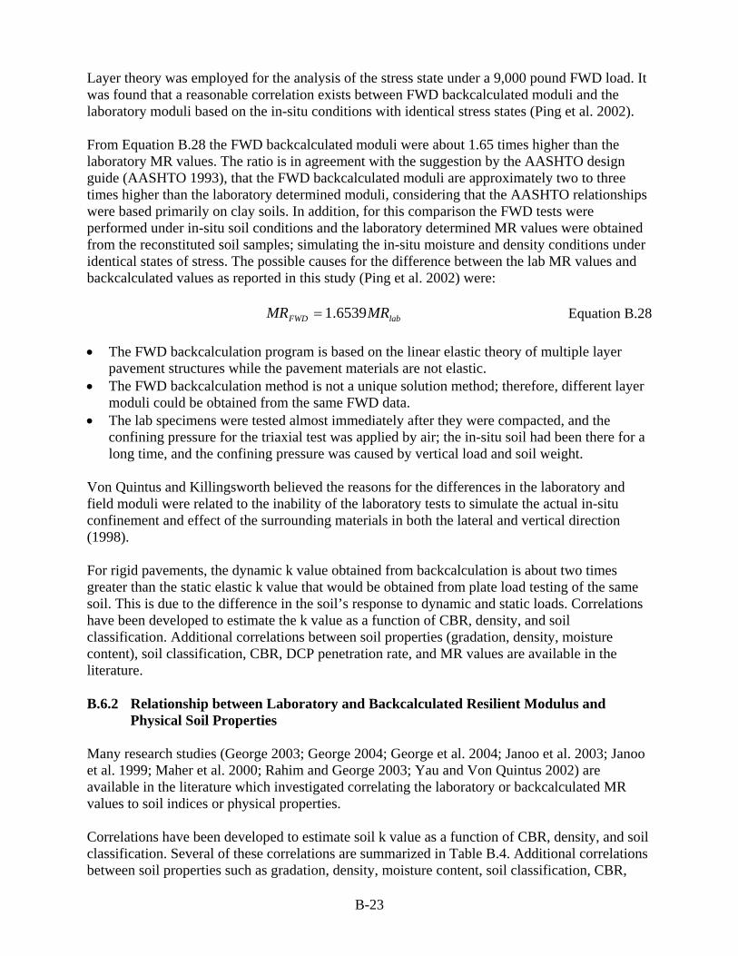
Layer theory was employed for the analysis of the stress state under a 9,000 pound FWD load. It was found that a reasonable correlation exists between FWD backcalculated moduli and the laboratory moduli based on the in-situ conditions with identical stress states (Ping et al. 2002). From Equation B.28 the FWD backcalculated moduli were about 1.65 times higher than the laboratory MR values. The ratio is in agreement with the suggestion by the AASHTO design guide (AASHTO 1993), that the FWD backcalculated moduli are approximately two to three times higher than the laboratory determined moduli, considering that the AASHTO relationships were based primarily on clay soils. In addition, for this comparison the FWD tests were performed under in-situ soil conditions and the laboratory determined MR values were obtained from the reconstituted soil samples; simulating the in-situ moisture and density conditions under identical states of stress. The possible causes for the difference between the lab MR values and backcalculated values as reported in this study (Ping et al. 2002) were:
labFWD MRMR 6539.1= Equation B.28 • The FWD backcalculation program is based on the linear elastic theory of multiple layer
pavement structures while the pavement materials are not elastic. • The FWD backcalculation method is not a unique solution method; therefore, different layer
moduli could be obtained from the same FWD data. • The lab specimens were tested almost immediately after they were compacted, and the
confining pressure for the triaxial test was applied by air; the in-situ soil had been there for a long time, and the confining pressure was caused by vertical load and soil weight.
Von Quintus and Killingsworth believed the reasons for the differences in the laboratory and field moduli were related to the inability of the laboratory tests to simulate the actual in-situ confinement and effect of the surrounding materials in both the lateral and vertical direction (1998). For rigid pavements, the dynamic k value obtained from backcalculation is about two times greater than the static elastic k value that would be obtained from plate load testing of the same soil. This is due to the difference in the soil’s response to dynamic and static loads. Correlations have been developed to estimate the k value as a function of CBR, density, and soil classification. Additional correlations between soil properties (gradation, density, moisture content), soil classification, CBR, DCP penetration rate, and MR values are available in the literature. B.6.2 Relationship between Laboratory and Backcalculated Resilient Modulus and
Physical Soil Properties Many research studies (George 2003; George 2004; George et al. 2004; Janoo et al. 2003; Janoo et al. 1999; Maher et al. 2000; Rahim and George 2003; Yau and Von Quintus 2002) are available in the literature which investigated correlating the laboratory or backcalculated MR values to soil indices or physical properties. Correlations have been developed to estimate soil k value as a function of CBR, density, and soil classification. Several of these correlations are summarized in Table B.4. Additional correlations between soil properties such as gradation, density, moisture content, soil classification, CBR,
B-24
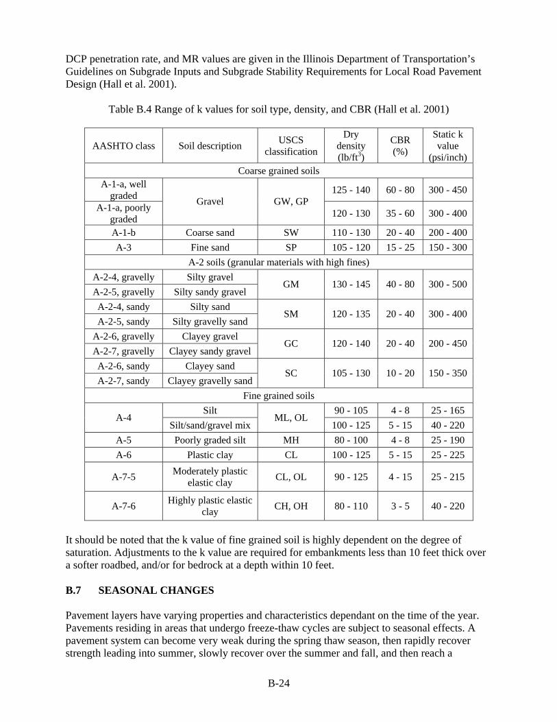
DCP penetration rate, and MR values are given in the Illinois Department of Transportation’s Guidelines on Subgrade Inputs and Subgrade Stability Requirements for Local Road Pavement Design (Hall et al. 2001).
Table B.4 Range of k values for soil type, density, and CBR (Hall et al. 2001)
AASHTO class Soil description USCS classification
Dry density (lb/ft3)
CBR (%)
Static k value
(psi/inch) Coarse grained soils
A-1-a, well graded 125 - 140 60 - 80 300 - 450
A-1-a, poorly graded
Gravel GW, GP 120 - 130 35 - 60 300 - 400
A-1-b Coarse sand SW 110 - 130 20 - 40 200 - 400 A-3 Fine sand SP 105 - 120 15 - 25 150 - 300
A-2 soils (granular materials with high fines) A-2-4, gravelly Silty gravel A-2-5, gravelly Silty sandy gravel
GM 130 - 145 40 - 80 300 - 500
A-2-4, sandy Silty sand A-2-5, sandy Silty gravelly sand
SM 120 - 135 20 - 40 300 - 400
A-2-6, gravelly Clayey gravel A-2-7, gravelly Clayey sandy gravel
GC 120 - 140 20 - 40 200 - 450
A-2-6, sandy Clayey sand A-2-7, sandy Clayey gravelly sand
SC 105 - 130 10 - 20 150 - 350
Fine grained soils Silt 90 - 105 4 - 8 25 - 165
A-4 Silt/sand/gravel mix
ML, OL 100 - 125 5 - 15 40 - 220
A-5 Poorly graded silt MH 80 - 100 4 - 8 25 - 190 A-6 Plastic clay CL 100 - 125 5 - 15 25 - 225
A-7-5 Moderately plastic elastic clay CL, OL 90 - 125 4 - 15 25 - 215
A-7-6 Highly plastic elastic clay CH, OH 80 - 110 3 - 5 40 - 220
It should be noted that the k value of fine grained soil is highly dependent on the degree of saturation. Adjustments to the k value are required for embankments less than 10 feet thick over a softer roadbed, and/or for bedrock at a depth within 10 feet. B.7 SEASONAL CHANGES Pavement layers have varying properties and characteristics dependant on the time of the year. Pavements residing in areas that undergo freeze-thaw cycles are subject to seasonal effects. A pavement system can become very weak during the spring thaw season, then rapidly recover strength leading into summer, slowly recover over the summer and fall, and then reach a
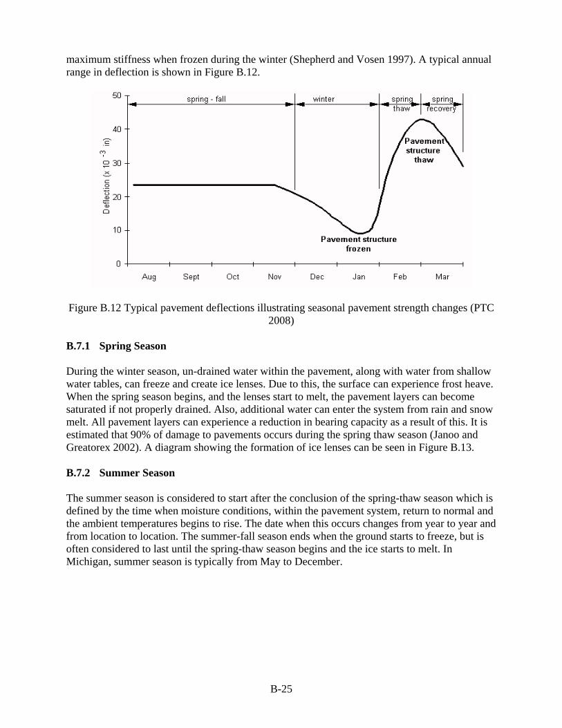
B-25
maximum stiffness when frozen during the winter (Shepherd and Vosen 1997). A typical annual range in deflection is shown in Figure B.12.
Figure B.12 Typical pavement deflections illustrating seasonal pavement strength changes (PTC 2008)
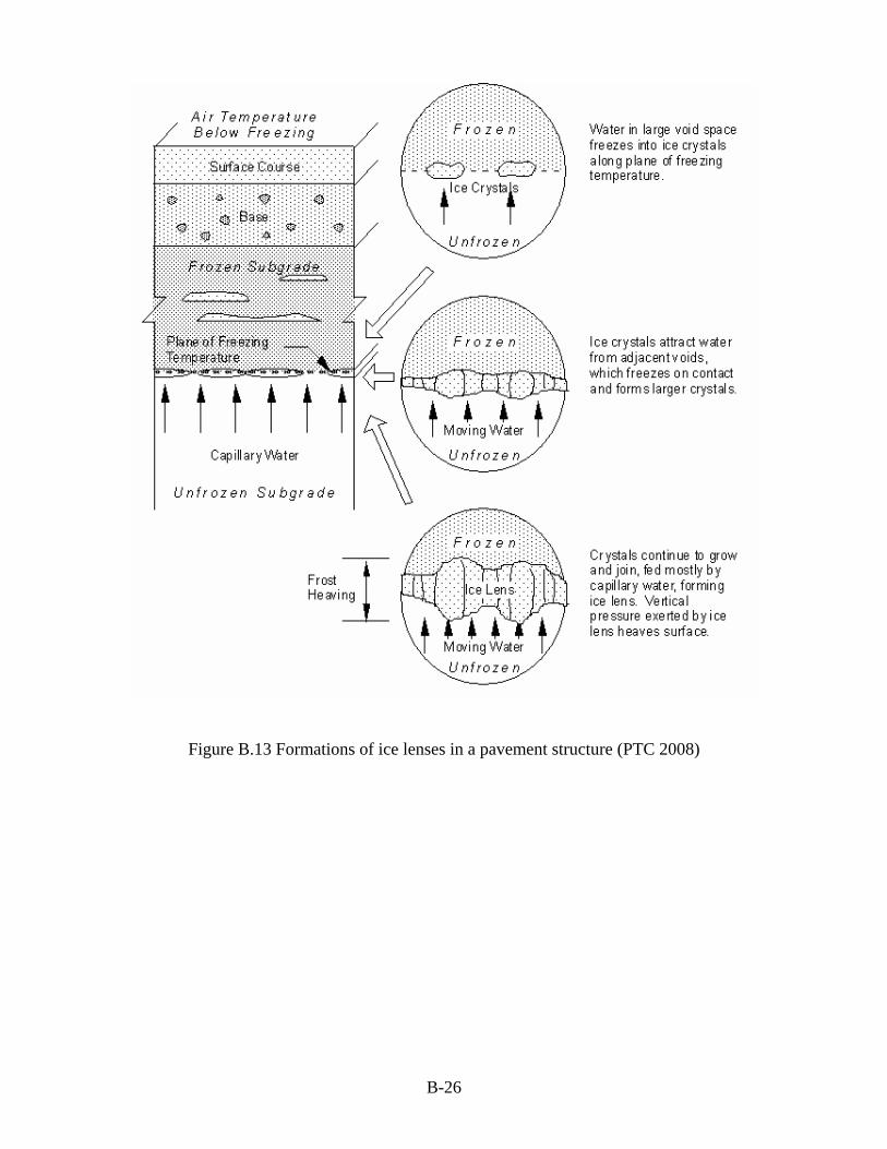
B.7.1 Spring Season During the winter season, un-drained water within the pavement, along with water from shallow water tables, can freeze and create ice lenses. Due to this, the surface can experience frost heave. When the spring season begins, and the lenses start to melt, the pavement layers can become saturated if not properly drained. Also, additional water can enter the system from rain and snow melt. All pavement layers can experience a reduction in bearing capacity as a result of this. It is estimated that 90% of damage to pavements occurs during the spring thaw season (Janoo and Greatorex 2002). A diagram showing the formation of ice lenses can be seen in Figure B.13. B.7.2 Summer Season The summer season is considered to start after the conclusion of the spring-thaw season which is defined by the time when moisture conditions, within the pavement system, return to normal and the ambient temperatures begins to rise. The date when this occurs changes from year to year and from location to location. The summer-fall season ends when the ground starts to freeze, but is often considered to last until the spring-thaw season begins and the ice starts to melt. In Michigan, summer season is typically from May to December.
B-26
Figure B.13 Formations of ice lenses in a pavement structure (PTC 2008)
C-1
APPENDIX C
SOIL CLASSIFICATION SYSTEMS
C-2
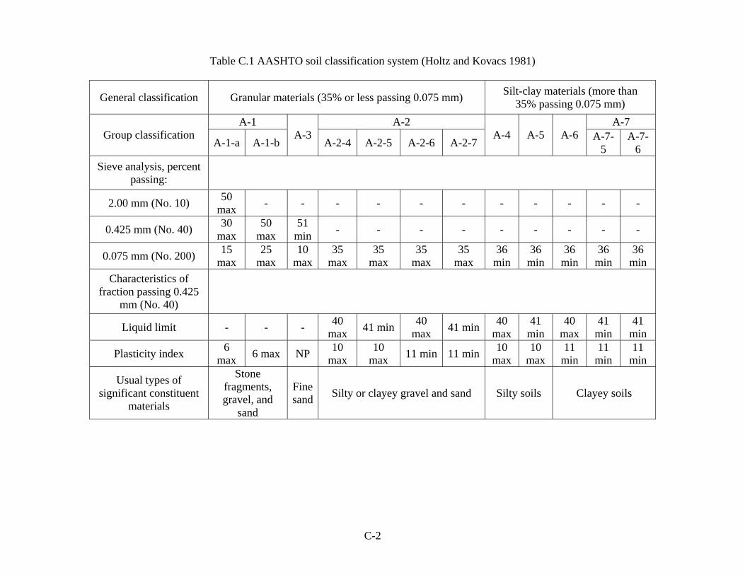
Table C.1 AASHTO soil classification system (Holtz and Kovacs 1981)
General classification Granular materials (35% or less passing 0.075 mm) Silt-clay materials (more than 35% passing 0.075 mm)
A-1 A-2 A-7 Group classification
A-1-a A-1-b A-3
A-2-4 A-2-5 A-2-6 A-2-7 A-4 A-5 A-6 A-7-
5 A-7-
6 Sieve analysis, percent
passing:
2.00 mm (No. 10) 50 max - - - - - - - - - - -
0.425 mm (No. 40) 30 max
50 max
51 min - - - - - - - - -
0.075 mm (No. 200) 15 max
25 max
10 max
35 max
35 max
35 max
35 max
36 min
36 min
36 min
36 min
36 min
Characteristics of fraction passing 0.425
mm (No. 40)
Liquid limit - - - 40 max 41 min 40
max 41 min 40 max
41 min
40 max
41 min
41 min
Plasticity index 6 max 6 max NP 10
max 10
max 11 min 11 min 10 max
10 max
11 min
11 min
11 min
Usual types of significant constituent
materials
Stone fragments, gravel, and
sand
Fine sand Silty or clayey gravel and sand Silty soils Clayey soils
C-3
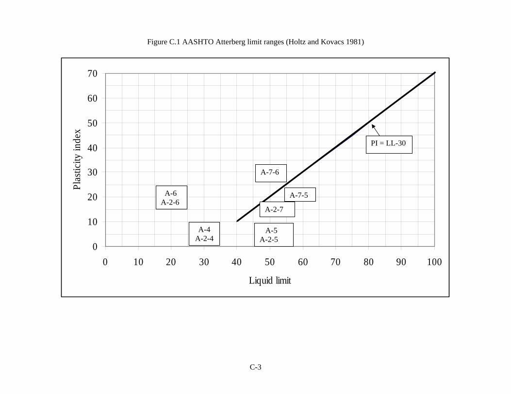
Figure C.1 AASHTO Atterberg limit ranges (Holtz and Kovacs 1981)
0
10
20
30
40
50
60
70
0 10 20 30 40 50 60 70 80 90 100
Liquid limit
Plas
ticity
inde
x
A-6 A-2-6
A-4 A-2-4
A-7-6
PI = LL-30
A-7-5
A-2-7
A-5 A-2-5
C-4
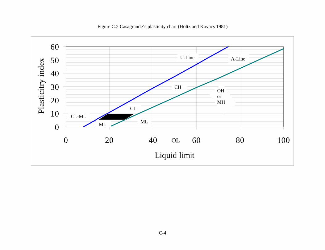
Figure C.2 Casagrande’s plasticity chart (Holtz and Kovacs 1981)
0102030405060
0 20 40 60 80 100
Liquid limit
Plas
ticitr
y in
dex
ML ML
CL
OL
OH or MH
CH
CL-ML
U-Line A-Line
C-5
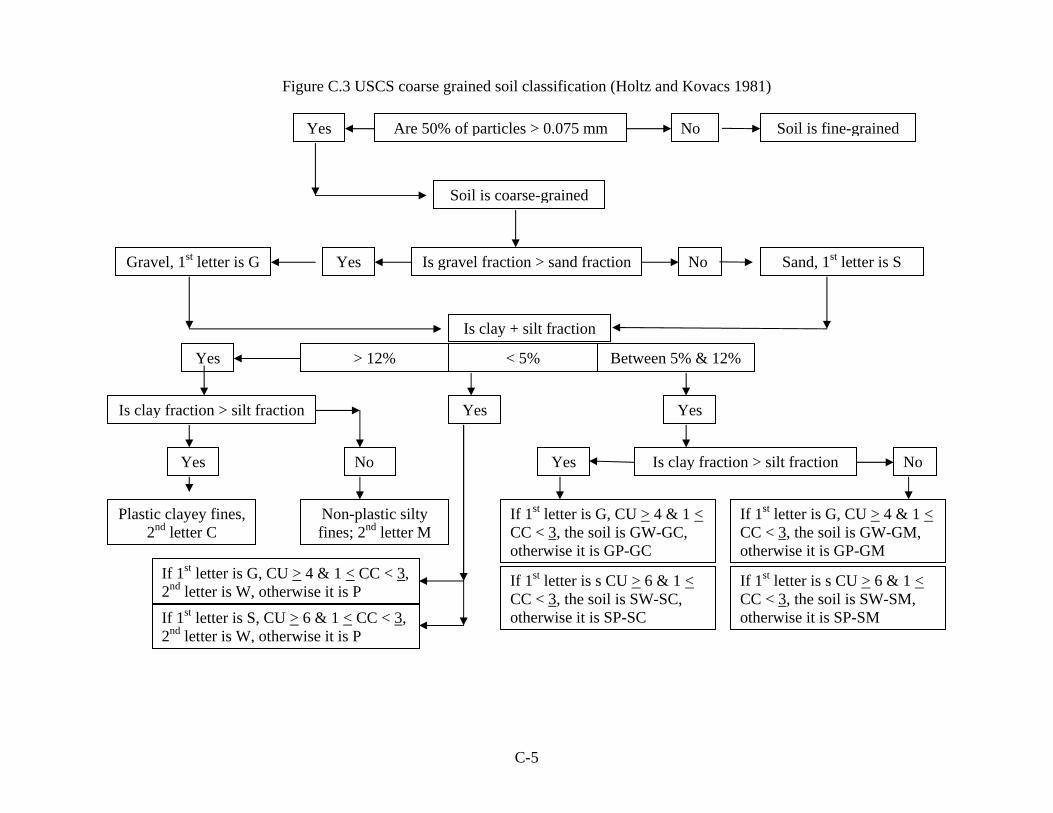
Figure C.3 USCS coarse grained soil classification (Holtz and Kovacs 1981)
Are 50% of particles > 0.075 mm
Soil is coarse-grained
Soil is fine-grained
Is gravel fraction > sand fraction Gravel, 1st letter is G Sand, 1st letter is S
Is clay + silt fraction
< 5%> 12% Between 5% & 12%
Is clay fraction > silt fraction
Is clay fraction > silt fraction
Non-plastic silty fines; 2nd letter M
Plastic clayey fines, 2nd letter C
NoYes
NoYes
Yes
Yes
Yes No
Yes
If 1st letter is G, CU > 4 & 1 < CC < 3, 2nd letter is W, otherwise it is PIf 1st letter is S, CU > 6 & 1 < CC < 3, 2nd letter is W, otherwise it is P
Yes No
If 1st letter is G, CU > 4 & 1 < CC < 3, the soil is GW-GC, otherwise it is GP-GC
If 1st letter is s CU > 6 & 1 < CC < 3, the soil is SW-SC, otherwise it is SP-SC
If 1st letter is G, CU > 4 & 1 < CC < 3, the soil is GW-GM, otherwise it is GP-GM
If 1st letter is s CU > 6 & 1 < CC < 3, the soil is SW-SM, otherwise it is SP-SM
C-6
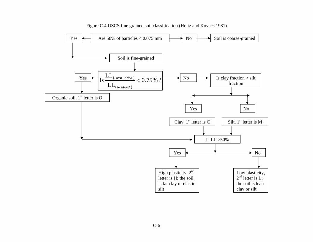
Figure C.4 USCS fine grained soil classification (Holtz and Kovacs 1981)
Are 50% of particles < 0.075 mm
Soil is fine-grained
Soil is coarse-grained
Organic soil, 1st letter is O
Is clay fraction > silt fraction
Is LL >50%
Clay, 1st letter is C
No Yes
No Yes
Yes
Yes
No
High plasticity, 2nd letter is H; the soil is fat clay or elastic silt
Low plasticity, 2nd letter is L; the soil is lean clay or silt
Silt, 1st letter is M
No
( )
( )?%75.0
LLLL
Is <−
Notdried
driedOven
C-7
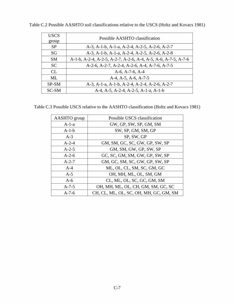
Table C.2 Possible AASHTO soil classifications relative to the USCS (Holtz and Kovacs 1981)
USCS group Possible AASHTO classification
SP A-3, A-1-b, A-1-a, A-2-4, A-2-5, A-2-6, A-2-7 SG A-3, A-1-b, A-1-a, A-2-4, A-2-5, A-2-6, A-2-8 SM A-1-b, A-2-4, A-2-5, A-2-7, A-2-6, A-4, A-5, A-6, A-7-5, A-7-6 SC A-2-6, A-2-7, A-2-4, A-2-6, A-4, A-7-6, A-7-5 CL A-6, A-7-6, A-4 ML A-4, A-5, A-6, A-7-5
SP-SM A-3, A-1-a, A-1-b, A-2-4, A-2-4, A-2-6, A-2-7 SC-SM A-4, A-5, A-2-4, A-2-5, A-1-a, A-1-b
Table C.3 Possible USCS relative to the AASHTO classification (Holtz and Kovacs 1981)
AASHTO group Possible USCS classification A-1-a GW, GP, SW, SP, GM, SM A-1-b SW, SP, GM, SM, GP A-3 SP, SW, GP
A-2-4 GM, SM, GC, SC, GW, GP, SW, SP A-2-5 GM, SM, GW, GP, SW, SP A-2-6 GC, SC, GM, SM, GW, GP, SW, SP A-2-7 GM, GC, SM, SC, GW, GP, SW, SP A-4 ML, OL, CL, SM, SC, GM, GC A-5 OH, MH, ML, OL, SM, GM A-6 CL, ML, OL, SC, GC, GM, SM
A-7-5 OH, MH, ML, OL, CH, GM, SM, GC, SC A-7-6 CH, CL, ML, OL, SC, OH, MH, GC, GM, SM

D-1
APPENDIX D
LABORATORY RESULTS
D-2
Figure D.1 Clusters of State of Michigan
D-3
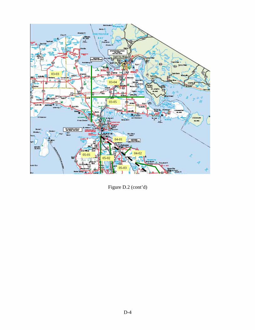
Figure D.2 Cluster and area boundaries in the State of Michigan
01-01
02-02
02-01 02-03
02-04
02-05
03-03
03-02
03-01
D-4
Figure D.2 (cont’d)
03-03
03-04
03-05
04-01
05-01 05-02
05-03
04-02
D-5
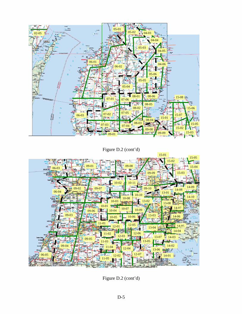
Figure D.2 (cont’d)
Figure D.2 (cont’d)
14-01
14-10
14-09 14-08
14-07
14-06
14-0514-04
14-03
14-02
10-01
09-02
09-01
09-07
09-06 09-03
09-04
09-05
13-0109-10
09-09
09-08
13-07
13-03
13-02
13-05
13-04
13-06
10-02
10-03
10-05 10-06
10-07
10-08
10-09
10-10
10-11
06-05
06-04
06-03 15-04
15-05 15-01
15-02
15-03
11-01
11-02
11-05
11-03
11-04 12-04
12-07
12-06
12-05
12-02
12-03
13-08
10-04
12-01
15-01
15-06
15-02 15-03
15-05
15-07
15-08 08-01
08-02
08-03
08-05
08-04
08-06 07-01
07-05
07-06
07-02
07-04 07-03
05-02
05-03
05-06
05-05
05-04
06-01 06-02
04-04
04-03
04-06
04-05
09-01 09-08
09-09
06-03
02-05 05-01
D-6
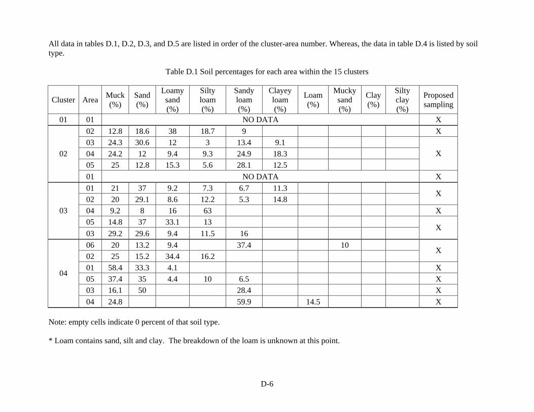
All data in tables D.1, D.2, D.3, and D.5 are listed in order of the cluster-area number. Whereas, the data in table D.4 is listed by soil type.
Table D.1 Soil percentages for each area within the 15 clusters
Cluster Area Muck (%)
Sand (%)
Loamy sand (%)
Silty loam (%)
Sandy loam (%)
Clayey loam (%)
Loam (%)
Mucky sand (%)
Clay (%)
Silty clay (%)
Proposed sampling
01 01 NO DATA X 02 12.8 18.6 38 18.7 9 X 03 24.3 30.6 12 3 13.4 9.1 04 24.2 12 9.4 9.3 24.9 18.3 05 25 12.8 15.3 5.6 28.1 12.5
X 02
01 NO DATA X 01 21 37 9.2 7.3 6.7 11.3 02 20 29.1 8.6 12.2 5.3 14.8
X
04 9.2 8 16 63 X 05 14.8 37 33.1 13
03
03 29.2 29.6 9.4 11.5 16 X
06 20 13.2 9.4 37.4 10 02 25 15.2 34.4 16.2
X
01 58.4 33.3 4.1 X 05 37.4 35 4.4 10 6.5 X 03 16.1 50 28.4 X
04
04 24.8 59.9 14.5 X
Note: empty cells indicate 0 percent of that soil type. * Loam contains sand, silt and clay. The breakdown of the loam is unknown at this point.

D-7
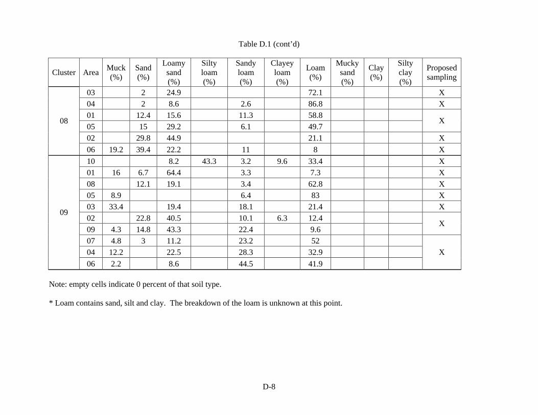
Table D.1 (cont’d)
Cluster Area Muck (%)
Sand (%)
Loamy sand (%)
Silty loam (%)
Sandy loam (%)
Clayey loam (%)
Loam (%)
Mucky sand (%)
Clay (%)
Silty clay (%)
Proposed sampling
01 22 5 72.4 X 02 13.1 41.5 39.3 03 14.3 74.7 7.8 2 04 26.3 51.4 17.4
X
05 97.9 1.7 X
05
06 4.4 14.4 25.2 13 39.2 X 01 3.3 53.5 30.4 9.3 X 02 8.1 71.8 7.5 8.2 X 03 8.1 75.6 5.9 4.7 X 04 25.7 39.5 8 26
06
05 23.6 41.6 12.2 17.1 X
04 14.9 6.8 11.4 65.3 X 02 63.2 7 25.1 X 05 2 18.4 18.6 7.9 48 X 03 6.2 53.9 26.3 12.7 X 01 15.1 32.1 28.6 10 10.1
07
06 13 34.3 36.6 7.5 7.1 X
Note: empty cells indicate 0 percent of that soil type. * Loam contains sand, silt and clay. The breakdown of the loam is unknown at this point.
D-8
Table D.1 (cont’d)
Cluster Area Muck (%)
Sand (%)
Loamy sand (%)
Silty loam (%)
Sandy loam (%)
Clayey loam (%)
Loam (%)
Mucky sand (%)
Clay (%)
Silty clay (%)
Proposed sampling
03 2 24.9 72.1 X 04 2 8.6 2.6 86.8 X 01 12.4 15.6 11.3 58.8 05 15 29.2 6.1 49.7
X
02 29.8 44.9 21.1 X
08
06 19.2 39.4 22.2 11 8 X 10 8.2 43.3 3.2 9.6 33.4 X 01 16 6.7 64.4 3.3 7.3 X 08 12.1 19.1 3.4 62.8 X 05 8.9 6.4 83 X 03 33.4 19.4 18.1 21.4 X 02 22.8 40.5 10.1 6.3 12.4 09 4.3 14.8 43.3 22.4 9.6
X
07 4.8 3 11.2 23.2 52 04 12.2 22.5 28.3 32.9
09
06 2.2 8.6 44.5 41.9 X
Note: empty cells indicate 0 percent of that soil type. * Loam contains sand, silt and clay. The breakdown of the loam is unknown at this point.
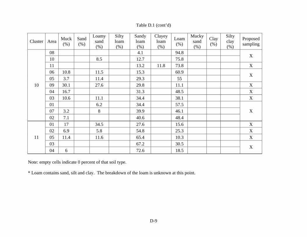
D-9
Table D.1 (cont’d)
Cluster Area Muck (%)
Sand (%)
Loamy sand (%)
Silty loam (%)
Sandy loam (%)
Clayey loam (%)
Loam (%)
Mucky sand (%)
Clay (%)
Silty clay (%)
Proposed sampling
08 4.1 94.8 10 8.5 12.7 75.8
X
11 13.2 11.8 73.8 X 06 10.8 11.5 15.3 60.9 05 3.7 11.4 29.3 55
X
09 30.1 27.6 29.8 11.1 X 04 16.7 31.3 48.5 X 03 10.6 11.1 34.4 38.1 X 01 6.2 34.4 57.5 07 3.2 8 39.9 46.1
10
02 7.1 40.6 48.4 X
01 17 34.5 27.6 15.6 X 02 6.9 5.8 54.8 25.3 X 05 11.4 11.6 65.4 10.3 X 03 67.2 30.5
11
04 6 72.6 18.5 X
Note: empty cells indicate 0 percent of that soil type. * Loam contains sand, silt and clay. The breakdown of the loam is unknown at this point.
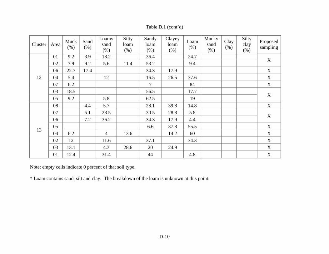
D-10
Table D.1 (cont’d)
Cluster Area Muck (%)
Sand (%)
Loamy sand (%)
Silty loam (%)
Sandy loam (%)
Clayey loam (%)
Loam (%)
Mucky sand (%)
Clay (%)
Silty clay (%)
Proposed sampling
01 9.2 3.9 18.2 36.4 24.7 02 7.9 9.2 5.6 11.4 53.2 9.4
X
06 22.7 17.4 34.3 17.9 X 04 5.4 12 16.5 26.5 37.6 X 07 6.2 7 84 X 03 18.5 56.5 17.7
12
05 9.2 5.8 62.5 19 X
08 4.4 5.7 28.1 39.8 14.8 X 07 5.1 28.5 30.5 28.8 5.8 06 7.2 36.2 34.3 17.9 4.4
X
05 6.6 37.8 55.5 X 04 6.2 4 13.6 14.2 60 X 02 12 11.6 37.1 34.3 X 03 13.1 4.3 28.6 20 24.9 X
13
01 12.4 31.4 44 4.8 X Note: empty cells indicate 0 percent of that soil type. * Loam contains sand, silt and clay. The breakdown of the loam is unknown at this point.
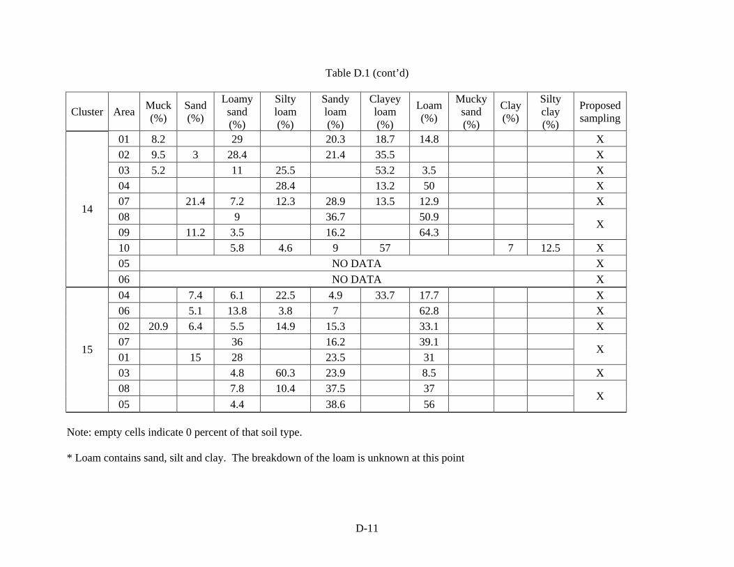
D-11
Table D.1 (cont’d)
Cluster Area Muck (%)
Sand (%)
Loamy sand (%)
Silty loam (%)
Sandy loam (%)
Clayey loam (%)
Loam (%)
Mucky sand (%)
Clay (%)
Silty clay (%)
Proposed sampling
01 8.2 29 20.3 18.7 14.8 X 02 9.5 3 28.4 21.4 35.5 X 03 5.2 11 25.5 53.2 3.5 X 04 28.4 13.2 50 X 07 21.4 7.2 12.3 28.9 13.5 12.9 X 08 9 36.7 50.9 09 11.2 3.5 16.2 64.3
X
10 5.8 4.6 9 57 7 12.5 X 05 NO DATA X
14
06 NO DATA X 04 7.4 6.1 22.5 4.9 33.7 17.7 X 06 5.1 13.8 3.8 7 62.8 X 02 20.9 6.4 5.5 14.9 15.3 33.1 X 07 36 16.2 39.1 01 15 28 23.5 31
X
03 4.8 60.3 23.9 8.5 X 08 7.8 10.4 37.5 37
15
05 4.4 38.6 56 X
Note: empty cells indicate 0 percent of that soil type. * Loam contains sand, silt and clay. The breakdown of the loam is unknown at this point
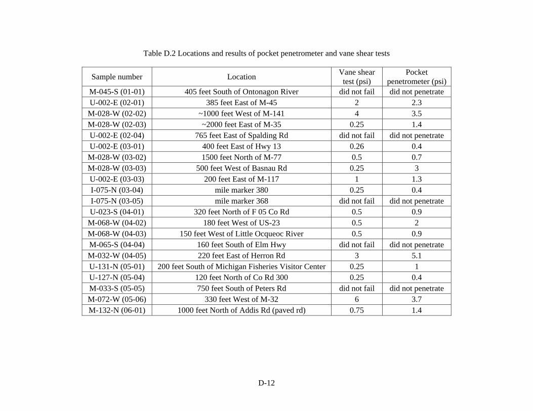
D-12
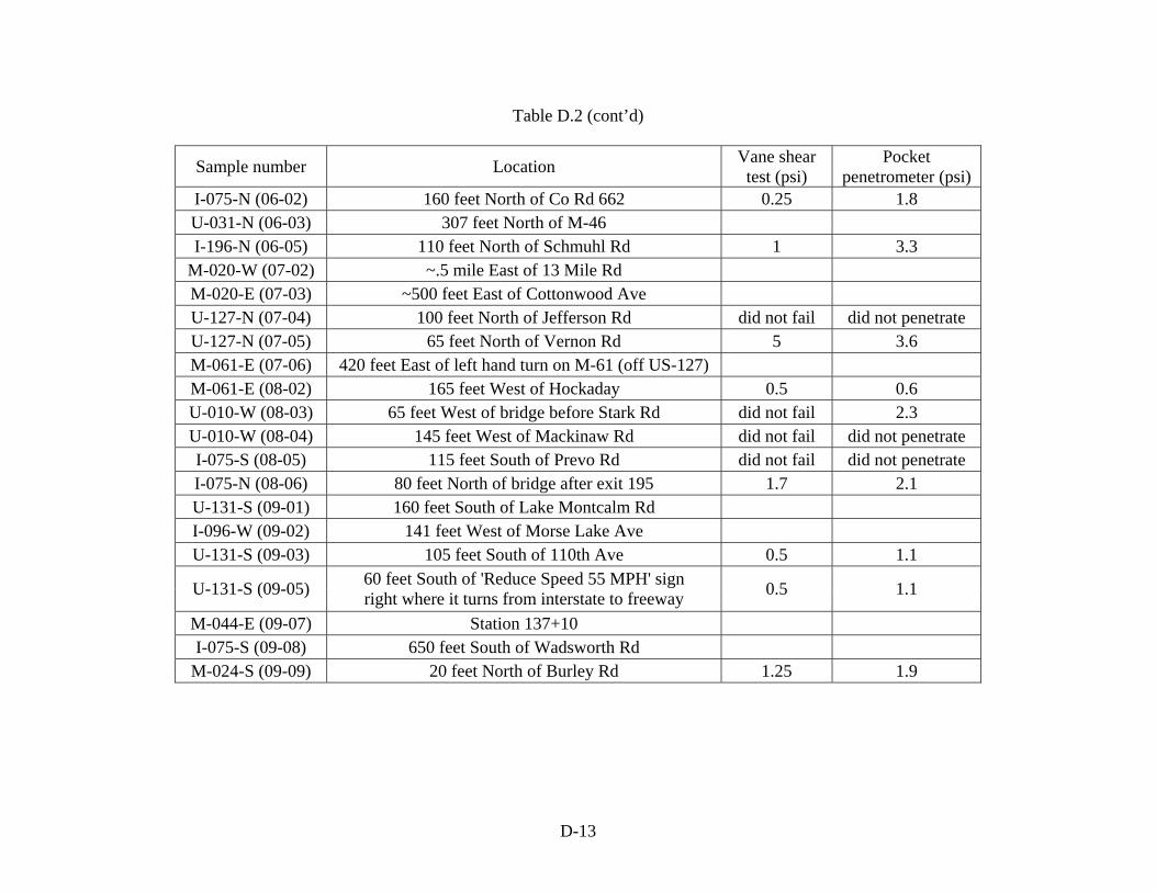
Table D.2 Locations and results of pocket penetrometer and vane shear tests
Sample number Location Vane shear test (psi)
Pocket penetrometer (psi)
M-045-S (01-01) 405 feet South of Ontonagon River did not fail did not penetrate U-002-E (02-01) 385 feet East of M-45 2 2.3 M-028-W (02-02) ~1000 feet West of M-141 4 3.5 M-028-W (02-03) ~2000 feet East of M-35 0.25 1.4 U-002-E (02-04) 765 feet East of Spalding Rd did not fail did not penetrate U-002-E (03-01) 400 feet East of Hwy 13 0.26 0.4 M-028-W (03-02) 1500 feet North of M-77 0.5 0.7 M-028-W (03-03) 500 feet West of Basnau Rd 0.25 3 U-002-E (03-03) 200 feet East of M-117 1 1.3 I-075-N (03-04) mile marker 380 0.25 0.4 I-075-N (03-05) mile marker 368 did not fail did not penetrate U-023-S (04-01) 320 feet North of F 05 Co Rd 0.5 0.9
M-068-W (04-02) 180 feet West of US-23 0.5 2 M-068-W (04-03) 150 feet West of Little Ocqueoc River 0.5 0.9 M-065-S (04-04) 160 feet South of Elm Hwy did not fail did not penetrate M-032-W (04-05) 220 feet East of Herron Rd 3 5.1 U-131-N (05-01) 200 feet South of Michigan Fisheries Visitor Center 0.25 1 U-127-N (05-04) 120 feet North of Co Rd 300 0.25 0.4 M-033-S (05-05) 750 feet South of Peters Rd did not fail did not penetrate M-072-W (05-06) 330 feet West of M-32 6 3.7 M-132-N (06-01) 1000 feet North of Addis Rd (paved rd) 0.75 1.4
D-13
Table D.2 (cont’d)
Sample number Location Vane shear test (psi)
Pocket penetrometer (psi)
I-075-N (06-02) 160 feet North of Co Rd 662 0.25 1.8 U-031-N (06-03) 307 feet North of M-46 I-196-N (06-05) 110 feet North of Schmuhl Rd 1 3.3
M-020-W (07-02) ~.5 mile East of 13 Mile Rd M-020-E (07-03) ~500 feet East of Cottonwood Ave U-127-N (07-04) 100 feet North of Jefferson Rd did not fail did not penetrate U-127-N (07-05) 65 feet North of Vernon Rd 5 3.6 M-061-E (07-06) 420 feet East of left hand turn on M-61 (off US-127) M-061-E (08-02) 165 feet West of Hockaday 0.5 0.6 U-010-W (08-03) 65 feet West of bridge before Stark Rd did not fail 2.3 U-010-W (08-04) 145 feet West of Mackinaw Rd did not fail did not penetrate I-075-S (08-05) 115 feet South of Prevo Rd did not fail did not penetrate I-075-N (08-06) 80 feet North of bridge after exit 195 1.7 2.1 U-131-S (09-01) 160 feet South of Lake Montcalm Rd I-096-W (09-02) 141 feet West of Morse Lake Ave U-131-S (09-03) 105 feet South of 110th Ave 0.5 1.1
U-131-S (09-05) 60 feet South of 'Reduce Speed 55 MPH' sign right where it turns from interstate to freeway 0.5 1.1
M-044-E (09-07) Station 137+10 I-075-S (09-08) 650 feet South of Wadsworth Rd
M-024-S (09-09) 20 feet North of Burley Rd 1.25 1.9

D-14
Table D.2 (cont’d)
Sample number Location Vane shear test (psi)
Pocket penetrometer (psi)
I-069-E (09-10) 172 feet East of Grand River Rd 0.5 1 I-069-N (10-01) 75 feet North of Base Line Hwy 3 4 I-096-W (10-03) 210 feet West of bridge before exit 97 1 1.3 I-069-N (10-04) 150 feet North of Island Hwy 1.75 4 I-069-N (10-05) 100 feet North of Five Points Hwy 2.5 3.2 I-096-W (10-09) 140 feet West of Dietz Rd 2.7 3.1 I-069-E (10-10) 120 feet East of Britton Rd did not fail did not penetrate
M-021-E (10-11) 800 feet East of Shepards Rd 3 2.6 I-069-N (11-01) 160 feet North of mile marker 42 I-094-W (11-02) 132 feet West of exit 110 on ramp 1.5 2.5
M-060-W (11-03) 135 feet West of Southbound I-69 overpass 3 5.5 I-069-S (11-05) 95 feet South of Bridge after exit 10 I-094-W (12-01) 95 feet West of 29 Mile Rd 1 2.6 I-094-W (12-03) 36 feet West of bridge after exit 135 1 1.5 U-012-E (12-04) 100 feet East of Emarld Rd did not fail 6 I-094-W (12-06) 53 feet West of Mt Hope Rd 3 3.5 U-012-E (12-07) 120 feet West of Person Hwy 0.5 0.9 M-024-S (13-01) 250 feet North of Best Rd 3.5 5 M-059-W (13-02) Station 131+29 M-014-W (13-03) 255 feet West of Napler Rd did not fail 4.5
D-15
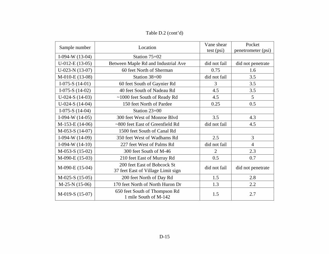
Table D.2 (cont’d)
Sample number Location Vane shear test (psi)
Pocket penetrometer (psi)
I-094-W (13-04) Station 75+02 U-012-E (13-05) Between Maple Rd and Industrial Ave did not fail did not penetrate U-023-N (13-07) 60 feet North of Sherman 0.75 1.6 M-010-E (13-08) Station 38+00 did not fail 3.5 I-075-S (14-01) 60 feet South of Gaynier Rd 3 3.5 I-075-S (14-02) 40 feet South of Nadeau Rd 4.5 3.5 U-024-S (14-03) ~1000 feet South of Ready Rd 4.5 5 U-024-S (14-04) 150 feet North of Pardee 0.25 0.5 I-075-S (14-04) Station 23+00 I-094-W (14-05) 300 feet West of Monroe Blvd 3.5 4.3 M-153-E (14-06) ~800 feet East of Greenfield Rd did not fail 4.5 M-053-S (14-07) 1500 feet South of Canal Rd I-094-W (14-09) 350 feet West of Wadhams Rd 2.5 3 I-094-W (14-10) 227 feet West of Palms Rd did not fail 4 M-053-S (15-02) 300 feet South of M-46 2 2.3 M-090-E (15-03) 210 feet East of Murray Rd 0.5 0.7
M-090-E (15-04) 200 feet East of Bobcock St 37 feet East of Village Limit sign did not fail did not penetrate
M-025-S (15-05) 200 feet North of Day Rd 1.5 2.8 M-25-N (15-06) 170 feet North of North Huron Dr 1.3 2.2
M-019-S (15-07) 650 feet South of Thompson Rd 1 mile South of M-142 1.5 2.7
D-16
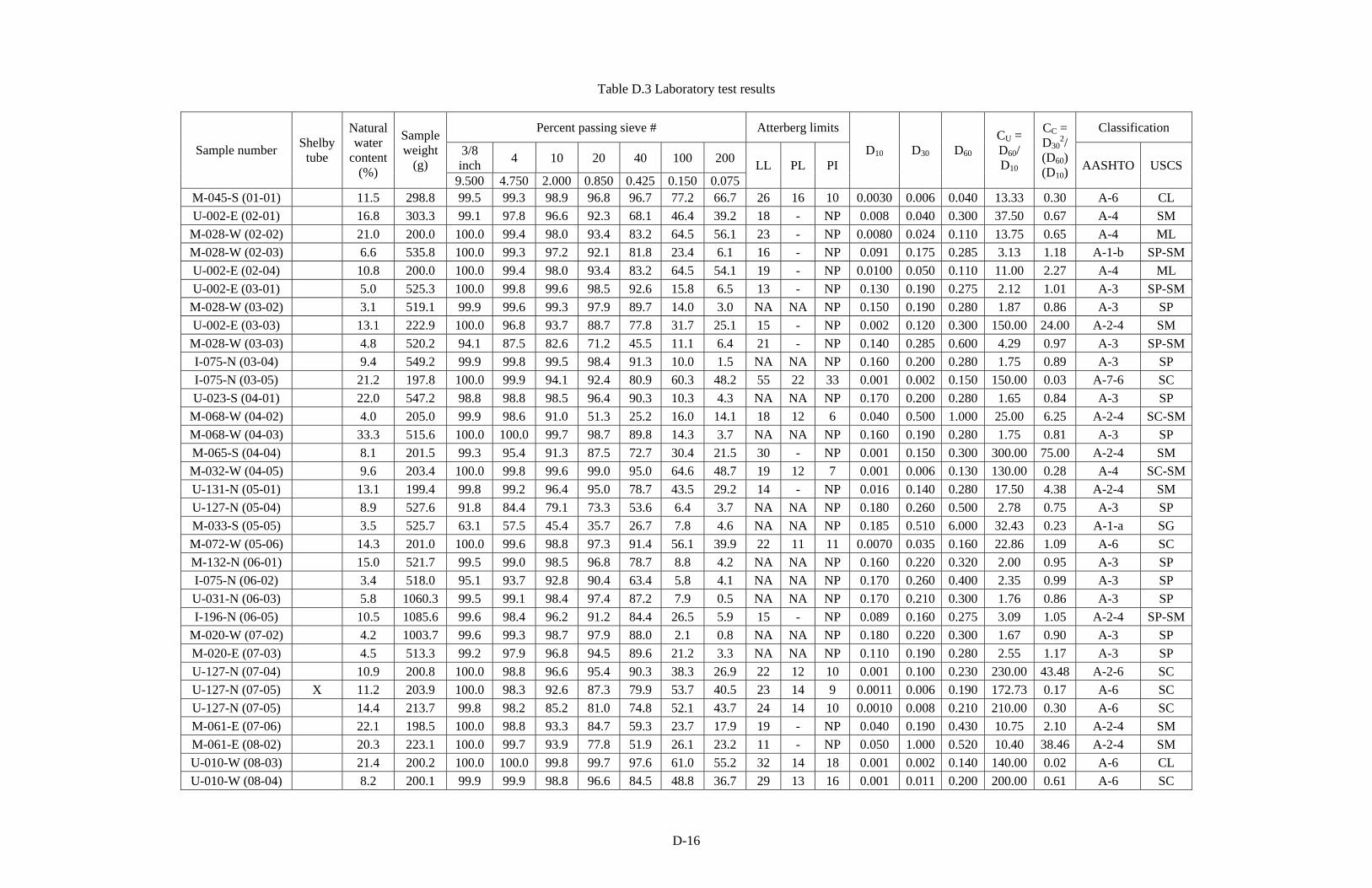
Table D.3 Laboratory test results
Percent passing sieve # Atterberg limits Classification
3/8 inch 4 10 20 40 100 200 Sample number Shelby
tube
Natural water
content (%)
Sample weight
(g) 9.500 4.750 2.000 0.850 0.425 0.150 0.075
LL PL PI D10 D30 D60
CU = D60/ D10
CC = D30
2/ (D60)(D10)
AASHTO USCS
M-045-S (01-01) 11.5 298.8 99.5 99.3 98.9 96.8 96.7 77.2 66.7 26 16 10 0.0030 0.006 0.040 13.33 0.30 A-6 CL U-002-E (02-01) 16.8 303.3 99.1 97.8 96.6 92.3 68.1 46.4 39.2 18 - NP 0.008 0.040 0.300 37.50 0.67 A-4 SM
M-028-W (02-02) 21.0 200.0 100.0 99.4 98.0 93.4 83.2 64.5 56.1 23 - NP 0.0080 0.024 0.110 13.75 0.65 A-4 ML M-028-W (02-03) 6.6 535.8 100.0 99.3 97.2 92.1 81.8 23.4 6.1 16 - NP 0.091 0.175 0.285 3.13 1.18 A-1-b SP-SM U-002-E (02-04) 10.8 200.0 100.0 99.4 98.0 93.4 83.2 64.5 54.1 19 - NP 0.0100 0.050 0.110 11.00 2.27 A-4 ML U-002-E (03-01) 5.0 525.3 100.0 99.8 99.6 98.5 92.6 15.8 6.5 13 - NP 0.130 0.190 0.275 2.12 1.01 A-3 SP-SM
M-028-W (03-02) 3.1 519.1 99.9 99.6 99.3 97.9 89.7 14.0 3.0 NA NA NP 0.150 0.190 0.280 1.87 0.86 A-3 SP U-002-E (03-03) 13.1 222.9 100.0 96.8 93.7 88.7 77.8 31.7 25.1 15 - NP 0.002 0.120 0.300 150.00 24.00 A-2-4 SM
M-028-W (03-03) 4.8 520.2 94.1 87.5 82.6 71.2 45.5 11.1 6.4 21 - NP 0.140 0.285 0.600 4.29 0.97 A-3 SP-SM I-075-N (03-04) 9.4 549.2 99.9 99.8 99.5 98.4 91.3 10.0 1.5 NA NA NP 0.160 0.200 0.280 1.75 0.89 A-3 SP I-075-N (03-05) 21.2 197.8 100.0 99.9 94.1 92.4 80.9 60.3 48.2 55 22 33 0.001 0.002 0.150 150.00 0.03 A-7-6 SC U-023-S (04-01) 22.0 547.2 98.8 98.8 98.5 96.4 90.3 10.3 4.3 NA NA NP 0.170 0.200 0.280 1.65 0.84 A-3 SP
M-068-W (04-02) 4.0 205.0 99.9 98.6 91.0 51.3 25.2 16.0 14.1 18 12 6 0.040 0.500 1.000 25.00 6.25 A-2-4 SC-SMM-068-W (04-03) 33.3 515.6 100.0 100.0 99.7 98.7 89.8 14.3 3.7 NA NA NP 0.160 0.190 0.280 1.75 0.81 A-3 SP M-065-S (04-04) 8.1 201.5 99.3 95.4 91.3 87.5 72.7 30.4 21.5 30 - NP 0.001 0.150 0.300 300.00 75.00 A-2-4 SM M-032-W (04-05) 9.6 203.4 100.0 99.8 99.6 99.0 95.0 64.6 48.7 19 12 7 0.001 0.006 0.130 130.00 0.28 A-4 SC-SMU-131-N (05-01) 13.1 199.4 99.8 99.2 96.4 95.0 78.7 43.5 29.2 14 - NP 0.016 0.140 0.280 17.50 4.38 A-2-4 SM U-127-N (05-04) 8.9 527.6 91.8 84.4 79.1 73.3 53.6 6.4 3.7 NA NA NP 0.180 0.260 0.500 2.78 0.75 A-3 SP M-033-S (05-05) 3.5 525.7 63.1 57.5 45.4 35.7 26.7 7.8 4.6 NA NA NP 0.185 0.510 6.000 32.43 0.23 A-1-a SG M-072-W (05-06) 14.3 201.0 100.0 99.6 98.8 97.3 91.4 56.1 39.9 22 11 11 0.0070 0.035 0.160 22.86 1.09 A-6 SC M-132-N (06-01) 15.0 521.7 99.5 99.0 98.5 96.8 78.7 8.8 4.2 NA NA NP 0.160 0.220 0.320 2.00 0.95 A-3 SP I-075-N (06-02) 3.4 518.0 95.1 93.7 92.8 90.4 63.4 5.8 4.1 NA NA NP 0.170 0.260 0.400 2.35 0.99 A-3 SP U-031-N (06-03) 5.8 1060.3 99.5 99.1 98.4 97.4 87.2 7.9 0.5 NA NA NP 0.170 0.210 0.300 1.76 0.86 A-3 SP I-196-N (06-05) 10.5 1085.6 99.6 98.4 96.2 91.2 84.4 26.5 5.9 15 - NP 0.089 0.160 0.275 3.09 1.05 A-2-4 SP-SM
M-020-W (07-02) 4.2 1003.7 99.6 99.3 98.7 97.9 88.0 2.1 0.8 NA NA NP 0.180 0.220 0.300 1.67 0.90 A-3 SP M-020-E (07-03) 4.5 513.3 99.2 97.9 96.8 94.5 89.6 21.2 3.3 NA NA NP 0.110 0.190 0.280 2.55 1.17 A-3 SP U-127-N (07-04) 10.9 200.8 100.0 98.8 96.6 95.4 90.3 38.3 26.9 22 12 10 0.001 0.100 0.230 230.00 43.48 A-2-6 SC U-127-N (07-05) X 11.2 203.9 100.0 98.3 92.6 87.3 79.9 53.7 40.5 23 14 9 0.0011 0.006 0.190 172.73 0.17 A-6 SC U-127-N (07-05) 14.4 213.7 99.8 98.2 85.2 81.0 74.8 52.1 43.7 24 14 10 0.0010 0.008 0.210 210.00 0.30 A-6 SC M-061-E (07-06) 22.1 198.5 100.0 98.8 93.3 84.7 59.3 23.7 17.9 19 - NP 0.040 0.190 0.430 10.75 2.10 A-2-4 SM M-061-E (08-02) 20.3 223.1 100.0 99.7 93.9 77.8 51.9 26.1 23.2 11 - NP 0.050 1.000 0.520 10.40 38.46 A-2-4 SM U-010-W (08-03) 21.4 200.2 100.0 100.0 99.8 99.7 97.6 61.0 55.2 32 14 18 0.001 0.002 0.140 140.00 0.02 A-6 CL U-010-W (08-04) 8.2 200.1 99.9 99.9 98.8 96.6 84.5 48.8 36.7 29 13 16 0.001 0.011 0.200 200.00 0.61 A-6 SC
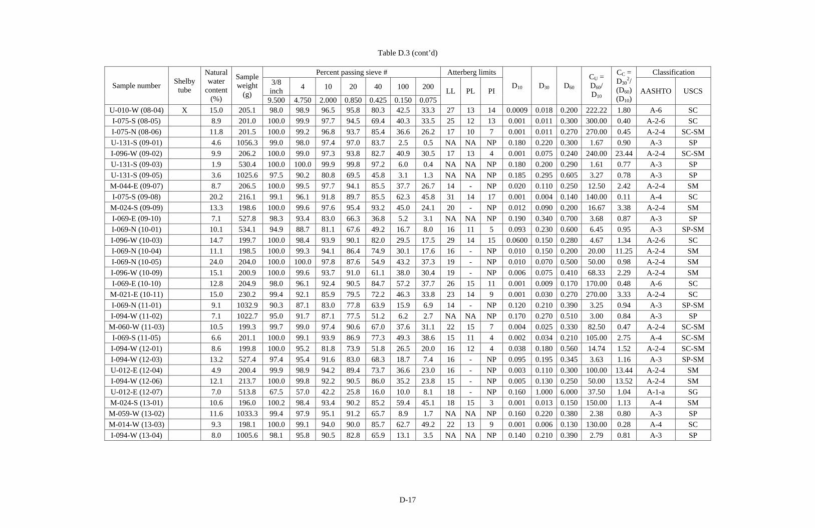
D-17
Table D.3 (cont’d)
Percent passing sieve # Atterberg limits Classification 3/8 inch 4 10 20 40 100 200 Sample number Shelby
tube
Natural water
content (%)
Sample weight
(g) 9.500 4.750 2.000 0.850 0.425 0.150 0.075
LL PL PI D10 D30 D60
CU = D60/ D10
CC = D30
2/ (D60)(D10)
AASHTO USCS
U-010-W (08-04) X 15.0 205.1 98.0 98.9 96.5 95.8 80.3 42.5 33.3 27 13 14 0.0009 0.018 0.200 222.22 1.80 A-6 SC I-075-S (08-05) 8.9 201.0 100.0 99.9 97.7 94.5 69.4 40.3 33.5 25 12 13 0.001 0.011 0.300 300.00 0.40 A-2-6 SC I-075-N (08-06) 11.8 201.5 100.0 99.2 96.8 93.7 85.4 36.6 26.2 17 10 7 0.001 0.011 0.270 270.00 0.45 A-2-4 SC-SM U-131-S (09-01) 4.6 1056.3 99.0 98.0 97.4 97.0 83.7 2.5 0.5 NA NA NP 0.180 0.220 0.300 1.67 0.90 A-3 SP I-096-W (09-02) 9.9 206.2 100.0 99.0 97.3 93.8 82.7 40.9 30.5 17 13 4 0.001 0.075 0.240 240.00 23.44 A-2-4 SC-SM U-131-S (09-03) 1.9 530.4 100.0 100.0 99.9 99.8 97.2 6.0 0.4 NA NA NP 0.180 0.200 0.290 1.61 0.77 A-3 SP U-131-S (09-05) 3.6 1025.6 97.5 90.2 80.8 69.5 45.8 3.1 1.3 NA NA NP 0.185 0.295 0.605 3.27 0.78 A-3 SP M-044-E (09-07) 8.7 206.5 100.0 99.5 97.7 94.1 85.5 37.7 26.7 14 - NP 0.020 0.110 0.250 12.50 2.42 A-2-4 SM I-075-S (09-08) 20.2 216.1 99.1 96.1 91.8 89.7 85.5 62.3 45.8 31 14 17 0.001 0.004 0.140 140.00 0.11 A-4 SC
M-024-S (09-09) 13.3 198.6 100.0 99.6 97.6 95.4 93.2 45.0 24.1 20 - NP 0.012 0.090 0.200 16.67 3.38 A-2-4 SM I-069-E (09-10) 7.1 527.8 98.3 93.4 83.0 66.3 36.8 5.2 3.1 NA NA NP 0.190 0.340 0.700 3.68 0.87 A-3 SP I-069-N (10-01) 10.1 534.1 94.9 88.7 81.1 67.6 49.2 16.7 8.0 16 11 5 0.093 0.230 0.600 6.45 0.95 A-3 SP-SM I-096-W (10-03) 14.7 199.7 100.0 98.4 93.9 90.1 82.0 29.5 17.5 29 14 15 0.0600 0.150 0.280 4.67 1.34 A-2-6 SC I-069-N (10-04) 11.1 198.5 100.0 99.3 94.1 86.4 74.9 30.1 17.6 16 - NP 0.010 0.150 0.200 20.00 11.25 A-2-4 SM I-069-N (10-05) 24.0 204.0 100.0 100.0 97.8 87.6 54.9 43.2 37.3 19 - NP 0.010 0.070 0.500 50.00 0.98 A-2-4 SM I-096-W (10-09) 15.1 200.9 100.0 99.6 93.7 91.0 61.1 38.0 30.4 19 - NP 0.006 0.075 0.410 68.33 2.29 A-2-4 SM I-069-E (10-10) 12.8 204.9 98.0 96.1 92.4 90.5 84.7 57.2 37.7 26 15 11 0.001 0.009 0.170 170.00 0.48 A-6 SC
M-021-E (10-11) 15.0 230.2 99.4 92.1 85.9 79.5 72.2 46.3 33.8 23 14 9 0.001 0.030 0.270 270.00 3.33 A-2-4 SC I-069-N (11-01) 9.1 1032.9 90.3 87.1 83.0 77.8 63.9 15.9 6.9 14 - NP 0.120 0.210 0.390 3.25 0.94 A-3 SP-SM I-094-W (11-02) 7.1 1022.7 95.0 91.7 87.1 77.5 51.2 6.2 2.7 NA NA NP 0.170 0.270 0.510 3.00 0.84 A-3 SP
M-060-W (11-03) 10.5 199.3 99.7 99.0 97.4 90.6 67.0 37.6 31.1 22 15 7 0.004 0.025 0.330 82.50 0.47 A-2-4 SC-SM I-069-S (11-05) 6.6 201.1 100.0 99.1 93.9 86.9 77.3 49.3 38.6 15 11 4 0.002 0.034 0.210 105.00 2.75 A-4 SC-SM I-094-W (12-01) 8.6 199.8 100.0 95.2 81.8 73.9 51.8 26.5 20.0 16 12 4 0.038 0.180 0.560 14.74 1.52 A-2-4 SC-SM I-094-W (12-03) 13.2 527.4 97.4 95.4 91.6 83.0 68.3 18.7 7.4 16 - NP 0.095 0.195 0.345 3.63 1.16 A-3 SP-SM U-012-E (12-04) 4.9 200.4 99.9 98.9 94.2 89.4 73.7 36.6 23.0 16 - NP 0.003 0.110 0.300 100.00 13.44 A-2-4 SM I-094-W (12-06) 12.1 213.7 100.0 99.8 92.2 90.5 86.0 35.2 23.8 15 - NP 0.005 0.130 0.250 50.00 13.52 A-2-4 SM U-012-E (12-07) 7.0 513.8 67.5 57.0 42.2 25.8 16.0 10.0 8.1 18 - NP 0.160 1.000 6.000 37.50 1.04 A-1-a SG M-024-S (13-01) 10.6 196.0 100.2 98.4 93.4 90.2 85.2 59.4 45.1 18 15 3 0.001 0.013 0.150 150.00 1.13 A-4 SM M-059-W (13-02) 11.6 1033.3 99.4 97.9 95.1 91.2 65.7 8.9 1.7 NA NA NP 0.160 0.220 0.380 2.38 0.80 A-3 SP M-014-W (13-03) 9.3 198.1 100.0 99.1 94.0 90.0 85.7 62.7 49.2 22 13 9 0.001 0.006 0.130 130.00 0.28 A-4 SC I-094-W (13-04) 8.0 1005.6 98.1 95.8 90.5 82.8 65.9 13.1 3.5 NA NA NP 0.140 0.210 0.390 2.79 0.81 A-3 SP
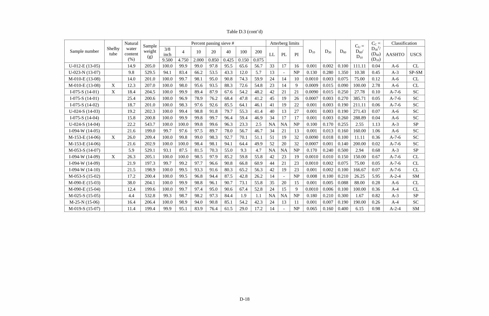
D-18
Table D.3 (cont’d)
Percent passing sieve # Atterberg limits Classification 3/8 inch 4 10 20 40 100 200 Sample number Shelby
tube
Natural water
content (%)
Sample weight
(g) 9.500 4.750 2.000 0.850 0.425 0.150 0.075
LL PL PI D10 D30 D60
CU = D60/ D10
CC = D30
2/ (D60)(D10)
AASHTO USCS
U-012-E (13-05) 14.9 205.0 100.0 99.9 99.0 97.8 95.5 65.6 56.7 33 17 16 0.001 0.002 0.100 111.11 0.04 A-6 CL U-023-N (13-07) 9.8 529.5 94.1 83.4 66.2 53.5 43.3 12.0 5.7 13 - NP 0.130 0.280 1.350 10.38 0.45 A-3 SP-SMM-010-E (13-08) 14.0 201.0 100.0 99.7 98.1 95.0 90.8 74.3 59.9 24 14 10 0.0010 0.003 0.075 75.00 0.12 A-6 CL M-010-E (13-08) X 12.3 207.0 100.0 98.0 95.6 93.5 88.3 72.6 54.8 23 14 9 0.0009 0.015 0.090 100.00 2.78 A-6 CL I-075-S (14-01) X 18.4 204.5 100.0 99.9 89.4 87.9 67.6 54.2 48.2 42 21 21 0.0090 0.015 0.250 27.78 0.10 A-7-6 SC I-075-S (14-01) 25.4 200.6 100.0 96.9 78.9 76.2 68.4 47.8 41.2 45 19 26 0.0007 0.003 0.270 385.71 0.05 A-7-6 SC I-075-S (14-02) 18.7 201.0 100.0 98.3 97.6 92.6 85.5 64.1 46.1 41 19 22 0.001 0.003 0.190 211.11 0.06 A-7-6 SC U-024-S (14-03) 19.2 202.3 100.0 99.4 98.8 91.8 79.7 55.3 41.4 40 13 27 0.001 0.003 0.190 271.43 0.07 A-6 SC I-075-S (14-04) 15.8 200.8 100.0 99.9 99.8 99.7 96.4 59.4 46.9 34 17 17 0.001 0.003 0.260 288.89 0.04 A-6 SC U-024-S (14-04) 22.2 543.7 100.0 100.0 99.8 99.6 96.3 23.3 2.5 NA NA NP 0.100 0.170 0.255 2.55 1.13 A-3 SP I-094-W (14-05) 21.6 199.0 99.7 97.6 97.5 89.7 78.0 56.7 46.7 34 21 13 0.001 0.013 0.160 160.00 1.06 A-6 SC M-153-E (14-06) X 26.0 209.4 100.0 99.8 99.0 98.3 92.7 70.1 51.1 51 19 32 0.0090 0.018 0.100 11.11 0.36 A-7-6 SC M-153-E (14-06) 21.6 202.9 100.0 100.0 98.4 98.1 94.1 64.4 49.9 52 20 32 0.0007 0.001 0.140 200.00 0.02 A-7-6 SC M-053-S (14-07) 5.9 529.1 93.1 87.5 81.5 70.3 55.0 9.3 4.7 NA NA NP 0.170 0.240 0.500 2.94 0.68 A-3 SP I-094-W (14-09) X 26.3 205.1 100.0 100.0 98.5 97.9 85.2 59.8 55.8 42 23 19 0.0010 0.010 0.150 150.00 0.67 A-7-6 CL I-094-W (14-09) 21.9 197.3 99.7 99.2 97.7 96.6 90.8 66.8 60.9 44 21 23 0.0010 0.002 0.075 75.00 0.05 A-7-6 CL I-094-W (14-10) 21.5 198.9 100.0 99.5 93.3 91.6 80.3 65.2 56.3 42 19 23 0.001 0.002 0.100 166.67 0.07 A-7-6 CL M-053-S (15-02) 17.2 200.4 100.0 99.5 96.8 94.4 87.5 42.8 26.2 14 - NP 0.008 0.100 0.210 26.25 5.95 A-2-4 SM M-090-E (15-03) 38.0 204.1 100.0 99.9 98.8 96.1 90.7 73.1 55.8 35 20 15 0.001 0.005 0.088 88.00 0.28 A-6 CL M-090-E (15-04) 12.4 199.6 100.0 99.7 97.4 95.0 90.6 67.4 52.8 24 15 9 0.0010 0.006 0.100 100.00 0.36 A-4 CL M-025-S (15-05) 4.4 532.8 99.3 98.7 98.2 97.3 84.4 1.9 1.1 NA NA NP 0.180 0.210 0.300 1.67 0.82 A-3 SP M-25-N (15-06) 16.4 206.4 100.0 98.9 94.0 90.8 85.1 54.2 42.3 24 13 11 0.001 0.007 0.190 190.00 0.26 A-4 SC M-019-S (15-07) 11.4 199.4 99.9 95.1 83.9 76.4 61.5 29.0 17.2 14 - NP 0.065 0.160 0.400 6.15 0.98 A-2-4 SM
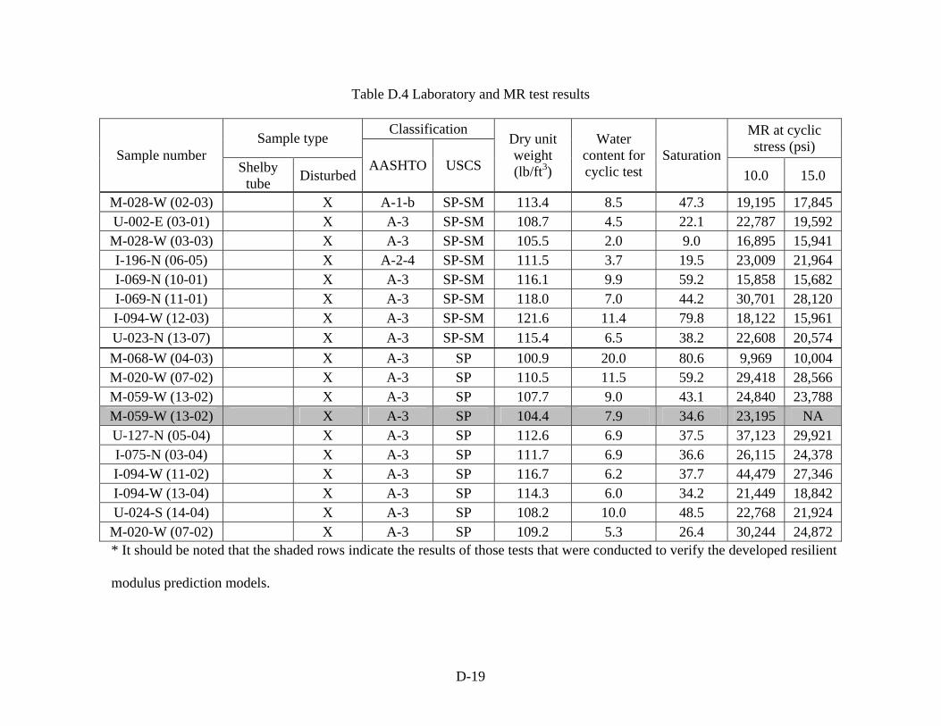
D-19
Table D.4 Laboratory and MR test results
Classification Sample type MR at cyclic stress (psi) Sample number
Shelby tube Disturbed
AASHTO USCS
Dry unit weight (lb/ft3)
Water content for cyclic test
Saturation10.0 15.0
M-028-W (02-03) X A-1-b SP-SM 113.4 8.5 47.3 19,195 17,845 U-002-E (03-01) X A-3 SP-SM 108.7 4.5 22.1 22,787 19,592 M-028-W (03-03) X A-3 SP-SM 105.5 2.0 9.0 16,895 15,941 I-196-N (06-05) X A-2-4 SP-SM 111.5 3.7 19.5 23,009 21,964 I-069-N (10-01) X A-3 SP-SM 116.1 9.9 59.2 15,858 15,682 I-069-N (11-01) X A-3 SP-SM 118.0 7.0 44.2 30,701 28,120 I-094-W (12-03) X A-3 SP-SM 121.6 11.4 79.8 18,122 15,961 U-023-N (13-07) X A-3 SP-SM 115.4 6.5 38.2 22,608 20,574 M-068-W (04-03) X A-3 SP 100.9 20.0 80.6 9,969 10,004 M-020-W (07-02) X A-3 SP 110.5 11.5 59.2 29,418 28,566 M-059-W (13-02) X A-3 SP 107.7 9.0 43.1 24,840 23,788 M-059-W (13-02) X A-3 SP 104.4 7.9 34.6 23,195 NA U-127-N (05-04) X A-3 SP 112.6 6.9 37.5 37,123 29,921 I-075-N (03-04) X A-3 SP 111.7 6.9 36.6 26,115 24,378 I-094-W (11-02) X A-3 SP 116.7 6.2 37.7 44,479 27,346 I-094-W (13-04) X A-3 SP 114.3 6.0 34.2 21,449 18,842 U-024-S (14-04) X A-3 SP 108.2 10.0 48.5 22,768 21,924
M-020-W (07-02) X A-3 SP 109.2 5.3 26.4 30,244 24,872 * It should be noted that the shaded rows indicate the results of those tests that were conducted to verify the developed resilient
modulus prediction models.

D-20
Table D.4 (cont’d)
Classification Sample type MR at cyclic stress (psi) Sample number
Shelby tube Disturbed
AASHTO USCS
Dry unit weight (lb/ft3)
Water content for cyclic test
Saturation10.0 15.0
I-069-E (09-10) X A-3 SP 116.9 5.1 31.2 28,636 26,070 M-132-N (06-01) X A-3 SP 112.9 4.7 25.8 31,711 28,970 M-053-S (14-07) X A-3 SP 113.9 3.9 22.0 25,714 22,275 U-023-S (04-01) X A-3 SP 117.8 3.3 20.7 23,039 21,715 U-031-N (06-03) X A-3 SP 111.5 3.3 17.4 31,870 29,609 M-020-E (07-03) X A-3 SP 113.0 3.2 17.6 32,666 28,156 M-025-S (15-05) X A-3 SP 110.3 3.0 15.4 40,115 35,447 U-131-S (09-01) X A-3 SP 110.6 2.7 13.9 28,766 27,706 I-075-N (06-02) X A-3 SP 110.2 2.0 10.2 32,457 31,187 U-131-S (09-05) X A-3 SP 117.3 1.0 23.3 38,423 35,319
M-028-W (03-02) X A-3 SP 104.0 1.3 5.7 22,959 22,494 U-131-S (09-03) X A-3 SP 108.6 0.5 2.4 30,340 27,995
M-020-W (07-02) X A-3 SP 109.1 0.2 1.0 31,460 28,705 M-020-W (07-02) X A-3 SP 104.1 0.2 0.9 19,692 20,267 M-020-W (07-02) X A-3 SP 107.6 0.2 1.0 24,319 24,552 U-002-E (02-01) X A-4 SM 109.3 9.5 47.4 15,352 13,818 U-002-E (03-03) X A-2-4 SM 111.5 7.7 40.7 15,969 15,818 M-065-S (04-04) X A-2-4 SM 94.6 7.6 26.3 11,932 11,898 U-131-N (05-01) X A-2-4 SM 112.9 5.4 29.6 24,627 23,092 M-061-E (07-06) X A-2-4 SM 96.0 17.0 60.8 11,480 12,958 M-061-E (08-02) X A-2-4 SM 118.6 5.5 35.3 32,200 31,733 M-044-E (09-07) X A-2-4 SM 128.8 7.6 66.6 18,416 19,636
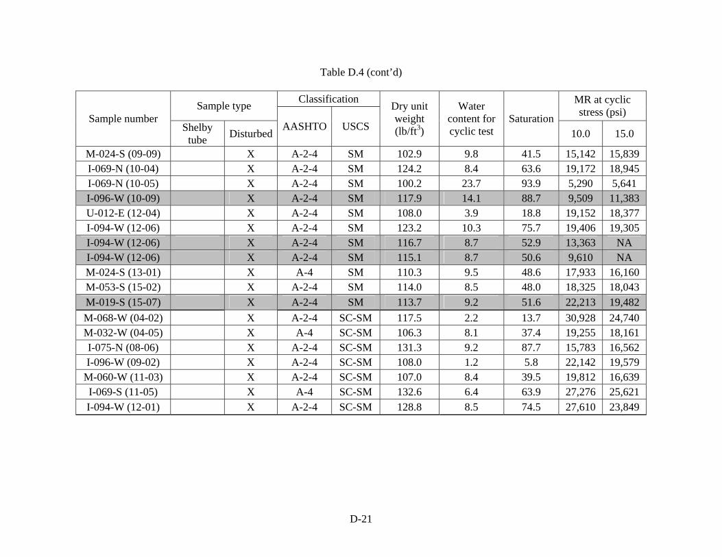
D-21
Table D.4 (cont’d)
Classification Sample type MR at cyclic stress (psi) Sample number
Shelby tube Disturbed
AASHTO USCS
Dry unit weight (lb/ft3)
Water content for cyclic test
Saturation10.0 15.0
M-024-S (09-09) X A-2-4 SM 102.9 9.8 41.5 15,142 15,839 I-069-N (10-04) X A-2-4 SM 124.2 8.4 63.6 19,172 18,945 I-069-N (10-05) X A-2-4 SM 100.2 23.7 93.9 5,290 5,641 I-096-W (10-09) X A-2-4 SM 117.9 14.1 88.7 9,509 11,383 U-012-E (12-04) X A-2-4 SM 108.0 3.9 18.8 19,152 18,377 I-094-W (12-06) X A-2-4 SM 123.2 10.3 75.7 19,406 19,305 I-094-W (12-06) X A-2-4 SM 116.7 8.7 52.9 13,363 NA I-094-W (12-06) X A-2-4 SM 115.1 8.7 50.6 9,610 NA M-024-S (13-01) X A-4 SM 110.3 9.5 48.6 17,933 16,160 M-053-S (15-02) X A-2-4 SM 114.0 8.5 48.0 18,325 18,043 M-019-S (15-07) X A-2-4 SM 113.7 9.2 51.6 22,213 19,482 M-068-W (04-02) X A-2-4 SC-SM 117.5 2.2 13.7 30,928 24,740 M-032-W (04-05) X A-4 SC-SM 106.3 8.1 37.4 19,255 18,161 I-075-N (08-06) X A-2-4 SC-SM 131.3 9.2 87.7 15,783 16,562 I-096-W (09-02) X A-2-4 SC-SM 108.0 1.2 5.8 22,142 19,579
M-060-W (11-03) X A-2-4 SC-SM 107.0 8.4 39.5 19,812 16,639 I-069-S (11-05) X A-4 SC-SM 132.6 6.4 63.9 27,276 25,621 I-094-W (12-01) X A-2-4 SC-SM 128.8 8.5 74.5 27,610 23,849
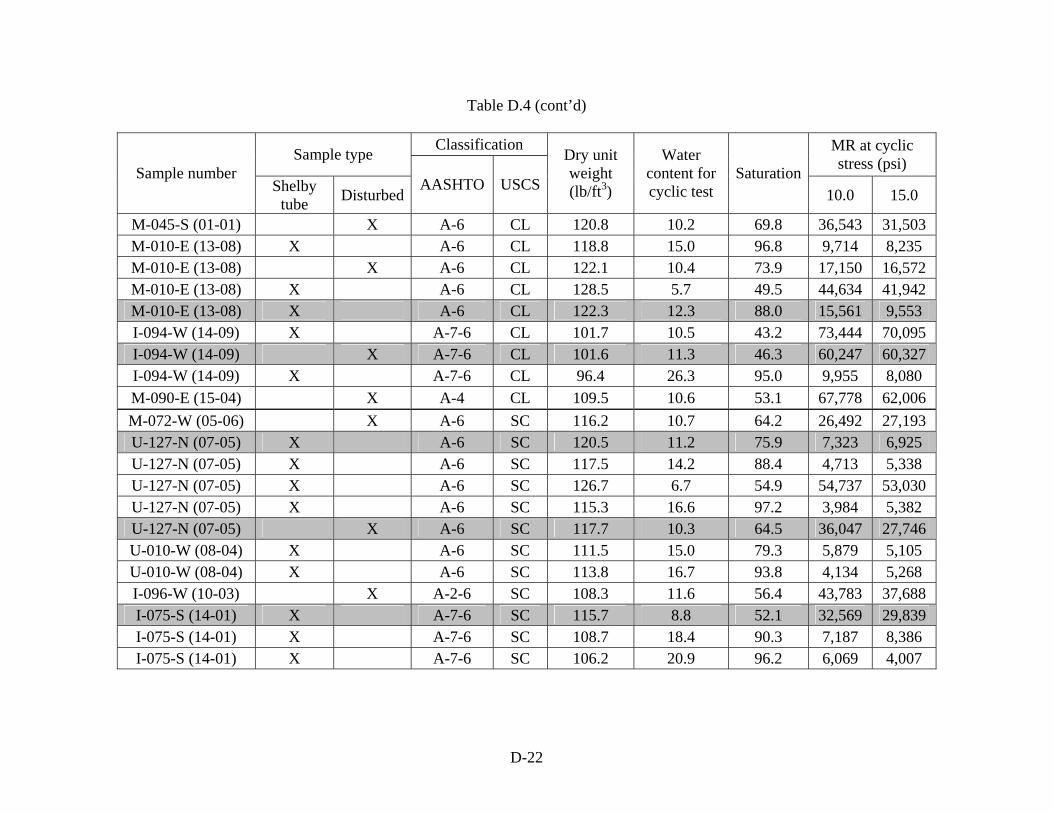
D-22
Table D.4 (cont’d)
Classification Sample type MR at cyclic stress (psi) Sample number
Shelby tube Disturbed
AASHTO USCS
Dry unit weight (lb/ft3)
Water content for cyclic test
Saturation10.0 15.0
M-045-S (01-01) X A-6 CL 120.8 10.2 69.8 36,543 31,503 M-010-E (13-08) X A-6 CL 118.8 15.0 96.8 9,714 8,235 M-010-E (13-08) X A-6 CL 122.1 10.4 73.9 17,150 16,572 M-010-E (13-08) X A-6 CL 128.5 5.7 49.5 44,634 41,942 M-010-E (13-08) X A-6 CL 122.3 12.3 88.0 15,561 9,553 I-094-W (14-09) X A-7-6 CL 101.7 10.5 43.2 73,444 70,095 I-094-W (14-09) X A-7-6 CL 101.6 11.3 46.3 60,247 60,327 I-094-W (14-09) X A-7-6 CL 96.4 26.3 95.0 9,955 8,080 M-090-E (15-04) X A-4 CL 109.5 10.6 53.1 67,778 62,006 M-072-W (05-06) X A-6 SC 116.2 10.7 64.2 26,492 27,193 U-127-N (07-05) X A-6 SC 120.5 11.2 75.9 7,323 6,925 U-127-N (07-05) X A-6 SC 117.5 14.2 88.4 4,713 5,338 U-127-N (07-05) X A-6 SC 126.7 6.7 54.9 54,737 53,030 U-127-N (07-05) X A-6 SC 115.3 16.6 97.2 3,984 5,382 U-127-N (07-05) X A-6 SC 117.7 10.3 64.5 36,047 27,746 U-010-W (08-04) X A-6 SC 111.5 15.0 79.3 5,879 5,105 U-010-W (08-04) X A-6 SC 113.8 16.7 93.8 4,134 5,268 I-096-W (10-03) X A-2-6 SC 108.3 11.6 56.4 43,783 37,688 I-075-S (14-01) X A-7-6 SC 115.7 8.8 52.1 32,569 29,839 I-075-S (14-01) X A-7-6 SC 108.7 18.4 90.3 7,187 8,386 I-075-S (14-01) X A-7-6 SC 106.2 20.9 96.2 6,069 4,007
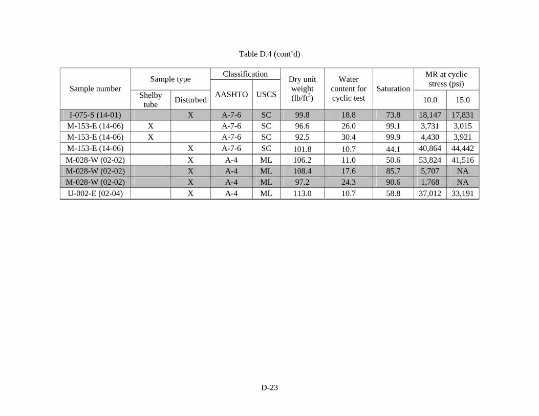
D-23
Table D.4 (cont’d)
Classification Sample type MR at cyclic stress (psi) Sample number
Shelby tube Disturbed
AASHTO USCS
Dry unit weight (lb/ft3)
Water content for cyclic test
Saturation10.0 15.0
I-075-S (14-01) X A-7-6 SC 99.8 18.8 73.8 18,147 17,831 M-153-E (14-06) X A-7-6 SC 96.6 26.0 99.1 3,731 3,015 M-153-E (14-06) X A-7-6 SC 92.5 30.4 99.9 4,430 3,921 M-153-E (14-06) X A-7-6 SC 101.8 10.7 44.1 40,864 44,442 M-028-W (02-02) X A-4 ML 106.2 11.0 50.6 53,824 41,516 M-028-W (02-02) X A-4 ML 108.4 17.6 85.7 5,707 NA M-028-W (02-02) X A-4 ML 97.2 24.3 90.6 1,768 NA U-002-E (02-04) X A-4 ML 113.0 10.7 58.8 37,012 33,191
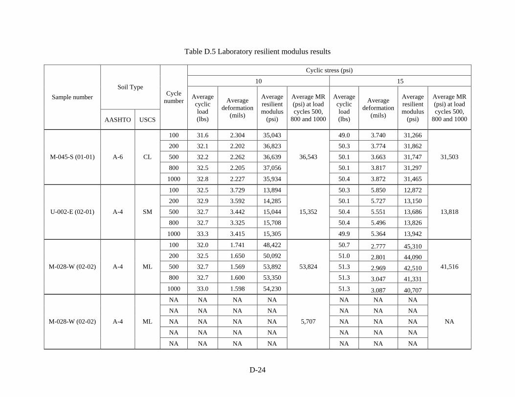
D-24
Table D.5 Laboratory resilient modulus results
Cyclic stress (psi)
10 15 Soil Type
Sample number
AASHTO USCS
Cycle number Average
cyclic load (lbs)
Average deformation
(mils)
Average resilient modulus
(psi)
Average MR (psi) at load cycles 500,
800 and 1000
Average cyclic load (lbs)
Average deformation
(mils)
Average resilient modulus
(psi)
Average MR (psi) at load cycles 500,
800 and 1000
100 31.6 2.304 35,043 49.0 3.740 31,266
200 32.1 2.202 36,823 50.3 3.774 31,862
500 32.2 2.262 36,639 50.1 3.663 31,747
800 32.5 2.205 37,056 50.1 3.817 31,297
M-045-S (01-01) A-6 CL
1000 32.8 2.227 35,934
36,543
50.4 3.872 31,465
31,503
100 32.5 3.729 13,894 50.3 5.850 12,872
200 32.9 3.592 14,285 50.1 5.727 13,150
500 32.7 3.442 15,044 50.4 5.551 13,686
800 32.7 3.325 15,708 50.4 5.496 13,826
U-002-E (02-01) A-4 SM
1000 33.3 3.415 15,305
15,352
49.9 5.364 13,942
13,818
100 32.0 1.741 48,422 50.7 2.777 45,310 200 32.5 1.650 50,092 51.0 2.801 44,090 500 32.7 1.569 53,892 51.3 2.969 42,510 800 32.7 1.600 53,350 51.3 3.047 41,331
M-028-W (02-02) A-4 ML
1000 33.0 1.598 54,230
53,824
51.3 3.087 40,707
41,516
NA NA NA NA NA NA NA
NA NA NA NA NA NA NA
NA NA NA NA NA NA NA
NA NA NA NA NA NA NA
M-028-W (02-02) A-4 ML
NA NA NA NA
5,707
NA NA NA
NA

D-25
Table D.5 (Cont’d)
Cyclic stress (psi)
10 15 Soil Type
Sample number
AASHTO USCS
Cycle number Average
cyclic load (lbs)
Average deformation
(mils)
Average resilient modulus
(psi)
Average MR (psi) at load cycles 500,
800 and 1000
Average cyclic load (lbs)
Average deformation
(mils)
Average resilient modulus (psi)
Average MR (psi) at load cycles 500,
800 and 1000
NA NA NA NA NA NA NA
NA NA NA NA NA NA NA
NA NA NA NA NA NA NA
NA NA NA NA NA NA NA
M-028-W (02-02) A-4 ML
NA NA NA NA
8,145
NA NA NA
NA
100 33.9 2.675 19,996 51.4 4.042 16,997
200 33.8 2.698 20,013 51.4 3.956 16,510
500 33.7 2.821 19,057 52.6 3.873 17,649
800 33.8 2.796 19,502 51.7 3.733 17,942
M-028-W (02-03) A-1-b SP-SM
1000 34.0 2.792 19,025
19,195
51.5 3.774 17,945
17,845
100 32.8 2.499 31,653 50.0 3.944 29,991
200 32.8 2.471 33,225 49.8 3.855 30,881
500 33.7 2.322 36,319 50.0 3.724 31,614
800 33.1 2.219 36,874 50.1 3.560 33,569
U-002-E (02-04) A-4 ML
1000 33.1 2.207 37,843
37,012
50.5 3.516 34,390
33,191
100 33.3 2.393 22,822 51.0 4.295 18,193
200 33.9 2.412 23,466 50.2 4.135 18,644
500 33.9 2.441 23,426 51.6 4.005 19,685
800 34.1 2.522 22,465 52.0 4.114 19,323
U-002-E (03-01) A-3 SP-SM
1000 34.6 2.560 22,598
22,830
51.7 3.990 19,880
19,629
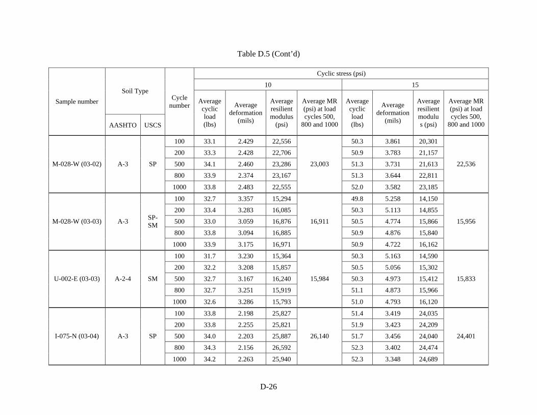
D-26
Table D.5 (Cont’d)
Cyclic stress (psi)
10 15 Soil Type
Sample number
AASHTO USCS
Cycle number Average
cyclic load (lbs)
Average deformation
(mils)
Average resilient modulus
(psi)
Average MR (psi) at load cycles 500,
800 and 1000
Average cyclic load (lbs)
Average deformation
(mils)
Average resilient modulus (psi)
Average MR (psi) at load cycles 500,
800 and 1000
100 33.1 2.429 22,556 50.3 3.861 20,301
200 33.3 2.428 22,706 50.9 3.783 21,157
500 34.1 2.460 23,286 51.3 3.731 21,613
800 33.9 2.374 23,167 51.3 3.644 22,811
M-028-W (03-02) A-3 SP
1000 33.8 2.483 22,555
23,003
52.0 3.582 23,185
22,536
100 32.7 3.357 15,294 49.8 5.258 14,150
200 33.4 3.283 16,085 50.3 5.113 14,855
500 33.0 3.059 16,876 50.5 4.774 15,866
800 33.8 3.094 16,885 50.9 4.876 15,840
M-028-W (03-03) A-3 SP-SM
1000 33.9 3.175 16,971
16,911
50.9 4.722 16,162
15,956
100 31.7 3.230 15,364 50.3 5.163 14,590
200 32.2 3.208 15,857 50.5 5.056 15,302
500 32.7 3.167 16,240 50.3 4.973 15,412
800 32.7 3.251 15,919 51.1 4.873 15,966
U-002-E (03-03) A-2-4 SM
1000 32.6 3.286 15,793
15,984
51.0 4.793 16,120
15,833
100 33.8 2.198 25,827 51.4 3.419 24,035
200 33.8 2.255 25,821 51.9 3.423 24,209
500 34.0 2.203 25,887 51.7 3.456 24,040
800 34.3 2.156 26,592 52.3 3.402 24,474
I-075-N (03-04) A-3 SP
1000 34.2 2.263 25,940
26,140
52.3 3.348 24,689
24,401

D-27
Table D.5 (cont’d)
Cyclic stress (psi)
10 15 Soil Type
Sample number
AASHTO USCS
Cycle number Average
cyclic load (lbs)
Average deformation
(mils)
Average resilient modulus
(psi)
Average MR (psi) at load cycles 500,
800 and 1000
Average cyclic load (lbs)
Average deformation
(mils)
Average resilient modulus (psi)
Average MR (psi) at load cycles 500,
800 and 1000 100 33.6 2.390 23,852 51.5 3.757 21,584
200 33.9 2.392 24,136 51.7 3.775 21,768
500 33.7 2.472 23,456 51.5 3.807 21,526
800 33.8 2.440 22,395 51.7 3.700 21,852
U-023-S (04-01) A-3 SP
1000 33.7 2.508 23,330
23,060
51.7 3.814 21,828
21,735
100 34.1 2.034 29,159 51.3 3.595 22,151
200 33.0 2.006 28,338 52.3 3.505 23,435
500 34.1 1.883 30,987 52.1 3.377 24,481
800 34.4 1.861 30,960 51.6 3.383 24,598
M-068-W (04-02) A-2-4 SC-SM
1000 34.6 1.980 30,927
30,958
51.9 3.299 25,212
24,764
100 29.4 5.139 8,572 46.6 8.078 8,440
200 30.7 4.944 9,491 47.1 7.723 8,966
500 31.3 4.879 9,725 48.6 7.368 9,822
800 31.7 4.685 10,215 48.8 7.052 10,308
M-068-W (04-03) A-3 SP
1000 31.6 4.806 9,996
9,979
48.5 7.166 9,910
10,013
100 31.7 4.463 10,722 48.7 6.850 10,728
200 31.5 4.383 10,903 49.7 6.524 11,210
500 32.1 4.101 11,945 50.0 6.427 11,637
800 32.3 4.157 11,833 50.3 6.268 11,995
M-065-S (04-04) A-2-4 SM
1000 32.5 4.190 12,050
11,943
49.6 6.038 12,096
11,909
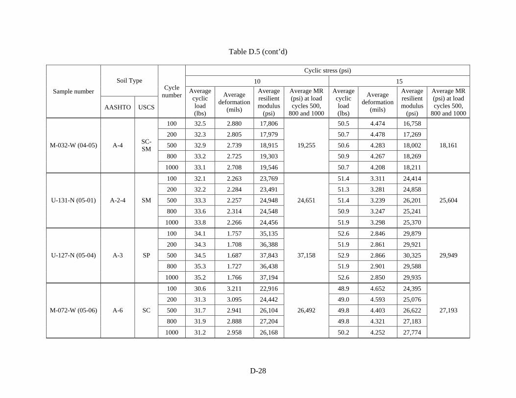
D-28
Table D.5 (cont’d)
Cyclic stress (psi)
10 15 Soil Type
Sample number
AASHTO USCS
Cycle number Average
cyclic load (lbs)
Average deformation
(mils)
Average resilient modulus
(psi)
Average MR (psi) at load cycles 500,
800 and 1000
Average cyclic load (lbs)
Average deformation
(mils)
Average resilient modulus
(psi)
Average MR (psi) at load cycles 500,
800 and 1000 100 32.5 2.880 17,806 50.5 4.474 16,758
200 32.3 2.805 17,979 50.7 4.478 17,269
500 32.9 2.739 18,915 50.6 4.283 18,002
800 33.2 2.725 19,303 50.9 4.267 18,269
M-032-W (04-05) A-4 SC-SM
1000 33.1 2.708 19,546
19,255
50.7 4.208 18,211
18,161
100 32.1 2.263 23,769 51.4 3.311 24,414
200 32.2 2.284 23,491 51.3 3.281 24,858
500 33.3 2.257 24,948 51.4 3.239 26,201
800 33.6 2.314 24,548 50.9 3.247 25,241
U-131-N (05-01) A-2-4 SM
1000 33.8 2.266 24,456
24,651
51.9 3.298 25,370
25,604
100 34.1 1.757 35,135 52.6 2.846 29,879
200 34.3 1.708 36,388 51.9 2.861 29,921
500 34.5 1.687 37,843 52.9 2.866 30,325
800 35.3 1.727 36,438 51.9 2.901 29,588
U-127-N (05-04) A-3 SP
1000 35.2 1.766 37,194
37,158
52.6 2.850 29,935
29,949
100 30.6 3.211 22,916 48.9 4.652 24,395
200 31.3 3.095 24,442 49.0 4.593 25,076
500 31.7 2.941 26,104 49.8 4.403 26,622
800 31.9 2.888 27,204 49.8 4.321 27,183
M-072-W (05-06) A-6 SC
1000 31.2 2.958 26,168
26,492
50.2 4.252 27,774
27,193
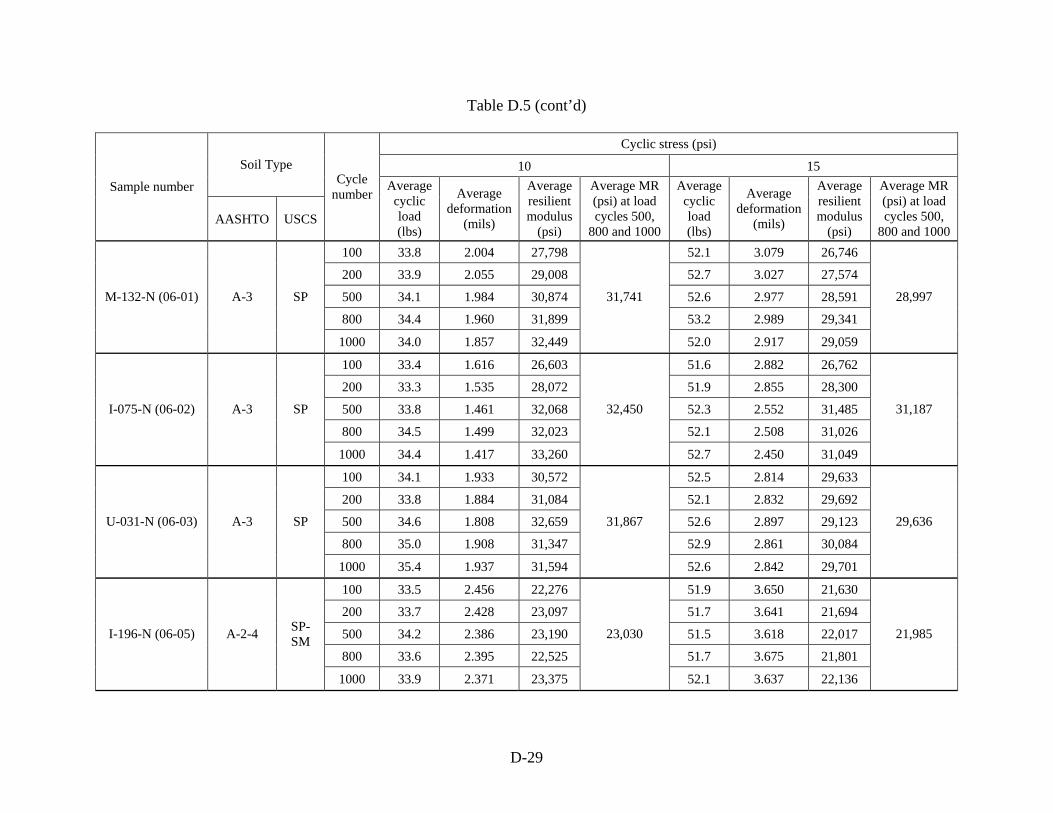
D-29
Table D.5 (cont’d)
Cyclic stress (psi)
10 15 Soil Type
Sample number
AASHTO USCS
Cycle number Average
cyclic load (lbs)
Average deformation
(mils)
Average resilient modulus
(psi)
Average MR (psi) at load cycles 500,
800 and 1000
Average cyclic load (lbs)
Average deformation
(mils)
Average resilient modulus
(psi)
Average MR (psi) at load cycles 500,
800 and 1000 100 33.8 2.004 27,798 52.1 3.079 26,746
200 33.9 2.055 29,008 52.7 3.027 27,574
500 34.1 1.984 30,874 52.6 2.977 28,591
800 34.4 1.960 31,899 53.2 2.989 29,341
M-132-N (06-01) A-3 SP
1000 34.0 1.857 32,449
31,741
52.0 2.917 29,059
28,997
100 33.4 1.616 26,603 51.6 2.882 26,762
200 33.3 1.535 28,072 51.9 2.855 28,300
500 33.8 1.461 32,068 52.3 2.552 31,485
800 34.5 1.499 32,023 52.1 2.508 31,026
I-075-N (06-02) A-3 SP
1000 34.4 1.417 33,260
32,450
52.7 2.450 31,049
31,187
100 34.1 1.933 30,572 52.5 2.814 29,633
200 33.8 1.884 31,084 52.1 2.832 29,692
500 34.6 1.808 32,659 52.6 2.897 29,123
800 35.0 1.908 31,347 52.9 2.861 30,084
U-031-N (06-03) A-3 SP
1000 35.4 1.937 31,594
31,867
52.6 2.842 29,701
29,636
100 33.5 2.456 22,276 51.9 3.650 21,630
200 33.7 2.428 23,097 51.7 3.641 21,694
500 34.2 2.386 23,190 51.5 3.618 22,017
800 33.6 2.395 22,525 51.7 3.675 21,801
I-196-N (06-05) A-2-4 SP-SM
1000 33.9 2.371 23,375
23,030
52.1 3.637 22,136
21,985
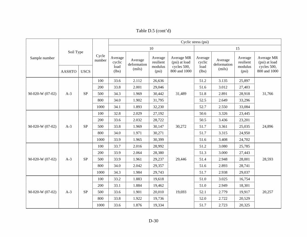
D-30
Table D.5 (cont’d)
Cyclic stress (psi)
10 15 Soil Type
Sample number
AASHTO USCS
Cycle number Average
cyclic load (lbs)
Average deformation
(mils)
Average resilient modulus
(psi)
Average MR (psi) at load cycles 500,
800 and 1000
Average cyclic load (lbs)
Average deformation
(mils)
Average resilient modulus
(psi)
Average MR (psi) at load cycles 500,
800 and 1000
100 33.6 2.112 26,636 51.2 3.135 25,897
200 33.8 2.001 29,046 51.6 3.012 27,403
500 34.3 1.969 30,442 51.8 2.891 28,918
800 34.0 1.902 31,795 52.5 2.649 33,296
M-020-W (07-02) A-3 SP
1000 34.1 1.893 32,230
31,489
52.7 2.550 33,084
31,766
100 32.8 2.029 27,192 50.6 3.326 23,445
200 33.6 2.032 28,722 50.5 3.436 23,201
500 33.8 1.969 30,147 51.7 3.361 25,035
800 34.0 1.971 30,271 51.7 3.315 24,950
M-020-W (07-02) A-3 SP
1000 33.9 1.965 30,399
30,272
51.6 3.408 24,702
24,896
100 33.7 2.016 28,992 51.2 3.080 25,785
200 33.9 2.064 28,380 51.3 3.000 27,443
500 33.9 1.961 29,237 51.4 2.948 28,001
800 34.0 2.042 29,357 51.6 2.893 28,741
M-020-W (07-02) A-3 SP
1000 34.3 1.984 29,743
29,446
51.7 2.938 29,037
28,593
100 33.2 1.883 19,618 51.0 3.025 16,754
200 33.1 1.884 19,462 51.0 2.949 18,301
500 33.6 1.901 20,010 52.1 2.779 19,917
800 33.8 1.922 19,736 52.0 2.722 20,529
M-020-W (07-02) A-3 SP
1000 33.6 1.876 19,334
19,693
51.7 2.723 20,325
20,257
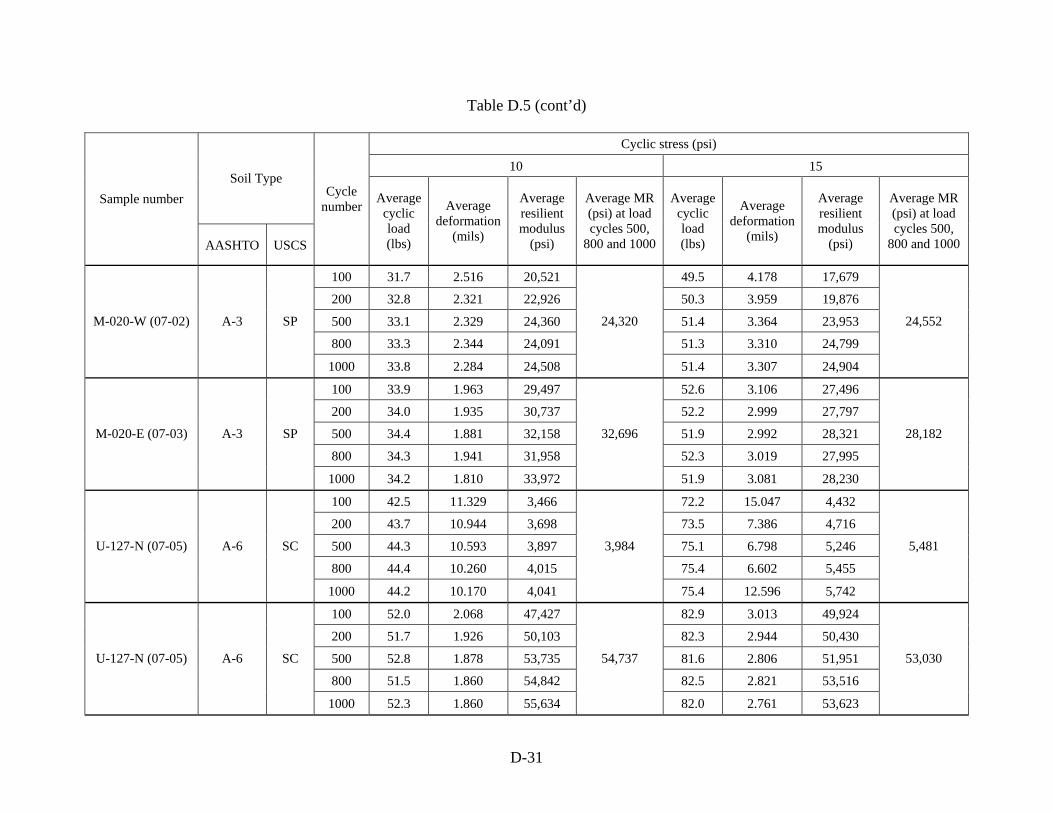
D-31
Table D.5 (cont’d)
Cyclic stress (psi)
10 15 Soil Type
Sample number
AASHTO USCS
Cycle number Average
cyclic load (lbs)
Average deformation
(mils)
Average resilient modulus
(psi)
Average MR (psi) at load cycles 500,
800 and 1000
Average cyclic load (lbs)
Average deformation
(mils)
Average resilient modulus
(psi)
Average MR (psi) at load cycles 500,
800 and 1000
100 31.7 2.516 20,521 49.5 4.178 17,679
200 32.8 2.321 22,926 50.3 3.959 19,876
500 33.1 2.329 24,360 51.4 3.364 23,953
800 33.3 2.344 24,091 51.3 3.310 24,799
M-020-W (07-02) A-3 SP
1000 33.8 2.284 24,508
24,320
51.4 3.307 24,904
24,552
100 33.9 1.963 29,497 52.6 3.106 27,496
200 34.0 1.935 30,737 52.2 2.999 27,797
500 34.4 1.881 32,158 51.9 2.992 28,321
800 34.3 1.941 31,958 52.3 3.019 27,995
M-020-E (07-03) A-3 SP
1000 34.2 1.810 33,972
32,696
51.9 3.081 28,230
28,182
100 42.5 11.329 3,466 72.2 15.047 4,432
200 43.7 10.944 3,698 73.5 7.386 4,716
500 44.3 10.593 3,897 75.1 6.798 5,246
800 44.4 10.260 4,015 75.4 6.602 5,455
U-127-N (07-05) A-6 SC
1000 44.2 10.170 4,041
3,984
75.4 12.596 5,742
5,481
100 52.0 2.068 47,427 82.9 3.013 49,924
200 51.7 1.926 50,103 82.3 2.944 50,430
500 52.8 1.878 53,735 81.6 2.806 51,951
800 51.5 1.860 54,842 82.5 2.821 53,516
U-127-N (07-05) A-6 SC
1000 52.3 1.860 55,634
54,737
82.0 2.761 53,623
53,030
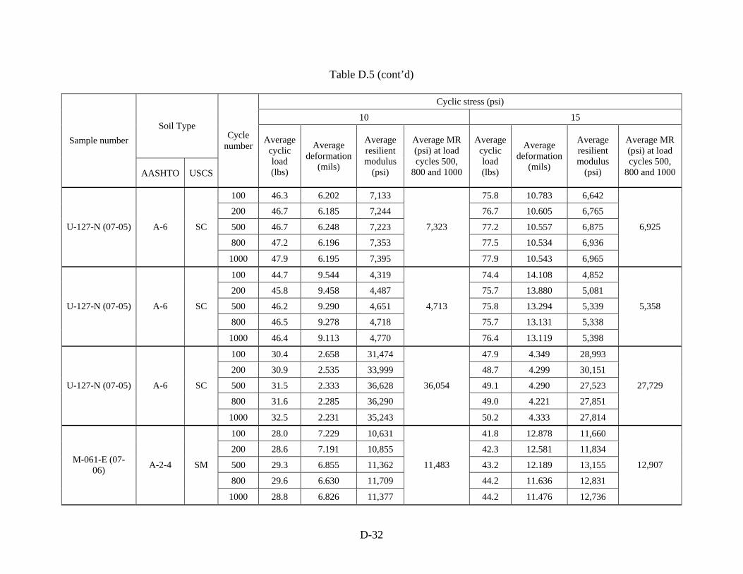
D-32
Table D.5 (cont’d)
Cyclic stress (psi)
10 15 Soil Type
Sample number
AASHTO USCS
Cycle number Average
cyclic load (lbs)
Average deformation
(mils)
Average resilient modulus
(psi)
Average MR (psi) at load cycles 500,
800 and 1000
Average cyclic load (lbs)
Average deformation
(mils)
Average resilient modulus
(psi)
Average MR (psi) at load cycles 500,
800 and 1000
100 46.3 6.202 7,133 75.8 10.783 6,642
200 46.7 6.185 7,244 76.7 10.605 6,765
500 46.7 6.248 7,223 77.2 10.557 6,875
800 47.2 6.196 7,353 77.5 10.534 6,936
U-127-N (07-05) A-6 SC
1000 47.9 6.195 7,395
7,323
77.9 10.543 6,965
6,925
100 44.7 9.544 4,319 74.4 14.108 4,852
200 45.8 9.458 4,487 75.7 13.880 5,081
500 46.2 9.290 4,651 75.8 13.294 5,339
800 46.5 9.278 4,718 75.7 13.131 5,338
U-127-N (07-05) A-6 SC
1000 46.4 9.113 4,770
4,713
76.4 13.119 5,398
5,358
100 30.4 2.658 31,474 47.9 4.349 28,993
200 30.9 2.535 33,999 48.7 4.299 30,151
500 31.5 2.333 36,628 49.1 4.290 27,523
800 31.6 2.285 36,290 49.0 4.221 27,851
U-127-N (07-05) A-6 SC
1000 32.5 2.231 35,243
36,054
50.2 4.333 27,814
27,729
100 28.0 7.229 10,631 41.8 12.878 11,660
200 28.6 7.191 10,855 42.3 12.581 11,834
500 29.3 6.855 11,362 43.2 12.189 13,155
800 29.6 6.630 11,709 44.2 11.636 12,831
M-061-E (07-06) A-2-4 SM
1000 28.8 6.826 11,377
11,483
44.2 11.476 12,736
12,907
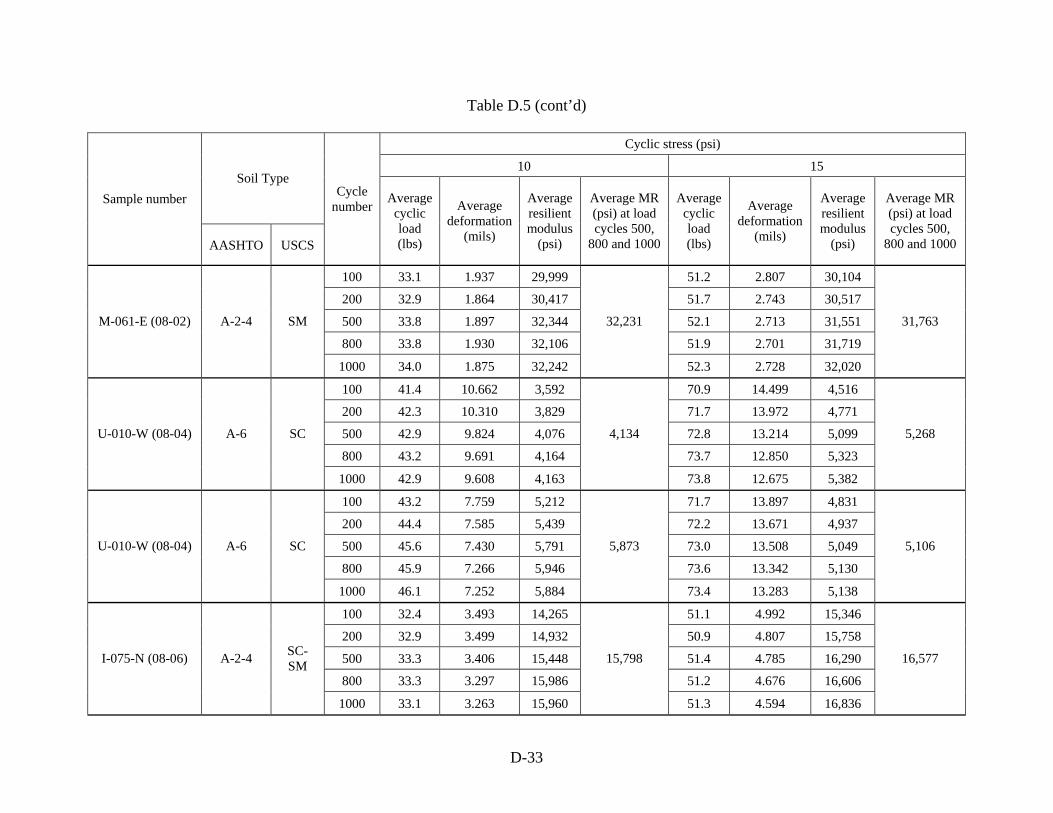
D-33
Table D.5 (cont’d)
Cyclic stress (psi)
10 15 Soil Type
Sample number
AASHTO USCS
Cycle number Average
cyclic load (lbs)
Average deformation
(mils)
Average resilient modulus
(psi)
Average MR (psi) at load cycles 500,
800 and 1000
Average cyclic load (lbs)
Average deformation
(mils)
Average resilient modulus
(psi)
Average MR (psi) at load cycles 500,
800 and 1000
100 33.1 1.937 29,999 51.2 2.807 30,104
200 32.9 1.864 30,417 51.7 2.743 30,517
500 33.8 1.897 32,344 52.1 2.713 31,551
800 33.8 1.930 32,106 51.9 2.701 31,719
M-061-E (08-02) A-2-4 SM
1000 34.0 1.875 32,242
32,231
52.3 2.728 32,020
31,763
100 41.4 10.662 3,592 70.9 14.499 4,516
200 42.3 10.310 3,829 71.7 13.972 4,771
500 42.9 9.824 4,076 72.8 13.214 5,099
800 43.2 9.691 4,164 73.7 12.850 5,323
U-010-W (08-04) A-6 SC
1000 42.9 9.608 4,163
4,134
73.8 12.675 5,382
5,268
100 43.2 7.759 5,212 71.7 13.897 4,831
200 44.4 7.585 5,439 72.2 13.671 4,937
500 45.6 7.430 5,791 73.0 13.508 5,049
800 45.9 7.266 5,946 73.6 13.342 5,130
U-010-W (08-04) A-6 SC
1000 46.1 7.252 5,884
5,873
73.4 13.283 5,138
5,106
100 32.4 3.493 14,265 51.1 4.992 15,346
200 32.9 3.499 14,932 50.9 4.807 15,758
500 33.3 3.406 15,448 51.4 4.785 16,290
800 33.3 3.297 15,986 51.2 4.676 16,606
I-075-N (08-06) A-2-4 SC-SM
1000 33.1 3.263 15,960
15,798
51.3 4.594 16,836
16,577
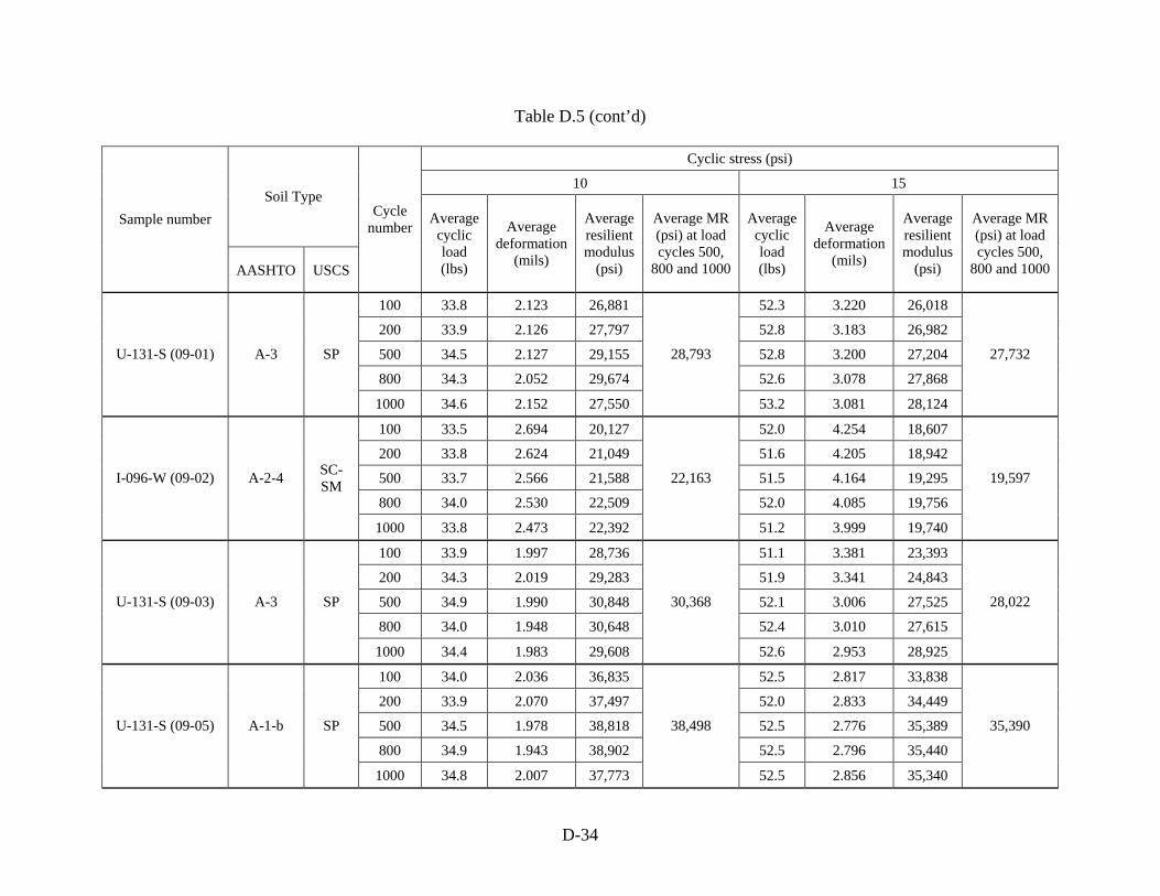
D-34
Table D.5 (cont’d)
Cyclic stress (psi)
10 15 Soil Type
Sample number
AASHTO USCS
Cycle number Average
cyclic load (lbs)
Average deformation
(mils)
Average resilient modulus
(psi)
Average MR (psi) at load cycles 500,
800 and 1000
Average cyclic load (lbs)
Average deformation
(mils)
Average resilient modulus
(psi)
Average MR (psi) at load cycles 500,
800 and 1000
100 33.8 2.123 26,881 52.3 3.220 26,018
200 33.9 2.126 27,797 52.8 3.183 26,982
500 34.5 2.127 29,155 52.8 3.200 27,204
800 34.3 2.052 29,674 52.6 3.078 27,868
U-131-S (09-01) A-3 SP
1000 34.6 2.152 27,550
28,793
53.2 3.081 28,124
27,732
100 33.5 2.694 20,127 52.0 4.254 18,607
200 33.8 2.624 21,049 51.6 4.205 18,942
500 33.7 2.566 21,588 51.5 4.164 19,295
800 34.0 2.530 22,509 52.0 4.085 19,756
I-096-W (09-02) A-2-4 SC-SM
1000 33.8 2.473 22,392
22,163
51.2 3.999 19,740
19,597
100 33.9 1.997 28,736 51.1 3.381 23,393
200 34.3 2.019 29,283 51.9 3.341 24,843
500 34.9 1.990 30,848 52.1 3.006 27,525
800 34.0 1.948 30,648 52.4 3.010 27,615
U-131-S (09-03) A-3 SP
1000 34.4 1.983 29,608
30,368
52.6 2.953 28,925
28,022
100 34.0 2.036 36,835 52.5 2.817 33,838
200 33.9 2.070 37,497 52.0 2.833 34,449
500 34.5 1.978 38,818 52.5 2.776 35,389
800 34.9 1.943 38,902 52.5 2.796 35,440
U-131-S (09-05) A-1-b SP
1000 34.8 2.007 37,773
38,498
52.5 2.856 35,340
35,390

D-35
Table D.5 (cont’d)
Cyclic stress (psi)
10 15 Soil Type
Sample number
AASHTO USCS
Cycle number Average
cyclic load (lbs)
Average deformation
(mils)
Average resilient modulus
(psi)
Average MR (psi) at load cycles 500,
800 and 1000
Average cyclic load (lbs)
Average deformation
(mils)
Average resilient modulus
(psi)
Average MR (psi) at load cycles 500,
800 and 1000
100 33.4 2.943 17,969 51.4 4.275 18,433
200 33.5 2.928 18,261 52.0 4.175 19,068
500 33.9 2.948 18,534 51.6 4.086 19,511
800 33.7 2.841 18,744 51.6 4.043 19,663
M-044-E (09-07) A-2-4 SM
1000 34.0 3.046 18,023
18,434
51.9 4.041 19,788
19,654
100 33.1 3.415 15,148 50.4 5.279 14,639
200 33.1 3.421 15,097 50.5 5.143 15,004
500 33.6 3.458 15,204 50.6 4.889 15,786
800 32.9 3.427 14,945 50.8 4.853 15,880
M-024-S (09-09) A-2-4 SM
1000 33.3 3.378 15,318
15,156
51.0 4.891 15,897
15,854
100 34.0 1.985 29,263 52.2 3.321 25,428
200 34.1 2.074 29,172 52.2 3.248 25,709
500 34.4 2.071 28,746 52.3 3.163 26,255
800 34.3 2.079 29,232 51.9 3.231 25,802
I-069-E (09-10) A-3 SP
1000 34.8 2.160 28,012
28,663
52.4 3.192 26,227
26,095
100 33.5 3.483 14,917 51.2 4.732 16,473
200 33.5 3.542 14,864 51.1 4.694 16,512
500 33.1 3.344 15,551 51.3 4.485 17,528
800 33.8 3.457 15,312 50.8 4.533 17,144
I-069-N (10-01) A-3 SP-SM
1000 34.0 3.162 16,756
15,873
51.7 4.526 17,509
17,394
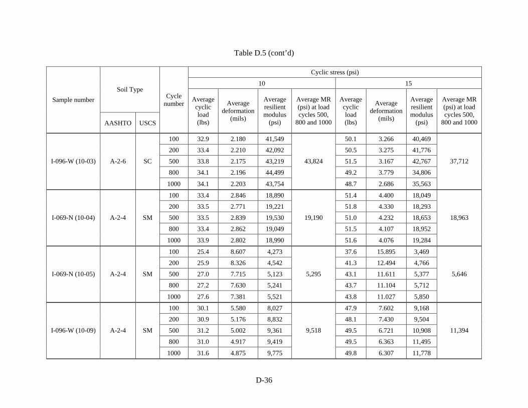
D-36
Table D.5 (cont’d)
Cyclic stress (psi)
10 15 Soil Type
Sample number
AASHTO USCS
Cycle number Average
cyclic load (lbs)
Average deformation
(mils)
Average resilient modulus
(psi)
Average MR (psi) at load cycles 500,
800 and 1000
Average cyclic load (lbs)
Average deformation
(mils)
Average resilient modulus
(psi)
Average MR (psi) at load cycles 500,
800 and 1000
100 32.9 2.180 41,549 50.1 3.266 40,469
200 33.4 2.210 42,092 50.5 3.275 41,776
500 33.8 2.175 43,219 51.5 3.167 42,767
800 34.1 2.196 44,499 49.2 3.779 34,806
I-096-W (10-03) A-2-6 SC
1000 34.1 2.203 43,754
43,824
48.7 2.686 35,563
37,712
100 33.4 2.846 18,890 51.4 4.400 18,049
200 33.5 2.771 19,221 51.8 4.330 18,293
500 33.5 2.839 19,530 51.0 4.232 18,653
800 33.4 2.862 19,049 51.5 4.107 18,952
I-069-N (10-04) A-2-4 SM
1000 33.9 2.802 18,990
19,190
51.6 4.076 19,284
18,963
100 25.4 8.607 4,273 37.6 15.895 3,469
200 25.9 8.326 4,542 41.3 12.494 4,766
500 27.0 7.715 5,123 43.1 11.611 5,377
800 27.2 7.630 5,241 43.7 11.104 5,712
I-069-N (10-05) A-2-4 SM
1000 27.6 7.381 5,521
5,295
43.8 11.027 5,850
5,646
100 30.1 5.580 8,027 47.9 7.602 9,168
200 30.9 5.176 8,832 48.1 7.430 9,504
500 31.2 5.002 9,361 49.5 6.721 10,908
800 31.0 4.917 9,419 49.5 6.363 11,495
I-096-W (10-09) A-2-4 SM
1000 31.6 4.875 9,775
9,518
49.8 6.307 11,778
11,394
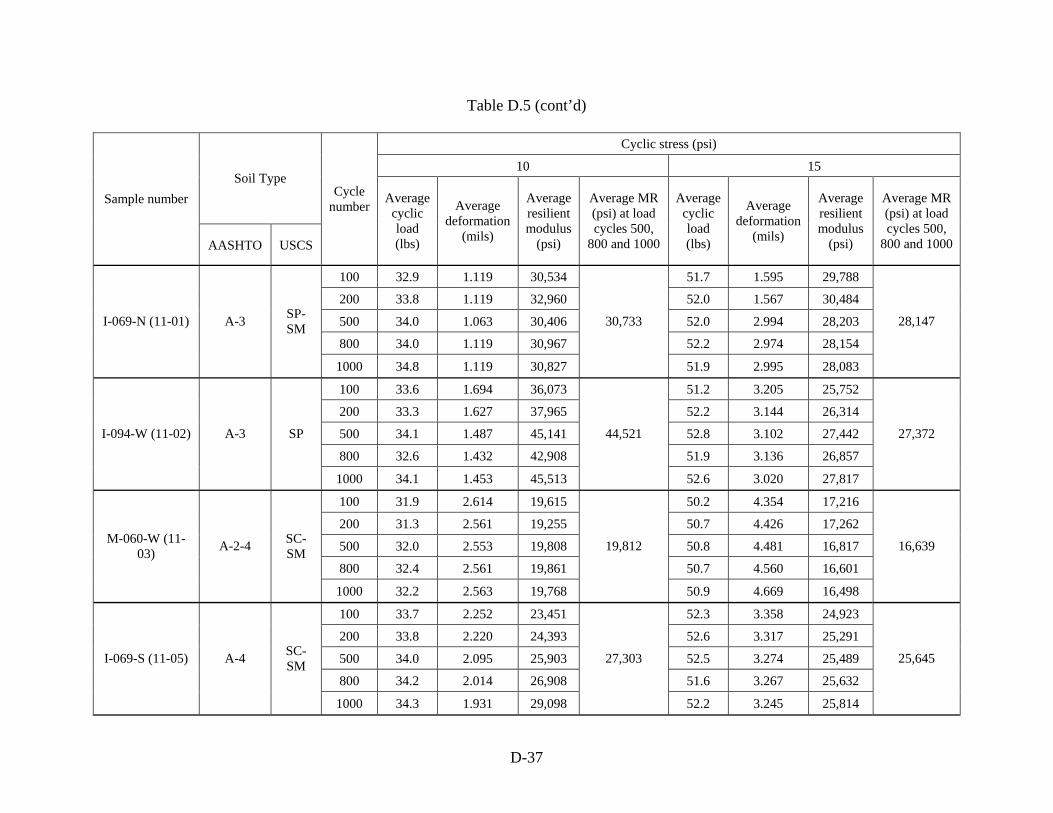
D-37
Table D.5 (cont’d)
Cyclic stress (psi)
10 15 Soil Type
Sample number
AASHTO USCS
Cycle number Average
cyclic load (lbs)
Average deformation
(mils)
Average resilient modulus
(psi)
Average MR (psi) at load cycles 500,
800 and 1000
Average cyclic load (lbs)
Average deformation
(mils)
Average resilient modulus
(psi)
Average MR (psi) at load cycles 500,
800 and 1000
100 32.9 1.119 30,534 51.7 1.595 29,788
200 33.8 1.119 32,960 52.0 1.567 30,484
500 34.0 1.063 30,406 52.0 2.994 28,203
800 34.0 1.119 30,967 52.2 2.974 28,154
I-069-N (11-01) A-3 SP-SM
1000 34.8 1.119 30,827
30,733
51.9 2.995 28,083
28,147
100 33.6 1.694 36,073 51.2 3.205 25,752
200 33.3 1.627 37,965 52.2 3.144 26,314
500 34.1 1.487 45,141 52.8 3.102 27,442
800 32.6 1.432 42,908 51.9 3.136 26,857
I-094-W (11-02) A-3 SP
1000 34.1 1.453 45,513
44,521
52.6 3.020 27,817
27,372
100 31.9 2.614 19,615 50.2 4.354 17,216
200 31.3 2.561 19,255 50.7 4.426 17,262
500 32.0 2.553 19,808 50.8 4.481 16,817
800 32.4 2.561 19,861 50.7 4.560 16,601
M-060-W (11-03) A-2-4 SC-
SM
1000 32.2 2.563 19,768
19,812
50.9 4.669 16,498
16,639
100 33.7 2.252 23,451 52.3 3.358 24,923
200 33.8 2.220 24,393 52.6 3.317 25,291
500 34.0 2.095 25,903 52.5 3.274 25,489
800 34.2 2.014 26,908 51.6 3.267 25,632
I-069-S (11-05) A-4 SC-SM
1000 34.3 1.931 29,098
27,303
52.2 3.245 25,814
25,645
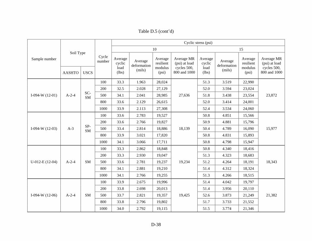
D-38
Table D.5 (cont’d)
Cyclic stress (psi)
10 15 Soil Type
Sample number
AASHTO USCS
Cycle number Average
cyclic load (lbs)
Average deformation
(mils)
Average resilient modulus
(psi)
Average MR (psi) at load cycles 500,
800 and 1000
Average cyclic load (lbs)
Average deformation
(mils)
Average resilient modulus
(psi)
Average MR (psi) at load cycles 500,
800 and 1000
100 33.3 1.963 28,024 51.3 3.519 22,990
200 32.5 2.028 27,129 52.0 3.594 23,024
500 34.1 2.041 28,985 51.8 3.438 23,554
800 33.6 2.129 26,615 52.0 3.414 24,001
I-094-W (12-01) A-2-4 SC-SM
1000 33.9 2.113 27,308
27,636
52.4 3.534 24,060
23,872
100 33.6 2.783 19,527 50.8 4.851 15,566
200 33.6 2.766 19,827 50.9 4.881 15,796
500 33.4 2.814 18,886 50.4 4.789 16,090
800 33.9 3.021 17,820 50.8 4.831 15,893
I-094-W (12-03) A-3 SP-SM
1000 34.1 3.066 17,711
18,139
50.8 4.798 15,947
15,977
100 33.3 2.862 18,848 50.8 4.340 18,416
200 33.3 2.930 19,047 51.3 4.323 18,683
500 33.6 2.781 19,237 51.2 4.264 18,191
800 34.1 2.881 19,210 51.4 4.312 18,324
U-012-E (12-04) A-2-4 SM
1000 34.1 2.766 19,255
19,234
51.3 4.266 18,515
18,343
100 33.9 2.675 19,996 51.4 4.042 19,797
200 33.8 2.698 20,013 51.4 3.956 20,110
500 33.7 2.821 19,357 52.6 3.873 21,249
800 33.8 2.796 19,802 51.7 3.733 21,552
I-094-W (12-06) A-2-4 SM
1000 34.0 2.792 19,115
19,425
51.5 3.774 21,346
21,382

D-39
Table D.5 (cont’d)
Cyclic stress (psi)
10 15 Soil Type
Sample number
AASHTO USCS
Cycle number Average
cyclic load (lbs)
Average deformation
(mils)
Average resilient modulus
(psi)
Average MR (psi) at load cycles 500,
800 and 1000
Average cyclic load (lbs)
Average deformation
(mils)
Average resilient modulus
(psi)
Average MR (psi) at load cycles 500,
800 and 1000
NA NA NA NA NA NA NA
NA NA NA NA NA NA NA
NA NA NA NA NA NA NA
NA NA NA NA NA NA NA
I-094-W (12-06) A-2-4 SM
NA NA NA NA
9,610
NA NA NA
NA
10 psi 13 psi 18 psi 21 psi
I-094-W (12-06) A-2-4 SM 13,363 12,463
NA 11,233 10,929
100 34.4 3.172 17,093 51.9 5.000 15,746
200 34.0 3.101 17,359 50.0 4.846 15,814
500 34.8 3.149 17,853 51.5 4.878 16,213
800 34.6 3.049 17,891 51.6 4.844 16,042
M-024-S (13-01) A-4 SM
1000 35.1 3.052 18,106
17,950
51.8 4.844 16,271
16,175
100 33.6 2.042 28,216 51.7 3.362 23,959
200 33.5 2.112 27,648 51.9 3.351 24,234
500 33.9 2.186 26,464 52.1 3.478 23,699
800 33.9 2.368 24,623 51.7 3.453 23,882
M-059-W (13-02) A-3 SP
1000 33.8 2.439 23,502
24,863
51.9 3.436 23,849
23,810
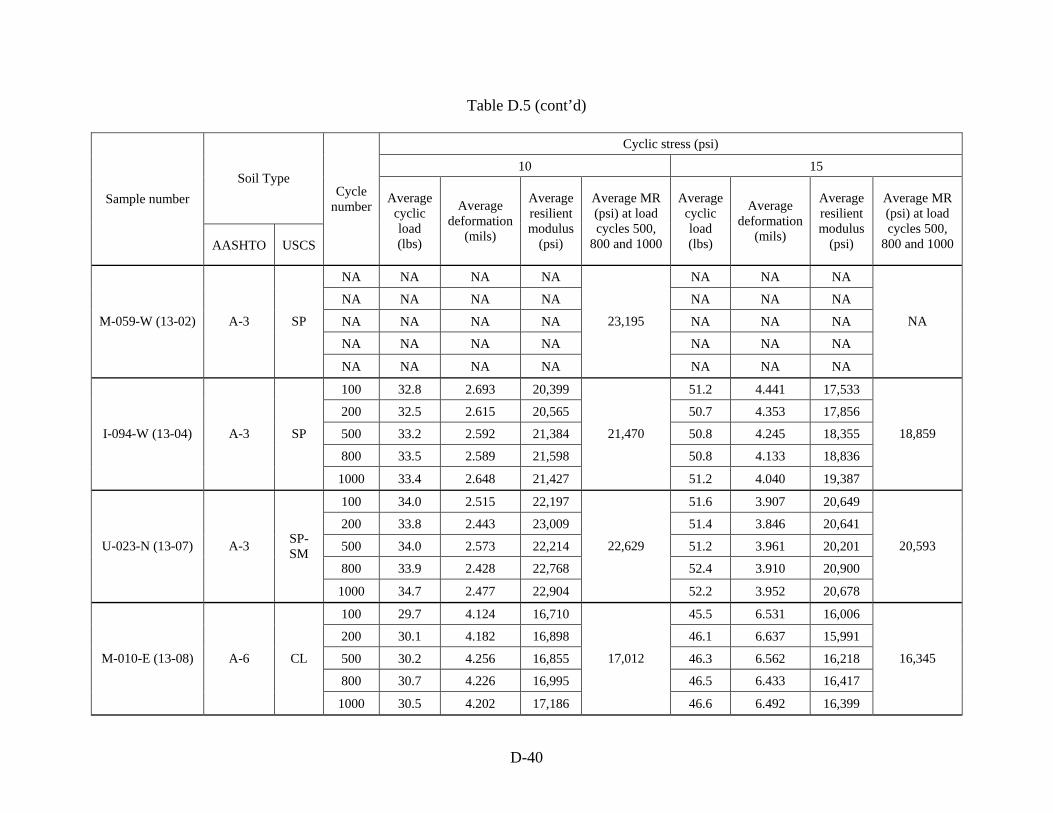
D-40
Table D.5 (cont’d)
Cyclic stress (psi)
10 15 Soil Type
Sample number
AASHTO USCS
Cycle number Average
cyclic load (lbs)
Average deformation
(mils)
Average resilient modulus
(psi)
Average MR (psi) at load cycles 500,
800 and 1000
Average cyclic load (lbs)
Average deformation
(mils)
Average resilient modulus
(psi)
Average MR (psi) at load cycles 500,
800 and 1000
NA NA NA NA NA NA NA
NA NA NA NA NA NA NA
NA NA NA NA NA NA NA
NA NA NA NA NA NA NA
M-059-W (13-02) A-3 SP
NA NA NA NA
23,195
NA NA NA
NA
100 32.8 2.693 20,399 51.2 4.441 17,533
200 32.5 2.615 20,565 50.7 4.353 17,856
500 33.2 2.592 21,384 50.8 4.245 18,355
800 33.5 2.589 21,598 50.8 4.133 18,836
I-094-W (13-04) A-3 SP
1000 33.4 2.648 21,427
21,470
51.2 4.040 19,387
18,859
100 34.0 2.515 22,197 51.6 3.907 20,649
200 33.8 2.443 23,009 51.4 3.846 20,641
500 34.0 2.573 22,214 51.2 3.961 20,201
800 33.9 2.428 22,768 52.4 3.910 20,900
U-023-N (13-07) A-3 SP-SM
1000 34.7 2.477 22,904
22,629
52.2 3.952 20,678
20,593
100 29.7 4.124 16,710 45.5 6.531 16,006
200 30.1 4.182 16,898 46.1 6.637 15,991
500 30.2 4.256 16,855 46.3 6.562 16,218
800 30.7 4.226 16,995 46.5 6.433 16,417
M-010-E (13-08) A-6 CL
1000 30.5 4.202 17,186
17,012
46.6 6.492 16,399
16,345

D-41
Table D.5 (cont’d)
Cyclic stress (psi)
10 15 Soil Type
Sample number
AASHTO USCS
Cycle number Average
cyclic load (lbs)
Average deformation
(mils)
Average resilient modulus
(psi)
Average MR (psi) at load cycles 500,
800 and 1000
Average cyclic load (lbs)
Average deformation
(mils)
Average resilient modulus
(psi)
Average MR (psi) at load cycles 500,
800 and 1000
100 48.6 3.375 14,374 77.7 7.441 9,934
200 49.6 3.334 15,053 78.1 7.453 9,867
500 49.6 3.271 15,423 78.2 7.743 9,627
800 49.8 3.258 15,631 78.2 7.779 9,528
M-010-E (13-08) A-6 CL
1000 49.8 3.257 15,629
15,561
78.3 7.849 9,504
9,553
100 51.5 1.331 31,968 83.3 1.796 36,929
200 51.8 1.291 36,534 82.8 1.731 38,488
500 52.7 1.218 43,564 82.5 1.808 40,155
800 52.3 1.211 45,089 82.2 1.629 42,399
M-010-E (13-08) A-6 CL
1000 51.8 1.152 45,271
44,641
82.4 1.793 43,414
41,989
100 39.6 7.658 8,407 46.6 8.078 8,440
200 41.3 7.157 9,399 47.1 7.723 8,966
500 42.2 6.971 9,004 48.6 7.368 8,822
800 43.5 6.473 9,818 48.8 7.052 8,108
M-010-E (13-08) A-6 CL
1000 44.0 6.376 10,317
9,713
48.5 7.166 7,910
8,280
100 30.3 2.283 11,369 48.9 3.899 14,813
200 31.0 2.259 13,560 48.7 3.804 15,893
500 31.3 2.074 17,389 48.9 3.721 16,938
800 31.7 1.971 18,449 49.6 3.586 18,253
I-075-S (14-01) A-7-6 SC
1000 32.0 2.067 18,825
18,221
49.6 3.573 18,336
17,842
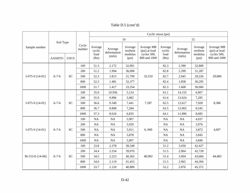
D-42
Table D.5 (cont’d)
Cyclic stress (psi)
10 15 Soil Type
Sample number
AASHTO USCS
Cycle number Average
cyclic load (lbs)
Average deformation
(mils)
Average resilient modulus
(psi)
Average MR (psi) at load cycles 500,
800 and 1000
Average cyclic load (lbs)
Average deformation
(mils)
Average resilient modulus
(psi)
Average MR (psi) at load cycles 500,
800 and 1000
100 51.3 2.172 32,901 82.3 2.390 32,808
200 51.2 1.994 36,098 82.8 2.299 31,287
500 52.3 1.815 31,799 82.7 2.045 29,226
800 52.3 1.481 32,377 82.4 1.858 30,295
I-075-S (14-01) A-7-6 SC
1000 51.7 1.417 33,354
32,510
82.3 1.668 30,060
29,860
100 35.0 10.936 5,114 61.1 14.155 6,907
200 35.9 9.896 5,982 61.6 13.624 7,285
500 36.6 9.349 7,441 62.5 12.617 7,928
800 36.7 8.808 7,284 63.5 12.002 8,545
I-075-S (14-01) A-7-6 SC
1000 37.3 8.616 6,835
7,187
64.1 11.896 8,685
8,386
100 NA NA 5,907 NA NA 4,037
200 NA NA 5,929 NA NA 3,976
500 NA NA 5,911 NA NA 3,872
800 NA NA 5,878 NA NA 3,845
I-075-S (14-01) A-7-6 SC
1000 NA NA 5,907
6, 069
NA NA 3,846
4,007
100 33.8 2.378 38,348 51.2 3.050 42,427
200 34.4 2.254 39,970 51.5 2.964 42,728
500 34.5 2.223 40,365 51.4 3.004 43,684
800 34.0 2.119 41,453 51.5 2.965 44,394
M-153-E (14-06) A-7-6 SC
1000 33.7 2.120 40,889
40,902
52.2 2.876 45,372
44,483
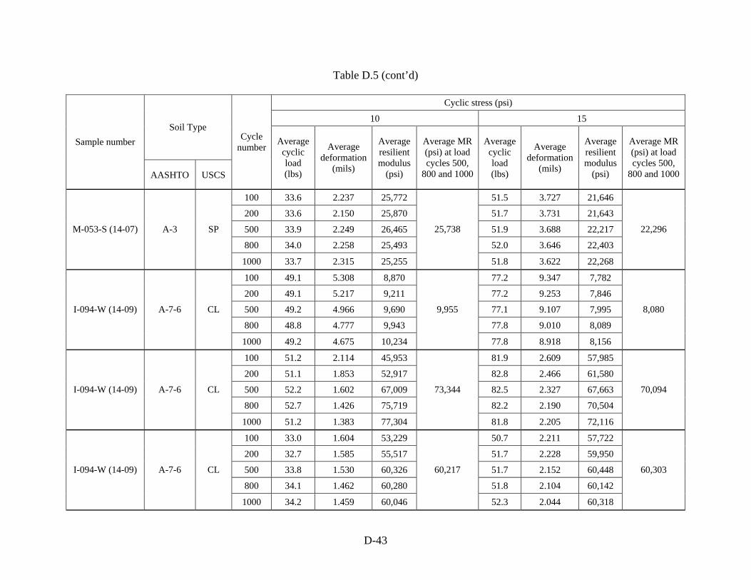
D-43
Table D.5 (cont’d)
Cyclic stress (psi)
10 15 Soil Type
Sample number
AASHTO USCS
Cycle number Average
cyclic load (lbs)
Average deformation
(mils)
Average resilient modulus
(psi)
Average MR (psi) at load cycles 500,
800 and 1000
Average cyclic load (lbs)
Average deformation
(mils)
Average resilient modulus
(psi)
Average MR (psi) at load cycles 500,
800 and 1000
100 33.6 2.237 25,772 51.5 3.727 21,646
200 33.6 2.150 25,870 51.7 3.731 21,643
500 33.9 2.249 26,465 51.9 3.688 22,217
800 34.0 2.258 25,493 52.0 3.646 22,403
M-053-S (14-07) A-3 SP
1000 33.7 2.315 25,255
25,738
51.8 3.622 22,268
22,296
100 49.1 5.308 8,870 77.2 9.347 7,782
200 49.1 5.217 9,211 77.2 9.253 7,846
500 49.2 4.966 9,690 77.1 9.107 7,995
800 48.8 4.777 9,943 77.8 9.010 8,089
I-094-W (14-09) A-7-6 CL
1000 49.2 4.675 10,234
9,955
77.8 8.918 8,156
8,080
100 51.2 2.114 45,953 81.9 2.609 57,985
200 51.1 1.853 52,917 82.8 2.466 61,580
500 52.2 1.602 67,009 82.5 2.327 67,663
800 52.7 1.426 75,719 82.2 2.190 70,504
I-094-W (14-09) A-7-6 CL
1000 51.2 1.383 77,304
73,344
81.8 2.205 72,116
70,094
100 33.0 1.604 53,229 50.7 2.211 57,722
200 32.7 1.585 55,517 51.7 2.228 59,950
500 33.8 1.530 60,326 51.7 2.152 60,448
800 34.1 1.462 60,280 51.8 2.104 60,142
I-094-W (14-09) A-7-6 CL
1000 34.2 1.459 60,046
60,217
52.3 2.044 60,318
60,303
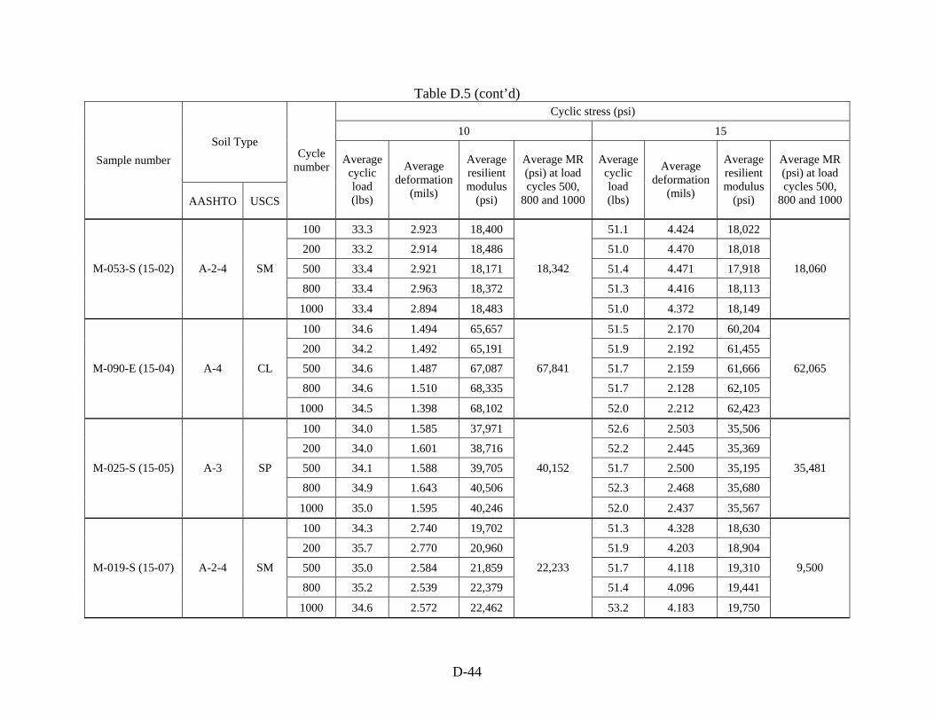
D-44
Table D.5 (cont’d) Cyclic stress (psi)
10 15 Soil Type
Sample number
AASHTO USCS
Cycle number Average
cyclic load (lbs)
Average deformation
(mils)
Average resilient modulus
(psi)
Average MR (psi) at load cycles 500,
800 and 1000
Average cyclic load (lbs)
Average deformation
(mils)
Average resilient modulus
(psi)
Average MR (psi) at load cycles 500,
800 and 1000
100 33.3 2.923 18,400 51.1 4.424 18,022
200 33.2 2.914 18,486 51.0 4.470 18,018
500 33.4 2.921 18,171 51.4 4.471 17,918
800 33.4 2.963 18,372 51.3 4.416 18,113
M-053-S (15-02) A-2-4 SM
1000 33.4 2.894 18,483
18,342
51.0 4.372 18,149
18,060
100 34.6 1.494 65,657 51.5 2.170 60,204
200 34.2 1.492 65,191 51.9 2.192 61,455
500 34.6 1.487 67,087 51.7 2.159 61,666
800 34.6 1.510 68,335 51.7 2.128 62,105
M-090-E (15-04) A-4 CL
1000 34.5 1.398 68,102
67,841
52.0 2.212 62,423
62,065
100 34.0 1.585 37,971 52.6 2.503 35,506
200 34.0 1.601 38,716 52.2 2.445 35,369
500 34.1 1.588 39,705 51.7 2.500 35,195
800 34.9 1.643 40,506 52.3 2.468 35,680
M-025-S (15-05) A-3 SP
1000 35.0 1.595 40,246
40,152
52.0 2.437 35,567
35,481
100 34.3 2.740 19,702 51.3 4.328 18,630
200 35.7 2.770 20,960 51.9 4.203 18,904
500 35.0 2.584 21,859 51.7 4.118 19,310
800 35.2 2.539 22,379 51.4 4.096 19,441
M-019-S (15-07) A-2-4 SM
1000 34.6 2.572 22,462
22,233
53.2 4.183 19,750
9,500

E-1
APPENDIX E
FWD RESULTS
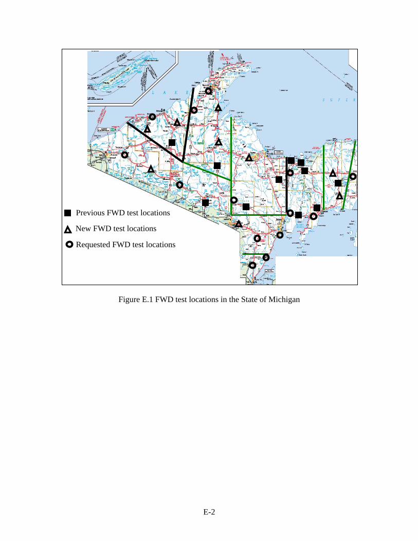
E-2
Figure E.1 FWD test locations in the State of Michigan
Previous FWD test locations
Requested FWD test locations
New FWD test locations
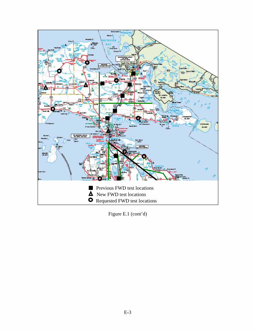
E-3
Figure E.1 (cont’d)
Previous FWD test locations
Requested FWD test locations New FWD test locations
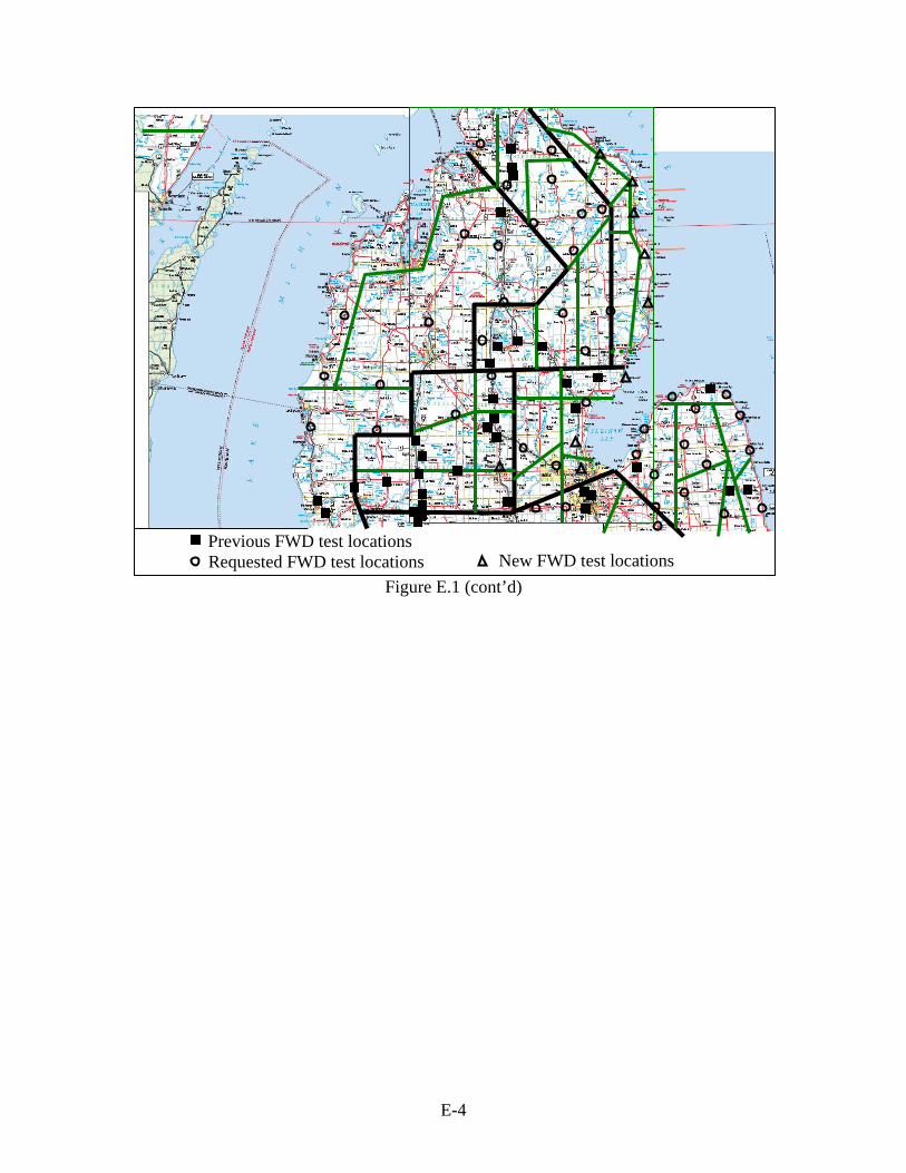
E-4
Figure E.1 (cont’d)
Previous FWD test locations Requested FWD test locations New FWD test locations
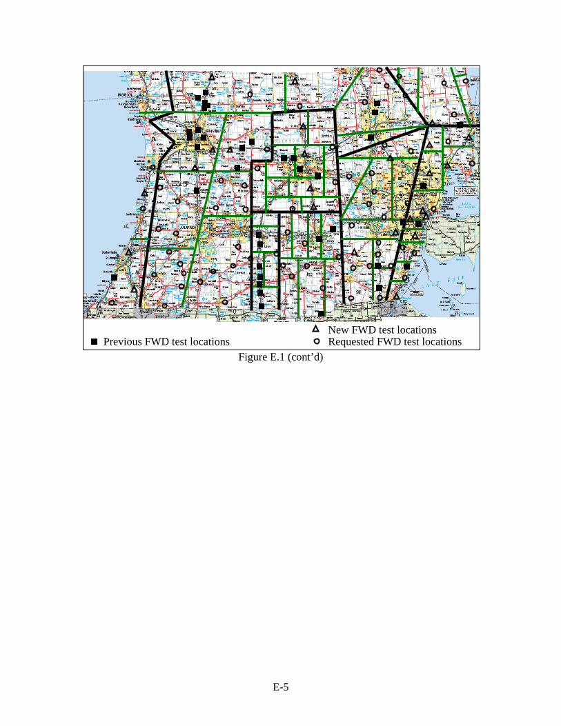
E-5
Figure E.1 (cont’d)
Previous FWD test locations Requested FWD test locations New FWD test locations
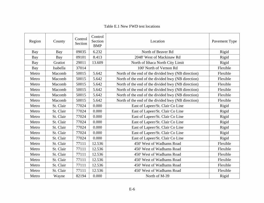
E-6
Table E.1 New FWD test locations
Region County Control Section
Control Section BMP
Location Pavement Type
Bay Bay 09035 6.232 North of Beaver Rd Rigid Bay Bay 09101 8.413 2048' West of Mackinaw Rd Rigid Bay Gratiot 29011 13.609 North of Ithaca North City Limit Rigid Bay Isabella 37014 100' North of Vernon Rd Flexible
Metro Macomb 50015 5.642 North of the end of the divided hwy (NB direction) Flexible Metro Macomb 50015 5.642 North of the end of the divided hwy (NB direction) Flexible Metro Macomb 50015 5.642 North of the end of the divided hwy (NB direction) Flexible Metro Macomb 50015 5.642 North of the end of the divided hwy (NB direction) Flexible Metro Macomb 50015 5.642 North of the end of the divided hwy (NB direction) Flexible Metro Macomb 50015 5.642 North of the end of the divided hwy (NB direction) Flexible Metro St. Clair 77024 0.000 East of Lapeer/St. Clair Co Line Rigid Metro St. Clair 77024 0.000 East of Lapeer/St. Clair Co Line Rigid Metro St. Clair 77024 0.000 East of Lapeer/St. Clair Co Line Rigid Metro St. Clair 77024 0.000 East of Lapeer/St. Clair Co Line Rigid Metro St. Clair 77024 0.000 East of Lapeer/St. Clair Co Line Rigid Metro St. Clair 77024 0.000 East of Lapeer/St. Clair Co Line Rigid Metro St. Clair 77024 0.000 East of Lapeer/St. Clair Co Line Rigid Metro St. Clair 77111 12.536 450' West of Wadhams Road Flexible Metro St. Clair 77111 12.536 450' West of Wadhams Road Flexible Metro St. Clair 77111 12.536 450' West of Wadhams Road Flexible Metro St. Clair 77111 12.536 450' West of Wadhams Road Flexible Metro St. Clair 77111 12.536 450' West of Wadhams Road Flexible Metro St. Clair 77111 12.536 450' West of Wadhams Road Flexible Metro Wayne 82194 0.000 North of M-39 Rigid
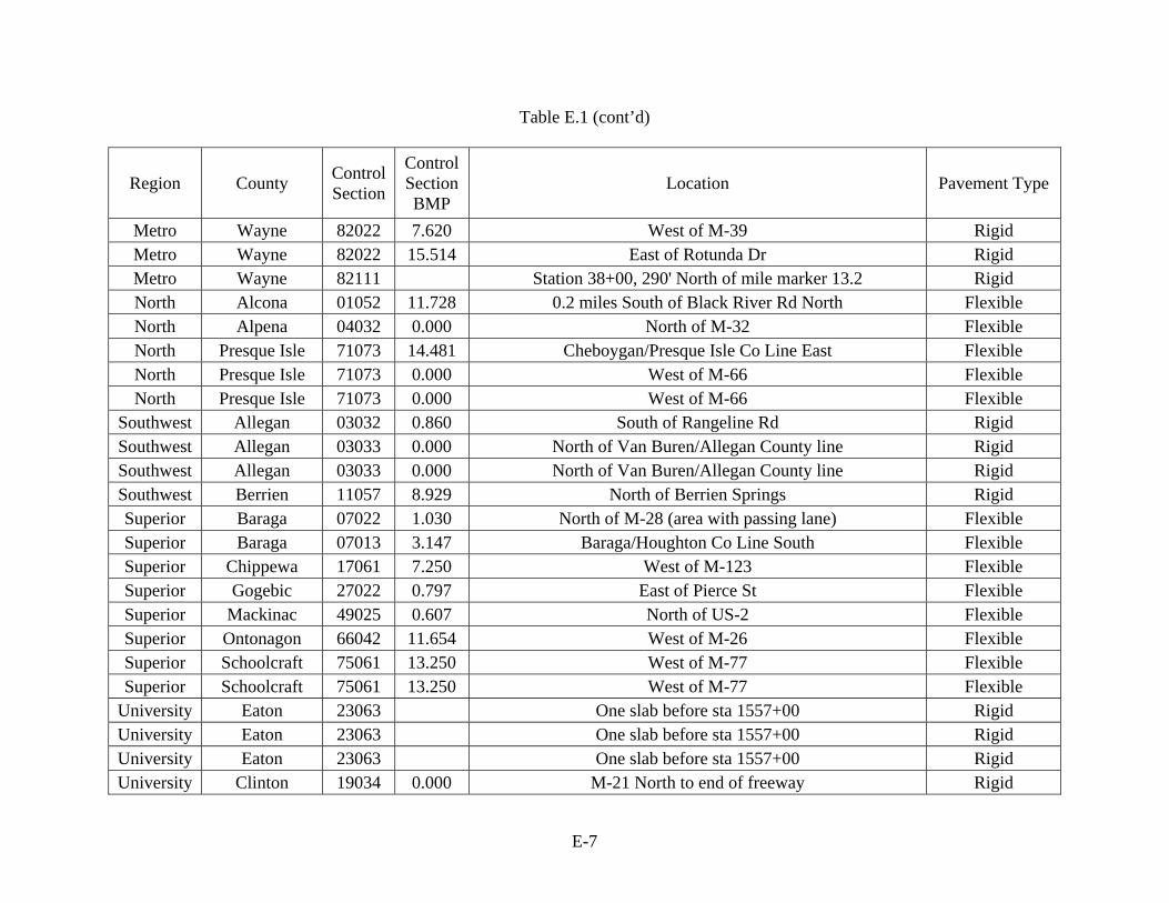
E-7
Table E.1 (cont’d)
Region County Control Section
Control Section BMP
Location Pavement Type
Metro Wayne 82022 7.620 West of M-39 Rigid Metro Wayne 82022 15.514 East of Rotunda Dr Rigid Metro Wayne 82111 Station 38+00, 290' North of mile marker 13.2 Rigid North Alcona 01052 11.728 0.2 miles South of Black River Rd North Flexible North Alpena 04032 0.000 North of M-32 Flexible North Presque Isle 71073 14.481 Cheboygan/Presque Isle Co Line East Flexible North Presque Isle 71073 0.000 West of M-66 Flexible North Presque Isle 71073 0.000 West of M-66 Flexible
Southwest Allegan 03032 0.860 South of Rangeline Rd Rigid Southwest Allegan 03033 0.000 North of Van Buren/Allegan County line Rigid Southwest Allegan 03033 0.000 North of Van Buren/Allegan County line Rigid Southwest Berrien 11057 8.929 North of Berrien Springs Rigid Superior Baraga 07022 1.030 North of M-28 (area with passing lane) Flexible Superior Baraga 07013 3.147 Baraga/Houghton Co Line South Flexible Superior Chippewa 17061 7.250 West of M-123 Flexible Superior Gogebic 27022 0.797 East of Pierce St Flexible Superior Mackinac 49025 0.607 North of US-2 Flexible Superior Ontonagon 66042 11.654 West of M-26 Flexible Superior Schoolcraft 75061 13.250 West of M-77 Flexible Superior Schoolcraft 75061 13.250 West of M-77 Flexible
University Eaton 23063 One slab before sta 1557+00 Rigid University Eaton 23063 One slab before sta 1557+00 Rigid University Eaton 23063 One slab before sta 1557+00 Rigid University Clinton 19034 0.000 M-21 North to end of freeway Rigid
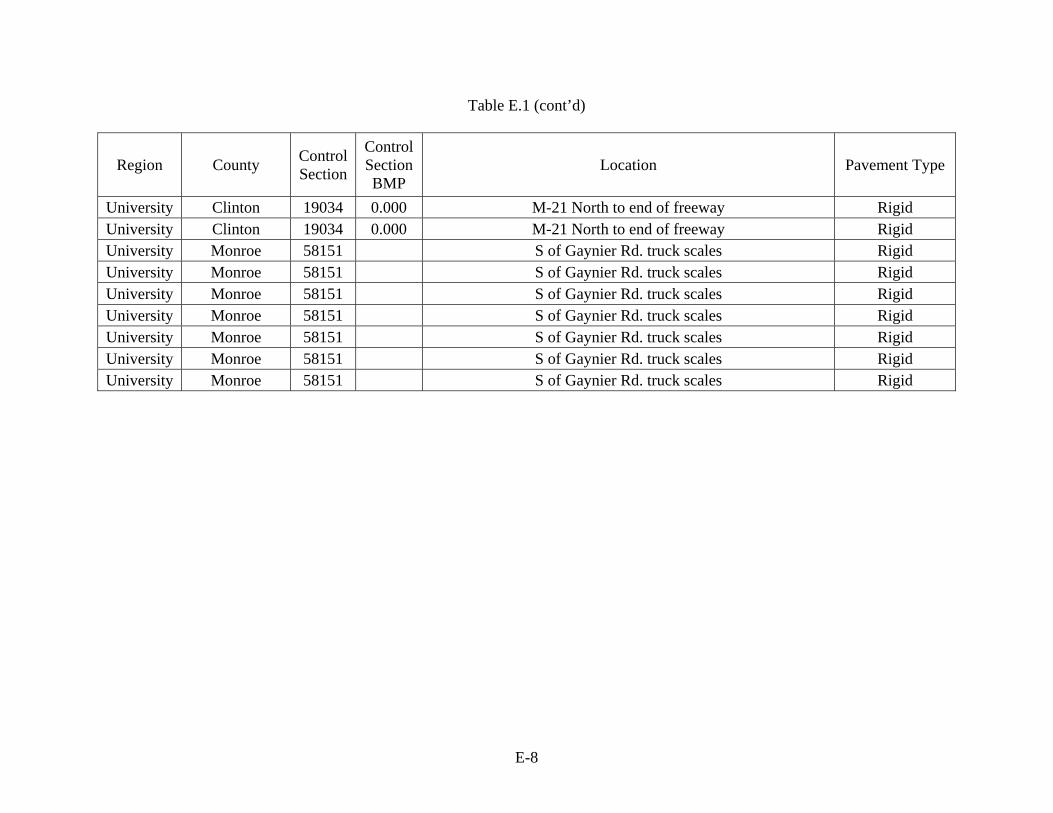
E-8
Table E.1 (cont’d)
Region County Control Section
Control Section BMP
Location Pavement Type
University Clinton 19034 0.000 M-21 North to end of freeway Rigid University Clinton 19034 0.000 M-21 North to end of freeway Rigid University Monroe 58151 S of Gaynier Rd. truck scales Rigid University Monroe 58151 S of Gaynier Rd. truck scales Rigid University Monroe 58151 S of Gaynier Rd. truck scales Rigid University Monroe 58151 S of Gaynier Rd. truck scales Rigid University Monroe 58151 S of Gaynier Rd. truck scales Rigid University Monroe 58151 S of Gaynier Rd. truck scales Rigid University Monroe 58151 S of Gaynier Rd. truck scales Rigid
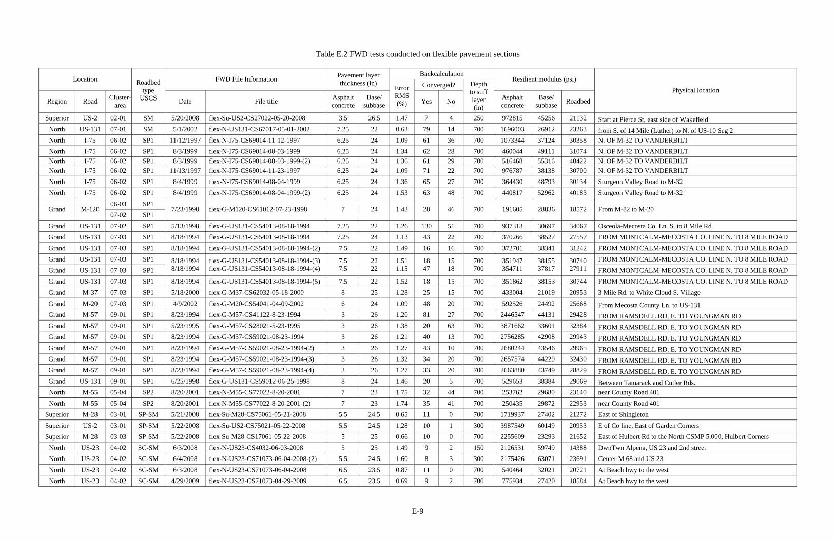
E-9
Table E.2 FWD tests conducted on flexible pavement sections Backcalculation
Location FWD File Information Pavement layer thickness (in) Converged?
Resilient modulus (psi)
Region Road Cluster- area
Roadbed type
USCS Date File title Asphalt concrete
Base/ subbase
Error RMS (%) Yes No
Depth to stiff layer (in)
Asphalt concrete
Base/ subbase Roadbed
Physical location
Superior US-2 02-01 SM 5/20/2008 flex-Su-US2-CS27022-05-20-2008 3.5 26.5 1.47 7 4 250 972815 45256 21132 Start at Pierce St, east side of Wakefield North US-131 07-01 SM 5/1/2002 flex-N-US131-CS67017-05-01-2002 7.25 22 0.63 79 14 700 1696003 26912 23263 from S. of 14 Mile (Luther) to N. of US-10 Seg 2 North I-75 06-02 SP1 11/12/1997 flex-N-I75-CS69014-11-12-1997 6.25 24 1.09 61 36 700 1073344 37124 30358 N. OF M-32 TO VANDERBILT North I-75 06-02 SP1 8/3/1999 flex-N-I75-CS69014-08-03-1999 6.25 24 1.34 62 28 700 460044 49111 31074 N. OF M-32 TO VANDERBILT North I-75 06-02 SP1 8/3/1999 flex-N-I75-CS69014-08-03-1999-(2) 6.25 24 1.36 61 29 700 516468 55316 40422 N. OF M-32 TO VANDERBILT North I-75 06-02 SP1 11/13/1997 flex-N-I75-CS69014-11-23-1997 6.25 24 1.09 71 22 700 976787 38138 30700 N. OF M-32 TO VANDERBILT North I-75 06-02 SP1 8/4/1999 flex-N-I75-CS69014-08-04-1999 6.25 24 1.36 65 27 700 364430 48793 30134 Sturgeon Valley Road to M-32 North I-75 06-02 SP1 8/4/1999 flex-N-I75-CS69014-08-04-1999-(2) 6.25 24 1.53 63 48 700 440817 52962 40183 Sturgeon Valley Road to M-32
06-03 SP1 Grand M-120
07-02 SP1 7/23/1998 flex-G-M120-CS61012-07-23-1998 7 24 1.43 28 46 700 191605 28836 18572 From M-82 to M-20
Grand US-131 07-02 SP1 5/13/1998 flex-G-US131-CS54013-08-18-1994 7.25 22 1.26 130 51 700 937313 30697 34067 Osceola-Mecosta Co. Ln. S. to 8 Mile Rd Grand US-131 07-03 SP1 8/18/1994 flex-G-US131-CS54013-08-18-1994 7.25 24 1.13 43 22 700 370266 38527 27557 FROM MONTCALM-MECOSTA CO. LINE N. TO 8 MILE ROAD Grand US-131 07-03 SP1 8/18/1994 flex-G-US131-CS54013-08-18-1994-(2) 7.5 22 1.49 16 16 700 372701 38341 31242 FROM MONTCALM-MECOSTA CO. LINE N. TO 8 MILE ROAD Grand US-131 07-03 SP1 FROM MONTCALM-MECOSTA CO. LINE N. TO 8 MILE ROAD Grand US-131 07-03 SP1
8/18/1994 8/18/1994
flex-G-US131-CS54013-08-18-1994-(3) flex-G-US131-CS54013-08-18-1994-(4)
7.5 7.5
22 22
1.51 1.15
18 47
15 18
700 700
351947 354711
38155 37817
30740 27911 FROM MONTCALM-MECOSTA CO. LINE N. TO 8 MILE ROAD
Grand US-131 07-03 SP1 8/18/1994 flex-G-US131-CS54013-08-18-1994-(5) 7.5 22 1.52 18 15 700 351862 38153 30744 FROM MONTCALM-MECOSTA CO. LINE N. TO 8 MILE ROAD Grand M-37 07-03 SP1 5/18/2000 flex-G-M37-CS62032-05-18-2000 8 25 1.28 25 15 700 433004 21019 20953 3 Mile Rd. to White Cloud S. Village Grand M-20 07-03 SP1 4/9/2002 flex-G-M20-CS54041-04-09-2002 6 24 1.09 48 20 700 592526 24492 25668 From Mecosta County Ln. to US-131 Grand M-57 09-01 SP1 8/23/1994 flex-G-M57-CS41122-8-23-1994 3 26 1.20 81 27 700 2446547 44131 29428 FROM RAMSDELL RD. E. TO YOUNGMAN RD Grand M-57 09-01 SP1 5/23/1995 flex-G-M57-CS28021-5-23-1995 3 26 1.38 20 63 700 3871662 33601 32384 FROM RAMSDELL RD. E. TO YOUNGMAN RD Grand M-57 09-01 SP1 8/23/1994 flex-G-M57-CS59021-08-23-1994 3 26 1.21 40 13 700 2756285 42908 29943 FROM RAMSDELL RD. E. TO YOUNGMAN RD Grand M-57 09-01 SP1 8/23/1994 flex-G-M57-CS59021-08-23-1994-(2) 3 26 1.27 43 10 700 2680244 43546 29965 FROM RAMSDELL RD. E. TO YOUNGMAN RD Grand M-57 09-01 SP1 8/23/1994 flex-G-M57-CS59021-08-23-1994-(3) 3 26 1.32 34 20 700 2657574 44229 32430 FROM RAMSDELL RD. E. TO YOUNGMAN RD Grand M-57 09-01 SP1 8/23/1994 flex-G-M57-CS59021-08-23-1994-(4) 3 26 1.27 33 20 700 2663880 43749 28829 FROM RAMSDELL RD. E. TO YOUNGMAN RD Grand US-131 09-01 SP1 6/25/1998 flex-G-US131-CS59012-06-25-1998 8 24 1.46 20 5 700 529653 38384 29069 Between Tamarack and Cutler Rds. North M-55 05-04 SP2 8/20/2001 flex-N-M55-CS77022-8-20-2001 7 23 1.75 32 44 700 253762 29680 23140 near County Road 401 North M-55 05-04 SP2 8/20/2001 flex-N-M55-CS77022-8-20-2001-(2) 7 23 1.74 35 41 700 250435 29872 22953 near County Road 401
Superior M-28 03-01 SP-SM 5/21/2008 flex-Su-M28-CS75061-05-21-2008 5.5 24.5 0.65 11 0 700 1719937 27402 21272 East of Shingleton Superior US-2 03-01 SP-SM 5/22/2008 flex-Su-US2-CS75021-05-22-2008 5.5 24.5 1.28 10 1 300 3987549 60149 20953 E of Co line, East of Garden Corners Superior M-28 03-03 SP-SM 5/22/2008 flex-Su-M28-CS17061-05-22-2008 5 25 0.66 10 0 700 2255609 23293 21652 East of Hulbert Rd to the North CSMP 5.000, Hulbert Corners
North US-23 04-02 SC-SM 6/3/2008 flex-N-US23-CS4032-06-03-2008 5 25 1.49 9 2 150 2126531 59749 14388 DwnTwn Alpena, US 23 and 2nd street North US-23 04-02 SC-SM 6/4/2008 flex-N-US23-CS71073-06-04-2008-(2) 5.5 24.5 1.60 8 3 300 2175426 63071 23691 Center M 68 and US 23 North US-23 04-02 SC-SM 6/3/2008 flex-N-US23-CS71073-06-04-2008 6.5 23.5 0.87 11 0 700 540464 32021 20721 At Beach hwy to the west North US-23 04-02 SC-SM 4/29/2009 flex-N-US23-CS71073-04-29-2009 6.5 23.5 0.69 9 2 700 775934 27420 18584 At Beach hwy to the west
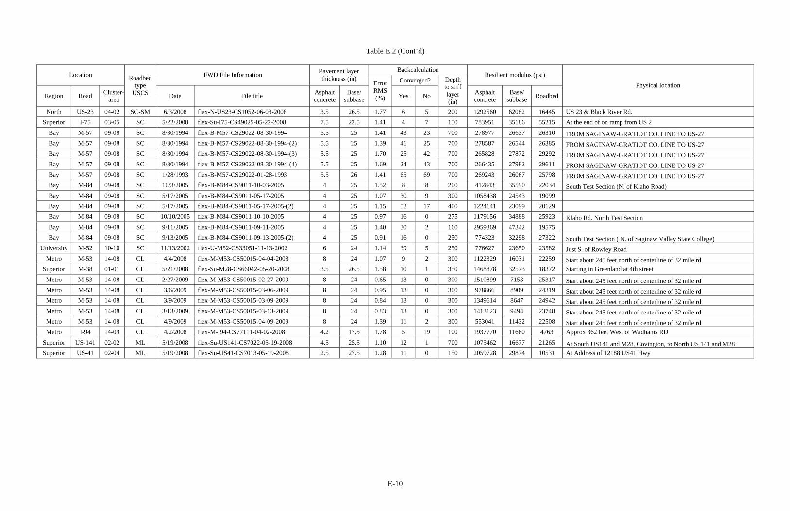
E-10
Table E.2 (Cont’d) Backcalculation
Location FWD File Information Pavement layer thickness (in) Converged?
Resilient modulus (psi)
Region Road Cluster- area
Roadbed type
USCS Date File title Asphalt concrete
Base/ subbase
Error RMS (%) Yes No
Depth to stiff layer (in)
Asphalt concrete
Base/ subbase Roadbed
Physical location
North US-23 04-02 SC-SM 6/3/2008 flex-N-US23-CS1052-06-03-2008 3.5 26.5 1.77 6 5 200 1292560 62082 16445 US 23 & Black River Rd. Superior I-75 03-05 SC 5/22/2008 flex-Su-I75-CS49025-05-22-2008 7.5 22.5 1.41 4 7 150 783951 35186 55215 At the end of on ramp from US 2
Bay M-57 09-08 SC 8/30/1994 flex-B-M57-CS29022-08-30-1994 5.5 25 1.41 43 23 700 278977 26637 26310 FROM SAGINAW-GRATIOT CO. LINE TO US-27 Bay M-57 09-08 SC 8/30/1994 flex-B-M57-CS29022-08-30-1994-(2) 5.5 25 1.39 41 25 700 278587 26544 26385 FROM SAGINAW-GRATIOT CO. LINE TO US-27 Bay M-57 09-08 SC 8/30/1994 flex-B-M57-CS29022-08-30-1994-(3) 5.5 25 1.70 25 42 700 265828 27872 29292 FROM SAGINAW-GRATIOT CO. LINE TO US-27 Bay M-57 09-08 SC 8/30/1994 flex-B-M57-CS29022-08-30-1994-(4) 5.5 25 1.69 24 43 700 266435 27982 29611 FROM SAGINAW-GRATIOT CO. LINE TO US-27 Bay M-57 09-08 SC 1/28/1993 flex-B-M57-CS29022-01-28-1993 5.5 26 1.41 65 69 700 269243 26067 25798 FROM SAGINAW-GRATIOT CO. LINE TO US-27 Bay M-84 09-08 SC 10/3/2005 flex-B-M84-CS9011-10-03-2005 4 25 1.52 8 8 200 412843 35590 22034 South Test Section (N. of Klaho Road) Bay M-84 09-08 SC 5/17/2005 flex-B-M84-CS9011-05-17-2005 4 25 1.07 30 9 300 1058438 24543 19099 Bay M-84 09-08 SC 5/17/2005 flex-B-M84-CS9011-05-17-2005-(2) 4 25 1.15 52 17 400 1224141 23099 20129 Bay M-84 09-08 SC 10/10/2005 flex-B-M84-CS9011-10-10-2005 4 25 0.97 16 0 275 1179156 34888 25923 Klaho Rd. North Test Section Bay M-84 09-08 SC 9/11/2005 flex-B-M84-CS9011-09-11-2005 4 25 1.40 30 2 160 2959369 47342 19575 Bay M-84 09-08 SC 9/13/2005 flex-B-M84-CS9011-09-13-2005-(2) 4 25 0.91 16 0 250 774323 32298 27322 South Test Section ( N. of Saginaw Valley State College)
University M-52 10-10 SC 11/13/2002 flex-U-M52-CS33051-11-13-2002 6 24 1.14 39 5 250 776627 23650 23582 Just S. of Rowley Road Metro M-53 14-08 CL 4/4/2008 flex-M-M53-CS50015-04-04-2008 8 24 1.07 9 2 300 1122329 16031 22259 Start about 245 feet north of centerline of 32 mile rd
Superior M-38 01-01 CL 5/21/2008 flex-Su-M28-CS66042-05-20-2008 3.5 26.5 1.58 10 1 350 1468878 32573 18372 Starting in Greenland at 4th street Metro M-53 14-08 CL 2/27/2009 flex-M-M53-CS50015-02-27-2009 8 24 0.65 13 0 300 1510899 7153 25317 Start about 245 feet north of centerline of 32 mile rd Metro M-53 14-08 CL 3/6/2009 flex-M-M53-CS50015-03-06-2009 8 24 0.95 13 0 300 978866 8909 24319 Start about 245 feet north of centerline of 32 mile rd Metro M-53 14-08 CL 3/9/2009 flex-M-M53-CS50015-03-09-2009 8 24 0.84 13 0 300 1349614 8647 24942 Start about 245 feet north of centerline of 32 mile rd Metro M-53 14-08 CL 3/13/2009 flex-M-M53-CS50015-03-13-2009 8 24 0.83 13 0 300 1413123 9494 23748 Start about 245 feet north of centerline of 32 mile rd Metro M-53 14-08 CL 4/9/2009 flex-M-M53-CS50015-04-09-2009 8 24 1.39 11 2 300 553041 11432 22508 Start about 245 feet north of centerline of 32 mile rd Metro I-94 14-09 CL 4/2/2008 flex-M-I94-CS77111-04-02-2008 4.2 17.5 1.78 5 19 100 1937770 11660 4763 Approx 362 feet West of Wadhams RD
Superior US-141 02-02 ML 5/19/2008 flex-Su-US141-CS7022-05-19-2008 4.5 25.5 1.10 12 1 700 1075462 16677 21265 At South US141 and M28, Covington, to North US 141 and M28 Superior US-41 02-04 ML 5/19/2008 flex-Su-US41-CS7013-05-19-2008 2.5 27.5 1.28 11 0 150 2059728 29874 10531 At Address of 12188 US41 Hwy
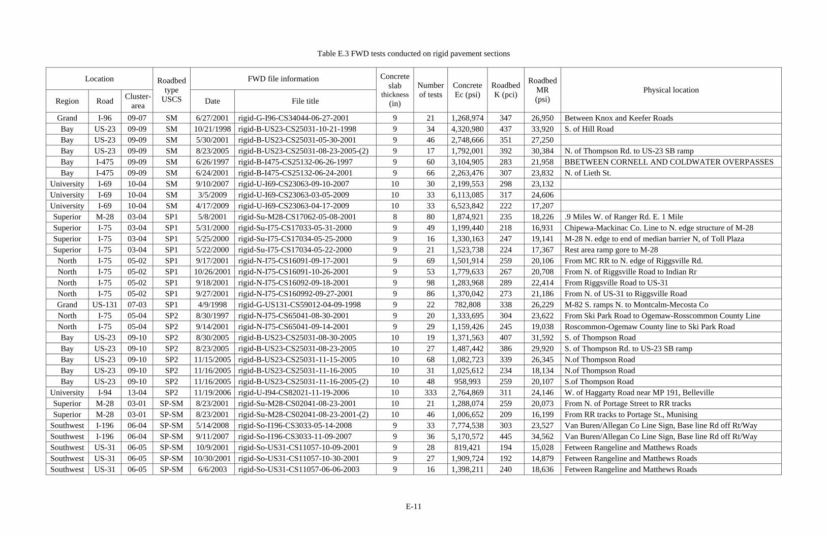
E-11
Table E.3 FWD tests conducted on rigid pavement sections
Location FWD file information
Region Road Cluster- area
Roadbed type
USCS Date File title
Concrete slab
thickness (in)
Number of tests
Concrete Ec (psi)
Roadbed K (pci)
Roadbed MR (psi)
Physical location
Grand I-96 09-07 SM 6/27/2001 rigid-G-I96-CS34044-06-27-2001 9 21 1,268,974 347 26,950 Between Knox and Keefer Roads Bay US-23 09-09 SM 10/21/1998 rigid-B-US23-CS25031-10-21-1998 9 34 4,320,980 437 33,920 S. of Hill Road Bay US-23 09-09 SM 5/30/2001 rigid-B-US23-CS25031-05-30-2001 9 46 2,748,666 351 27,250 Bay US-23 09-09 SM 8/23/2005 rigid-B-US23-CS25031-08-23-2005-(2) 9 17 1,792,001 392 30,384 N. of Thompson Rd. to US-23 SB ramp Bay I-475 09-09 SM 6/26/1997 rigid-B-I475-CS25132-06-26-1997 9 60 3,104,905 283 21,958 BBETWEEN CORNELL AND COLDWATER OVERPASSES Bay I-475 09-09 SM 6/24/2001 rigid-B-I475-CS25132-06-24-2001 9 66 2,263,476 307 23,832 N. of Lieth St.
University I-69 10-04 SM 9/10/2007 rigid-U-I69-CS23063-09-10-2007 10 30 2,199,553 298 23,132 University I-69 10-04 SM 3/5/2009 rigid-U-I69-CS23063-03-05-2009 10 33 6,113,085 317 24,606 University I-69 10-04 SM 4/17/2009 rigid-U-I69-CS23063-04-17-2009 10 33 6,523,842 222 17,207 Superior M-28 03-04 SP1 5/8/2001 rigid-Su-M28-CS17062-05-08-2001 8 80 1,874,921 235 18,226 .9 Miles W. of Ranger Rd. E. 1 Mile Superior I-75 03-04 SP1 5/31/2000 rigid-Su-I75-CS17033-05-31-2000 9 49 1,199,440 218 16,931 Chipewa-Mackinac Co. Line to N. edge structure of M-28 Superior I-75 03-04 SP1 5/25/2000 rigid-Su-I75-CS17034-05-25-2000 9 16 1,330,163 247 19,141 M-28 N. edge to end of median barrier N, of Toll Plaza Superior I-75 03-04 SP1 5/22/2000 rigid-Su-I75-CS17034-05-22-2000 9 21 1,523,738 224 17,367 Rest area ramp gore to M-28
North I-75 05-02 SP1 9/17/2001 rigid-N-I75-CS16091-09-17-2001 9 69 1,501,914 259 20,106 From MC RR to N. edge of Riggsville Rd. North I-75 05-02 SP1 10/26/2001 rigid-N-I75-CS16091-10-26-2001 9 53 1,779,633 267 20,708 From N. of Riggsville Road to Indian Rr North I-75 05-02 SP1 9/18/2001 rigid-N-I75-CS16092-09-18-2001 9 98 1,283,968 289 22,414 From Riggsville Road to US-31 North I-75 05-02 SP1 9/27/2001 rigid-N-I75-CS160992-09-27-2001 9 86 1,370,042 273 21,186 From N. of US-31 to Riggsville Road Grand US-131 07-03 SP1 4/9/1998 rigid-G-US131-CS59012-04-09-1998 9 22 782,808 338 26,229 M-82 S. ramps N. to Montcalm-Mecosta Co North I-75 05-04 SP2 8/30/1997 rigid-N-I75-CS65041-08-30-2001 9 20 1,333,695 304 23,622 From Ski Park Road to Ogemaw-Rosscommon County Line North I-75 05-04 SP2 9/14/2001 rigid-N-I75-CS65041-09-14-2001 9 29 1,159,426 245 19,038 Roscommon-Ogemaw County line to Ski Park Road Bay US-23 09-10 SP2 8/30/2005 rigid-B-US23-CS25031-08-30-2005 10 19 1,371,563 407 31,592 S. of Thompson Road Bay US-23 09-10 SP2 8/23/2005 rigid-B-US23-CS25031-08-23-2005 10 27 1,487,442 386 29,920 S. of Thompson Rd. to US-23 SB ramp Bay US-23 09-10 SP2 11/15/2005 rigid-B-US23-CS25031-11-15-2005 10 68 1,082,723 339 26,345 N.of Thompson Road Bay US-23 09-10 SP2 11/16/2005 rigid-B-US23-CS25031-11-16-2005 10 31 1,025,612 234 18,134 N.of Thompson Road Bay US-23 09-10 SP2 11/16/2005 rigid-B-US23-CS25031-11-16-2005-(2) 10 48 958,993 259 20,107 S.of Thompson Road
University I-94 13-04 SP2 11/19/2006 rigid-U-I94-CS82021-11-19-2006 10 333 2,764,869 311 24,146 W. of Haggarty Road near MP 191, Belleville Superior M-28 03-01 SP-SM 8/23/2001 rigid-Su-M28-CS02041-08-23-2001 10 21 1,288,074 259 20,073 From N. of Portage Street to RR tracks Superior M-28 03-01 SP-SM 8/23/2001 rigid-Su-M28-CS02041-08-23-2001-(2) 10 46 1,006,652 209 16,199 From RR tracks to Portage St., Munising
Southwest I-196 06-04 SP-SM 5/14/2008 rigid-So-I196-CS3033-05-14-2008 9 33 7,774,538 303 23,527 Van Buren/Allegan Co Line Sign, Base line Rd off Rt/Way Southwest I-196 06-04 SP-SM 9/11/2007 rigid-So-I196-CS3033-11-09-2007 9 36 5,170,572 445 34,562 Van Buren/Allegan Co Line Sign, Base line Rd off Rt/Way Southwest US-31 06-05 SP-SM 10/9/2001 rigid-So-US31-CS11057-10-09-2001 9 28 819,421 194 15,028 Fetween Rangeline and Matthews Roads Southwest US-31 06-05 SP-SM 10/30/2001 rigid-So-US31-CS11057-10-30-2001 9 27 1,909,724 192 14,879 Fetween Rangeline and Matthews Roads Southwest US-31 06-05 SP-SM 6/6/2003 rigid-So-US31-CS11057-06-06-2003 9 16 1,398,211 240 18,636 Fetween Rangeline and Matthews Roads
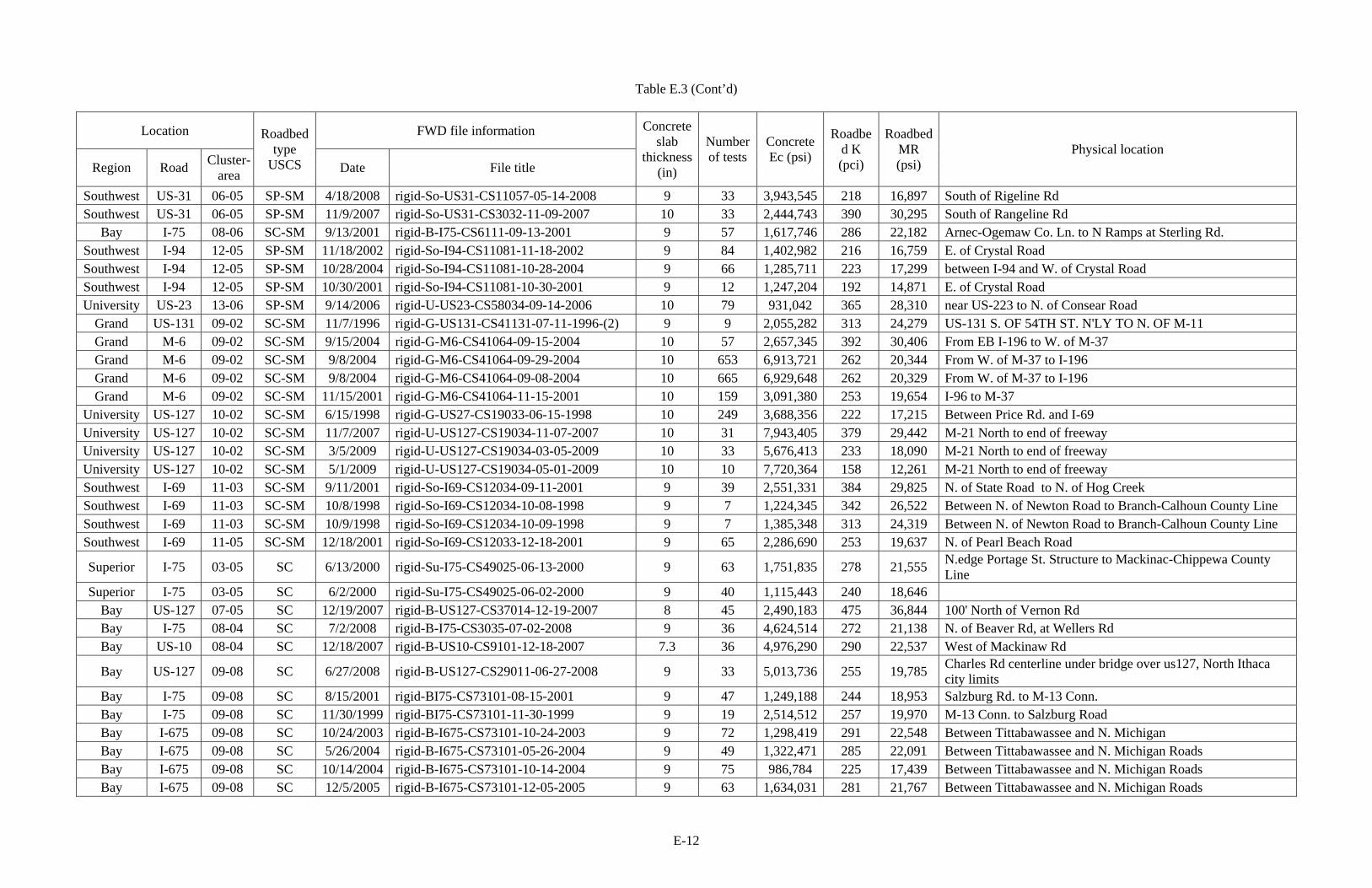
E-12
Table E.3 (Cont’d)
Location FWD file information
Region Road Cluster- area
Roadbed type
USCS Date File title
Concrete slab
thickness (in)
Number of tests
Concrete Ec (psi)
Roadbed K (pci)
Roadbed MR (psi)
Physical location
Southwest US-31 06-05 SP-SM 4/18/2008 rigid-So-US31-CS11057-05-14-2008 9 33 3,943,545 218 16,897 South of Rigeline Rd Southwest US-31 06-05 SP-SM 11/9/2007 rigid-So-US31-CS3032-11-09-2007 10 33 2,444,743 390 30,295 South of Rangeline Rd
Bay I-75 08-06 SC-SM 9/13/2001 rigid-B-I75-CS6111-09-13-2001 9 57 1,617,746 286 22,182 Arnec-Ogemaw Co. Ln. to N Ramps at Sterling Rd. Southwest I-94 12-05 SP-SM 11/18/2002 rigid-So-I94-CS11081-11-18-2002 9 84 1,402,982 216 16,759 E. of Crystal Road Southwest I-94 12-05 SP-SM 10/28/2004 rigid-So-I94-CS11081-10-28-2004 9 66 1,285,711 223 17,299 between I-94 and W. of Crystal Road Southwest I-94 12-05 SP-SM 10/30/2001 rigid-So-I94-CS11081-10-30-2001 9 12 1,247,204 192 14,871 E. of Crystal Road University US-23 13-06 SP-SM 9/14/2006 rigid-U-US23-CS58034-09-14-2006 10 79 931,042 365 28,310 near US-223 to N. of Consear Road
Grand US-131 09-02 SC-SM 11/7/1996 rigid-G-US131-CS41131-07-11-1996-(2) 9 9 2,055,282 313 24,279 US-131 S. OF 54TH ST. N'LY TO N. OF M-11 Grand M-6 09-02 SC-SM 9/15/2004 rigid-G-M6-CS41064-09-15-2004 10 57 2,657,345 392 30,406 From EB I-196 to W. of M-37 Grand M-6 09-02 SC-SM 9/8/2004 rigid-G-M6-CS41064-09-29-2004 10 653 6,913,721 262 20,344 From W. of M-37 to I-196 Grand M-6 09-02 SC-SM 9/8/2004 rigid-G-M6-CS41064-09-08-2004 10 665 6,929,648 262 20,329 From W. of M-37 to I-196 Grand M-6 09-02 SC-SM 11/15/2001 rigid-G-M6-CS41064-11-15-2001 10 159 3,091,380 253 19,654 I-96 to M-37
University US-127 10-02 SC-SM 6/15/1998 rigid-G-US27-CS19033-06-15-1998 10 249 3,688,356 222 17,215 Between Price Rd. and I-69 University US-127 10-02 SC-SM 11/7/2007 rigid-U-US127-CS19034-11-07-2007 10 31 7,943,405 379 29,442 M-21 North to end of freeway University US-127 10-02 SC-SM 3/5/2009 rigid-U-US127-CS19034-03-05-2009 10 33 5,676,413 233 18,090 M-21 North to end of freeway University US-127 10-02 SC-SM 5/1/2009 rigid-U-US127-CS19034-05-01-2009 10 10 7,720,364 158 12,261 M-21 North to end of freeway Southwest I-69 11-03 SC-SM 9/11/2001 rigid-So-I69-CS12034-09-11-2001 9 39 2,551,331 384 29,825 N. of State Road to N. of Hog Creek Southwest I-69 11-03 SC-SM 10/8/1998 rigid-So-I69-CS12034-10-08-1998 9 7 1,224,345 342 26,522 Between N. of Newton Road to Branch-Calhoun County Line Southwest I-69 11-03 SC-SM 10/9/1998 rigid-So-I69-CS12034-10-09-1998 9 7 1,385,348 313 24,319 Between N. of Newton Road to Branch-Calhoun County Line Southwest I-69 11-05 SC-SM 12/18/2001 rigid-So-I69-CS12033-12-18-2001 9 65 2,286,690 253 19,637 N. of Pearl Beach Road
Superior I-75 03-05 SC 6/13/2000 rigid-Su-I75-CS49025-06-13-2000 9 63 1,751,835 278 21,555 N.edge Portage St. Structure to Mackinac-Chippewa County Line
Superior I-75 03-05 SC 6/2/2000 rigid-Su-I75-CS49025-06-02-2000 9 40 1,115,443 240 18,646 Bay US-127 07-05 SC 12/19/2007 rigid-B-US127-CS37014-12-19-2007 8 45 2,490,183 475 36,844 100' North of Vernon Rd Bay I-75 08-04 SC 7/2/2008 rigid-B-I75-CS3035-07-02-2008 9 36 4,624,514 272 21,138 N. of Beaver Rd, at Wellers Rd Bay US-10 08-04 SC 12/18/2007 rigid-B-US10-CS9101-12-18-2007 7.3 36 4,976,290 290 22,537 West of Mackinaw Rd
Bay US-127 09-08 SC 6/27/2008 rigid-B-US127-CS29011-06-27-2008 9 33 5,013,736 255 19,785 Charles Rd centerline under bridge over us127, North Ithaca city limits
Bay I-75 09-08 SC 8/15/2001 rigid-BI75-CS73101-08-15-2001 9 47 1,249,188 244 18,953 Salzburg Rd. to M-13 Conn. Bay I-75 09-08 SC 11/30/1999 rigid-BI75-CS73101-11-30-1999 9 19 2,514,512 257 19,970 M-13 Conn. to Salzburg Road Bay I-675 09-08 SC 10/24/2003 rigid-B-I675-CS73101-10-24-2003 9 72 1,298,419 291 22,548 Between Tittabawassee and N. Michigan Bay I-675 09-08 SC 5/26/2004 rigid-B-I675-CS73101-05-26-2004 9 49 1,322,471 285 22,091 Between Tittabawassee and N. Michigan Roads Bay I-675 09-08 SC 10/14/2004 rigid-B-I675-CS73101-10-14-2004 9 75 986,784 225 17,439 Between Tittabawassee and N. Michigan Roads Bay I-675 09-08 SC 12/5/2005 rigid-B-I675-CS73101-12-05-2005 9 63 1,634,031 281 21,767 Between Tittabawassee and N. Michigan Roads
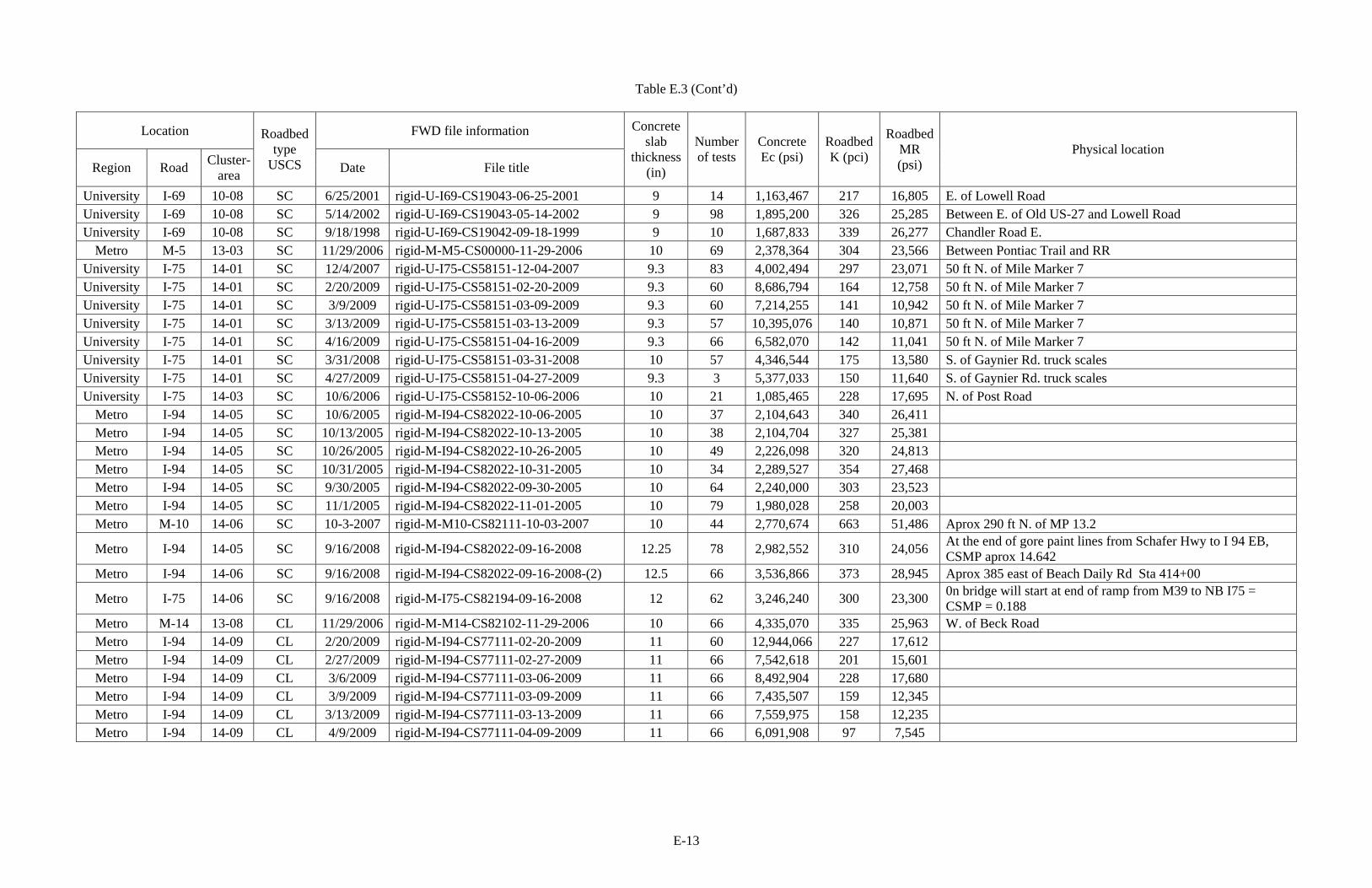
E-13
Table E.3 (Cont’d)
Location FWD file information
Region Road Cluster- area
Roadbed type
USCS Date File title
Concrete slab
thickness (in)
Number of tests
Concrete Ec (psi)
Roadbed K (pci)
Roadbed MR (psi)
Physical location
University I-69 10-08 SC 6/25/2001 rigid-U-I69-CS19043-06-25-2001 9 14 1,163,467 217 16,805 E. of Lowell Road University I-69 10-08 SC 5/14/2002 rigid-U-I69-CS19043-05-14-2002 9 98 1,895,200 326 25,285 Between E. of Old US-27 and Lowell Road University I-69 10-08 SC 9/18/1998 rigid-U-I69-CS19042-09-18-1999 9 10 1,687,833 339 26,277 Chandler Road E.
Metro M-5 13-03 SC 11/29/2006 rigid-M-M5-CS00000-11-29-2006 10 69 2,378,364 304 23,566 Between Pontiac Trail and RR University I-75 14-01 SC 12/4/2007 rigid-U-I75-CS58151-12-04-2007 9.3 83 4,002,494 297 23,071 50 ft N. of Mile Marker 7 University I-75 14-01 SC 2/20/2009 rigid-U-I75-CS58151-02-20-2009 9.3 60 8,686,794 164 12,758 50 ft N. of Mile Marker 7 University I-75 14-01 SC 3/9/2009 rigid-U-I75-CS58151-03-09-2009 9.3 60 7,214,255 141 10,942 50 ft N. of Mile Marker 7 University I-75 14-01 SC 3/13/2009 rigid-U-I75-CS58151-03-13-2009 9.3 57 10,395,076 140 10,871 50 ft N. of Mile Marker 7 University I-75 14-01 SC 4/16/2009 rigid-U-I75-CS58151-04-16-2009 9.3 66 6,582,070 142 11,041 50 ft N. of Mile Marker 7 University I-75 14-01 SC 3/31/2008 rigid-U-I75-CS58151-03-31-2008 10 57 4,346,544 175 13,580 S. of Gaynier Rd. truck scales University I-75 14-01 SC 4/27/2009 rigid-U-I75-CS58151-04-27-2009 9.3 3 5,377,033 150 11,640 S. of Gaynier Rd. truck scales University I-75 14-03 SC 10/6/2006 rigid-U-I75-CS58152-10-06-2006 10 21 1,085,465 228 17,695 N. of Post Road
Metro I-94 14-05 SC 10/6/2005 rigid-M-I94-CS82022-10-06-2005 10 37 2,104,643 340 26,411 Metro I-94 14-05 SC 10/13/2005 rigid-M-I94-CS82022-10-13-2005 10 38 2,104,704 327 25,381 Metro I-94 14-05 SC 10/26/2005 rigid-M-I94-CS82022-10-26-2005 10 49 2,226,098 320 24,813 Metro I-94 14-05 SC 10/31/2005 rigid-M-I94-CS82022-10-31-2005 10 34 2,289,527 354 27,468 Metro I-94 14-05 SC 9/30/2005 rigid-M-I94-CS82022-09-30-2005 10 64 2,240,000 303 23,523 Metro I-94 14-05 SC 11/1/2005 rigid-M-I94-CS82022-11-01-2005 10 79 1,980,028 258 20,003 Metro M-10 14-06 SC 10-3-2007 rigid-M-M10-CS82111-10-03-2007 10 44 2,770,674 663 51,486 Aprox 290 ft N. of MP 13.2
Metro I-94 14-05 SC 9/16/2008 rigid-M-I94-CS82022-09-16-2008 12.25 78 2,982,552 310 24,056 At the end of gore paint lines from Schafer Hwy to I 94 EB, CSMP aprox 14.642
Metro I-94 14-06 SC 9/16/2008 rigid-M-I94-CS82022-09-16-2008-(2) 12.5 66 3,536,866 373 28,945 Aprox 385 east of Beach Daily Rd Sta 414+00
Metro I-75 14-06 SC 9/16/2008 rigid-M-I75-CS82194-09-16-2008 12 62 3,246,240 300 23,300 0n bridge will start at end of ramp from M39 to NB I75 = CSMP = 0.188
Metro M-14 13-08 CL 11/29/2006 rigid-M-M14-CS82102-11-29-2006 10 66 4,335,070 335 25,963 W. of Beck Road Metro I-94 14-09 CL 2/20/2009 rigid-M-I94-CS77111-02-20-2009 11 60 12,944,066 227 17,612 Metro I-94 14-09 CL 2/27/2009 rigid-M-I94-CS77111-02-27-2009 11 66 7,542,618 201 15,601 Metro I-94 14-09 CL 3/6/2009 rigid-M-I94-CS77111-03-06-2009 11 66 8,492,904 228 17,680 Metro I-94 14-09 CL 3/9/2009 rigid-M-I94-CS77111-03-09-2009 11 66 7,435,507 159 12,345 Metro I-94 14-09 CL 3/13/2009 rigid-M-I94-CS77111-03-13-2009 11 66 7,559,975 158 12,235 Metro I-94 14-09 CL 4/9/2009 rigid-M-I94-CS77111-04-09-2009 11 66 6,091,908 97 7,545
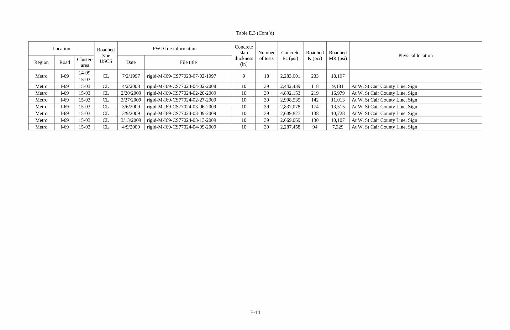
E-14
Table E.3 (Cont’d)
Location FWD file information
Region Road Cluster- area
Roadbed type
USCS Date File title
Concrete slab
thickness (in)
Number of tests
Concrete Ec (psi)
Roadbed K (pci)
Roadbed MR (psi) Physical location
14-09 Metro I-69 15-03
CL 7/2/1997 rigid-M-I69-CS77023-07-02-1997 9 18 2,283,001 233 18,107
Metro I-69 15-03 CL 4/2/2008 rigid-M-I69-CS77024-04-02-2008 10 39 2,442,439 118 9,181 At W. St Cair County Line, Sign Metro I-69 15-03 CL 2/20/2009 rigid-M-I69-CS77024-02-20-2009 10 39 4,892,153 219 16,979 At W. St Cair County Line, Sign Metro I-69 15-03 CL 2/27/2009 rigid-M-I69-CS77024-02-27-2009 10 39 2,908,535 142 11,013 At W. St Cair County Line, Sign Metro I-69 15-03 CL 3/6/2009 rigid-M-I69-CS77024-03-06-2009 10 39 2,837,078 174 13,515 At W. St Cair County Line, Sign Metro I-69 15-03 CL 3/9/2009 rigid-M-I69-CS77024-03-09-2009 10 39 2,609,827 138 10,728 At W. St Cair County Line, Sign Metro I-69 15-03 CL 3/13/2009 rigid-M-I69-CS77024-03-13-2009 10 39 2,669,069 130 10,107 At W. St Cair County Line, Sign Metro I-69 15-03 CL 4/9/2009 rigid-M-I69-CS77024-04-09-2009 10 39 2,287,458 94 7,329 At W. St Cair County Line, Sign

E-15
The deflection basin data and the backcalculated pavement layer moduli for each of the FWD tests conducted on flexible and rigid pavement structures are listed in Tables E.4 and E.5, respectively.