ECE544: Communication Networks-II, Spring 2010 D. Raychaudhuri Lecture 4 Includes teaching materials...
69
ECE544: Communication Networks-II, Spring 2010 D. Raychaudhuri Lecture 4 Includes teaching materials from L. Peterson
-
date post
20-Dec-2015 -
Category
Documents
-
view
216 -
download
1
Transcript of ECE544: Communication Networks-II, Spring 2010 D. Raychaudhuri Lecture 4 Includes teaching materials...
ECE544: Communication Networks-II, Spring 2010
D. Raychaudhuri
Lecture 4
Includes teaching materials from L. Peterson
Today’s Lecture
• IP basics• Routing principles
– distance vector (RIP)– link state (OSPF)
IP Basics
Best Effort Service ModelGlobal Addressing SchemeARP & DHCP
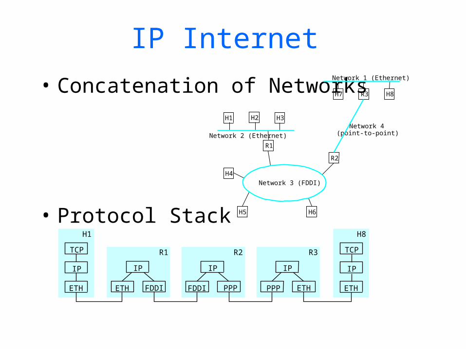
IP Internet
• Concatenation of Networks
• Protocol Stack
R2
R1
H4
H5
H3H2H1
Network 2 (Ethernet)
Network 1 (Ethernet)
H6
Network 3 (FDDI)
Network 4(point-to-point)
H7 R3 H8
R1
ETH FDDI
IPIP
ETH
TCP R2
FDDI PPP
IP
R3
PPP ETH
IP
H1
IP
ETH
TCP
H8
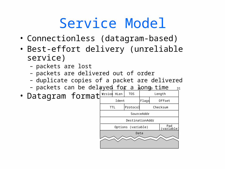
Service Model• Connectionless (datagram-based)• Best-effort delivery (unreliable service)
– packets are lost– packets are delivered out of order– duplicate copies of a packet are delivered– packets can be delayed for a long time
• Datagram format Version HLen TOS Length
Ident Flags Offset
TTL Protocol Checksum
SourceAddr
DestinationAddr
Options (variable) Pad(variable)
0 4 8 16 19 31
Data
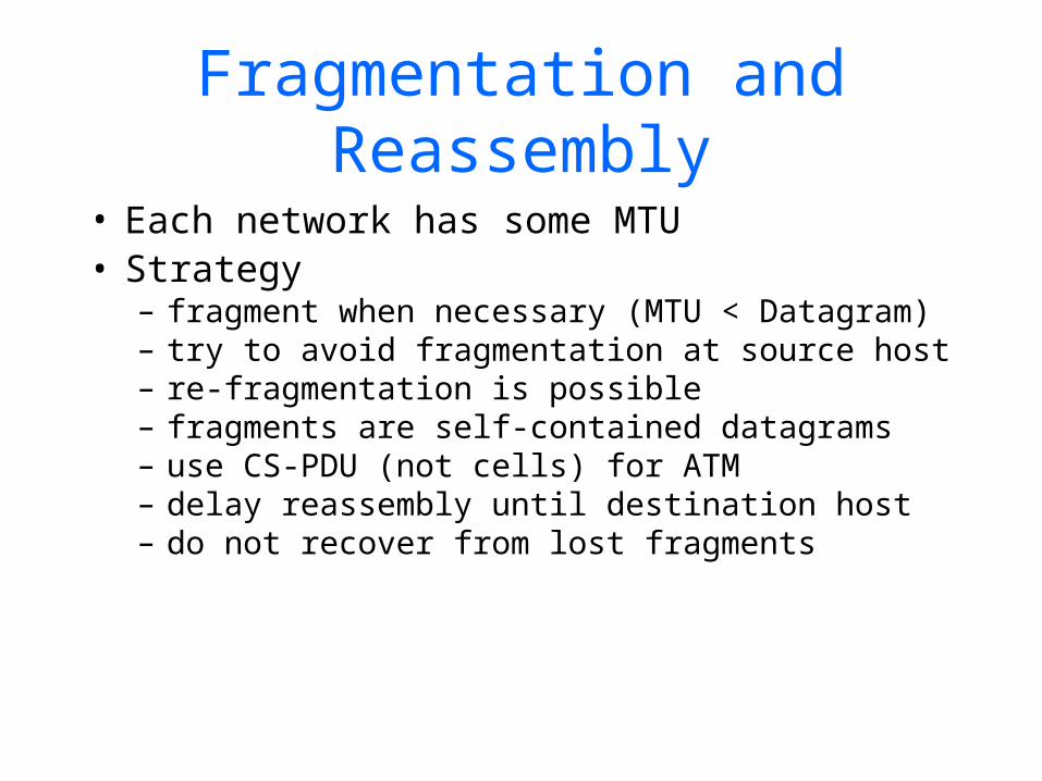
Fragmentation and Reassembly
• Each network has some MTU• Strategy
– fragment when necessary (MTU < Datagram)– try to avoid fragmentation at source host– re-fragmentation is possible – fragments are self-contained datagrams– use CS-PDU (not cells) for ATM– delay reassembly until destination host– do not recover from lost fragments
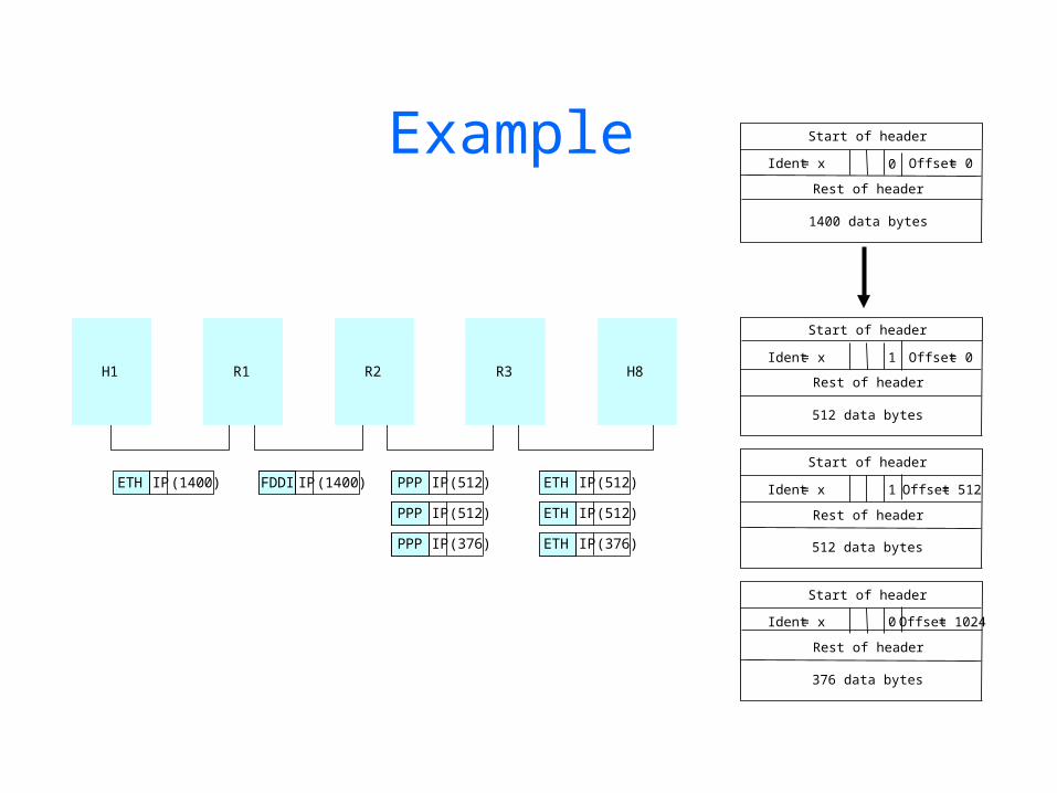
Example
H1 R1 R2 R3 H8
ETH IP (1400) FDDI IP (1400) PPP IP (512)
PPP IP (376)
PPP IP (512)
ETH IP (512)
ETH IP (376)
ETH IP (512)
Ident = x Offset = 0
Start of header
0
Rest of header
1400 data bytes
Ident = x Offset = 0
Start of header
1
Rest of header
512 data bytes
Ident = x Offset = 512
Start of header
1
Rest of header
512 data bytes
Ident = x Offset = 1024
Start of header
0
Rest of header
376 data bytes
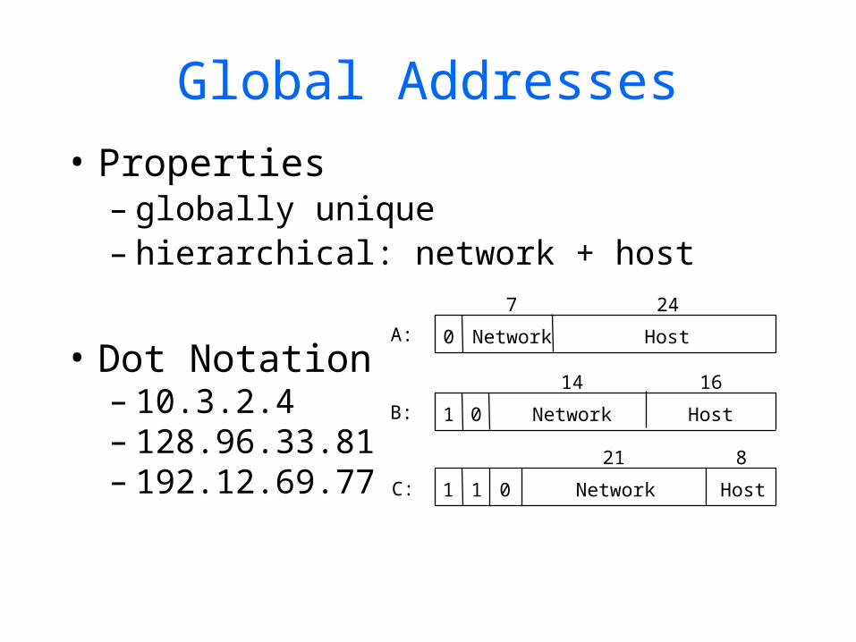
Global Addresses• Properties
– globally unique– hierarchical: network + host
• Dot Notation– 10.3.2.4– 128.96.33.81– 192.12.69.77
Network Host
7 24
0A:
Network Host
14 16
1 0B:
Network Host
21 8
1 1 0C:

Datagram Forwarding • Strategy
– every datagram contains destination’s address– if directly connected to destination network, then forward to
host– if not directly connected to destination network, then
forward to some router– forwarding table maps network number into next hop– each host has a default router– each router maintains a forwarding table
• Example (R2) Network Number Next Hop
1 R3 2 R1 3 interface 1 4 interface 0
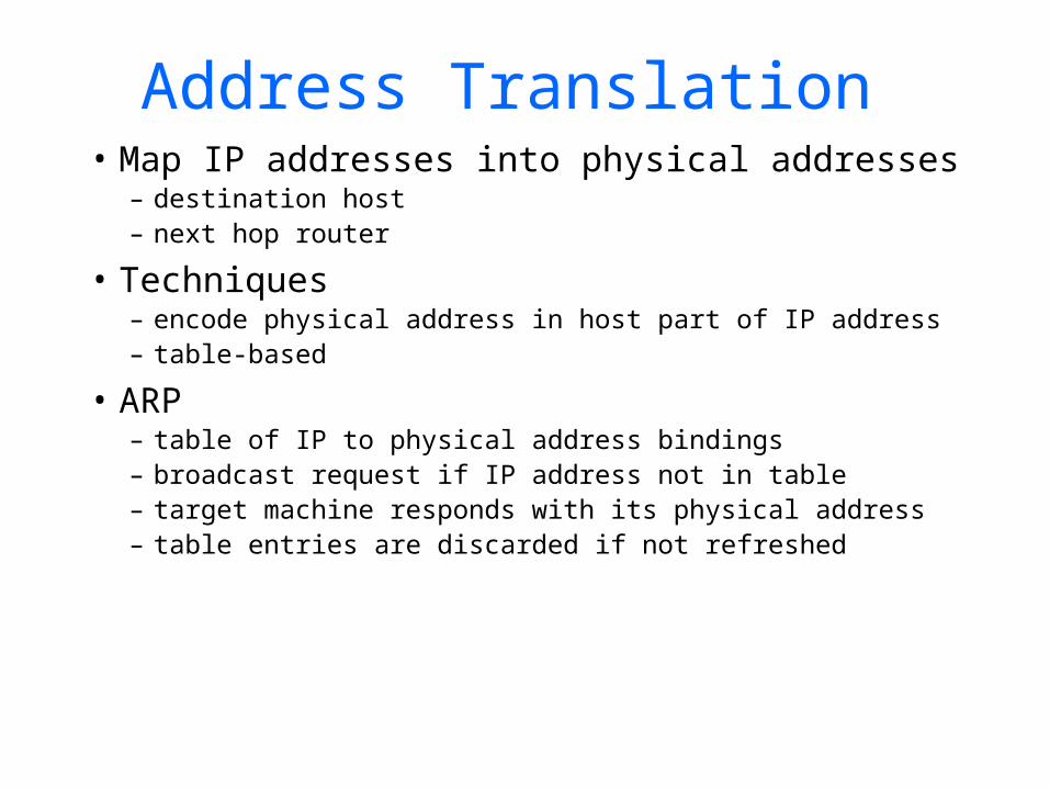
Address Translation • Map IP addresses into physical addresses
– destination host– next hop router
• Techniques– encode physical address in host part of IP address– table-based
• ARP– table of IP to physical address bindings– broadcast request if IP address not in table– target machine responds with its physical address– table entries are discarded if not refreshed
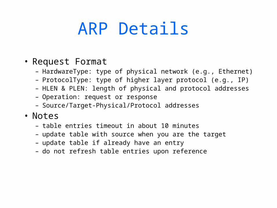
ARP Details
• Request Format– HardwareType: type of physical network (e.g., Ethernet)– ProtocolType: type of higher layer protocol (e.g., IP)– HLEN & PLEN: length of physical and protocol addresses– Operation: request or response – Source/Target-Physical/Protocol addresses
• Notes– table entries timeout in about 10 minutes– update table with source when you are the target – update table if already have an entry– do not refresh table entries upon reference
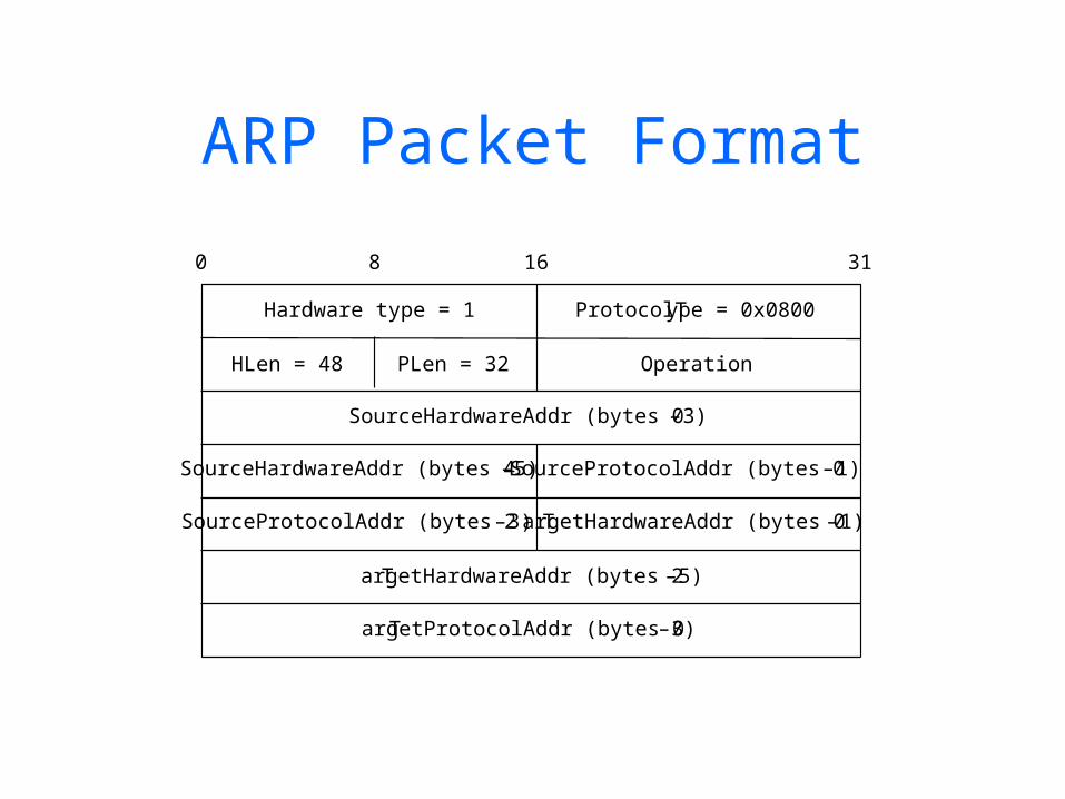
ARP Packet Format
TargetHardwareAddr (bytes 2 – 5)
TargetProtocolAddr (bytes 0 – 3)
SourceProtocolAddr (bytes 2 – 3)
Hardware type = 1 ProtocolType = 0x0800
SourceHardwareAddr (bytes 4 – 5)
TargetHardwareAddr (bytes 0 – 1)
SourceProtocolAddr (bytes 0 – 1)
HLen = 48 PLen = 32 Operation
SourceHardwareAddr (bytes 0 – 3)
0 8 16 31
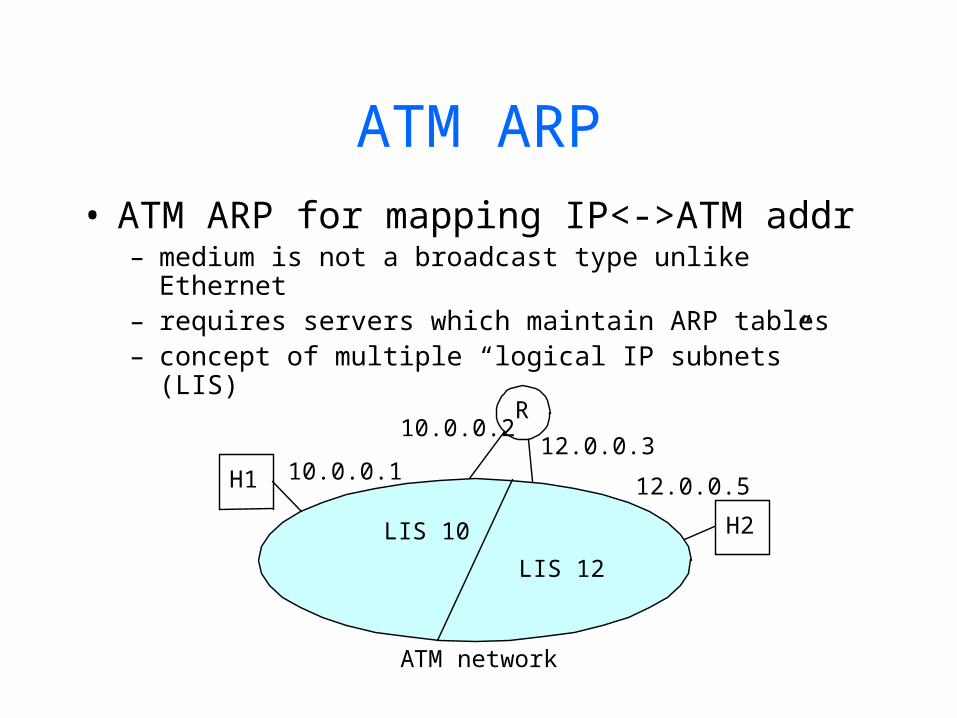
ATM ARP
H2
R
H1
LIS 10
LIS 12
ATM network
10.0.0.2
10.0.0.112.0.0.3
12.0.0.5
• ATM ARP for mapping IP<->ATM addr– medium is not a broadcast type unlike Ethernet– requires servers which maintain ARP tables– concept of multiple “logical IP subnets” (LIS)
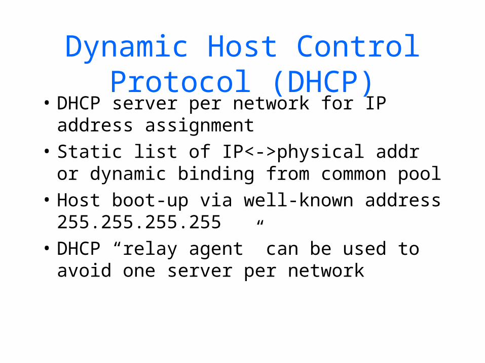
Dynamic Host Control Protocol (DHCP)
• DHCP server per network for IP address assignment
• Static list of IP<->physical addr or dynamic binding from common pool
• Host boot-up via well-known address 255.255.255.255
• DHCP “relay agent” can be used to avoid one server per network

Dynamic Host Control Protocol (DHCP)
• DHCP packet format (runs over UDP)
Operation HType HLen Hops
Xid
Secs Flag
ciaddr
yiaddr
siaddr
giaddr
chaddr (16B)
....
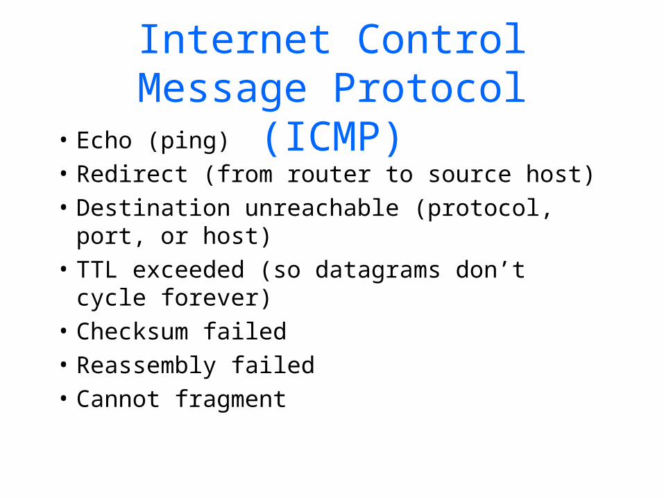
Internet Control Message Protocol (ICMP)
• Echo (ping)• Redirect (from router to source host)• Destination unreachable (protocol, port, or
host)• TTL exceeded (so datagrams don’t cycle
forever)• Checksum failed • Reassembly failed• Cannot fragment
Routing Basics
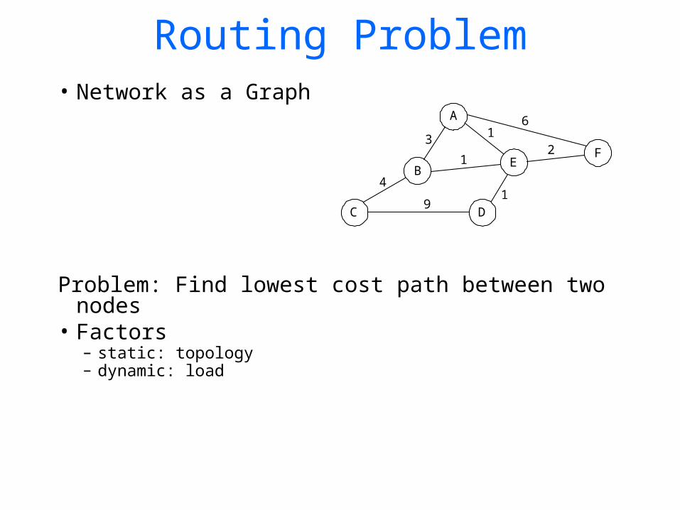
Routing Problem• Network as a Graph
Problem: Find lowest cost path between two nodes
• Factors– static: topology– dynamic: load
4
3
6
21
9
1
1D
A
FE
B
C

Two main approaches• DV: Distance-vector protocols• LS: Link state protocols• Variations of above methods applied
to:– Intra-domain routing (small/med networks)
• RIP, OSPF
– Inter-domain routing (large/global networks)• BGP-4
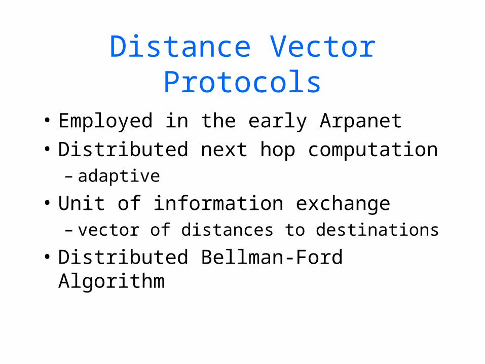
Distance Vector Protocols
• Employed in the early Arpanet• Distributed next hop computation
– adaptive
• Unit of information exchange – vector of distances to destinations
• Distributed Bellman-Ford Algorithm
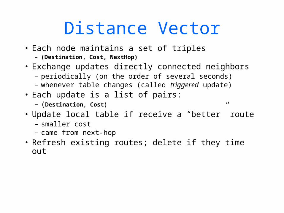
Distance Vector• Each node maintains a set of triples
– (Destination, Cost, NextHop)
• Exchange updates directly connected neighbors– periodically (on the order of several seconds)– whenever table changes (called triggered update)
• Each update is a list of pairs:– (Destination, Cost)
• Update local table if receive a “better” route– smaller cost– came from next-hop
• Refresh existing routes; delete if they time out
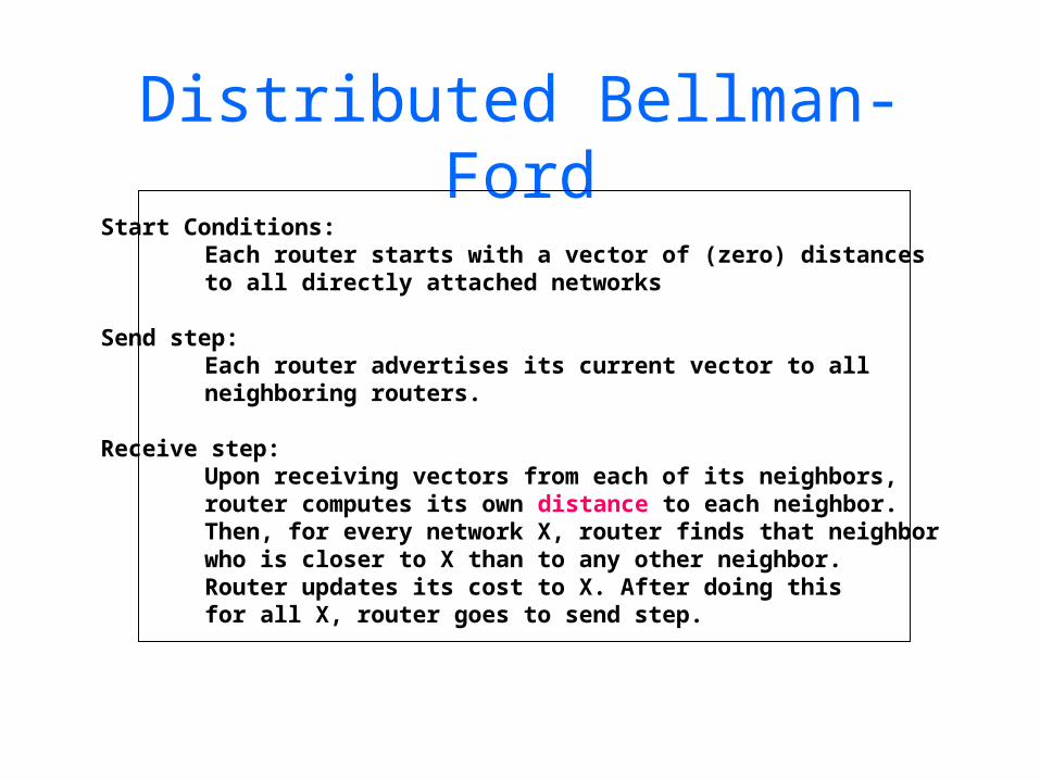
Distributed Bellman-FordStart Conditions:
Each router starts with a vector of (zero) distancesto all directly attached networks
Send step:Each router advertises its current vector to allneighboring routers.
Receive step:Upon receiving vectors from each of its neighbors,router computes its own distance to each neighbor.Then, for every network X, router finds that neighborwho is closer to X than to any other neighbor.Router updates its cost to X. After doing thisfor all X, router goes to send step.
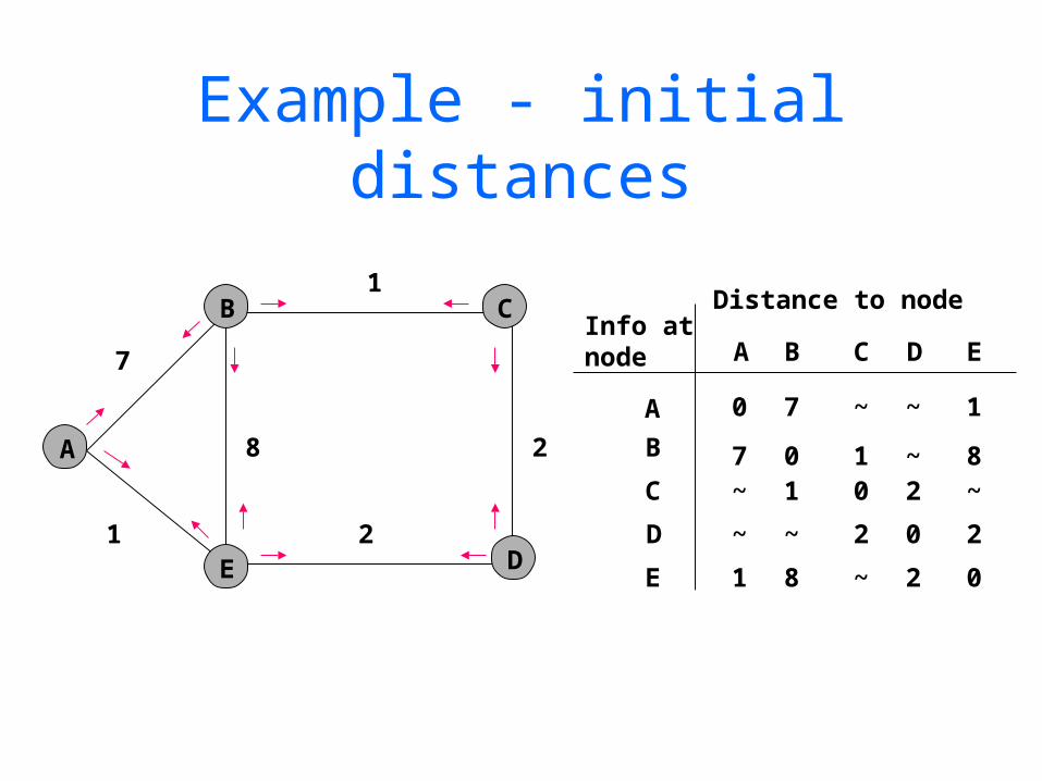
Example - initial distances
A
B
E
C
D
Info atnode
A
B
C
D
A B C
0 7 ~
7 0 1~ 1 0
~ ~ 2
7
1
1
2
28
Distance to node
D
~
~2
0
E 1 8 ~ 2
1
8~
2
0
E
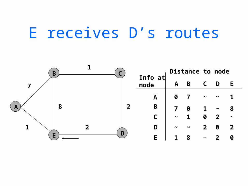
E receives D’s routes
A
B
E
C
D
Info atnode
A
B
C
D
A B C
0 7 ~
7 0 1~ 1 0
~ ~ 2
7
1
1
2
28
Distance to node
D
~
~2
0
E 1 8 ~ 2
1
8~
2
0
E

E updates cost to C
A
B
E
C
D
Info atnode
A
B
C
D
A B C
0 7 ~
7 0 1~ 1 0
~ ~ 2
7
1
1
2
28
Distance to node
D
~
~2
0
E 1 8 4 2
1
8~
2
0
E
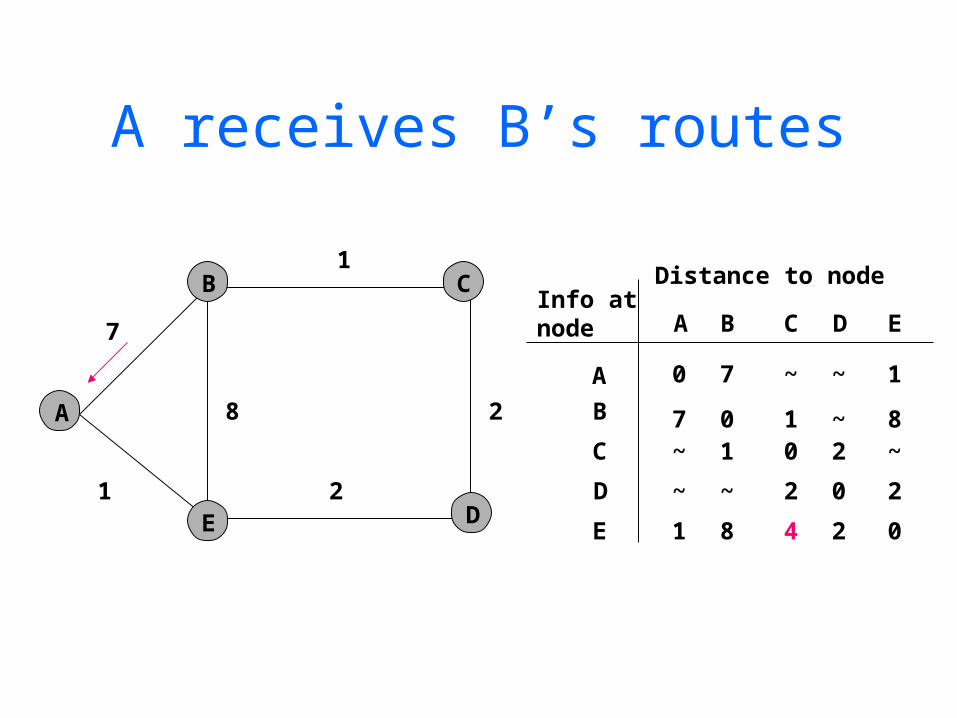
A receives B’s routes
A
B
E
C
D
Info atnode
A
B
C
D
A B C
0 7 ~
7 0 1~ 1 0
~ ~ 2
7
1
1
2
28
Distance to node
D
~
~2
0
E 1 8 4 2
1
8~
2
0
E
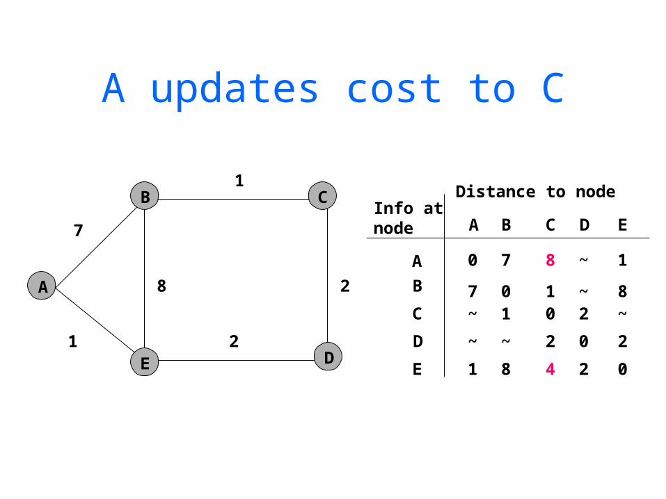
A updates cost to C
A
B
E
C
D
Info atnode
A
B
C
D
A B C
0 7 8
7 0 1~ 1 0
~ ~ 2
7
1
1
2
28
Distance to node
D
~
~2
0
E 1 8 4 2
1
8~
2
0
E
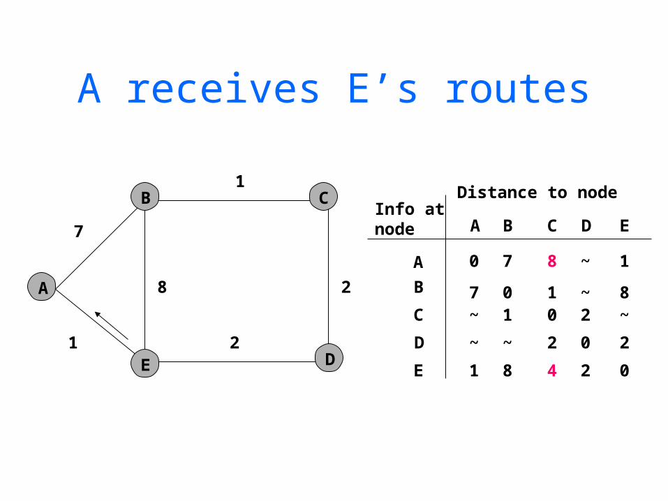
A receives E’s routes
A
B
E
C
D
Info atnode
A
B
C
D
A B C
0 7 8
7 0 1~ 1 0
~ ~ 2
7
1
1
2
28
Distance to node
D
~
~2
0
E 1 8 4 2
1
8~
2
0
E
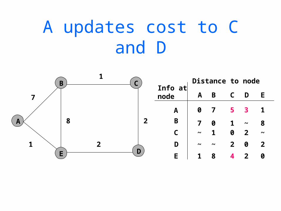
A updates cost to C and D
A
B
E
C
D
Info atnode
A
B
C
D
A B C
0 7 5
7 0 1~ 1 0
~ ~ 2
7
1
1
2
28
Distance to node
D
3
~2
0
E 1 8 4 2
1
8~
2
0
E
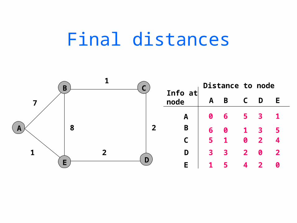
Final distances
A
B C
D
Info atnode
A
B
C
D
A B C
0 6 5
6 0 15 1 0
3 3 2
7
1
1
2
28
Distance to node
D
3
32
0
E 1 5 4 2
1
54
2
0
E
E

Final distances after link failure
A
B C
D
Info atnode
A
B
C
D
A B C
0 7 8
7 0 1
8 1 0
10 3 2
7
1
1
2
28
Distance to node
D
10
3
2
0
E 1 8 9 11
1
8
9
11
0
E
E

View from a node
A
B
E
C
D
dest
A
B
C
D
A B D
1 14 5
7 8 56 9 4
4 11 2
7
1
1
2
28
Next hop
E’s routing table
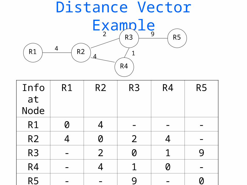
Distance Vector Example
R1 R2
R4
R3 R5
4
2 9
4 1
Info at
Node
R1 R2 R3 R4 R5
R1 0 4 - - -
R2 4 0 2 4 -
R3 - 2 0 1 9
R4 - 4 1 0 -
R5 - - 9 - 0
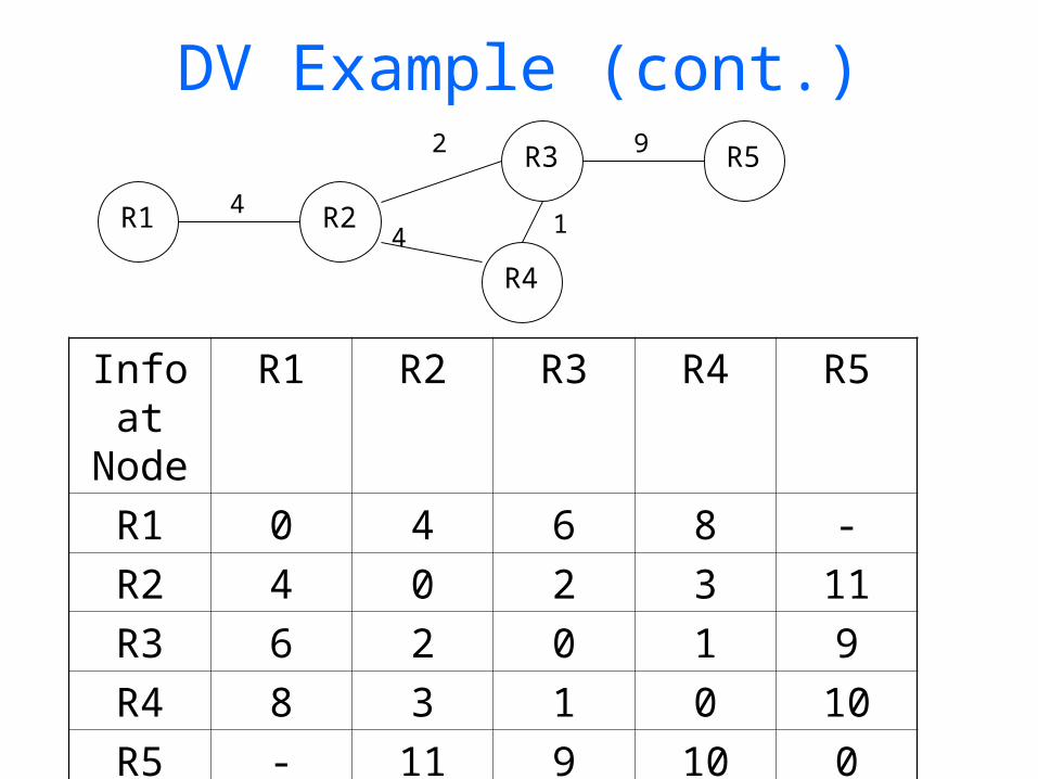
DV Example (cont.)
R1 R2
R4
R3 R5
4
2 9
4 1
Info at
Node
R1 R2 R3 R4 R5
R1 0 4 6 8 -
R2 4 0 2 3 11
R3 6 2 0 1 9
R4 8 3 1 0 10
R5 - 11 9 10 0
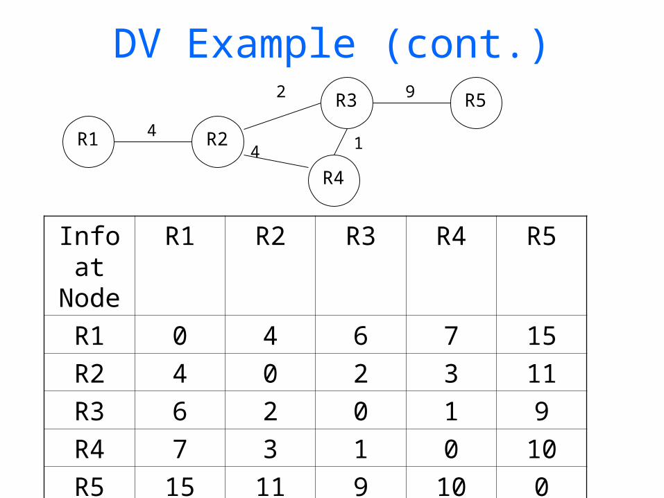
DV Example (cont.)
R1 R2
R4
R3 R5
4
2 9
4 1
Info at
Node
R1 R2 R3 R4 R5
R1 0 4 6 7 15
R2 4 0 2 3 11
R3 6 2 0 1 9
R4 7 3 1 0 10
R5 15 11 9 10 0
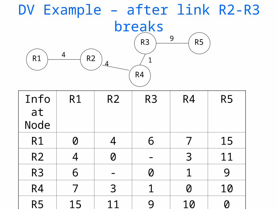
DV Example – after link R2-R3 breaks
R1 R2
R4
R3 R5
4
9
4 1
Info at
Node
R1 R2 R3 R4 R5
R1 0 4 6 7 15
R2 4 0 - 3 11
R3 6 - 0 1 9
R4 7 3 1 0 10
R5 15 11 9 10 0
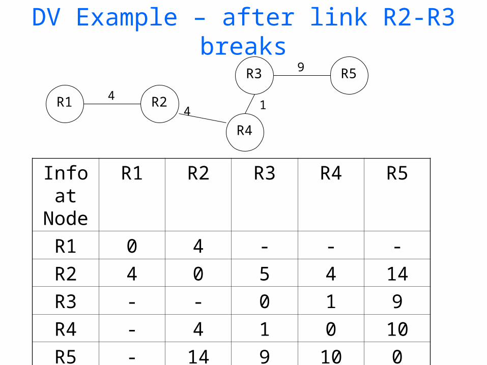
DV Example – after link R2-R3 breaks
R1 R2
R4
R3 R5
4
9
4 1
Info at
Node
R1 R2 R3 R4 R5
R1 0 4 - - -
R2 4 0 5 4 14
R3 - - 0 1 9
R4 - 4 1 0 10
R5 - 14 9 10 0

DV Example – after link R2-R3 breaks
R1 R2
R4
R3 R5
4
9
4 1
Info at
Node
R1 R2 R3 R4 R5
R1 0 4 9 8 18
R2 4 0 5 4 14
R3 9 5 0 1 9
R4 8 4 1 0 10
R5 18 14 9 10 0
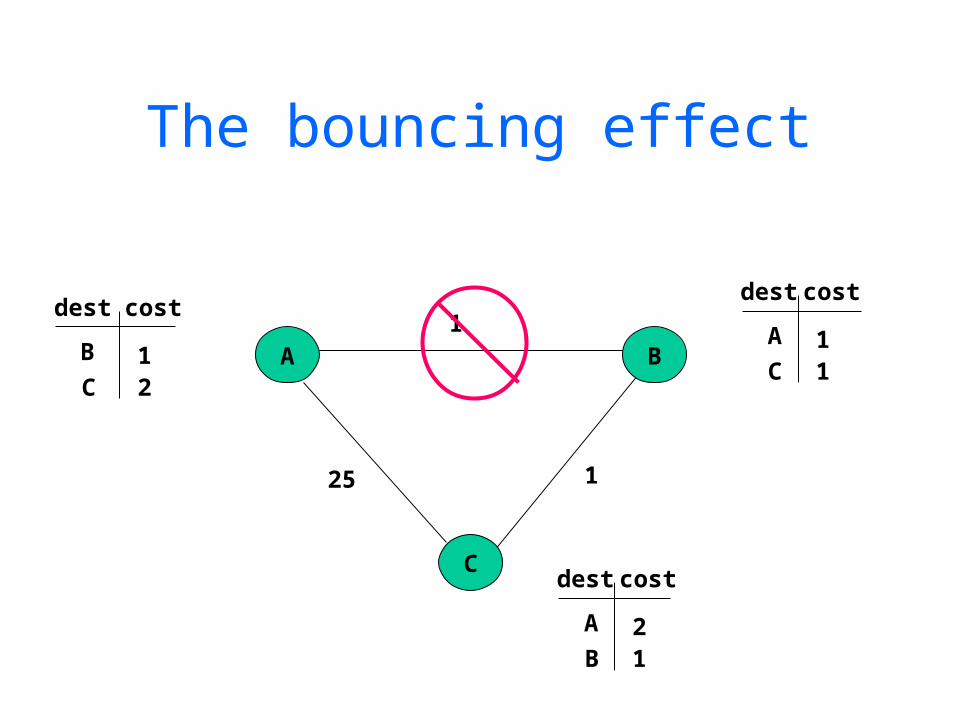
The bouncing effect
A
25
1
1
B
C
B
C 21
dest costA
C 11
dest cost
A
B 12
dest cost
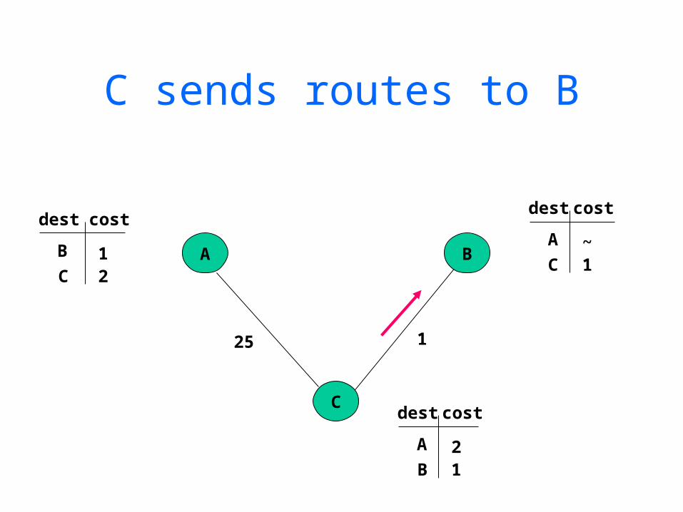
C sends routes to B
A
25 1
B
C
B
C 21
dest costA
C 1~
dest cost
A
B 12
dest cost
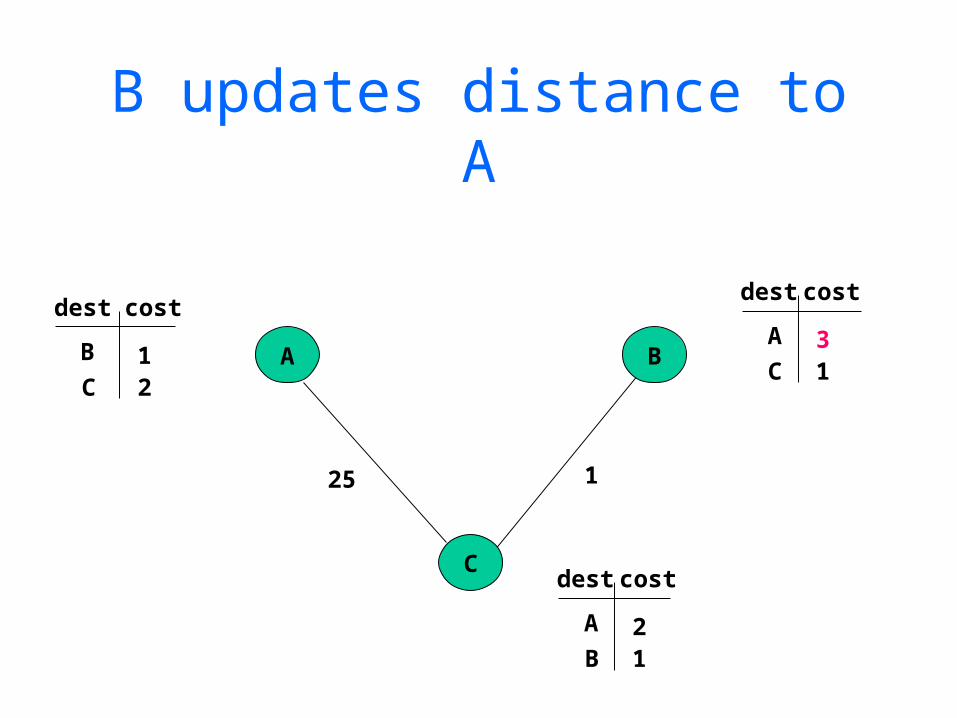
B updates distance to A
A
25 1
B
C
B
C 21
dest costA
C 13
dest cost
A
B 12
dest cost
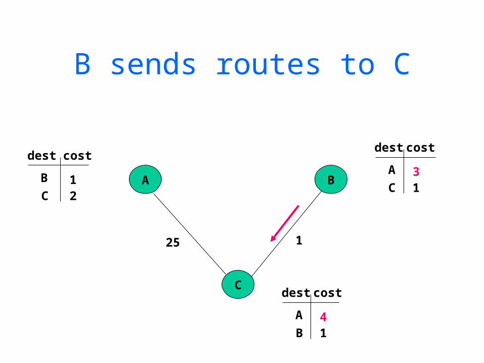
B sends routes to C
A
25 1
B
C
B
C 21
dest costA
C 13
dest cost
A
B 14
dest cost
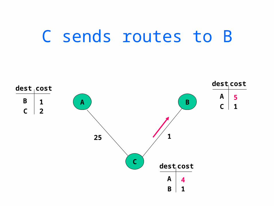
C sends routes to B
A
25 1
B
C
B
C 21
dest costA
C 15
dest cost
A
B 14
dest cost

How are these loops caused?
• Observation 1:– B’s metric increases
• Observation 2:– C picks B as next hop to A– But, the implicit path from C to A
includes itself!
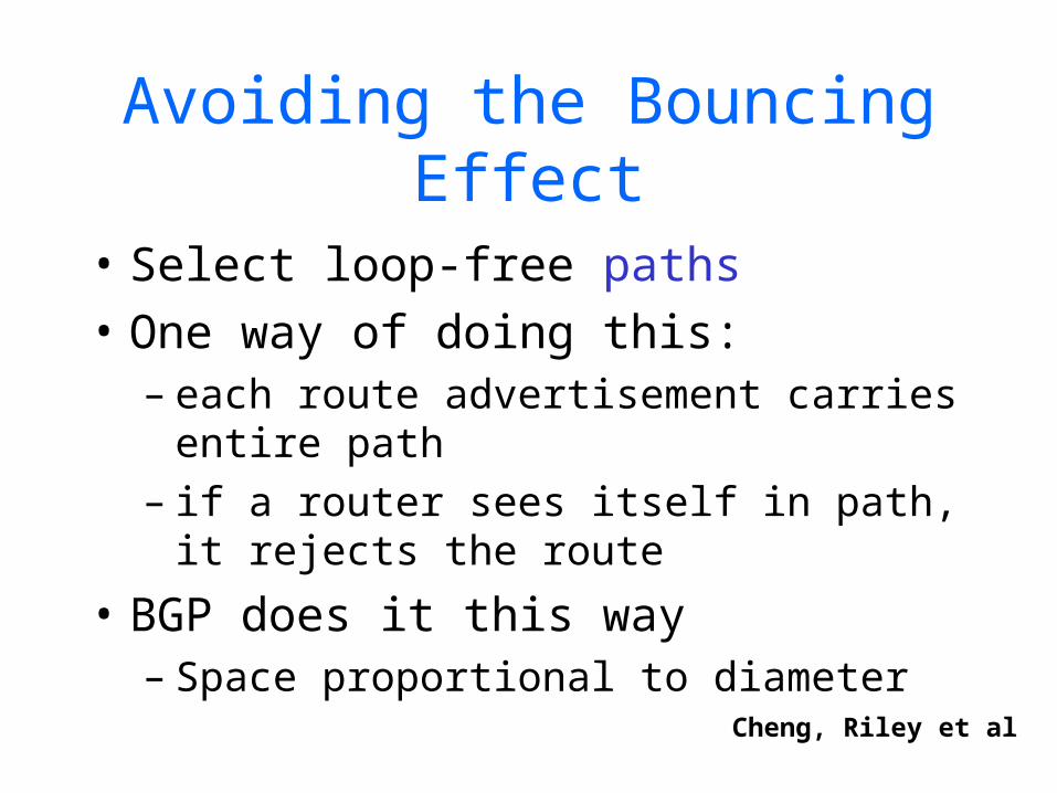
Avoiding the Bouncing Effect
• Select loop-free paths• One way of doing this:
– each route advertisement carries entire path
– if a router sees itself in path, it rejects the route
• BGP does it this way– Space proportional to diameter
Cheng, Riley et al
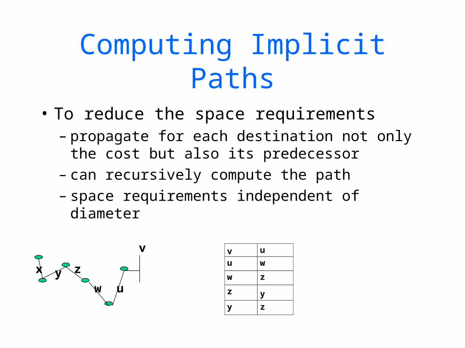
Computing Implicit Paths
• To reduce the space requirements– propagate for each destination not only the
cost but also its predecessor– can recursively compute the path– space requirements independent of diameter
x y z
w u
v v u
u w
w z
z y
y z
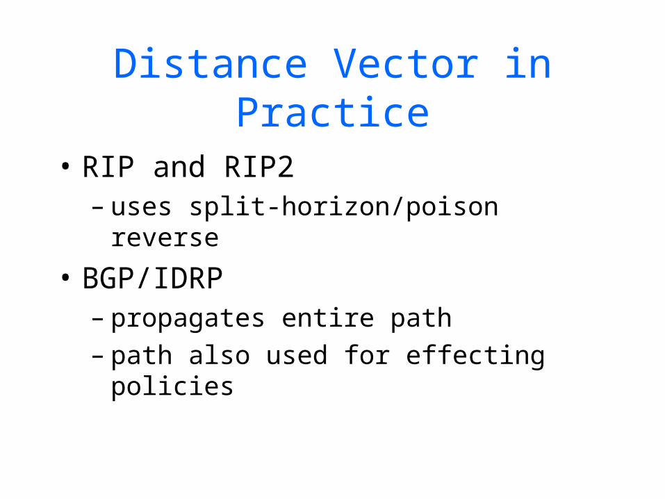
Distance Vector in Practice
• RIP and RIP2– uses split-horizon/poison reverse
• BGP/IDRP– propagates entire path– path also used for effecting policies
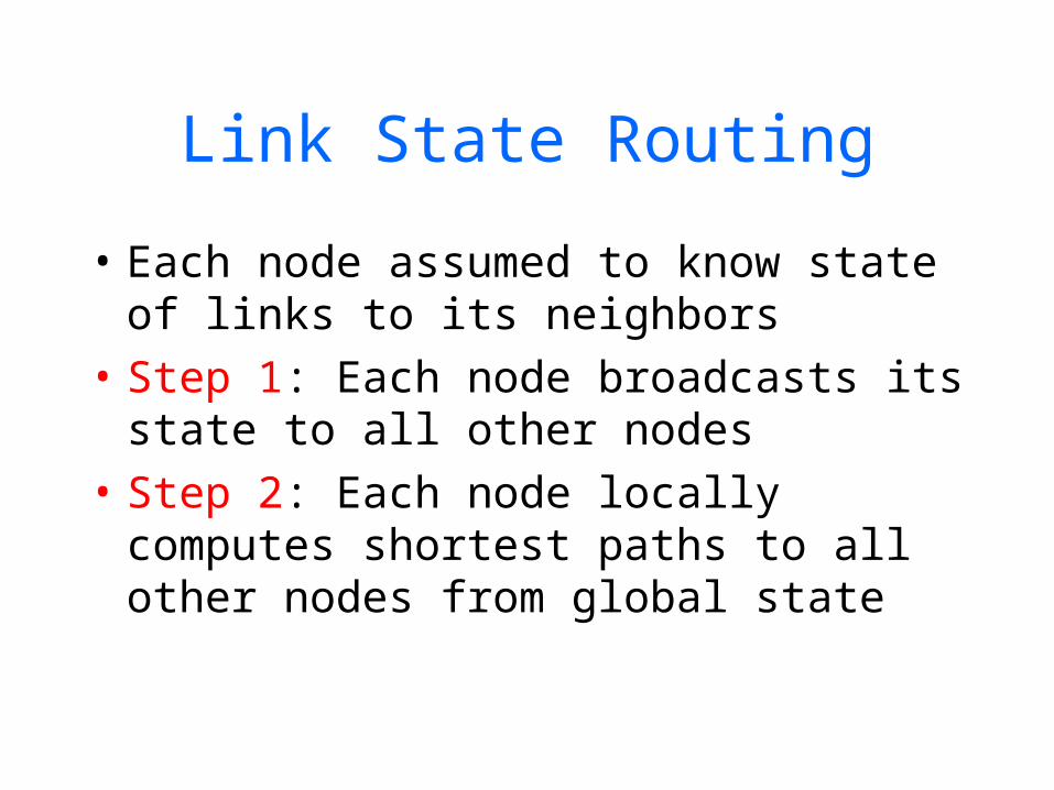
Link State Routing
• Each node assumed to know state of links to its neighbors
• Step 1: Each node broadcasts its state to all other nodes
• Step 2: Each node locally computes shortest paths to all other nodes from global state
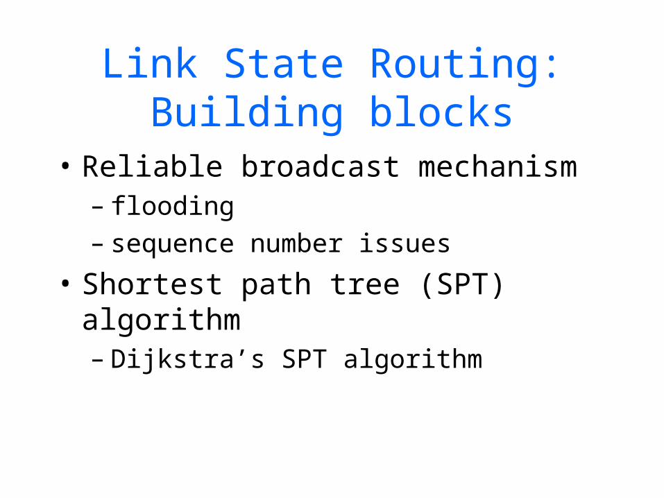
Link State Routing: Building blocks
• Reliable broadcast mechanism– flooding– sequence number issues
• Shortest path tree (SPT) algorithm– Dijkstra’s SPT algorithm
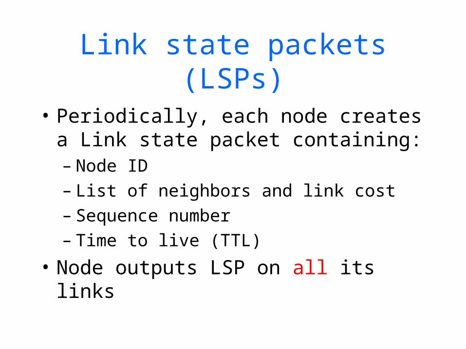
Link state packets (LSPs)
• Periodically, each node creates a Link state packet containing:– Node ID– List of neighbors and link cost– Sequence number– Time to live (TTL)
• Node outputs LSP on all its links
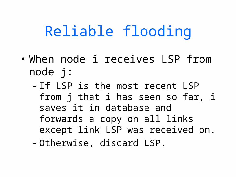
Reliable flooding
• When node i receives LSP from node j:– If LSP is the most recent LSP from j
that i has seen so far, i saves it in database and forwards a copy on all links except link LSP was received on.
– Otherwise, discard LSP.
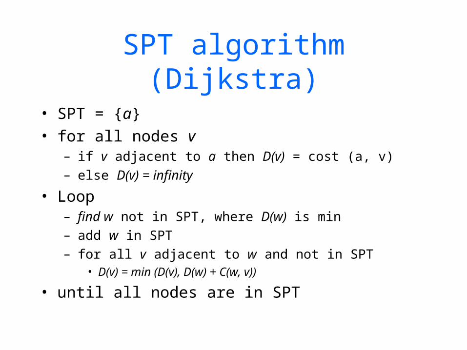
SPT algorithm (Dijkstra)
• SPT = {a}• for all nodes v
– if v adjacent to a then D(v) = cost (a, v)– else D(v) = infinity
• Loop– find w not in SPT, where D(w) is min– add w in SPT– for all v adjacent to w and not in SPT
• D(v) = min (D(v), D(w) + C(w, v))
• until all nodes are in SPT
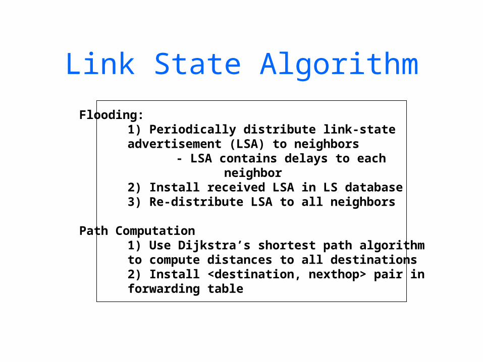
Link State Algorithm
Flooding:1) Periodically distribute link-state advertisement (LSA) to neighbors
- LSA contains delays to eachneighbor
2) Install received LSA in LS database3) Re-distribute LSA to all neighbors
Path Computation1) Use Dijkstra’s shortest path algorithmto compute distances to all destinations2) Install <destination, nexthop> pair inforwarding table
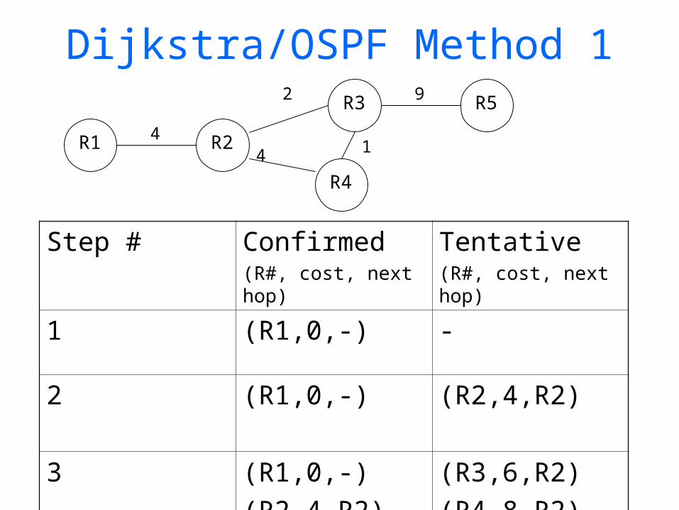
Dijkstra/OSPF Method 1
R1 R2
R4
R3 R5
4
2 9
4 1
Step # Confirmed(R#, cost, next hop)
Tentative(R#, cost, next hop)
1 (R1,0,-) -
2 (R1,0,-) (R2,4,R2)
3 (R1,0,-)(R2,4,R2)
(R3,6,R2)(R4,8,R2)
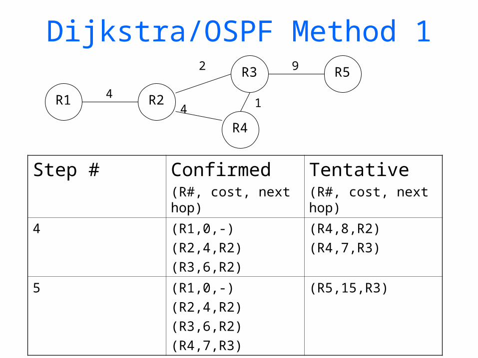
Dijkstra/OSPF Method 1
R1 R2
R4
R3 R5
4
2 9
4 1
Step # Confirmed(R#, cost, next hop)
Tentative(R#, cost, next hop)
4 (R1,0,-)(R2,4,R2)(R3,6,R2)
(R4,8,R2)(R4,7,R3)
5 (R1,0,-)(R2,4,R2)(R3,6,R2)(R4,7,R3)
(R5,15,R3)
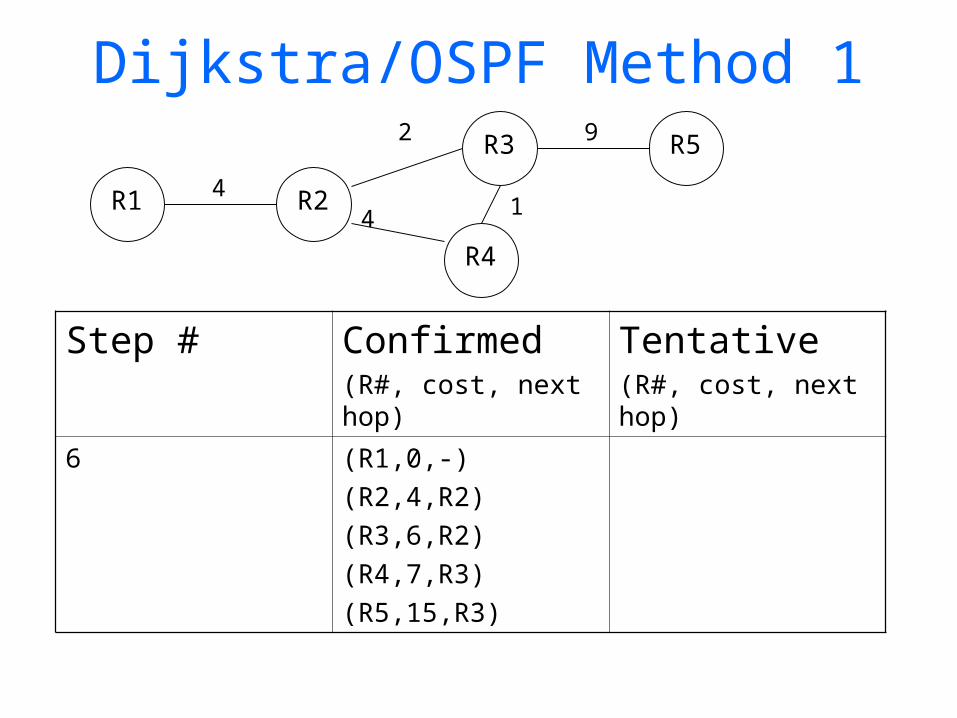
Dijkstra/OSPF Method 1
R1 R2
R4
R3 R5
4
2 9
4 1
Step # Confirmed(R#, cost, next hop)
Tentative(R#, cost, next hop)
6 (R1,0,-)(R2,4,R2)(R3,6,R2)(R4,7,R3)(R5,15,R3)

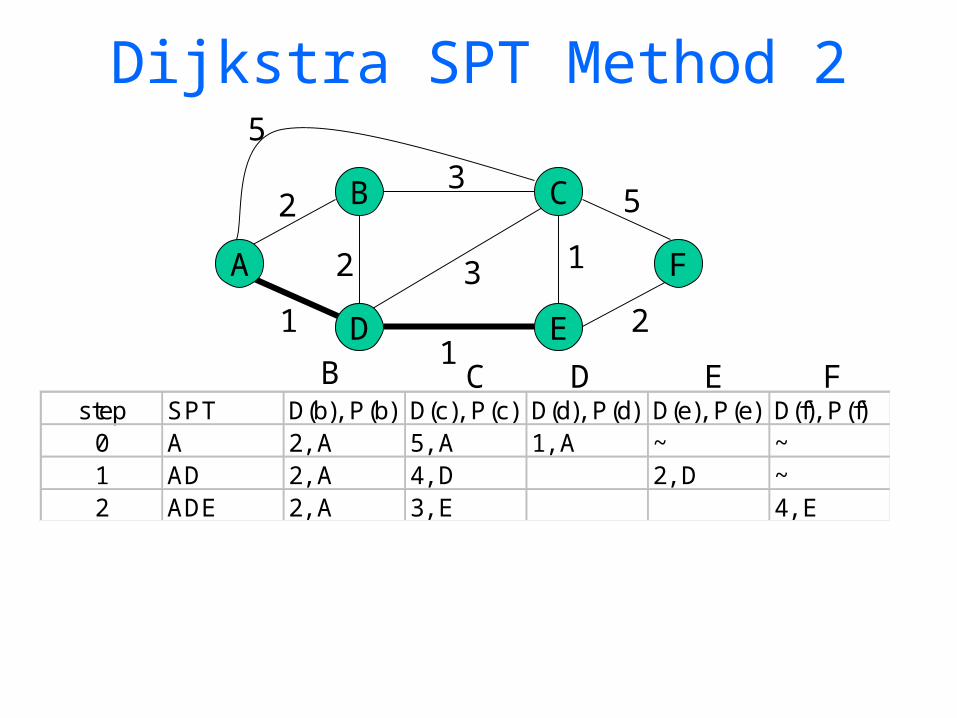
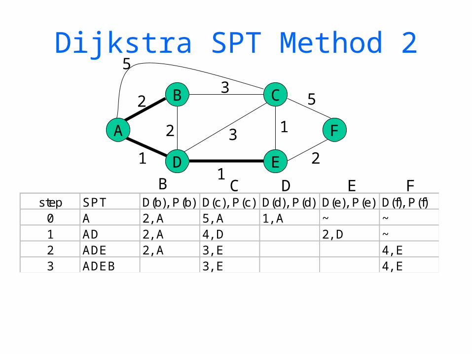
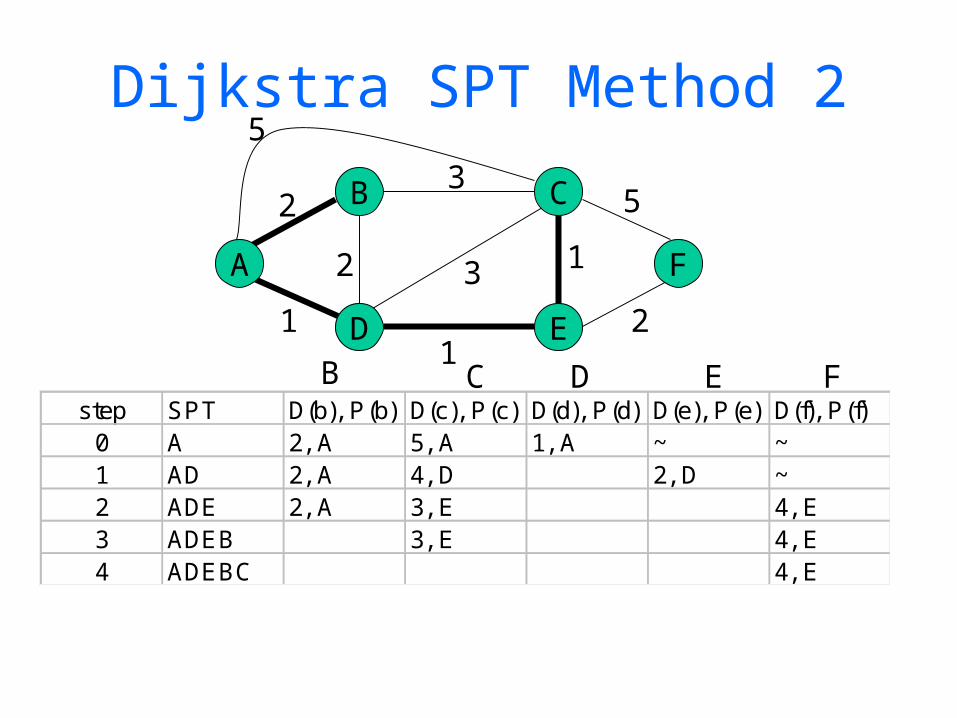
Dijkstra SPT Method 2
A F
B
D E
C2
2
2
3
1
1
1
3
5
step SPT D(b), P(b) D(c), P(c) D(d), P(d) D(e), P(e) D(f), P(f)0 A 2, A 5, A 1, A ~ ~
5
B C D E F

A F
B
D E
C2
2
2
3
1
1
1
3
5
step SPT D(b), P(b) D(c), P(c) D(d), P(d) D(e), P(e) D(f), P(f)0 A 2, A 5, A 1, A ~ ~1 AD 2, A 4, D 2, D ~
5
B C D E F
Dijkstra SPT Method 2
A F
B
D E
C2
2
2
3
1
1
1
3
5
step SPT D(b), P(b) D(c), P(c) D(d), P(d) D(e), P(e) D(f), P(f)0 A 2, A 5, A 1, A ~ ~1 AD 2, A 4, D 2, D ~2 ADE 2, A 3, E 4, E
5
B C D E F
Dijkstra SPT Method 2
A F
B
D E
C2
2
2
3
1
1
1
3
5
step SPT D(b), P(b) D(c), P(c) D(d), P(d) D(e), P(e) D(f), P(f)0 A 2, A 5, A 1, A ~ ~1 AD 2, A 4, D 2, D ~2 ADE 2, A 3, E 4, E3 ADEB 3, E 4, E
5
B C D E F
Dijkstra SPT Method 2
A F
B
D E
C2
2
2
3
1
1
1
3
5
step SPT D(b), P(b) D(c), P(c) D(d), P(d) D(e), P(e) D(f), P(f)0 A 2, A 5, A 1, A ~ ~1 AD 2, A 4, D 2, D ~2 ADE 2, A 3, E 4, E3 ADEB 3, E 4, E4 ADEBC 4, E
5
B C D E F
Dijkstra SPT Method 2

A F
B
D E
C2
2
2
3
1
1
1
3
5
step SPT D(b), P(b) D(c), P(c) D(d), P(d) D(e), P(e) D(f), P(f)0 A 2, A 5, A 1, A ~ ~1 AD 2, A 4, D 2, D ~2 ADE 2, A 3, E 4, E3 ADEB 3, E 4, E4 ADEBC 4, E5 ADEBCF
5
B C D E F
Dijkstra SPT Method 2
Link State in Practice
• OSPF (Open Shortest Path First Protocol)– most commonly used routing protocol
in the Internet– support for authentication, addl
hierarchy, load balancing
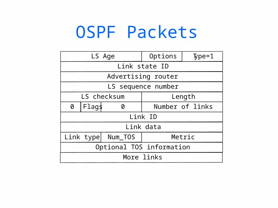
OSPF PacketsLS Age Options Type=1
0 Flags 0 Number of links
Link type Num_TOS Metric
Link state ID
Advertising router
LS sequence number
Link ID
Link data
Optional TOS information
More links
LS checksum Length
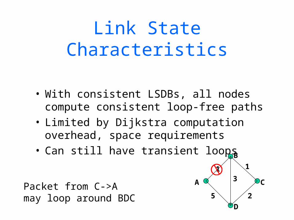
Link State Characteristics
• With consistent LSDBs, all nodes compute consistent loop-free paths
• Limited by Dijkstra computation overhead, space requirements
• Can still have transient loops
A
B
C
D
13
5 2
1
Packet from C->Amay loop around BDC
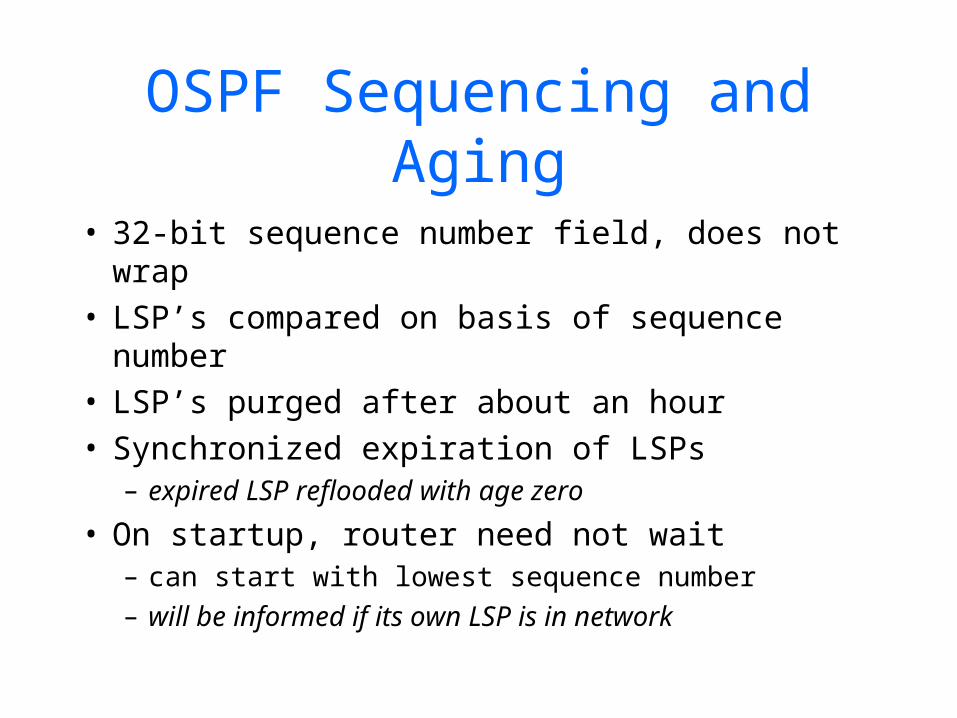
OSPF Sequencing and Aging
• 32-bit sequence number field, does not wrap• LSP’s compared on basis of sequence
number• LSP’s purged after about an hour• Synchronized expiration of LSPs
– expired LSP reflooded with age zero
• On startup, router need not wait– can start with lowest sequence number– will be informed if its own LSP is in network

Problem: Router Failure
• A failed router and comes up but does not remember the last sequence number it used before it crashed
• New LSPs may be ignored if they have lower sequence number
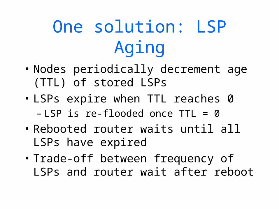
One solution: LSP Aging
• Nodes periodically decrement age (TTL) of stored LSPs
• LSPs expire when TTL reaches 0– LSP is re-flooded once TTL = 0
• Rebooted router waits until all LSPs have expired
• Trade-off between frequency of LSPs and router wait after reboot
69
Today’s Homework• Peterson & Davie, Chap 4
-4.12-4.13-4.16-4.21Download and browse RIP and OSPF RFC’s
Due on Fri (2/29)