ECE544: Communication Networks-II Spring 2009 H. Liu Lecture 4 Includes teaching materials from D....
73
ECE544: Communication Networks-II Spring 2009 H. Liu Lecture 4 Includes teaching materials from D. Raychaudhuri, L. Peterson
-
date post
21-Dec-2015 -
Category
Documents
-
view
213 -
download
0
Transcript of ECE544: Communication Networks-II Spring 2009 H. Liu Lecture 4 Includes teaching materials from D....
ECE544: Communication Networks-II Spring 2009
H. Liu
Lecture 4
Includes teaching materials from D. Raychaudhuri, L. Peterson
Today’s Lecture
• IP basics• Routing principles
– distance vector (RIP)– link state (OSPF)
IP Basics
Best Effort Service ModelGlobal Addressing SchemeARP & DHCP
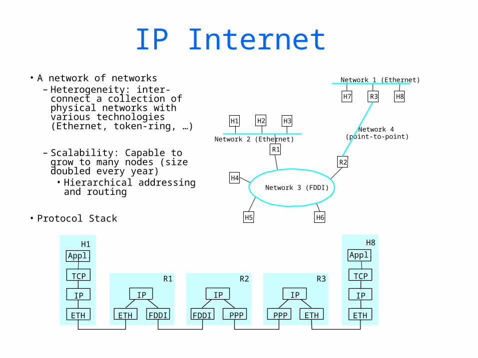
IP Internet • A network of networks
– Heterogeneity: inter-connect a collection of physical networks with various technologies (Ethernet, token-ring, …)
– Scalability: Capable to grow to many nodes (size doubled every year)• Hierarchical addressing and
routing
• Protocol Stack
R2
R1
H4
H5
H3H2H1
Network 2 (Ethernet)
Network 1 (Ethernet)
H6
Network 3 (FDDI)
Network 4(point-to-point)
H7 R3 H8
R1
ETH FDDI
IPIP
ETH
TCP R2
FDDI PPP
IP
R3
PPP ETH
IP
H1
IP
ETH
TCP
H8
Appl. Appl.
Service Model
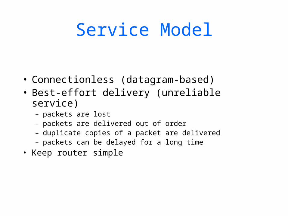
• Connectionless (datagram-based)• Best-effort delivery (unreliable service)
– packets are lost– packets are delivered out of order– duplicate copies of a packet are delivered– packets can be delayed for a long time
• Keep router simple
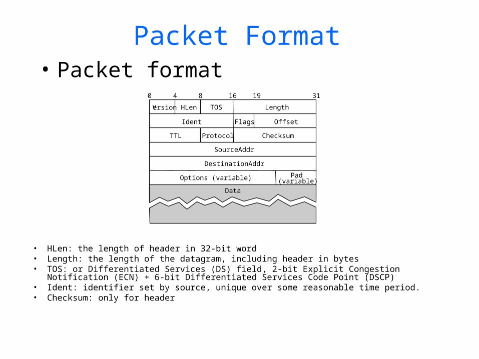
Packet Format• Packet format
Version HLen TOS Length
Ident Flags Offset
TTL Protocol Checksum
SourceAddr
DestinationAddr
Options (variable) Pad(variable)
0 4 8 16 19 31
Data
• HLen: the length of header in 32-bit word• Length: the length of the datagram, including header in bytes• TOS: or Differentiated Services (DS) field, 2-bit Explicit Congestion Notification (ECN) +
6-bit Differentiated Services Code Point (DSCP)• Ident: identifier set by source, unique over some reasonable time period.• Checksum: only for header
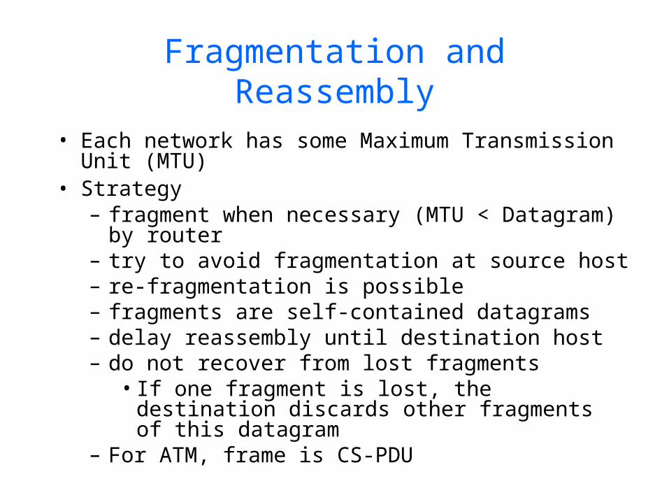
Fragmentation and Reassembly
• Each network has some Maximum Transmission Unit (MTU)
• Strategy– fragment when necessary (MTU < Datagram)
by router– try to avoid fragmentation at source host– re-fragmentation is possible – fragments are self-contained datagrams– delay reassembly until destination host– do not recover from lost fragments
• If one fragment is lost, the destination discards other fragments of this datagram
– For ATM, frame is CS-PDU
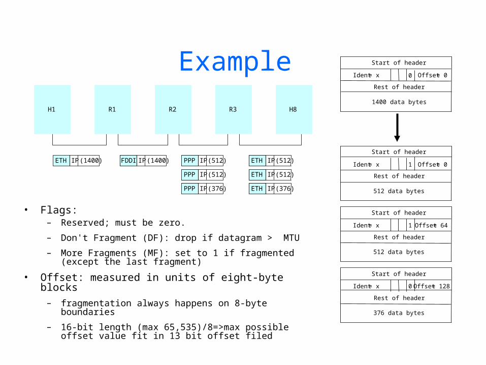
Example
H1 R1 R2 R3 H8
ETH IP (1400) FDDI IP (1400) PPP IP (512)
PPP IP (376)
PPP IP (512)
ETH IP (512)
ETH IP (376)
ETH IP (512)
Ident = x Offset = 0
Start of header
0
Rest of header
1400 data bytes
Ident = x Offset = 0
Start of header
1
Rest of header
512 data bytes
Ident = x Offset = 64
Start of header
1
Rest of header
512 data bytes
Ident = x Offset = 128
Start of header
0
Rest of header
376 data bytes
• Flags:– Reserved; must be zero.
– Don't Fragment (DF): drop if datagram > MTU
– More Fragments (MF): set to 1 if fragmented (except the last fragment)
• Offset: measured in units of eight-byte blocks– fragmentation always happens on 8-byte boundaries
– 16-bit length (max 65,535)/8=>max possible offset value fit in 13 bit offset filed
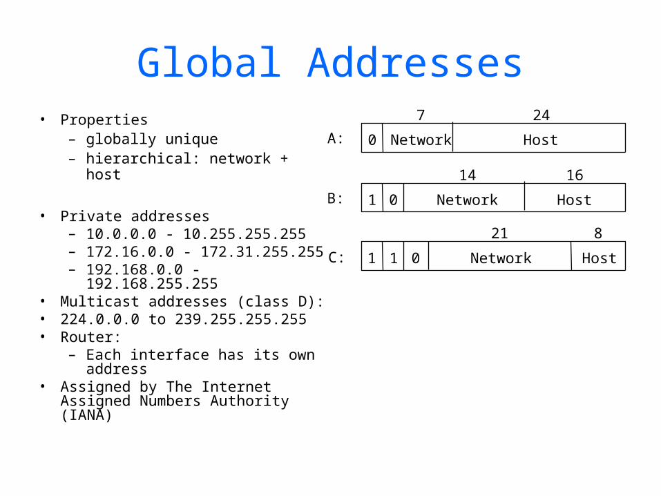
Global Addresses• Properties
– globally unique– hierarchical: network + host
• Private addresses– 10.0.0.0 - 10.255.255.255– 172.16.0.0 - 172.31.255.255– 192.168.0.0 -
192.168.255.255 • Multicast addresses (class D): • 224.0.0.0 to 239.255.255.255• Router:
– Each interface has its own address
• Assigned by The Internet Assigned Numbers Authority (IANA)
Network Host
7 24
0A:
Network Host
14 16
1 0B:
Network Host
21 8
1 1 0C:
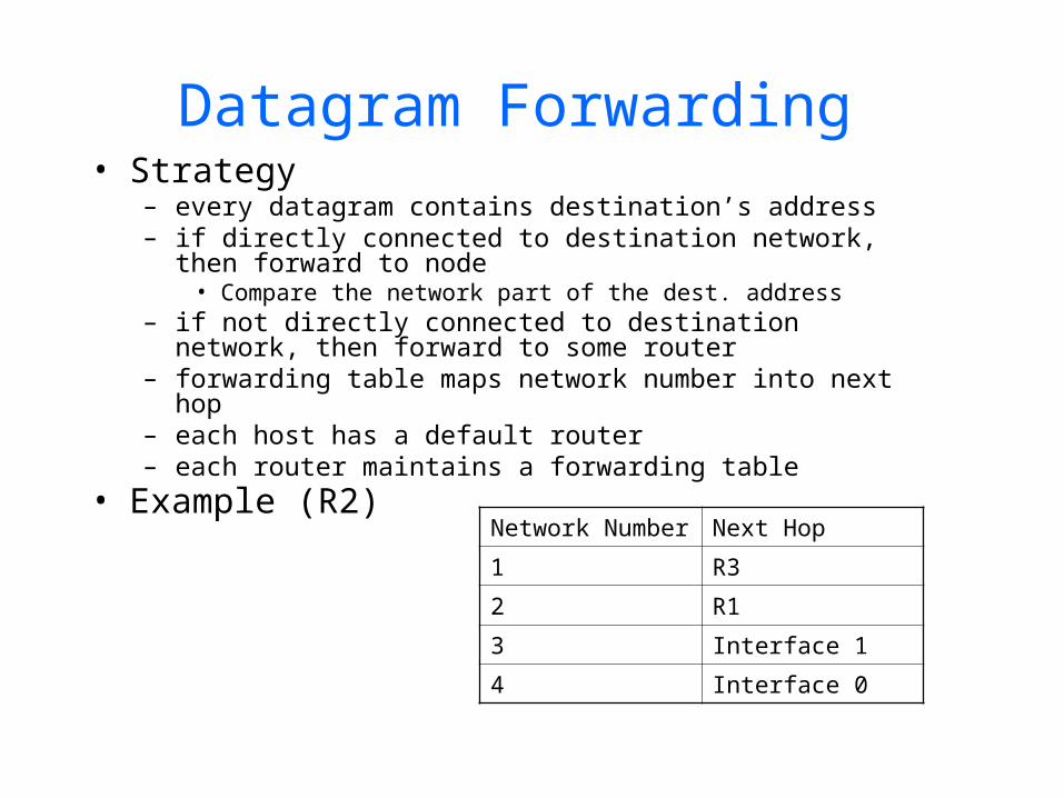
Datagram Forwarding • Strategy
– every datagram contains destination’s address– if directly connected to destination network, then
forward to node• Compare the network part of the dest. address
– if not directly connected to destination network, then forward to some router
– forwarding table maps network number into next hop– each host has a default router– each router maintains a forwarding table
• Example (R2) Network Number Next Hop
1 R3
2 R1
3 Interface 1
4 Interface 0
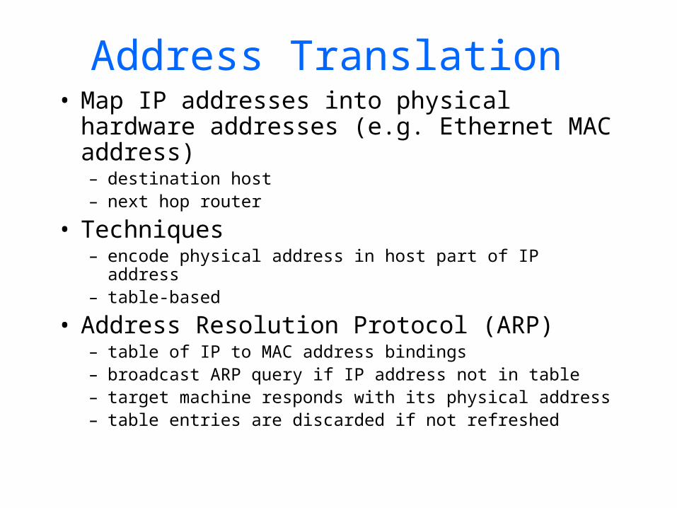
Address Translation • Map IP addresses into physical
hardware addresses (e.g. Ethernet MAC address)– destination host– next hop router
• Techniques– encode physical address in host part of IP address– table-based
• Address Resolution Protocol (ARP)– table of IP to MAC address bindings– broadcast ARP query if IP address not in table– target machine responds with its physical address– table entries are discarded if not refreshed
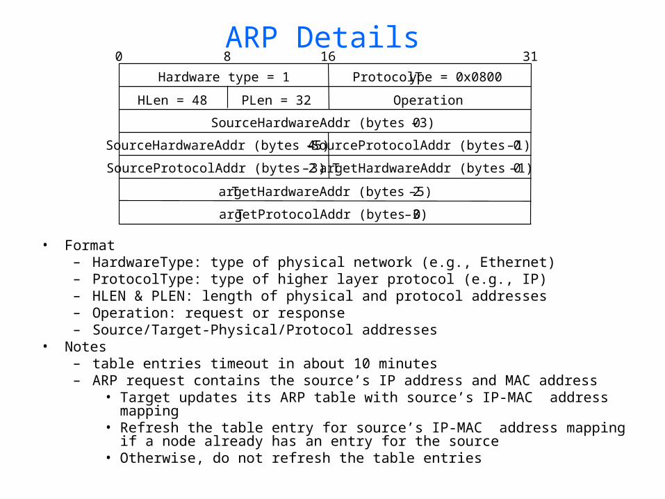
ARP Details
• Format– HardwareType: type of physical network (e.g., Ethernet)– ProtocolType: type of higher layer protocol (e.g., IP)– HLEN & PLEN: length of physical and protocol addresses– Operation: request or response – Source/Target-Physical/Protocol addresses
• Notes– table entries timeout in about 10 minutes– ARP request contains the source’s IP address and MAC address
• Target updates its ARP table with source’s IP-MAC address mapping
• Refresh the table entry for source’s IP-MAC address mapping if a node already has an entry for the source
• Otherwise, do not refresh the table entries
TargetHardwareAddr (bytes 2 – 5)
TargetProtocolAddr (bytes 0 – 3)
SourceProtocolAddr (bytes 2 – 3)
Hardware type = 1 ProtocolType = 0x0800
SourceHardwareAddr (bytes 4 – 5)
TargetHardwareAddr (bytes 0 – 1)
SourceProtocolAddr (bytes 0 – 1)
HLen = 48 PLen = 32 Operation
SourceHardwareAddr (bytes 0 – 3)
0 8 16 31
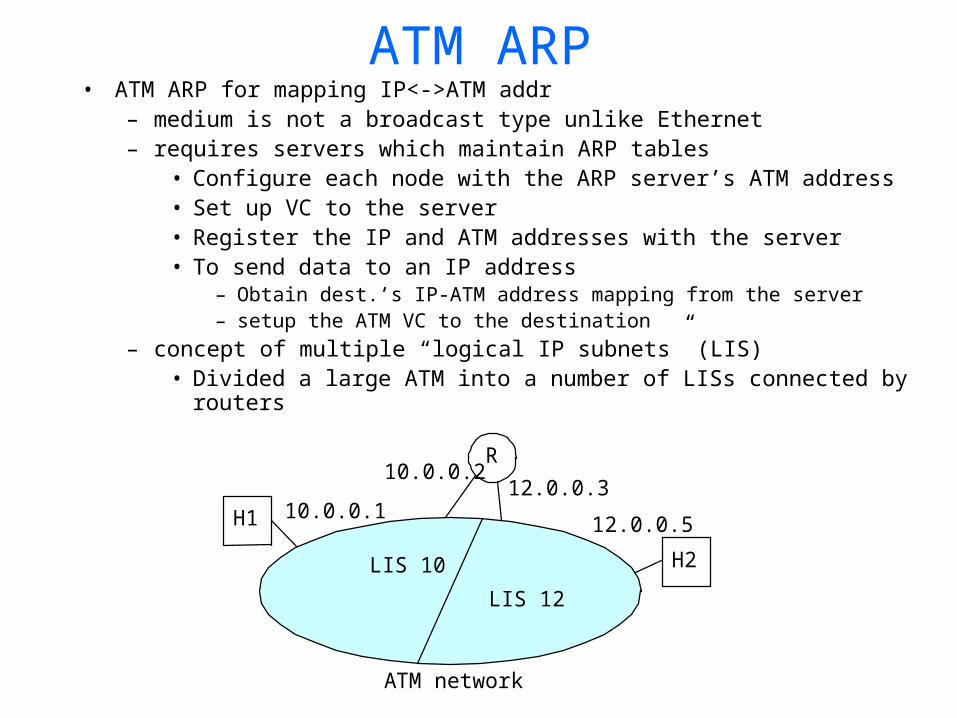
ATM ARP
H2
R
H1
LIS 10
LIS 12
ATM network
10.0.0.2
10.0.0.112.0.0.3
12.0.0.5
• ATM ARP for mapping IP<->ATM addr– medium is not a broadcast type unlike Ethernet– requires servers which maintain ARP tables
• Configure each node with the ARP server’s ATM address• Set up VC to the server• Register the IP and ATM addresses with the server • To send data to an IP address
– Obtain dest.’s IP-ATM address mapping from the server – setup the ATM VC to the destination
– concept of multiple “logical IP subnets” (LIS)• Divided a large ATM into a number of LISs connected by
routers
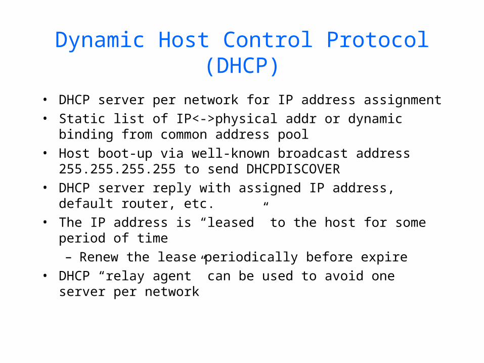
Dynamic Host Control Protocol (DHCP)
• DHCP server per network for IP address assignment• Static list of IP<->physical addr or dynamic binding
from common address pool• Host boot-up via well-known broadcast address
255.255.255.255 to send DHCPDISCOVER• DHCP server reply with assigned IP address, default
router, etc.• The IP address is “leased” to the host for some period of
time– Renew the lease periodically before expire
• DHCP “relay agent” can be used to avoid one server per network
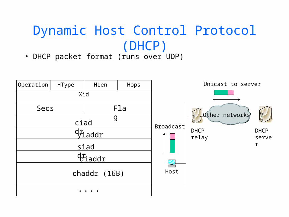
Dynamic Host Control Protocol (DHCP)
• DHCP packet format (runs over UDP)
Operation HType HLen Hops
Xid
Secs Flag
ciaddr
yiaddr
siaddr
giaddr
chaddr (16B)
....
Host
Other networks
Unicast to server
BroadcastDHCP relay
DHCP server
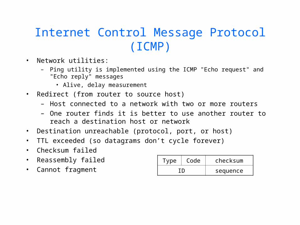
Internet Control Message Protocol (ICMP)
• Network utilities: – Ping utility is implemented using the ICMP "Echo request" and "Echo reply"
messages• Alive, delay measurement
• Redirect (from router to source host)– Host connected to a network with two or more routers– One router finds it is better to use another router to reach a
destination host or network• Destination unreachable (protocol, port, or host)• TTL exceeded (so datagrams don’t cycle forever)• Checksum failed • Reassembly failed• Cannot fragment
Type Code checksum
ID sequence
Routing Basics
Routing Problem• Routing Problem: How to find the lowest cost path between two
nodes – the process to build the routing and forwarding tables in each
router• Network as a Graph
– Each edge has a cost– Path cost = the sum of the costs of all the edges that make up
the path. • Factors
– dynamic: link, node, topology, link cost changes
4
3
6
21
9
1
1D
A
FE
B
C
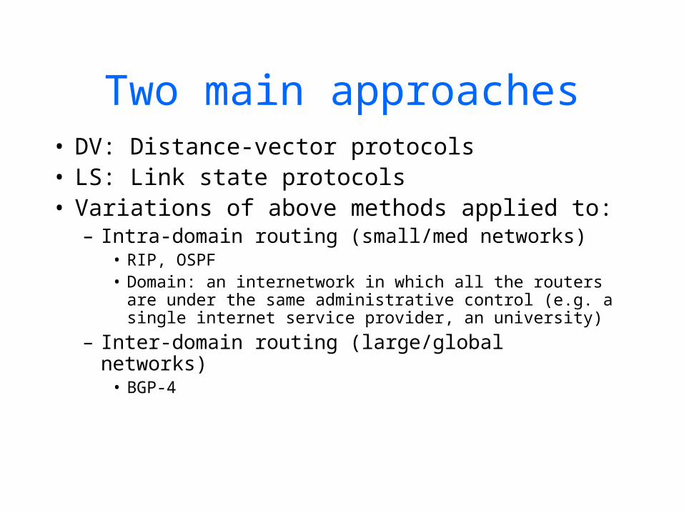
Two main approaches• DV: Distance-vector protocols• LS: Link state protocols• Variations of above methods applied to:
– Intra-domain routing (small/med networks)• RIP, OSPF• Domain: an internetwork in which all the routers
are under the same administrative control (e.g. a single internet service provider, an university)
– Inter-domain routing (large/global networks)• BGP-4
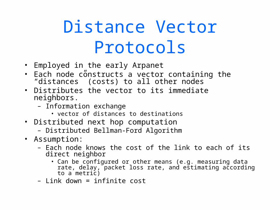
Distance Vector Protocols• Employed in the early Arpanet• Each node constructs a vector containing the
“distances” (costs) to all other nodes• Distributes the vector to its immediate neighbors.
– Information exchange • vector of distances to destinations
• Distributed next hop computation– Distributed Bellman-Ford Algorithm
• Assumption:– Each node knows the cost of the link to each of its direct
neighbor• Can be configured or other means (e.g. measuring data rate,
delay, packet loss rate, and estimating according to a metric)– Link down = infinite cost
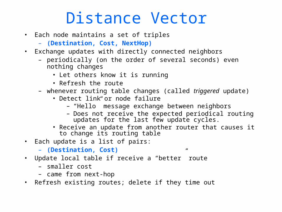
Distance Vector • Each node maintains a set of triples
– (Destination, Cost, NextHop)• Exchange updates with directly connected neighbors
– periodically (on the order of several seconds) even nothing changes
• Let others know it is running• Refresh the route
– whenever routing table changes (called triggered update)• Detect link or node failure
– “Hello” message exchange between neighbors– Does not receive the expected periodical routing updates
for the last few update cycles.• Receive an update from another router that causes it to
change its routing table• Each update is a list of pairs:
– (Destination, Cost)• Update local table if receive a “better” route
– smaller cost– came from next-hop
• Refresh existing routes; delete if they time out
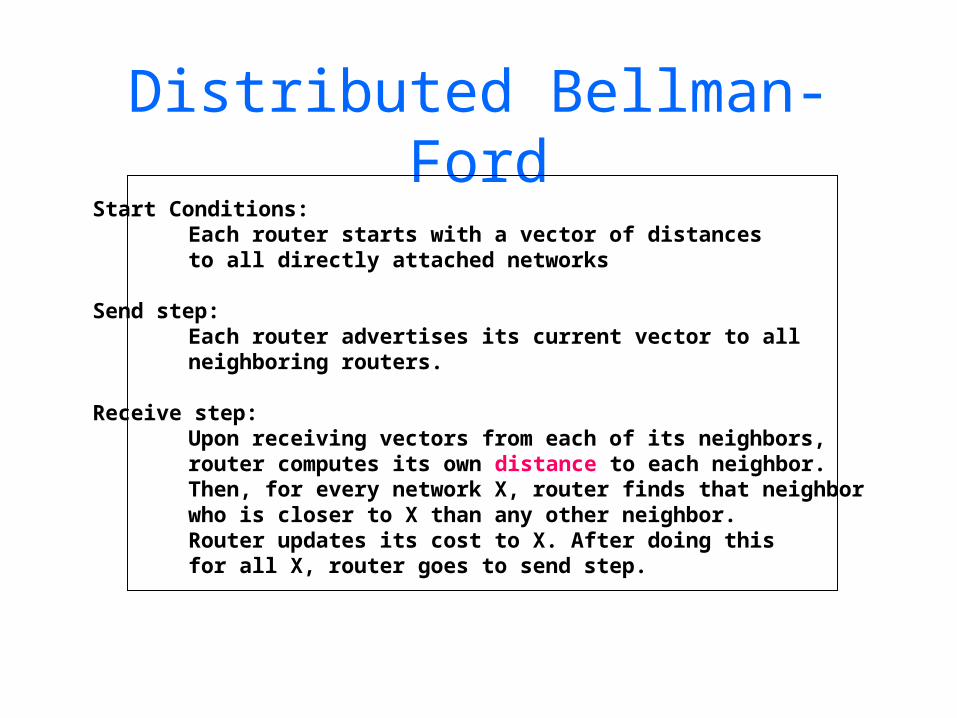
Distributed Bellman-FordStart Conditions:
Each router starts with a vector of distancesto all directly attached networks
Send step:Each router advertises its current vector to allneighboring routers.
Receive step:Upon receiving vectors from each of its neighbors,router computes its own distance to each neighbor.Then, for every network X, router finds that neighborwho is closer to X than any other neighbor.Router updates its cost to X. After doing thisfor all X, router goes to send step.
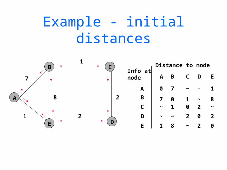
Example - initial distances
A
B
E
C
D
Info atnode
A
B
C
D
A B C
0 7 ~
7 0 1~ 1 0
~ ~ 2
7
1
1
2
28
Distance to node
D
~
~2
0
E 1 8 ~ 2
1
8~
2
0
E
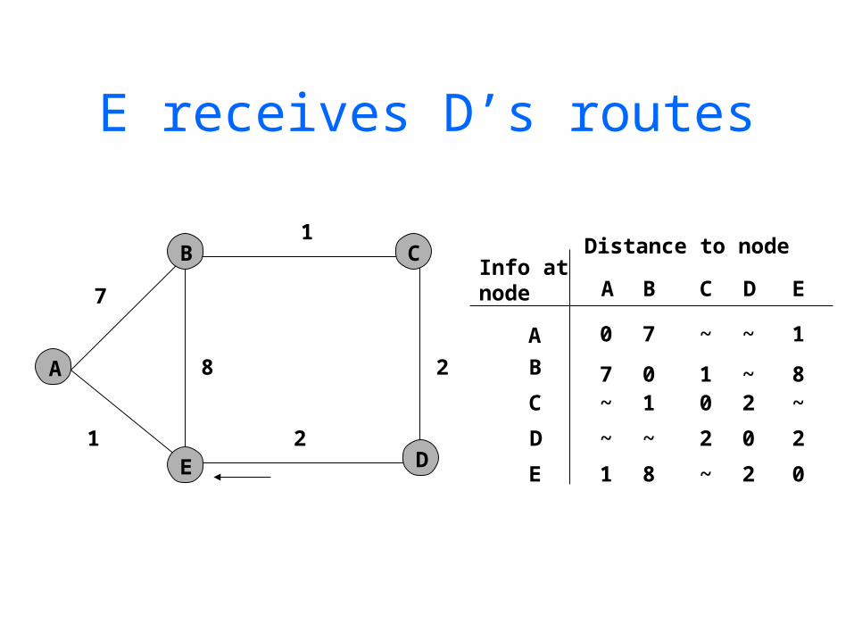
E receives D’s routes
A
B
E
C
D
Info atnode
A
B
C
D
A B C
0 7 ~
7 0 1~ 1 0
~ ~ 2
7
1
1
2
28
Distance to node
D
~
~2
0
E 1 8 ~ 2
1
8~
2
0
E
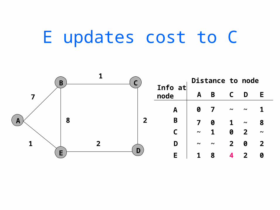
E updates cost to C
A
B
E
C
D
Info atnode
A
B
C
D
A B C
0 7 ~
7 0 1~ 1 0
~ ~ 2
7
1
1
2
28
Distance to node
D
~
~2
0
E 1 8 4 2
1
8~
2
0
E
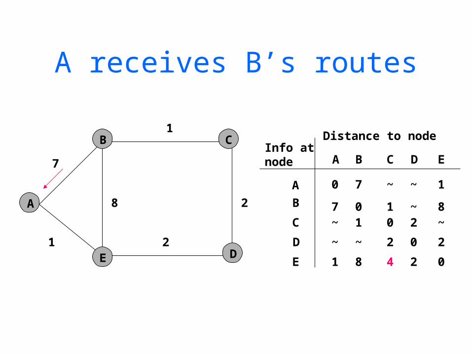
A receives B’s routes
A
B
E
C
D
Info atnode
A
B
C
D
A B C
0 7 ~
7 0 1~ 1 0
~ ~ 2
7
1
1
2
28
Distance to node
D
~
~2
0
E 1 8 4 2
1
8~
2
0
E
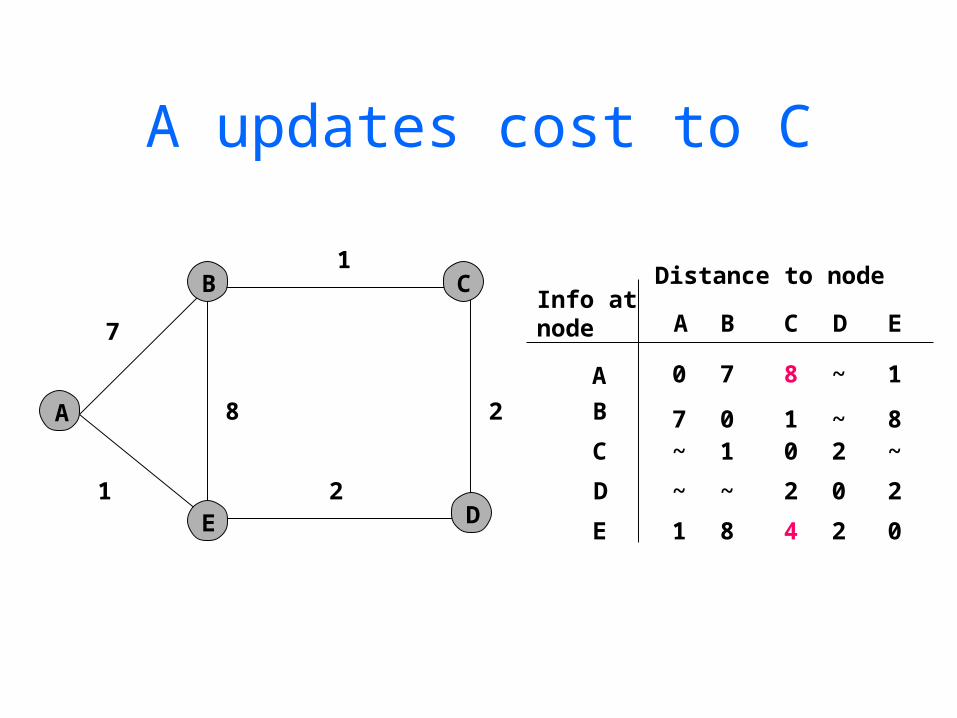
A updates cost to C
A
B
E
C
D
Info atnode
A
B
C
D
A B C
0 7 8
7 0 1~ 1 0
~ ~ 2
7
1
1
2
28
Distance to node
D
~
~2
0
E 1 8 4 2
1
8~
2
0
E
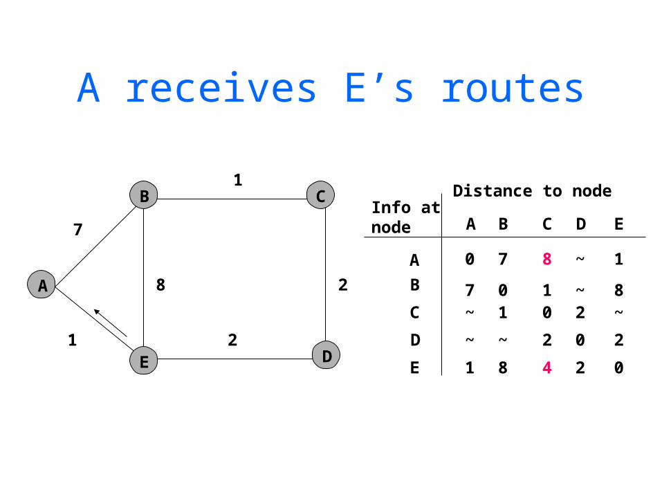
A receives E’s routes
A
B
E
C
D
Info atnode
A
B
C
D
A B C
0 7 8
7 0 1~ 1 0
~ ~ 2
7
1
1
2
28
Distance to node
D
~
~2
0
E 1 8 4 2
1
8~
2
0
E
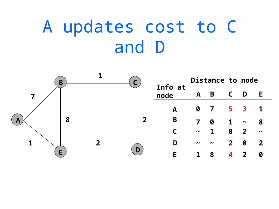
A updates cost to C and D
A
B
E
C
D
Info atnode
A
B
C
D
A B C
0 7 5
7 0 1~ 1 0
~ ~ 2
7
1
1
2
28
Distance to node
D
3
~2
0
E 1 8 4 2
1
8~
2
0
E
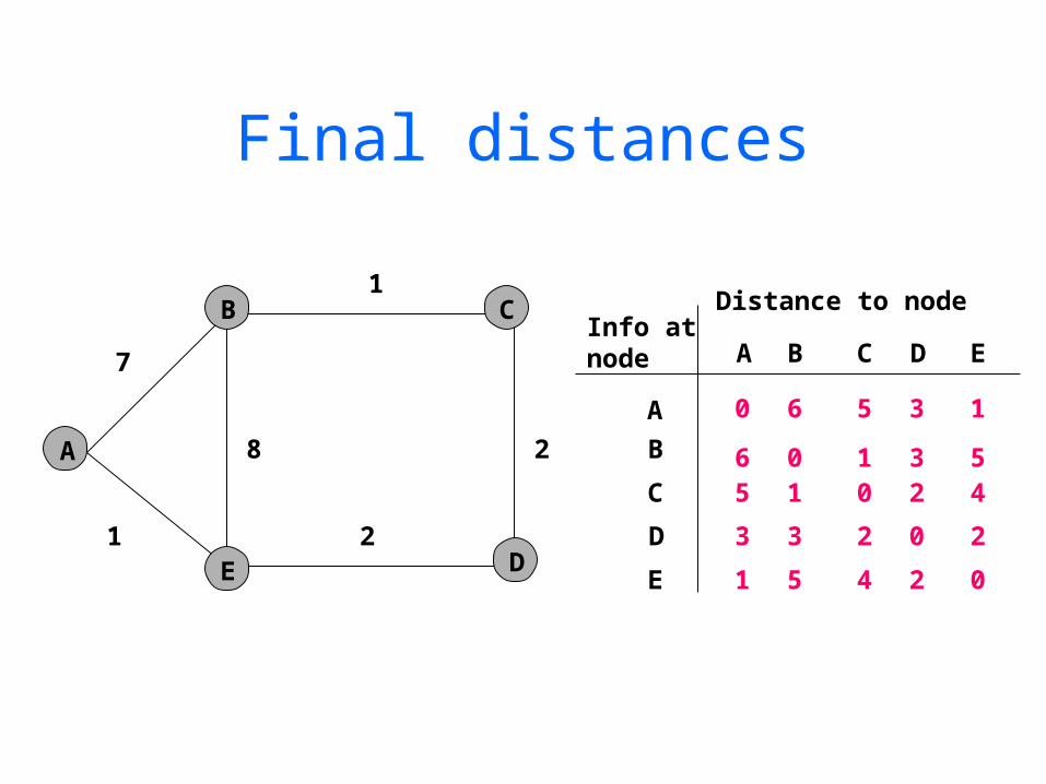
Final distances
A
B C
D
Info atnode
A
B
C
D
A B C
0 6 5
6 0 15 1 0
3 3 2
7
1
1
2
28
Distance to node
D
3
32
0
E 1 5 4 2
1
54
2
0
E
E
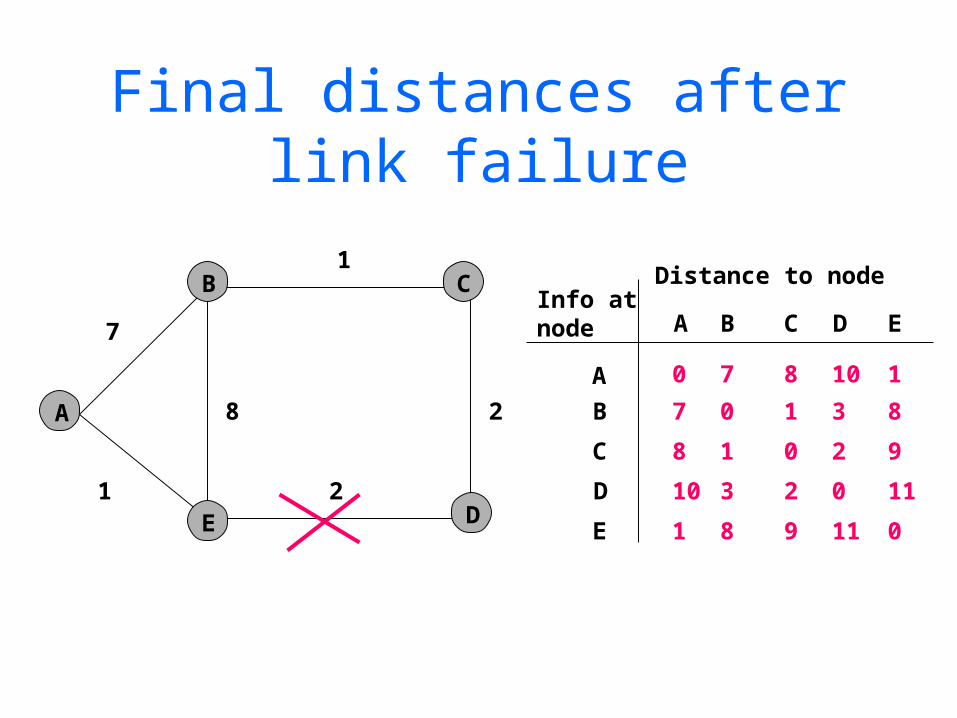
Final distances after link failure
A
B C
D
Info atnode
A
B
C
D
A B C
0 7 8
7 0 1
8 1 0
10 3 2
7
1
1
2
28
Distance to node
D
10
3
2
0
E 1 8 9 11
1
8
9
11
0
E
E
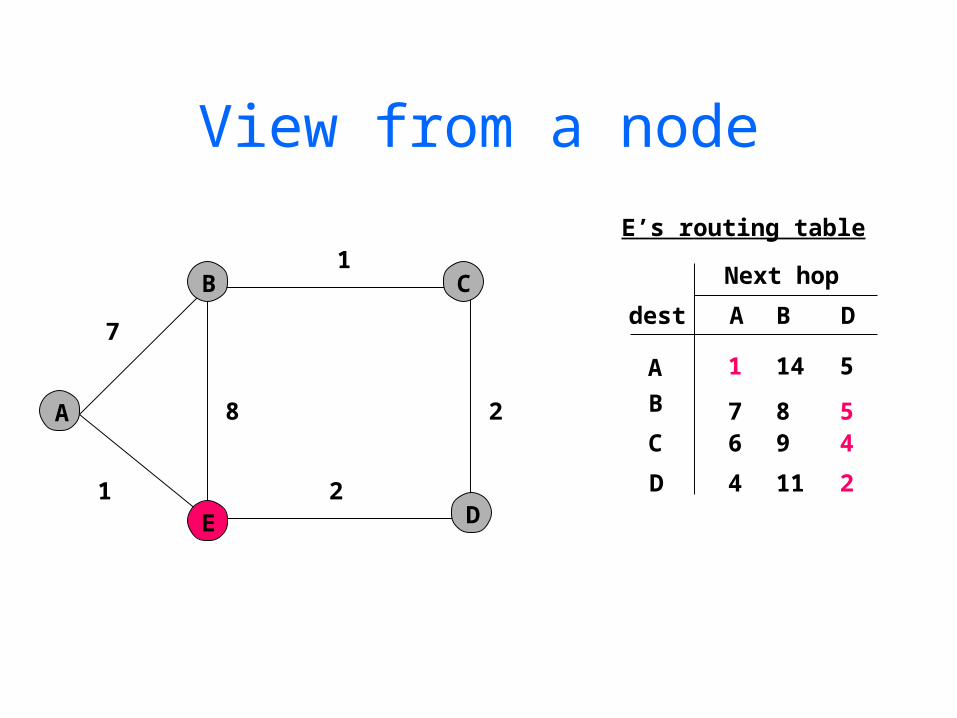
View from a node
A
B
E
C
D
dest
A
B
C
D
A B D
1 14 5
7 8 56 9 4
4 11 2
7
1
1
2
28
Next hop
E’s routing table
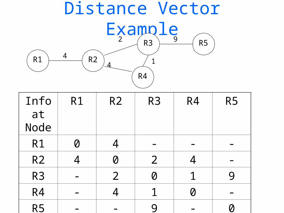
Distance Vector Example
R1 R2
R4
R3 R5
4
2 9
4 1
Info at
Node
R1 R2 R3 R4 R5
R1 0 4 - - -
R2 4 0 2 4 -
R3 - 2 0 1 9
R4 - 4 1 0 -
R5 - - 9 - 0
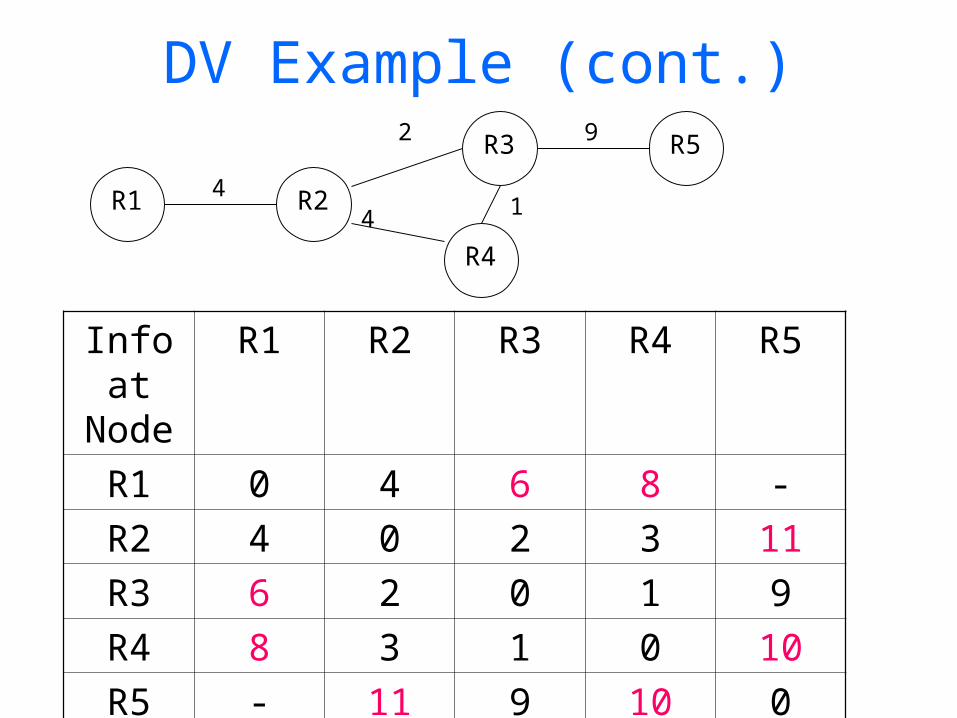
DV Example (cont.)
R1 R2
R4
R3 R5
4
2 9
4 1
Info at
Node
R1 R2 R3 R4 R5
R1 0 4 6 8 -
R2 4 0 2 3 11
R3 6 2 0 1 9
R4 8 3 1 0 10
R5 - 11 9 10 0
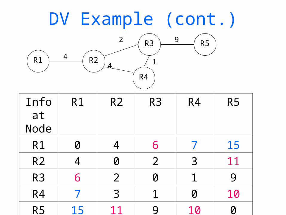
DV Example (cont.)
R1 R2
R4
R3 R5
4
2 9
4 1
Info at
Node
R1 R2 R3 R4 R5
R1 0 4 6 7 15
R2 4 0 2 3 11
R3 6 2 0 1 9
R4 7 3 1 0 10
R5 15 11 9 10 0
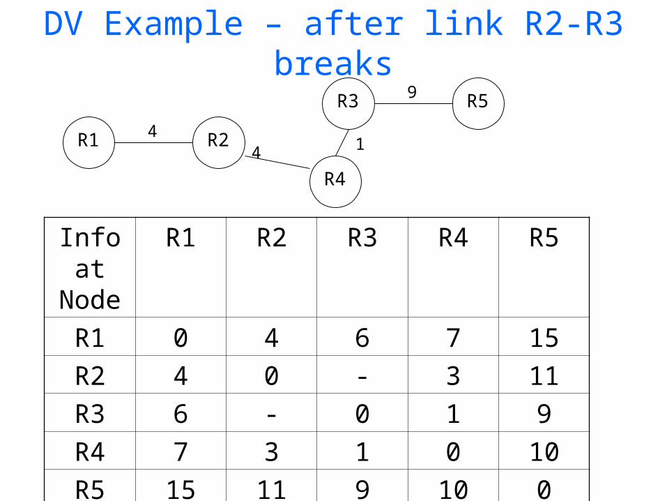
DV Example – after link R2-R3 breaks
R1 R2
R4
R3 R5
4
9
4 1
Info at
Node
R1 R2 R3 R4 R5
R1 0 4 6 7 15
R2 4 0 - 3 11
R3 6 - 0 1 9
R4 7 3 1 0 10
R5 15 11 9 10 0
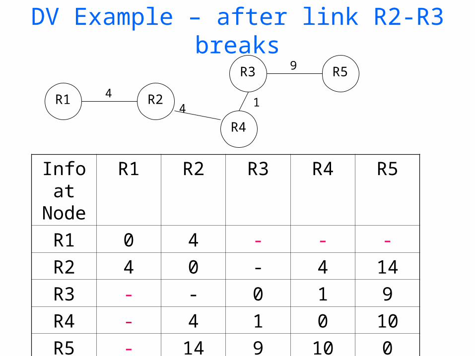
DV Example – after link R2-R3 breaks
R1 R2
R4
R3 R5
4
9
4 1
Info at
Node
R1 R2 R3 R4 R5
R1 0 4 - - -
R2 4 0 - 4 14
R3 - - 0 1 9
R4 - 4 1 0 10
R5 - 14 9 10 0
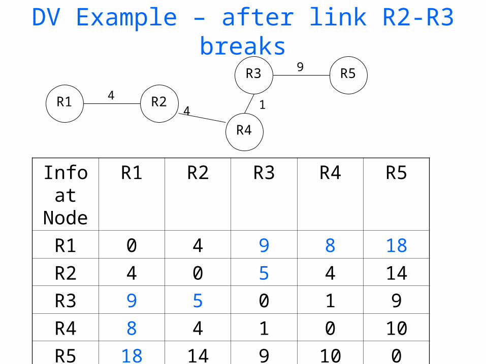
DV Example – after link R2-R3 breaks
R1 R2
R4
R3 R5
4
9
4 1
Info at
Node
R1 R2 R3 R4 R5
R1 0 4 9 8 18
R2 4 0 5 4 14
R3 9 5 0 1 9
R4 8 4 1 0 10
R5 18 14 9 10 0
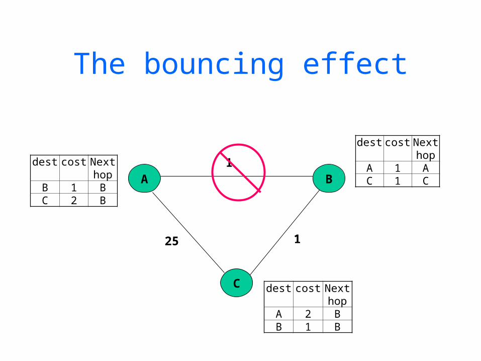
The bouncing effect
dest cost Next hop
B 1 BC 2 B
dest cost Next hop
A 1 AC 1 CA
25
1
1
B
C dest cost Next hop
A 2 BB 1 B
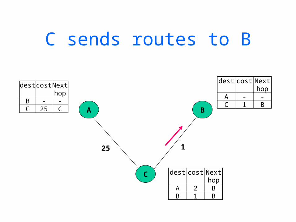
C sends routes to B
A
25 1
B
C
dest cost Next hop
B - -C 25 C
dest cost Next hop
A 2 BB 1 B
dest cost Next hop
A - -C 1 B
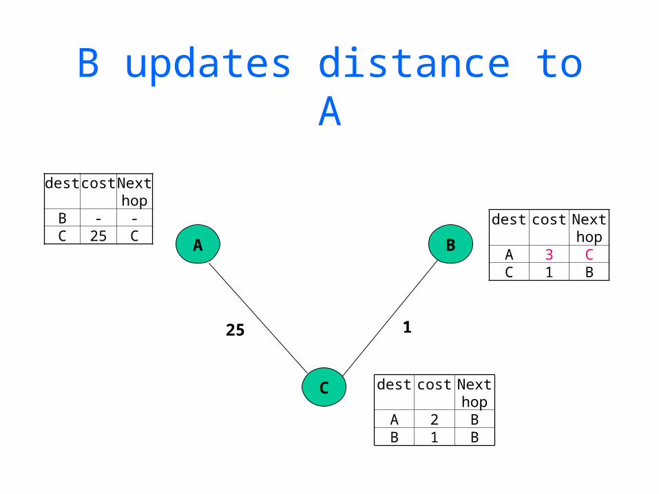
B updates distance to A
A
25 1
B
C
dest cost Next hop
A 3 CC 1 B
dest cost Next hop
A 2 BB 1 B
dest cost Next hop
B - -C 25 C
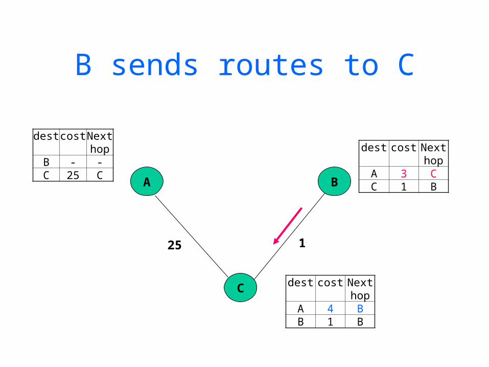
B sends routes to C
A
25 1
B
C
dest cost Next hop
B - -C 25 C
dest cost Next hop
A 3 CC 1 B
dest cost Next hop
A 4 BB 1 B
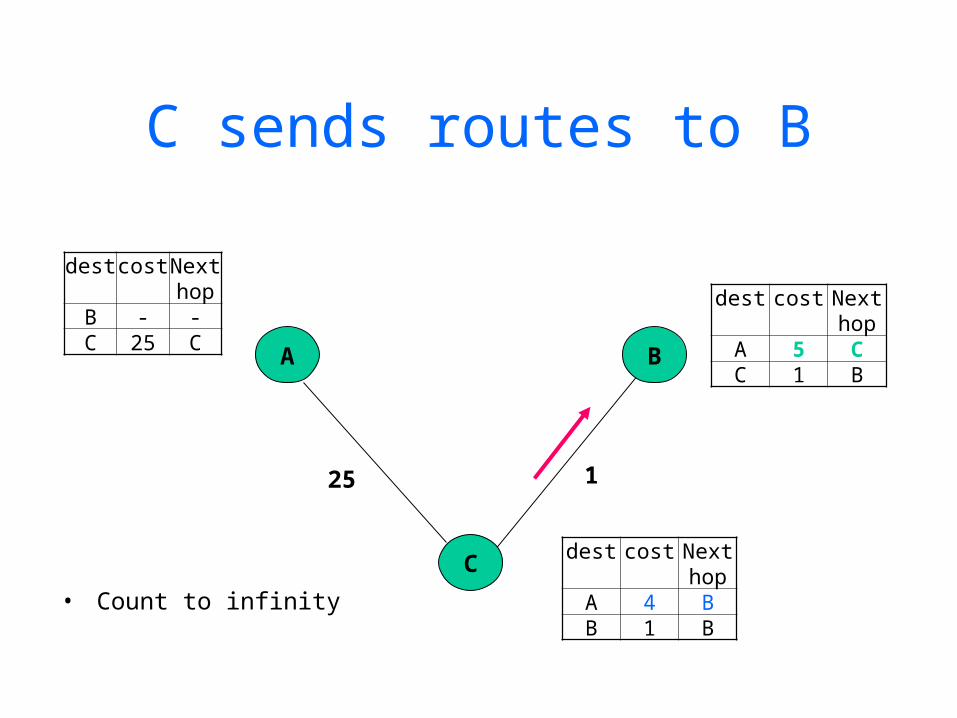
C sends routes to B
A
25 1
B
C
• Count to infinity
dest cost Next hop
B - -C 25 C
dest cost Next hop
A 4 BB 1 B
dest cost Next hop
A 5 CC 1 B
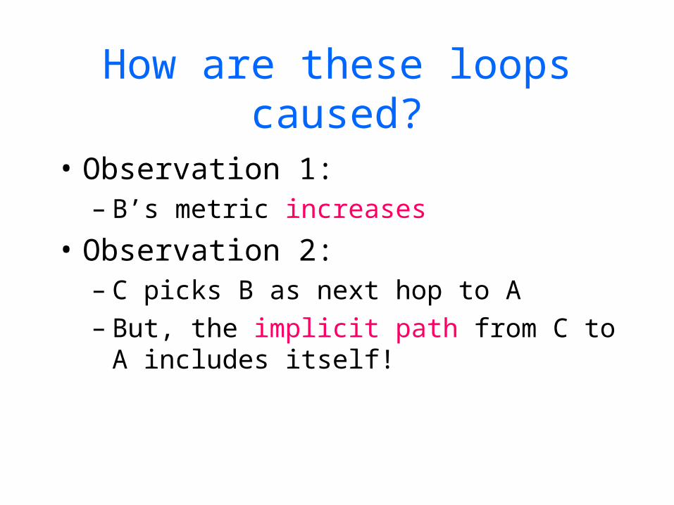
How are these loops caused?
• Observation 1:– B’s metric increases
• Observation 2:– C picks B as next hop to A– But, the implicit path from C to A
includes itself!
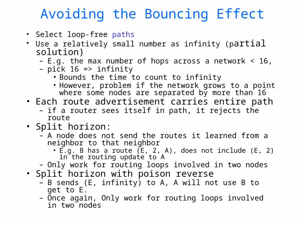
Avoiding the Bouncing Effect• Select loop-free paths• Use a relatively small number as infinity (partial
solution)– E.g. the max number of hops across a network < 16, – pick 16 => infinity
• Bounds the time to count to infinity• However, problem if the network grows to a point
where some nodes are separated by more than 16• Each route advertisement carries entire path
– if a router sees itself in path, it rejects the route• Split horizon:
– A node does not send the routes it learned from a neighbor to that neighbor
• E.g. B has a route (E, 2, A), does not include (E, 2) in the routing update to A
– Only work for routing loops involved in two nodes• Split horizon with poison reverse
– B sends (E, infinity) to A, A will not use B to get to E.– Once again, Only work for routing loops involved in
two nodes
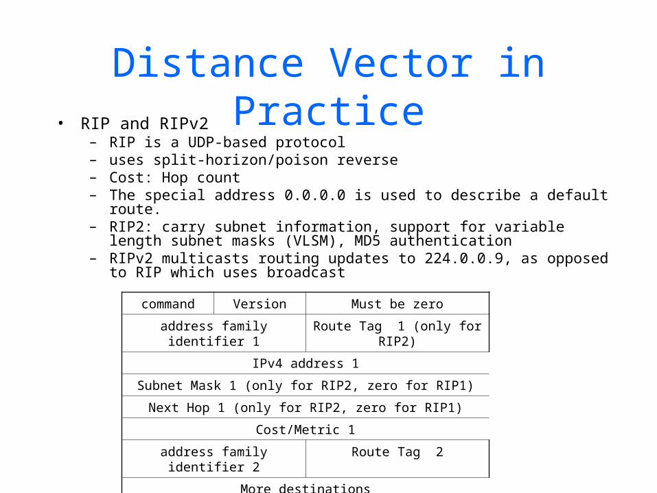
Distance Vector in Practice• RIP and RIPv2
– RIP is a UDP-based protocol– uses split-horizon/poison reverse– Cost: Hop count– The special address 0.0.0.0 is used to describe a default route.– RIP2: carry subnet information, support for variable length subnet
masks (VLSM), MD5 authentication– RIPv2 multicasts routing updates to 224.0.0.9, as opposed to RIP
which uses broadcast
command Version Must be zero
address family identifier 1 Route Tag 1 (only for RIP2)
IPv4 address 1
Subnet Mask 1 (only for RIP2, zero for RIP1)
Next Hop 1 (only for RIP2, zero for RIP1)
Cost/Metric 1
address family identifier 2 Route Tag 2
More destinations
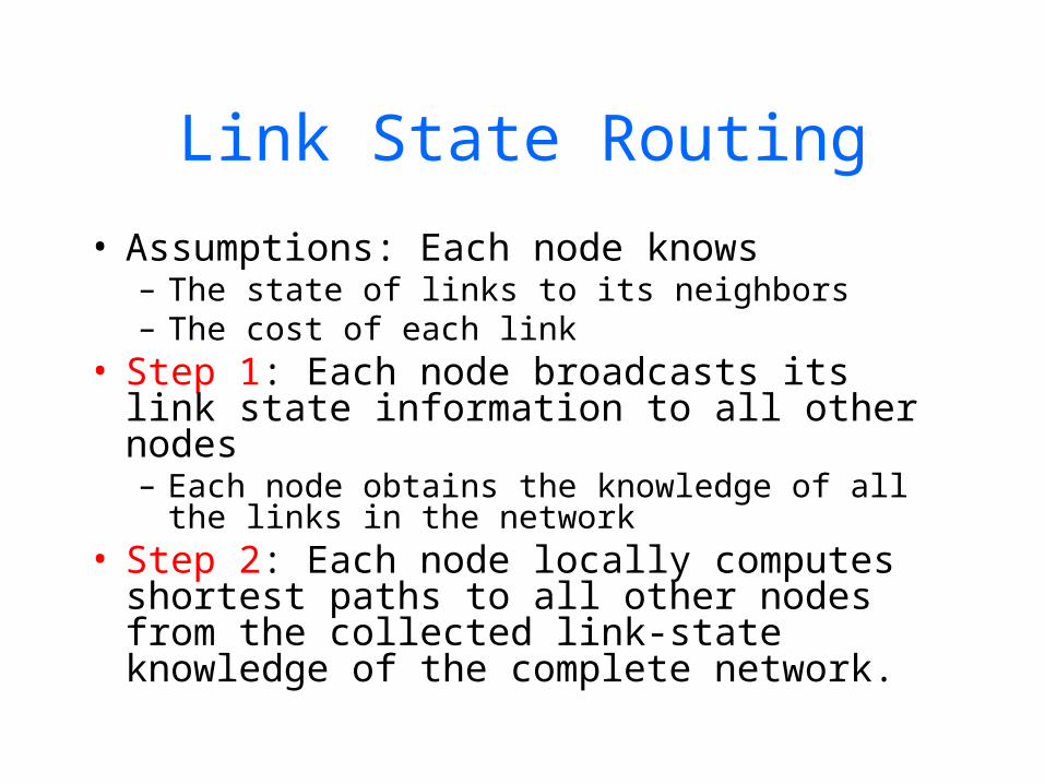
Link State Routing
• Assumptions: Each node knows – The state of links to its neighbors– The cost of each link
• Step 1: Each node broadcasts its link state information to all other nodes– Each node obtains the knowledge of all the
links in the network• Step 2: Each node locally computes
shortest paths to all other nodes from the collected link-state knowledge of the complete network.
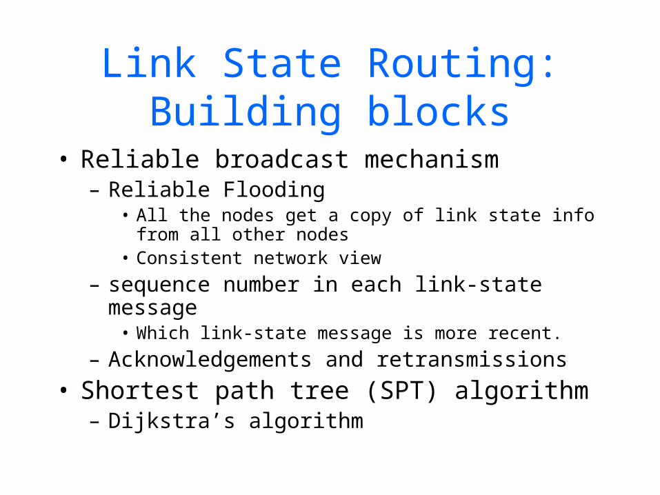
Link State Routing: Building blocks
• Reliable broadcast mechanism– Reliable Flooding
• All the nodes get a copy of link state info from all other nodes
• Consistent network view
– sequence number in each link-state message
• Which link-state message is more recent.
– Acknowledgements and retransmissions
• Shortest path tree (SPT) algorithm– Dijkstra’s algorithm
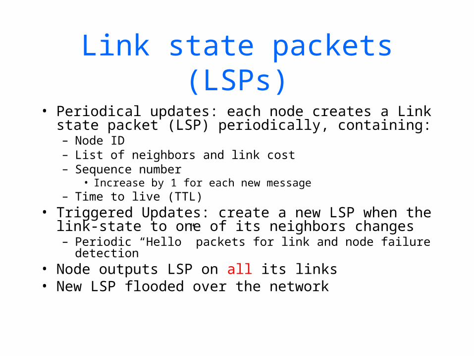
Link state packets (LSPs)
• Periodical updates: each node creates a Link state packet (LSP) periodically, containing:– Node ID– List of neighbors and link cost– Sequence number
• Increase by 1 for each new message– Time to live (TTL)
• Triggered Updates: create a new LSP when the link-state to one of its neighbors changes– Periodic “Hello” packets for link and node failure
detection• Node outputs LSP on all its links• New LSP flooded over the network
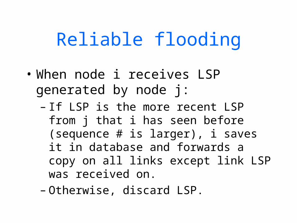
Reliable flooding
• When node i receives LSP generated by node j:– If LSP is the more recent LSP from j
that i has seen before (sequence # is larger), i saves it in database and forwards a copy on all links except link LSP was received on.
– Otherwise, discard LSP.
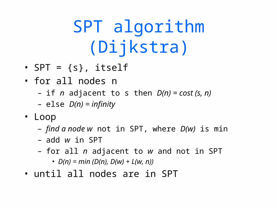
SPT algorithm (Dijkstra)
• SPT = {s}, itself• for all nodes n
– if n adjacent to s then D(n) = cost (s, n)– else D(n) = infinity
• Loop– find a node w not in SPT, where D(w) is min– add w in SPT– for all n adjacent to w and not in SPT
• D(n) = min (D(n), D(w) + L(w, n))
• until all nodes are in SPT
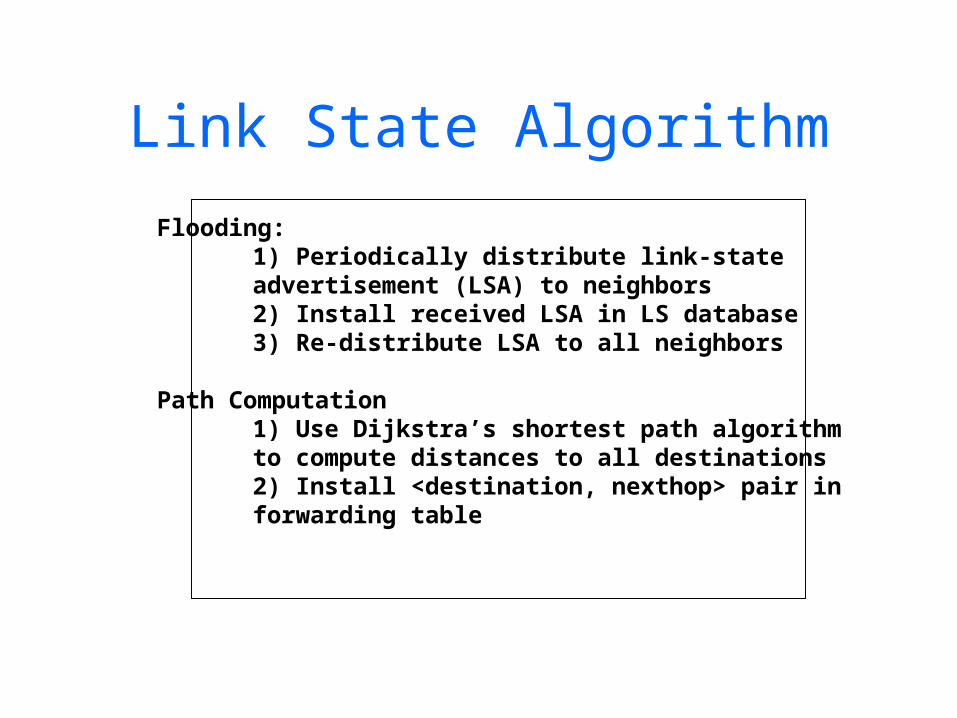
Link State Algorithm
Flooding:1) Periodically distribute link-state advertisement (LSA) to neighbors2) Install received LSA in LS database3) Re-distribute LSA to all neighbors
Path Computation1) Use Dijkstra’s shortest path algorithmto compute distances to all destinations2) Install <destination, nexthop> pair inforwarding table
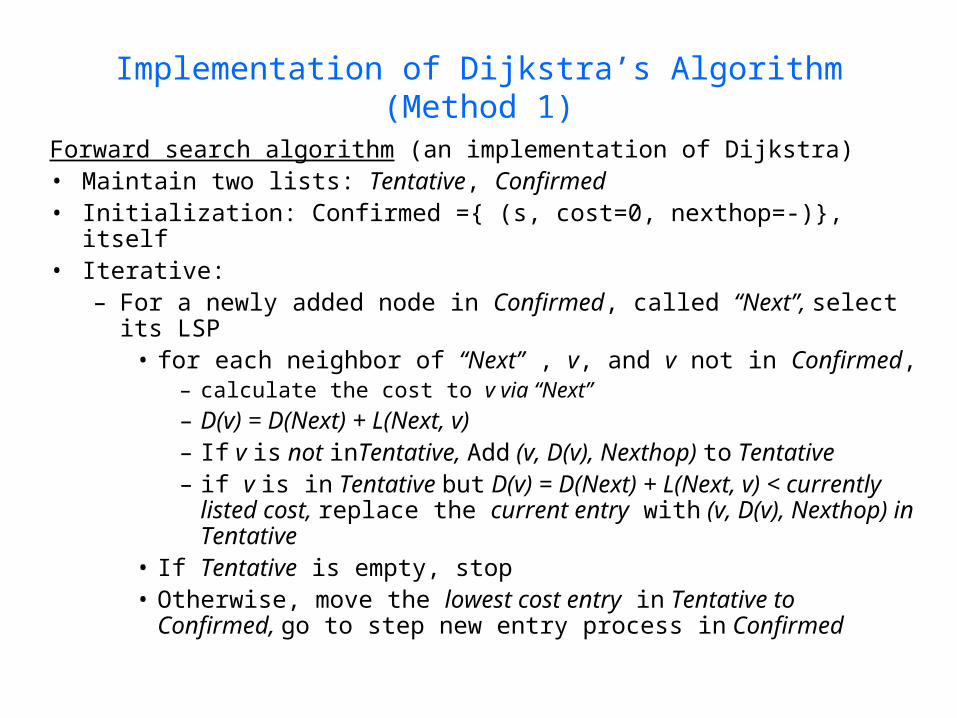
Implementation of Dijkstra’s Algorithm (Method 1)
Forward search algorithm (an implementation of Dijkstra)• Maintain two lists: Tentative, Confirmed• Initialization: Confirmed ={ (s, cost=0, nexthop=-)}, itself• Iterative:
– For a newly added node in Confirmed, called “Next”, select its LSP
• for each neighbor of “Next” , v, and v not in Confirmed, – calculate the cost to v via “Next”– D(v) = D(Next) + L(Next, v)– If v is not inTentative, Add (v, D(v), Nexthop) to
Tentative– if v is in Tentative but D(v) = D(Next) + L(Next, v) <
currently listed cost, replace the current entry with (v, D(v), Nexthop) in Tentative
• If Tentative is empty, stop• Otherwise, move the lowest cost entry in Tentative to
Confirmed, go to step new entry process in Confirmed
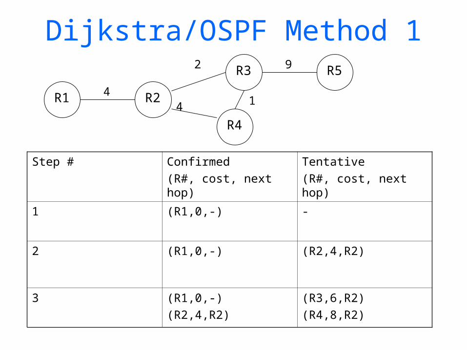
Dijkstra/OSPF Method 1
R1 R2
R4
R3 R5
4
2 9
4 1
Step # Confirmed(R#, cost, next hop)
Tentative(R#, cost, next hop)
1 (R1,0,-) -
2 (R1,0,-) (R2,4,R2)
3 (R1,0,-)(R2,4,R2)
(R3,6,R2)(R4,8,R2)
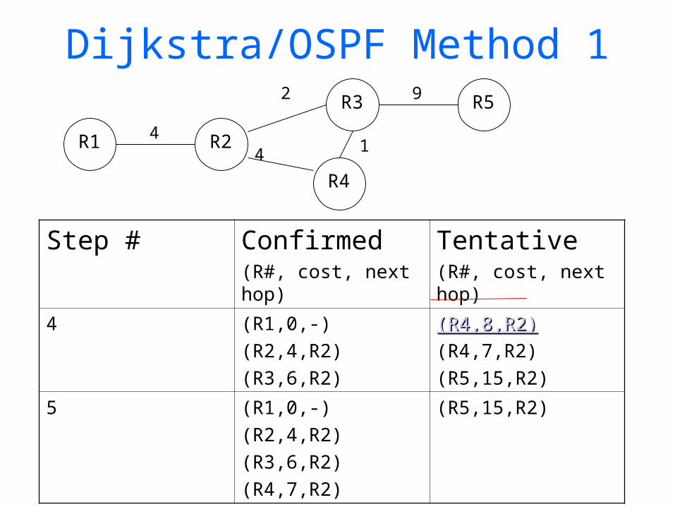
Dijkstra/OSPF Method 1
R1 R2
R4
R3 R5
4
2 9
4 1
Step # Confirmed(R#, cost, next hop)
Tentative(R#, cost, next hop)
4 (R1,0,-)(R2,4,R2)(R3,6,R2)
(R4,8,R2)(R4,8,R2)(R4,7,R2)(R5,15,R2)
5 (R1,0,-)(R2,4,R2)(R3,6,R2)(R4,7,R2)
(R5,15,R2)
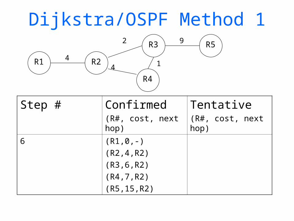
Dijkstra/OSPF Method 1
R1 R2
R4
R3 R5
4
2 9
4 1
Step # Confirmed(R#, cost, next hop)
Tentative(R#, cost, next hop)
6 (R1,0,-)(R2,4,R2)(R3,6,R2)(R4,7,R2)(R5,15,R2)
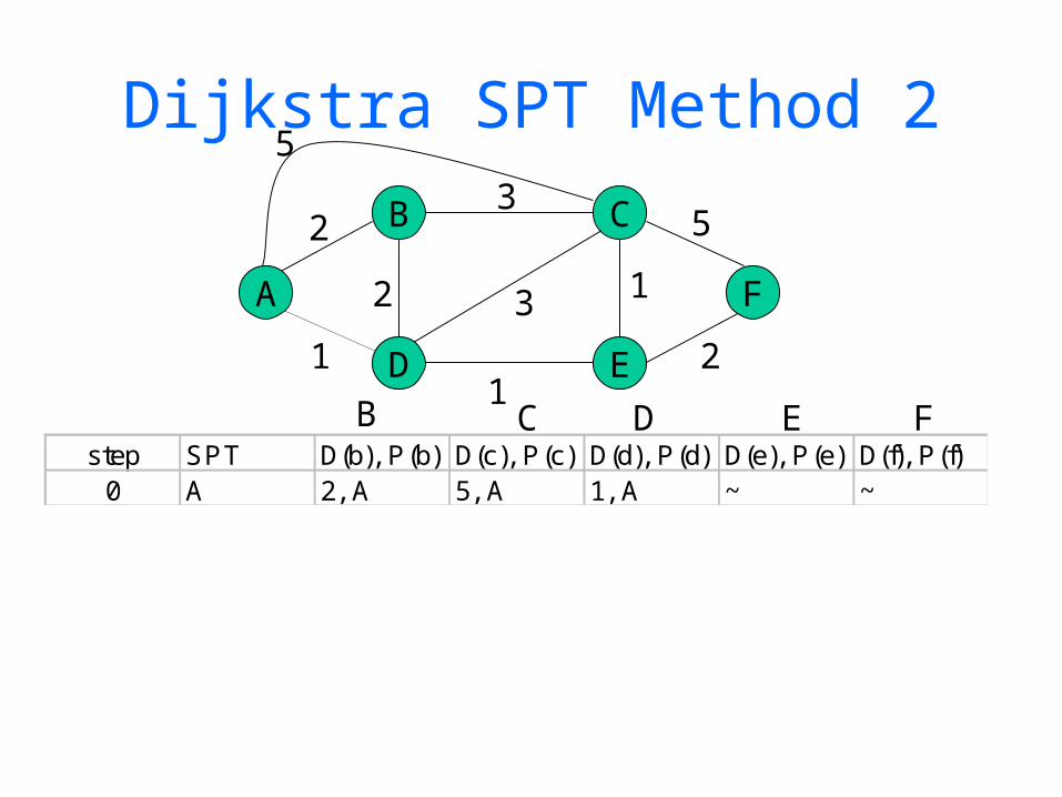
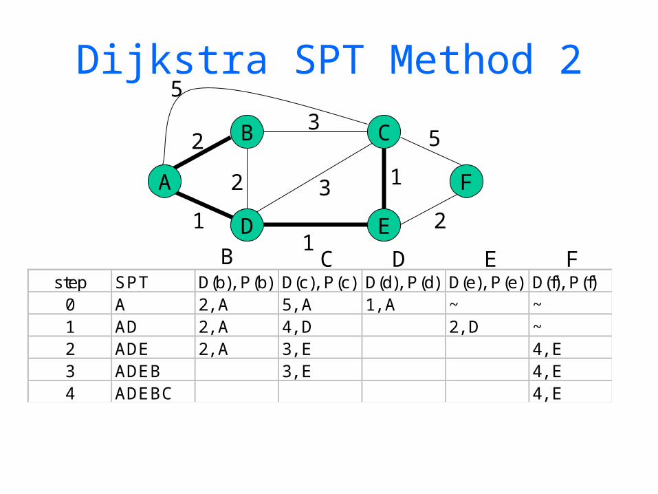
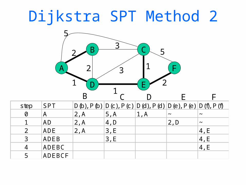
Dijkstra SPT Method 2
A F
B
D E
C2
2
2
3
1
1
1
3
5
step SPT D(b), P(b) D(c), P(c) D(d), P(d) D(e), P(e) D(f), P(f)0 A 2, A 5, A 1, A ~ ~
5
B C D E F
A F
B
D E
C2
2
2
3
1
1
1
3
5
step SPT D(b), P(b) D(c), P(c) D(d), P(d) D(e), P(e) D(f), P(f)0 A 2, A 5, A 1, A ~ ~1 AD 2, A 4, D 2, D ~
5
B C D E F
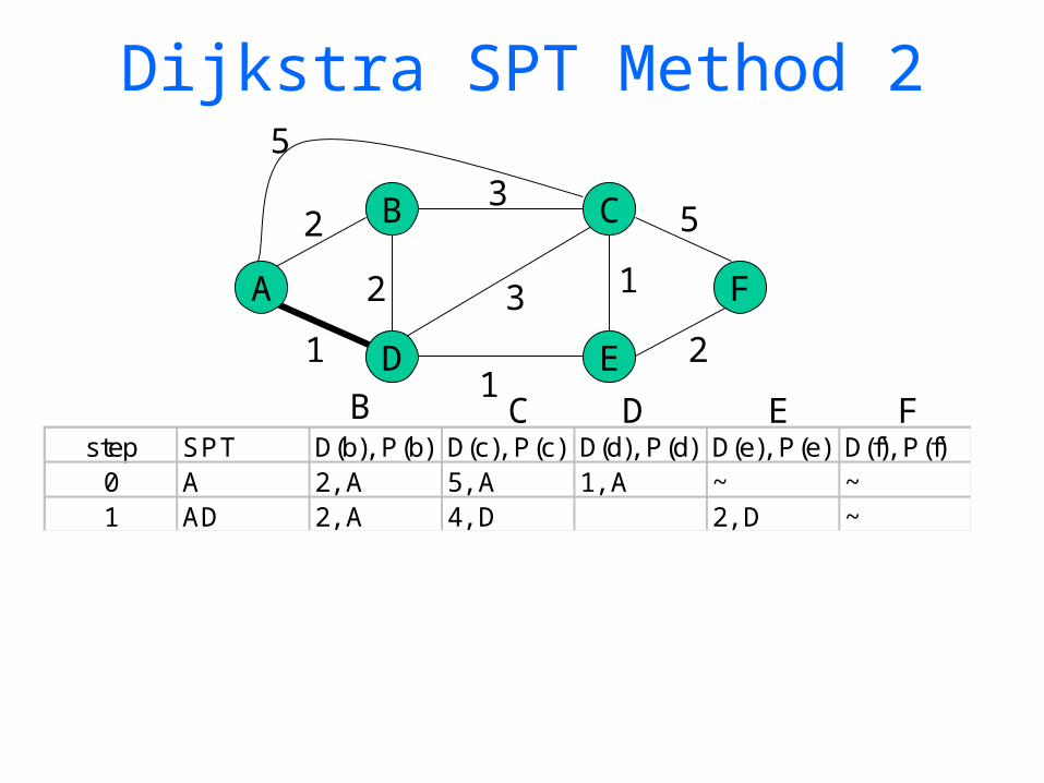
Dijkstra SPT Method 2
A F
B
D E
C2
2
2
3
1
1
1
3
5
step SPT D(b), P(b) D(c), P(c) D(d), P(d) D(e), P(e) D(f), P(f)0 A 2, A 5, A 1, A ~ ~1 AD 2, A 4, D 2, D ~2 ADE 2, A 3, E 4, E
5
B C D E F
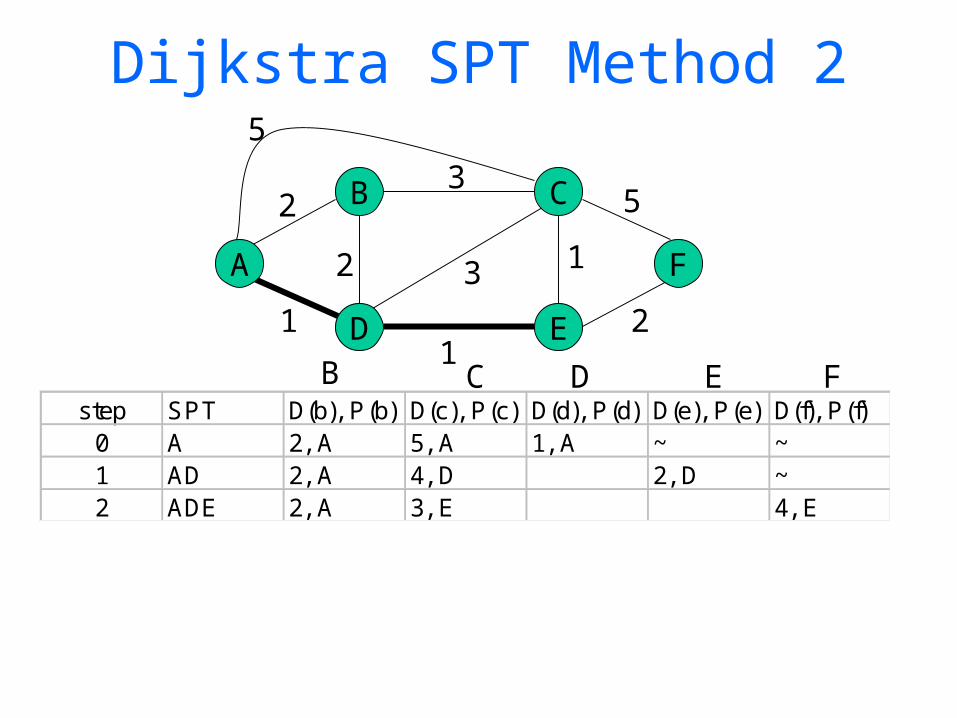
Dijkstra SPT Method 2
A F
B
D E
C2
2
2
3
1
1
1
3
5
step SPT D(b), P(b) D(c), P(c) D(d), P(d) D(e), P(e) D(f), P(f)0 A 2, A 5, A 1, A ~ ~1 AD 2, A 4, D 2, D ~2 ADE 2, A 3, E 4, E3 ADEB 3, E 4, E
5
B C D E F
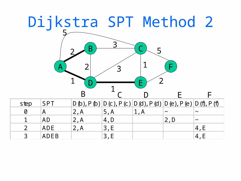
Dijkstra SPT Method 2
A F
B
D E
C2
2
2
3
1
1
1
3
5
step SPT D(b), P(b) D(c), P(c) D(d), P(d) D(e), P(e) D(f), P(f)0 A 2, A 5, A 1, A ~ ~1 AD 2, A 4, D 2, D ~2 ADE 2, A 3, E 4, E3 ADEB 3, E 4, E4 ADEBC 4, E
5
B C D E F
Dijkstra SPT Method 2
A F
B
D E
C2
2
2
3
1
1
1
3
5
step SPT D(b), P(b) D(c), P(c) D(d), P(d) D(e), P(e) D(f), P(f)0 A 2, A 5, A 1, A ~ ~1 AD 2, A 4, D 2, D ~2 ADE 2, A 3, E 4, E3 ADEB 3, E 4, E4 ADEBC 4, E5 ADEBCF
5
B C D E F
Dijkstra SPT Method 2
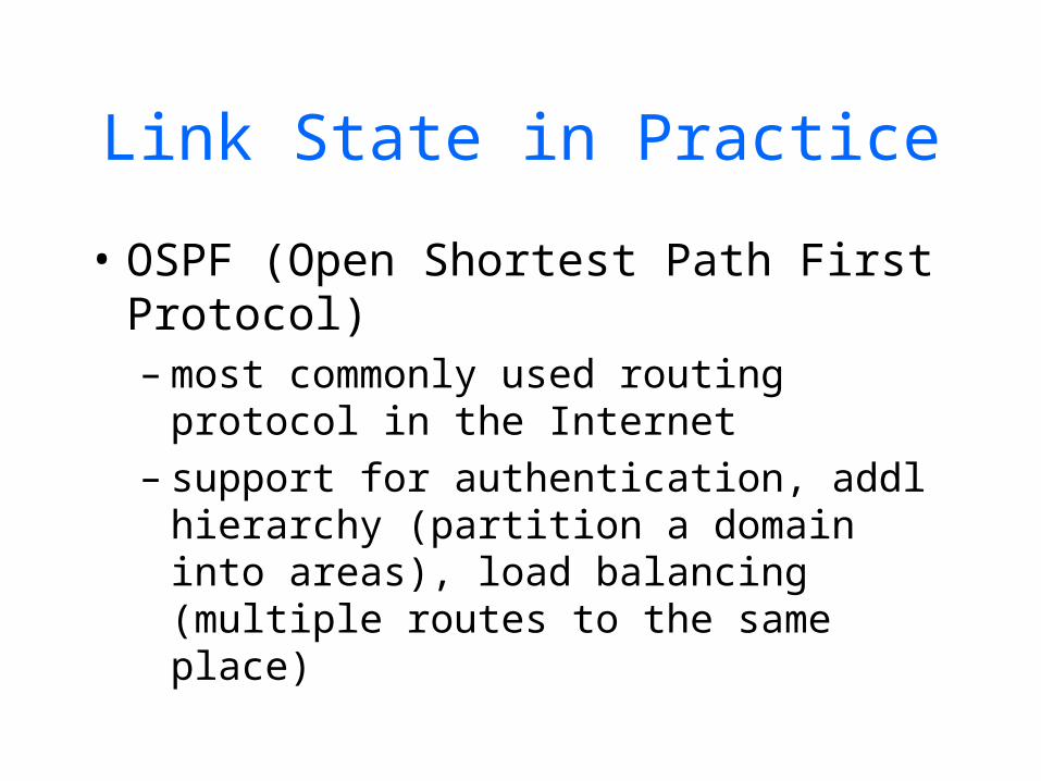
Link State in Practice
• OSPF (Open Shortest Path First Protocol)– most commonly used routing protocol
in the Internet– support for authentication, addl
hierarchy (partition a domain into areas), load balancing (multiple routes to the same place)
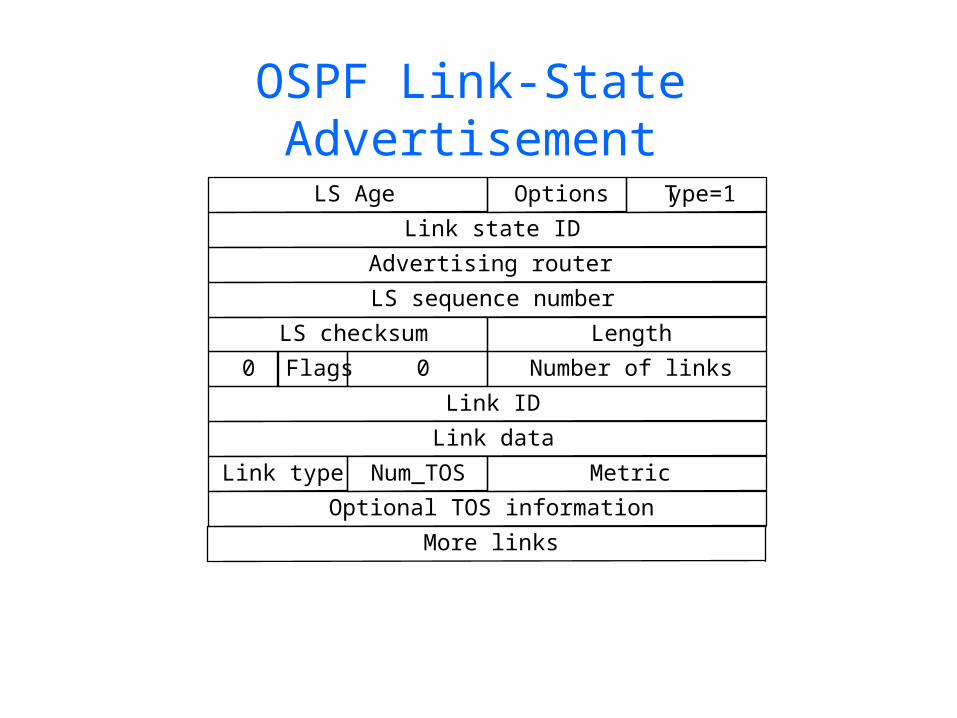
OSPF Link-State Advertisement
LS Age Options Type=1
0 Flags 0 Number of links
Link type Num_TOS Metric
Link state ID
Advertising router
LS sequence number
Link ID
Link data
Optional TOS information
More links
LS checksum Length
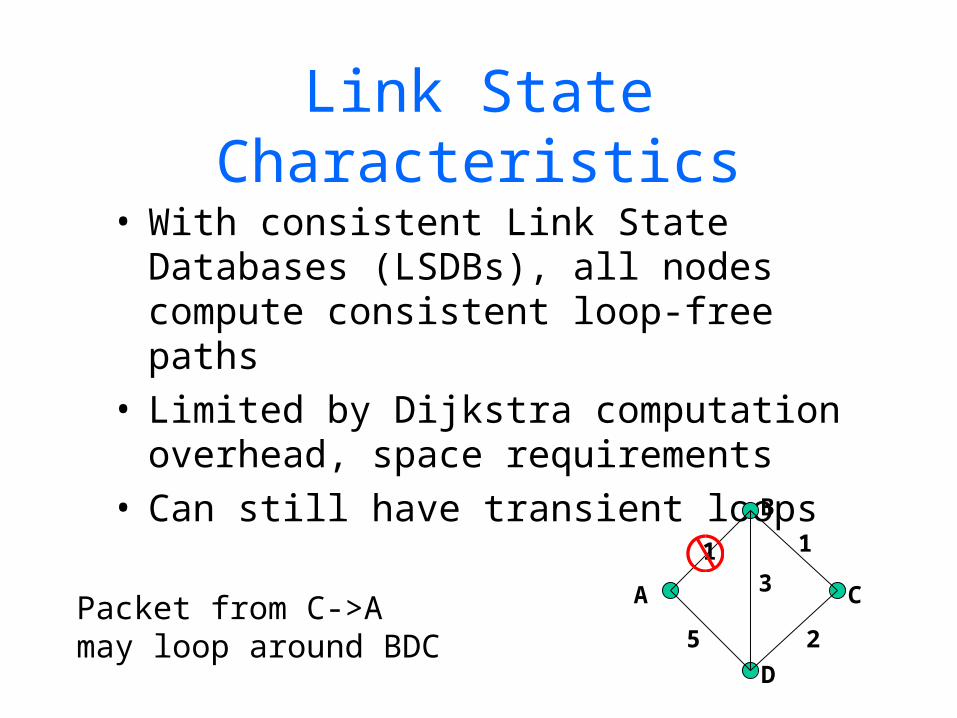
Link State Characteristics
• With consistent Link State Databases (LSDBs), all nodes compute consistent loop-free paths
• Limited by Dijkstra computation overhead, space requirements
• Can still have transient loops
A
B
C
D
13
5 2
1
Packet from C->Amay loop around BDC
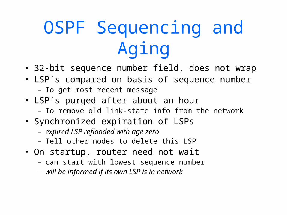
OSPF Sequencing and Aging
• 32-bit sequence number field, does not wrap• LSP’s compared on basis of sequence number
– To get most recent message
• LSP’s purged after about an hour– To remove old link-state info from the network
• Synchronized expiration of LSPs– expired LSP reflooded with age zero– Tell other nodes to delete this LSP
• On startup, router need not wait– can start with lowest sequence number– will be informed if its own LSP is in network
Problem: Router Failure
• A failed router and comes up but does not remember the last sequence number it used before it crashed
• New LSPs may be ignored if they have lower sequence number
One solution: LSP Aging
• Nodes periodically decrement age (TTL) of stored LSPs
• LSPs expire when TTL reaches 0– LSP is re-flooded once TTL = 0
• Rebooted router waits until all LSPs have expired
• Trade-off between frequency of LSPs periodic updates (overhead) and router wait after reboot
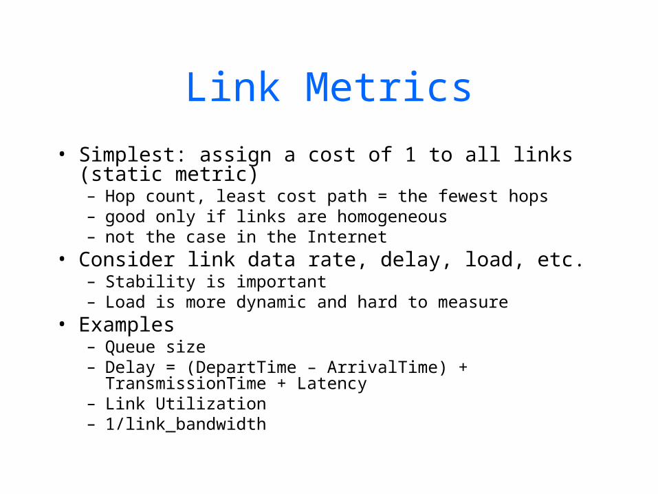
Link Metrics
• Simplest: assign a cost of 1 to all links (static metric)– Hop count, least cost path = the fewest hops– good only if links are homogeneous– not the case in the Internet
• Consider link data rate, delay, load, etc.– Stability is important– Load is more dynamic and hard to measure
• Examples– Queue size– Delay = (DepartTime – ArrivalTime) +
TransmissionTime + Latency– Link Utilization– 1/link_bandwidth
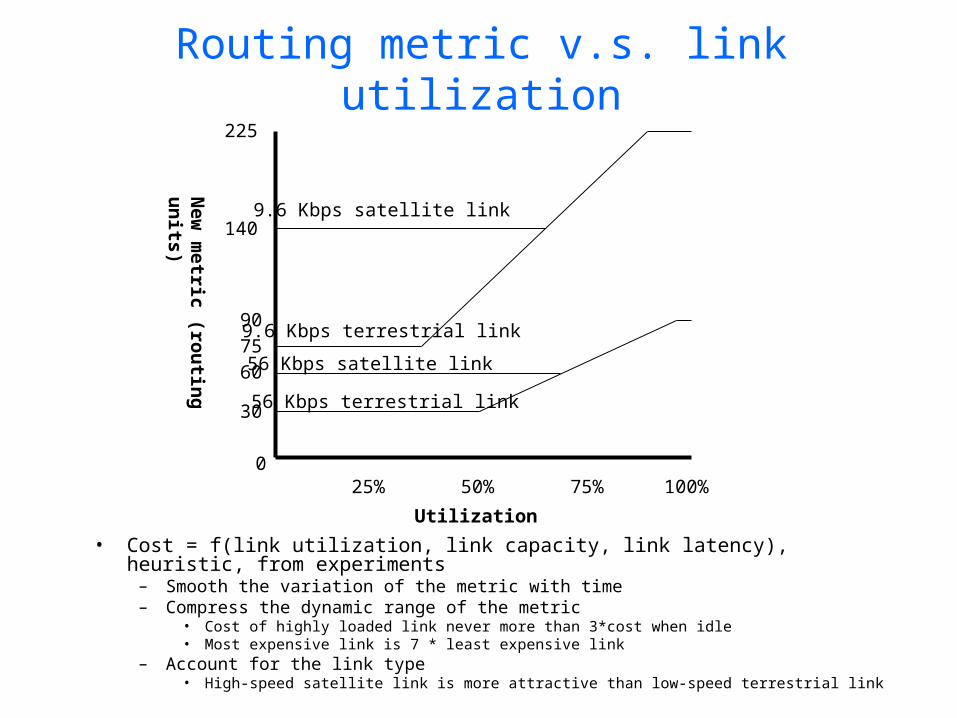
Routing metric v.s. link utilization
• Cost = f(link utilization, link capacity, link latency), heuristic, from experiments
– Smooth the variation of the metric with time– Compress the dynamic range of the metric
• Cost of highly loaded link never more than 3*cost when idle• Most expensive link is 7 * least expensive link
– Account for the link type• High-speed satellite link is more attractive than low-speed terrestrial link
0
30
60
140
75
50% 100%25% 75%
225
Utilization
9.6 Kbps satellite link
9.6 Kbps terrestrial link
56 Kbps terrestrial link
56 Kbps satellite link
90
New
metric (rou
ting u
nits)
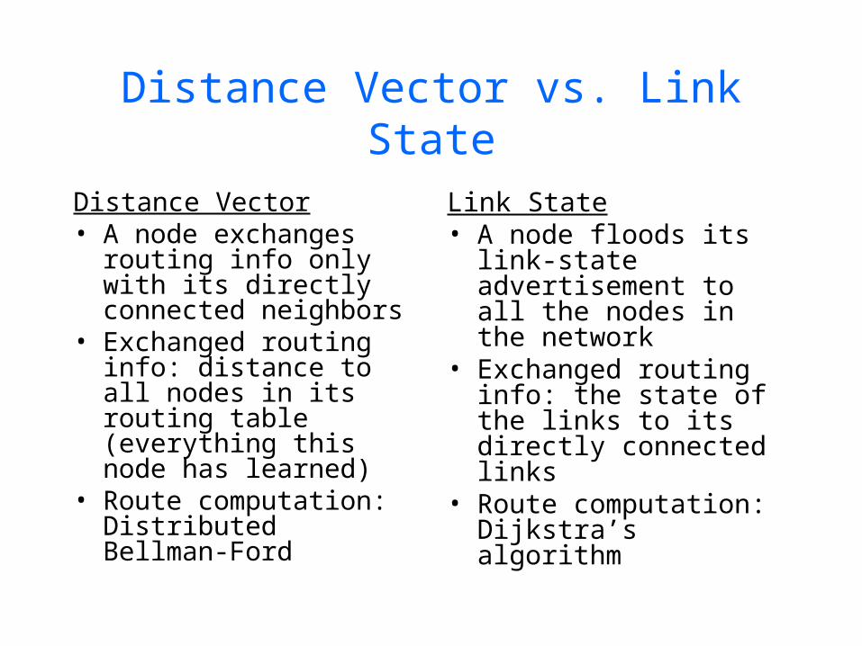
Distance Vector vs. Link State
Distance Vector• A node exchanges
routing info only with its directly connected neighbors
• Exchanged routing info: distance to all nodes in its routing table (everything this node has learned)
• Route computation: Distributed Bellman-Ford
Link State• A node floods its
link-state advertisement to all the nodes in the network
• Exchanged routing info: the state of the links to its directly connected links
• Route computation: Dijkstra’s algorithm
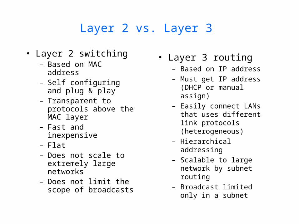
Layer 2 vs. Layer 3
• Layer 2 switching– Based on MAC
address– Self configuring and
plug & play– Transparent to
protocols above the MAC layer
– Fast and inexpensive
– Flat– Does not scale to
extremely large networks
– Does not limit the scope of broadcasts
• Layer 3 routing– Based on IP address– Must get IP address
(DHCP or manual assign)
– Easily connect LANs that uses different link protocols (heterogeneous)
– Hierarchical addressing– Scalable to large
network by subnet routing
– Broadcast limited only in a subnet
73
Today’s Homework• Peterson & Davie, Chap 4
-4.12-4.13-4.16-4.21Download and browse RIP and OSPF RFC’s
Due on Fri (2/27)