National Research Network S92

Industrial Geometry

http://www.industrial-geometry.at

Computer Aided Geometric Design

INDUSTRIAL

GEOMETRY

Computer Vision

NRN Report No. 99

Divide-and-conquer for Voronoidiagrams revisited

O. Aichholzer, W. Aigner, F. Aurenhammer,T. Hackl, B. Juttler, E. Pilgerstorfer, and

M. Rabl

January 2010

Divide-and-Conquer for Voronoi Diagrams Revisited✩

Oswin Aichholzer∗,a, Wolfgang Aignera, Franz Aurenhammerb, Thomas Hackla, Bert Juttlerc,Elisabeth Pilgerstorferc, Margot Rablc

aInstitute for Software Technology, Graz University of Technology, AustriabInstitute for Theoretical Computer Science, Graz University of Technology, Austria

cInstitute of Applied Geometry, Johannes Kepler UniversityLinz, Austria

Abstract

We show how to divide the edge graph of a Voronoi diagram into atree that corresponds to the medial axis of an(augmented) planar domain. Division into base cases is thenpossible, which, in the bottom-up phase, can be mergedby trivial concatenation. The resulting construction algorithm—similar to Delaunay triangulation methods—is notbisector-based and merely computes dual links between the sites, its atomic steps being inclusion tests for sites incircles. This guarantees computational simplicity and numerical stability. Moreover, no part of the Voronoi diagram,once constructed, has to be discarded again. The algorithm works for polygonal and curved objects as sites and, inparticular, for circular arcs, which allows its extension to general free-form objects by Voronoi diagram preservingand data saving biarc approximations. The algorithm is randomized, with expected runtimeO(n logn) under certainassumptions on the input data. Experiments substantiate anefficient behavior even when these assumptions are notmet. Applications to offset computations and motion planning for general objects are described.

Key words: Voronoi diagram, medial axis, divide-and-conquer, biarc approximation, trimmed offset, motionplanning

1. Introduction

The divide-and-conquer paradigm gave the first optimal solution for constructing the closest-site Voronoi diagramin the plane [28]. Though being a classical example for applying a powerful algorithmic method in computationalgeometry, the resulting algorithm became no favorite for implementation, not even in the case of point sites.

For Voronoi diagrams of general objects the situation is more intricate, as such diagrams may have all kinds ofartifacts. Their edge graph may be disconnected, and their bisectors may be closed curves, which complicates theconstruction. In particular, the abstract Voronoi diagrammachinery in [18, 19] is ruled out. Literature tells us thatdivide-and-conquer is involved if emphasis is on the bottom-up phase, even if the sites are of relatively simple shape.See the papers [22] and [29], respectively, for early algorithms on line segments and circles, and the optimalO(n logn)variants in [17] for line segments, in [31] for line segmentsand circular arcs, and in [7] for convex distance functions.The crux is the missing separability condition for the sites, which would prevent the merge curve from breaking intoseveral components. Even this issue being solved, we still have to intersect complicated bisectors and discard oldparts of the diagram, which makes the algorithms complex andhard to implement.

Many alternative strategies for computing generalized Voronoi diagrams have been tried. Incremental insertioncannot be applied directly to general sites without loss of efficiency. In particular, the framework in [19] for abstract

✩Supported by the Austrian FWF Joint Research Project ’Industrial Geometry’, S9202-N12 and S9205-N12.∗corresponding authorEmail addresses:oaich@ist.tugraz.at (Oswin Aichholzer),waigner@ist.tugraz.at (Wolfgang Aigner),auren@igi.tugraz.at

(Franz Aurenhammer),thackl@ist.tugraz.at (Thomas Hackl),Bert.Juettler@jku.at (Bert Juttler),Elisabeth.Pilgerstorfer@jku.at (Elisabeth Pilgerstorfer),Margot.Rabl@jku.at (Margot Rabl)

Preprint submitted to Computational Geometry - Theory and Applications December 15, 2009

(a) Point sites (b) Mixed sites

Figure 1: Voronoi diagrams for different kinds of sites.

Voronoi diagrams may not apply. Still, randomized insertion can be made efficient [3], but needs pre-requisites likesplitting sites into ’harmless’ pieces, each piece then acting as several sites. The plane-sweep technique, on the otherhand, generalizes nicely for line segments and circles [12]but, unfortunately, not for circular arcs or more generalsites. Line segments have to be split into 3 sites to ‘domesticate’ their bisector. Many implementation details occur.

In fact, in all these algorithms the bisector curves take part in the computation. Already in the case of linesegments, bisectors are composed of up to 7 pieces, and may even be two-dimensional if not defined carefully in thecase of shared endpoints. Such situations cannot be considered degenerate; they occur naturally when decomposingcomplex sites into simpler ones. Consequently, the algorithms are involved and also suffer from numerical imprecison.Difficulties may be partially eluded when working in the dual environment: Instead of intersecting two bisectors, thecenter of a circle tangent to the three defining sites is calculated. This bears the advantage of working on the sitesdirectly, linking them accordingly rather than computing new geometric objects that themselves take part in latercalculations. The classical example is, of course, the Delaunay triangulation for point sites. For general sites, tangentcircles may not be unique. Up to 8 solutions do exist, which are usually difficult to calculate; see e.g. [11].

The algorithm we propose in the present paper works directlyon the sites, too, but its atomic operation is muchsimpler, namely, an inclusion test of a site in afixedcircle. We first extract the combinatorial structure of the Voronoidiagram, and fill in the bisector curves later on. In contrastto existing Voronoi/Delaunay algorithms, no constructedobject is ever discarded. Our setting is very general: Sitesare pairwise disjoint topological disks of dimensionstwo, one, or zero. This includes polygonal sites, circular disks, spline curves, but also single points and straight-linesegments. Boundaries of curved planar objects with holes can be modeled. We do not split complex sites into piecesbeforehand, because we need not care about the bisectors.

Our idea is to calibrate the top-down phase of divide-and-conquer by dividing the edge graph of the Voronoidiagram without prior knowledge. A simple plane sweep is used to generate a set of points whose removal from theedge graph leaves a geometric tree. This tree is then computable as the medial axis of a generalized domain that,combinatorially, behaves like a simply connected domain. While classical medial axis algorithms [21, 6, 8] cannot beapplied, not even in the presence of simple sites, we show that the methods in [2, 1] are flexible enough to be extendedto work for such domains. In particular, the edge graph is split further in a recursive manner, until directly solvablebase cases remain. The bottom-up phase is trivial and consists of reassembling the respective pieces of the edge graph.

The paper includes a theoretical and an applied part. We takeparticular interest in sites represented by circular arcsplines, for several reasons. The modeling power of such splines beats that of polylines, which results in a significantlysmaller input data volume. Our algorithm naturally, and with almost no increase of numeric complexity, works for thiscase. Also, a stable approximation of the Voronoi diagram for algebraically complex original sites can be guaranteed.

2

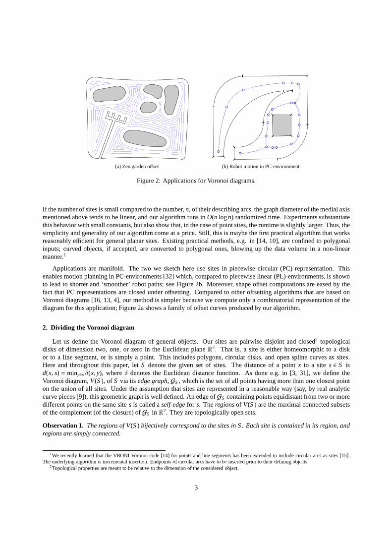
(a) Zen garden offset (b) Robot motion in PC-environment

Figure 2: Applications for Voronoi diagrams.

If the number of sites is small compared to the number,n, of their describing arcs, the graph diameter of the medial axismentioned above tends to be linear, and our algorithm runs inO(n logn) randomized time. Experiments substantiatethis behavior with small constants, but also show that, in the case of point sites, the runtime is slightly larger. Thus, thesimplicity and generality of our algorithm come at a price. Still, this is maybe the first practical algorithm that worksreasonably efficient for general planar sites. Existing practical methods, e.g. in [14, 10], are confined to polygonalinputs; curved objects, if accepted, are converted to polygonal ones, blowing up the data volume in a non-linearmanner.1

Applications are manifold. The two we sketch here use sites in piecewise circular (PC) representation. Thisenables motion planning in PC-environments [32] which, compared to piecewise linear (PL)-environments, is shownto lead to shorter and ‘smoother’ robot paths; see Figure 2b.Moreover, shape offset computations are eased by thefact that PC representations are closed under offsetting. Compared to other offsetting algorithms that are based onVoronoi diagrams [16, 13, 4], our method is simpler because we compute only a combinatorial representation of thediagram for this application; Figure 2a shows a family of offset curves produced by our algorithm.

2. Dividing the Voronoi diagram

Let us define the Voronoi diagram of general objects. Our sites are pairwise disjoint and closed2 topologicaldisks of dimension two, one, or zero in the Euclidean planeR

2. That is, a site is either homeomorphic to a diskor to a line segment, or is simply a point. This includes polygons, circular disks, and open spline curves as sites.Here and throughout this paper, letS denote the given set of sites. The distance of a pointx to a sites ∈ S isd(x, s) = miny∈s δ(x, y), whereδ denotes the Euclidean distance function. As done e.g. in [3,31], we define theVoronoi diagram,V(S), of S via its edge graph,GS, which is the set of all points having more than one closest pointon the union of all sites. Under the assumption that sites arerepresented in a reasonable way (say, by real analyticcurve pieces [9]), this geometric graph is well defined. An edge ofGS containing points equidistant from two or moredifferent points on the same sites is called aself-edgefor s. Theregionsof V(S) are the maximal connected subsetsof the complement (of the closure) ofGS in R

2. They are topologically open sets.

Observation 1. The regions of V(S) bijectively correspond to the sites in S . Each site is contained in its region, andregions are simply connected.

1We recently learned that the VRONI Voronoi code [14] for points and line segments has been extended to include circular arcs as sites [15].The underlying algorithm is incremental insertion. Endpoints of circular arcs have to be inserted prior to their defining objects.

2Topological properties are meant to be relative to the dimension of the considered object.

3

Au

v

A0

D1

D2

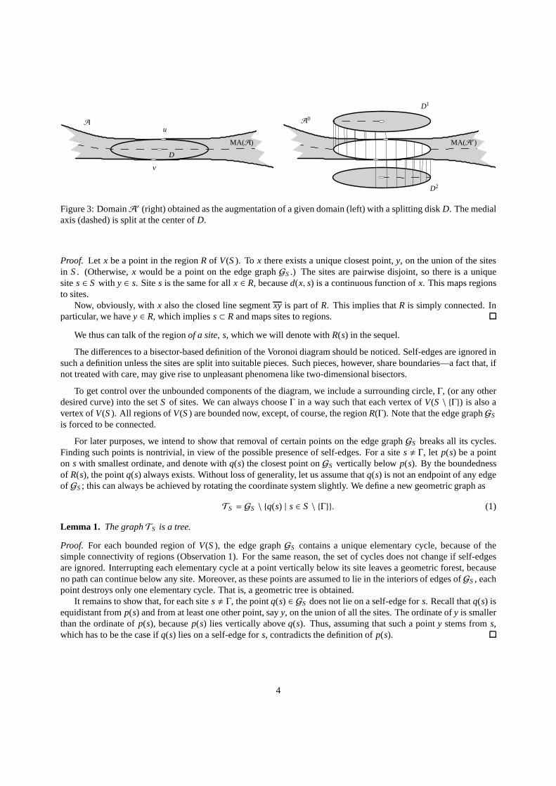
MA(A) MA(A′)D

Figure 3: DomainA′ (right) obtained as the augmentation of a given domain (left) with a splitting diskD. The medialaxis (dashed) is split at the center ofD.

Proof. Let x be a point in the regionR of V(S). To x there exists a unique closest point,y, on the union of the sitesin S. (Otherwise,x would be a point on the edge graphGS.) The sites are pairwise disjoint, so there is a uniquesites ∈ S with y ∈ s. Sites is the same for allx ∈ R, becaused(x, s) is a continuous function ofx. This maps regionsto sites.

Now, obviously, withx also the closed line segmentxy is part ofR. This implies thatR is simply connected. Inparticular, we havey ∈ R, which impliess⊂ R and maps sites to regions.

We thus can talk of the regionof a site, s, which we will denote withR(s) in the sequel.

The differences to a bisector-based definition of the Voronoi diagram should be noticed. Self-edges are ignored insuch a definition unless the sites are split into suitable pieces. Such pieces, however, share boundaries—a fact that, ifnot treated with care, may give rise to unpleasant phenomenalike two-dimensional bisectors.

To get control over the unbounded components of the diagram,we include a surrounding circle,Γ, (or any otherdesired curve) into the setS of sites. We can always chooseΓ in a way such that each vertex ofV(S \ {Γ}) is also avertex ofV(S). All regions ofV(S) are bounded now, except, of course, the regionR(Γ). Note that the edge graphGS

is forced to be connected.

For later purposes, we intend to show that removal of certainpoints on the edge graphGS breaks all its cycles.Finding such points is nontrivial, in view of the possible presence of self-edges. For a sites, Γ, let p(s) be a pointon s with smallest ordinate, and denote withq(s) the closest point onGS vertically belowp(s). By the boundednessof R(s), the pointq(s) always exists. Without loss of generality, let us assume that q(s) is not an endpoint of any edgeof GS; this can always be achieved by rotating the coordinate system slightly. We define a new geometric graph as

TS = GS \ {q(s) | s ∈ S \ {Γ}}. (1)

Lemma 1. The graphTS is a tree.

Proof. For each bounded region ofV(S), the edge graphGS contains a unique elementary cycle, because of thesimple connectivity of regions (Observation 1). For the same reason, the set of cycles does not change if self-edgesare ignored. Interrupting each elementary cycle at a point vertically below its site leaves a geometric forest, becauseno path can continue below any site. Moreover, as these points are assumed to lie in the interiors of edges ofGS, eachpoint destroys only one elementary cycle. That is, a geometric tree is obtained.

It remains to show that, for each sites, Γ, the pointq(s) ∈ GS does not lie on a self-edge fors. Recall thatq(s) isequidistant fromp(s) and from at least one other point, sayy, on the union of all the sites. The ordinate ofy is smallerthan the ordinate ofp(s), becausep(s) lies vertically aboveq(s). Thus, assuming that such a pointy stems froms,which has to be the case ifq(s) lies on a self-edge fors, contradicts the definition ofp(s).

4

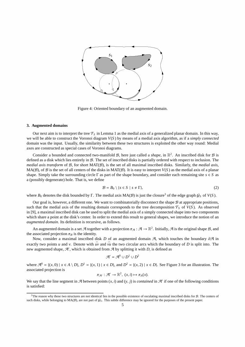
s1

s2

Figure 4: Oriented boundary of an augmented domain.

3. Augmented domains

Our next aim is to interpret the treeTS in Lemma 1 as the medial axis of a generalized planar domain. In this way,we will be able to construct the Voronoi diagramV(S) by means of a medial axis algorithm, as if asimply connecteddomain was the input. Usually, the similarity between thesetwo structures is exploited the other way round: Medialaxes are constructed as special cases of Voronoi diagrams.

Consider a bounded and connected two-manifoldB, here just called ashape, in R2. An inscribed disk forB is

defined as a disk which lies entirely inB. The set of inscribed disks is partially ordered with respect to inclusion. Themedial axis transformof B, for short MAT(B), is the set of all maximal inscribed disks. Similarly, themedial axis,MA(B), ofB is the set of all centers of the disks in MAT(B). It is easy to interpretV(S) as the medial axis of a planarshape. Simply take the surrounding circleΓ as part of the shape boundary, and consider each remaining site s ∈ S asa (possibly degenerate) hole. That is, we define

B = B0 \ {s ∈ S | s, Γ}, (2)

whereB0 denotes the disk bounded byΓ. The medial axis MA(B) is just the closure3 of the edge graphGS of V(S).

Our goal is, however, a different one. We want to combinatorially disconnect the shapeB at appropriate positions,such that the medial axis of the resulting domain corresponds to the tree decompositionTS of V(S). As observedin [9], a maximal inscribed disk can be used to split the medial axis of a simply connected shape into two componentswhich share a point at the disk’s center. In order to extend this result to general shapes, we introduce the notion of anaugmented domain. Its definition is recursive, as follows.

An augmented domain is a setA together with a projectionπA : A → R2. Initially, A is the original shapeB, and

the associated projectionπB is the identity.Now, consider a maximal inscribed diskD of an augmented domainA, which touches the boundary∂A in

exactly two pointsu andv. Denote with⌣uv and

⌣vu the two circular arcs which the boundary ofD is split into. The

new augmented shape,A′, which is obtained fromA by splitting it with D, is defined as

A′ = A0 ∪ D1 ∪ D2

whereA0 = {(x, 0) | x ∈ A \ D}, D1 = {(x, 1) | x ∈ D}, andD2 = {(x, 2) | x ∈ D}. See Figure 3 for an illustration. Theassociated projection is

πA′ : A′ → R2, (x, i) 7→ πA(x).

We say that the line segment inA between points (x, i) and (y, j) is containedinA′ if one of the following conditionsis satisfied:

3The reason why these two structures are not identical lies inthe possible existence of osculating maximal inscribed disks forB. The centers ofsuch disks, while belonging to MA(B), are not part ofGS. This subtle difference may be ignored for the purposes of the present paper.

5

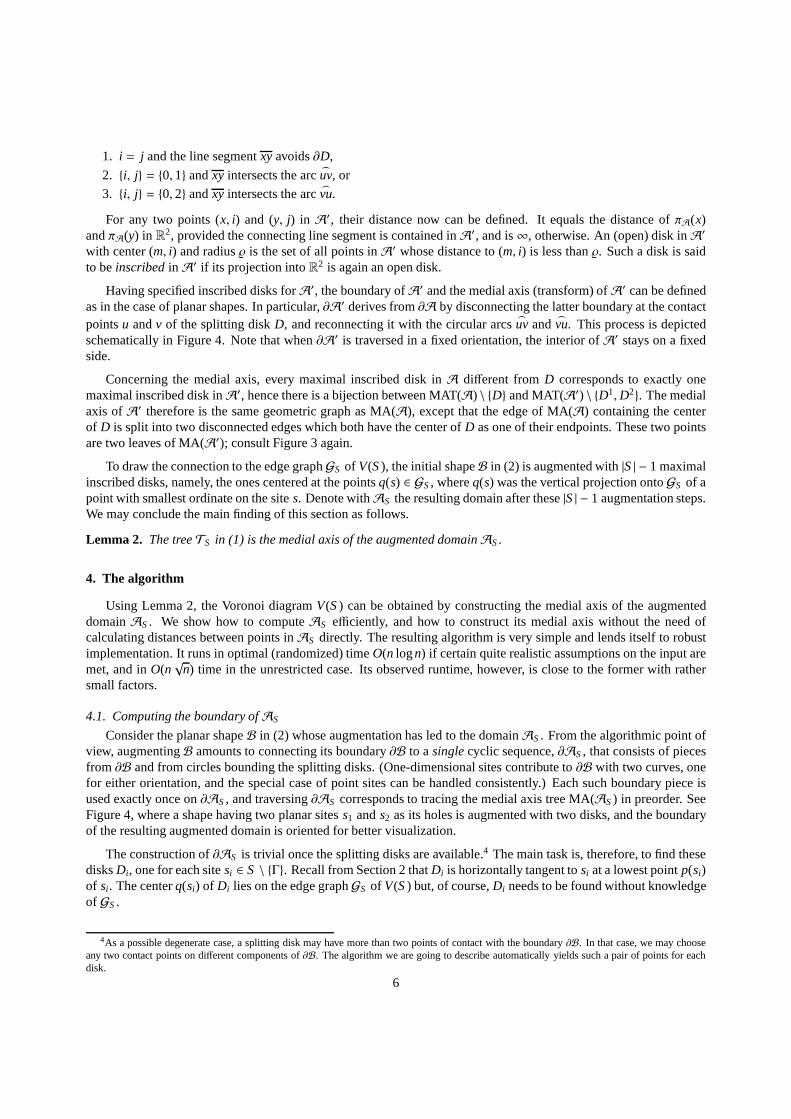
1. i = j and the line segmentxy avoids∂D,

2. {i, j} = {0, 1} andxy intersects the arc⌣uv, or

3. {i, j} = {0, 2} andxy intersects the arc⌣vu.

For any two points (x, i) and (y, j) in A′, their distance now can be defined. It equals the distance ofπA(x)andπA(y) in R

2, provided the connecting line segment is contained inA′, and is∞, otherwise. An (open) disk inA′with center (m, i) and radius is the set of all points inA′ whose distance to (m, i) is less than . Such a disk is saidto beinscribedinA′ if its projection intoR

2 is again an open disk.

Having specified inscribed disks forA′, the boundary ofA′ and the medial axis (transform) ofA′ can be definedas in the case of planar shapes. In particular,∂A′ derives from∂A by disconnecting the latter boundary at the contactpointsu andv of the splitting diskD, and reconnecting it with the circular arcs

⌣uv and

⌣vu. This process is depicted

schematically in Figure 4. Note that when∂A′ is traversed in a fixed orientation, the interior ofA′ stays on a fixedside.

Concerning the medial axis, every maximal inscribed disk inA different fromD corresponds to exactly onemaximal inscribed disk inA′, hence there is a bijection between MAT(A) \ {D} and MAT(A′) \ {D1,D2}. The medialaxis ofA′ therefore is the same geometric graph as MA(A), except that the edge of MA(A) containing the centerof D is split into two disconnected edges which both have the center of D as one of their endpoints. These two pointsare two leaves of MA(A′); consult Figure 3 again.

To draw the connection to the edge graphGS of V(S), the initial shapeB in (2) is augmented with|S| − 1 maximalinscribed disks, namely, the ones centered at the pointsq(s) ∈ GS, whereq(s) was the vertical projection ontoGS of apoint with smallest ordinate on the sites. Denote withAS the resulting domain after these|S| − 1 augmentation steps.We may conclude the main finding of this section as follows.

Lemma 2. The treeTS in (1) is the medial axis of the augmented domainAS.

4. The algorithm

Using Lemma 2, the Voronoi diagramV(S) can be obtained by constructing the medial axis of the augmenteddomainAS. We show how to computeAS efficiently, and how to construct its medial axis without the need ofcalculating distances between points inAS directly. The resulting algorithm is very simple and lends itself to robustimplementation. It runs in optimal (randomized) timeO(n logn) if certain quite realistic assumptions on the input aremet, and inO(n

√n) time in the unrestricted case. Its observed runtime, however, is close to the former with rather

small factors.

4.1. Computing the boundary ofAS

Consider the planar shapeB in (2) whose augmentation has led to the domainAS. From the algorithmic point ofview, augmentingB amounts to connecting its boundary∂B to asinglecyclic sequence,∂AS, that consists of piecesfrom ∂B and from circles bounding the splitting disks. (One-dimensional sites contribute to∂B with two curves, onefor either orientation, and the special case of point sites can be handled consistently.) Each such boundary piece isused exactly once on∂AS, and traversing∂AS corresponds to tracing the medial axis tree MA(AS) in preorder. SeeFigure 4, where a shape having two planar sitess1 ands2 as its holes is augmented with two disks, and the boundaryof the resulting augmented domain is oriented for better visualization.

The construction of∂AS is trivial once the splitting disks are available.4 The main task is, therefore, to find thesedisksDi , one for each sitesi ∈ S \ {Γ}. Recall from Section 2 thatDi is horizontally tangent tosi at a lowest pointp(si)of si . The centerq(si) of Di lies on the edge graphGS of V(S) but, of course,Di needs to be found without knowledgeof GS.

4As a possible degenerate case, a splitting disk may have morethan two points of contact with the boundary∂B. In that case, we may chooseany two contact points on different components of∂B. The algorithm we are going to describe automatically yields such a pair of points for eachdisk.

6

Indeed, a simple and efficient plane-sweep can be applied as follows. Sweep acrossS from above to below witha horizontal lineL. For a sitesi , Γ, let xi be the abscissa ofp(si), and defineEL(i) = si ∩ L. Note thatEL(i) mayconsist of more than one component. We maintain, for each site si whose pointp(si) has been swept over, the sitesj

whereEL( j) is closest toxi onL. The unique disk with north polep(si) and touchingsj is computed, and the minimalsuch disk forsi so far,DL(i), is updated if necessary. The abscissaxi is deactivated again whenDL(i) has been fullyswept over byL.

Lemma 3. After completion of the sweep, DL(i) = Di holds for each index i.

Proof. For a fixed indexi, let sk be the site that defines the diskDi . We have to show thatEL(k) and xi becomeneighbors onL while xi is active. Consider a pointt whereDi is tangent tosk. Then, becauseDi avoids all the sites,the line segmentxi t ⊂ Di does the same. ThusEL(k) andxi are adjacent whenL passes throught. Also, xi is active atthis moment, becauseDi ⊂ DL(i) holds.

To keep small the number of neighbor pairs (xi , sj) on L processed during the plane sweep, we only consider pairswhere no other active abscissaxm lies betweenxi andEL( j); the diskDL(i) cannot have a contact beyond the oneof DL(m), otherwise. The number of such pairs is linear. Thus the construction can be implemented inO(n logn) timeif the sites inS are described by a total ofn objects, each being managable in constant time. Note that∂AS thenconsists ofΘ(n) pieces.

4.2. Computing the medial axis ofAS

Given the description of an augmented domain by its boundary, it may, at first glance, seem complicated tocompute its medial axis. In our case, however, the domainAS has a connected boundary. Therefore it can be splitinto subdomains with the same property using maximal inscribed disks. This suggests a divide-and-conquer algorithmfor computing MA(AS). The domain and its medial axis tree are split recursively,until directly solvable base casesremain. For simply connected shapes, a similar approach hasbeen applied in [2, 1].

In fact, it is easy to obtain splitting disks forAS. Recall that∂AS consists of pieces that bound inscribed disks(calledartificial arcs) and pieces that stem from site boundaries (calledsite segments). Now, to calculate a splittingdisk, the algorithm fixes some pointp on a site segment and computes a maximal inscribed diskD for AS thattouches∂AS at p. Starting with an (appropriately oriented) disk of large radius, ∂AS is scanned and the disk isshrunk accordingly whenever an intersection with a site segment occurs. Intersections with artificial arcs are, however,ignored.

Lemma 4. The algorithm above correctly computes the required disk D forAS at point p.

Proof. From Section 3 we know that the set of maximal inscribed disksis the same forAS and forB, except for the(finitely many) disks taking part in the augmentation. The assertion follows.

In other words, the distances to the sites which are needed inthe medial axis computation are the same inAS andin B. (This is, of course, not true forall possible distances.) Note that the artificial arcs are used only to link the sitesegments in the correct cyclic order; they do not play any geometric role. Computing a splitting disk takesO(n) time,if each object describing the sites can be handled inO(1) time.

4.3. Practical aspects

In view of keeping the algorithm efficient, disks that split the domainAS in a balanced way are desired. Unfortu-nately, computing such a disk with simple means turns out to be hard. We can, however, choose a diskD randomly,by taking a random site segment on∂AS as its basis. Objects on∂AS and edges of MA(AS) correspond to each otherin an (almost) bijective way which, in our case, suffices to convey randomness from boundary objects to medial axisedges. For the analysis, we thus may suppose that the centerc of D lies on every edge of MA(AS) with the sameprobability. Under the assumption that the graph diameter of MA(AS) is linear inn, the pointc lies on the diameterwith constant probability, and MA(AS) is split atc into two parts of expected sizeΘ(n). A randomized runtime ofO(n logn) results.

7

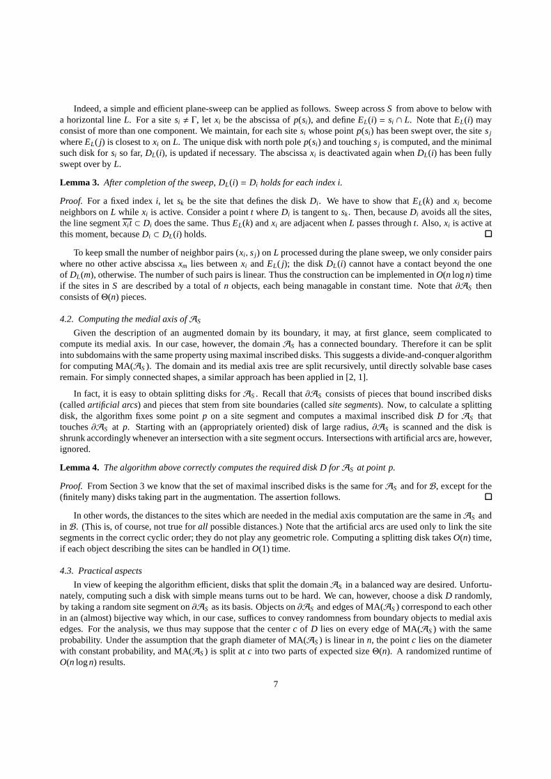
n atomic steps ration log2 n ration(log2 n)2

507 6620 1.45 0.162070 32892 1.44 0.135196 91649 1.43 0.12

10474 199001 1.42 0.1120488 417839 1.42 0.10

172198 4223178 1.41 0.09

Table 1: Five complex sites bounded byn circular arcs

n atomic steps ration log2 n ration(log2 n)2

400 7591 2.20 0.252000 54662 2.49 0.234000 143391 3.00 0.25

20000 1015149 3.55 0.2540000 2659149 4.35 0.28

200000 19820012 5.63 0.32

Table 2: Uniform distribution ofn point sites

The assumption above is realistic in scenarios where a smallnumber of sites is represented by a large numberof individual objects. The required accuracy for approximating the sites then typically leads to an input size that isindependent from the branching of MA(AS). In particular, if biarcs are used for approximation (see Section 5) thenthe number of leaves (hence also the number of vertices) of MA(AS) is determined by the original sites and not bythe number of biarcs used. Our tests report small constants in theO(n logn) term in this case. See Table 1, where stepcounts are averaged (and rounded) over 40 different equal-sized inputs.

The other extreme is the case ofn point sites. Here, by the way howAS is constructed, the diameter of MA(AS)will be typically much smaller, because many long ‘vertical’ branches will emanate from the surrounding circleΓ. Asa simple heuristic, we may choose a small number of splittingdisks tangent toΓ first, and continue with randomlysplitting the resulting augmented subdomains. This (almost) yields an observedO(n log2 n) behavior, with very smallfactors; see Table 2. We took uniformly distributed point sites — an input likely to avoid long paths in MA(AS) andthus slowing down the algorithm. Note that, for point sites,MA(AS) is basically the (piecewise-linear) medial axisof a union of disks, the augmenting disks plus the splitting disks.

Domain splitting could be combined with local tracing (i.e., traversing medial axis pieces in a consecutive manner),as done in [2], to guarantee anO(n

√n) expected time. However, the simple randomized version performed best in

all our tests. We implemented the algorithm to accept circular arc input in its current version, including (thoughnot optimizing) the handling of line segments and points. The Voronoi diagrams in Figures 1a and 1b, and also thestructures in Figures 2a and 2b as well as in Figures 9 and 10 inSubsection 6.2 have been produced by this code.

An excerpt of our experiments for point sites and circular arcs is given in Table 1 and Table 2. For input sizen,the number of atomic steps is listed along with its ratio to the functionsn log2 n andn(log2 n)2.

The atomic step needed in Subsections 4.1 and 4.2 is an intersection test of a site-describing object and a givendisk. This is among the simplest imaginable tests when a closest-site Voronoi diagram is to be computed by meansof distance calculations. Neither circles touching three given sites, nor intersection points of two bisectors, have tobe calculated, apart from (but only if desired in) the base cases delivered by divide-and-conquer. This reduces thenumerical effort and liability to errors caused by such operations, whichthemselves get rapidly complicated withthe algebraic complexity of the sites; see e.g. [11]. We usedCGAL [5] to implement the atomic operation for sitesdescribed by circular arcs (the intersection of two given circles).

8

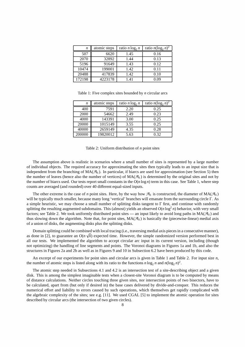
n ALG CGAL

1714 0.3 6.35622 1.1 42.6

25210 4.7 651.6116460 23.5 19650.5250366 57.8 > 24 h537360 131.1 > 1 week

(a) 40 complex sites

n ALG CGAL

100 0.14 0.26500 0.8 1.5

1000 2.2 3.15000 13.7 18.5

10000 39.3 37.650000 395.3 201.6

(b) Many small sites

Table 3: Comparison to CGAL demo program. The sites are polygonal and are bounded by a total ofn line segments.Runtimes are measured in seconds.

Table 3 displays the CPU times in seconds we measured for polygonal sites as input to our algorithm (columnsALG), in comparison to the relevant CGAL demo package for polygons (columns CGAL). While our algorithm isway faster in the case of few but large sites, the behavior of both implementations is similar in the case of many smallsites.

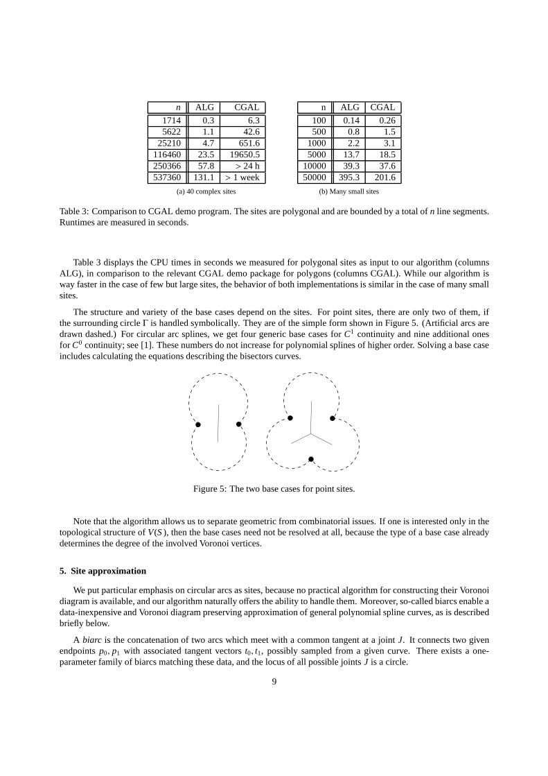
The structure and variety of the base cases depend on the sites. For point sites, there are only two of them, ifthe surrounding circleΓ is handled symbolically. They are of the simple form shown inFigure 5. (Artificial arcs aredrawn dashed.) For circular arc splines, we get four genericbase cases forC1 continuity and nine additional onesfor C0 continuity; see [1]. These numbers do not increase for polynomial splines of higher order. Solving a base caseincludes calculating the equations describing the bisectors curves.

Figure 5: The two base cases for point sites.

Note that the algorithm allows us to separate geometric fromcombinatorial issues. If one is interested only in thetopological structure ofV(S), then the base cases need not be resolved at all, because thetype of a base case alreadydetermines the degree of the involved Voronoi vertices.

5. Site approximation

We put particular emphasis on circular arcs as sites, because no practical algorithm for constructing their Voronoidiagram is available, and our algorithm naturally offers the ability to handle them. Moreover, so-called biarcs enable adata-inexpensive and Voronoi diagram preserving approximation of general polynomial spline curves, as is describedbriefly below.

A biarc is the concatenation of two arcs which meet with a common tangent at a jointJ. It connects two givenendpointsp0, p1 with associated tangent vectorst0, t1, possibly sampled from a given curve. There exists a one-parameter family of biarcs matching these data, and the locus of all possible jointsJ is a circle.

9

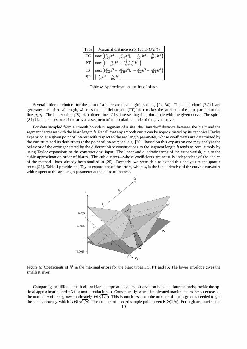
Type Maximal distance error (up toO(h5))

EC max(

| κ1324h3 − κ21944h

4|, | − κ1324h

3 − 7κ21944h

4|)

PT max(

| ± κ1324h

3 +6κ21−κ0κ21944κ0

h4|)

IS max(

| κ1324h3 +7κ2

3888h4|, | − κ1

324h3 − 5κ2

3888h4|)

SP∣

∣

∣− κ196h3 − κ2192h

4∣

∣

∣

Table 4: Approximation quality of biarcs

Several different choices for the joint of a biarc are meaningful; see e.g. [24, 30]. The equal chord (EC) biarcgenerates arcs of equal length, whereas the parallel tangent (PT) biarc makes the tangent at the joint parallel to theline p0p1. The intersection (IS) biarc determinesJ by intersecting the joint circle with the given curve. The spiral(SP) biarc chooses one of the arcs as a segment of an osculating circle of the given curve.

For data sampled from a smooth boundary segment of a site, theHausdorff distance between the biarc and thesegment decreases with the biarc lengthh. Recall that any smooth curve can be approximated by its canonical Taylorexpansion at a given point of interest with respect to the arclength parameter, whose coefficients are determined bythe curvature and its derivatives at the point of interest; see, e.g. [20]. Based on this expansion one may analyze thebehavior of the error generated by the different biarc constructions as the segment lengthh tends to zero, simply byusing Taylor expansions of the constructions’ input. The linear and quadratic terms of the error vanish, due to thecubic approximation order of biarcs. The cubic terms—whosecoefficients are actually independent of the choiceof the method—have already been studied in [25]. Recently, we were able to extend this analysis to the quarticterms [26]. Table 4 provides the Taylor expansions of the errors, whereκi is thei-th derivative of the curve’s curvaturewith respect to the arc length parameter at the point of interest.

0

0

0

1

1

2

2

0.0025

0.005

−0.0025

κ2

κ21κ0

h

IS

PT

EC

Figure 6: Coefficients ofh4 in the maximal errors for the biarc types EC, PT and IS. The lower envelope gives thesmallest error.

Comparing the different methods for biarc interpolation, a first observation is that all four methods provide the op-timal approximation order 3 (for non-circular input). Consequently, when the tolerated maximum errorε is decreased,the numbern of arcs grows moderately,Θ( 3

√1/ε). This is much less than the number of line segments needed toget

the same accuracy, which isΘ(√

1/ε). The number of needed sample points even isΘ(1/ε). For high accuracies, the10

⋆

⋆⋆

⋆

∂Aδ

∂AA

Aδ

A1

A1

A2

A2

e2

A3e3

A4

e4

A5

A6e6

A7

D(x, δ)

Aδ2

(a) (b) (c) (d)

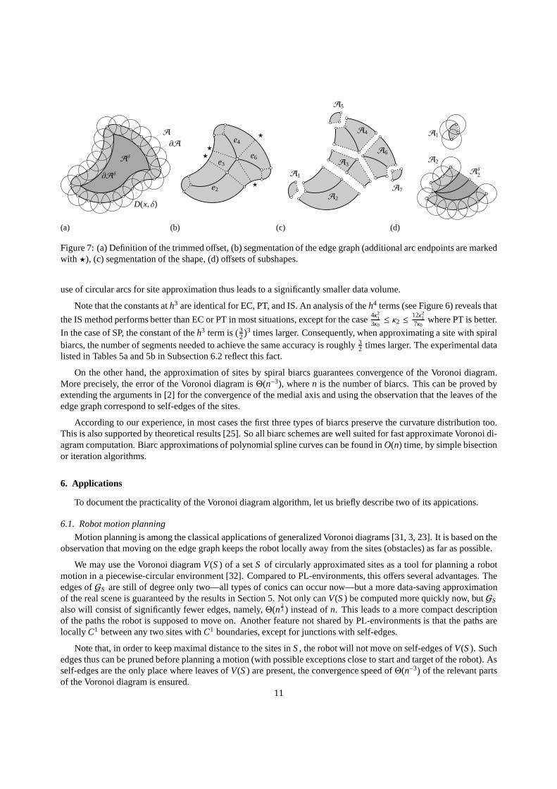
Figure 7: (a) Definition of the trimmed offset, (b) segmentation of the edge graph (additional arc endpoints are markedwith ⋆), (c) segmentation of the shape, (d) offsets of subshapes.

use of circular arcs for site approximation thus leads to a significantly smaller data volume.

Note that the constants ath3 are identical for EC, PT, and IS. An analysis of theh4 terms (see Figure 6) reveals that

the IS method performs better than EC or PT in most situations, except for the case4κ213κ0≤ κ2 ≤

12κ217κ0

where PT is better.

In the case of SP, the constant of theh3 term is (32)3 times larger. Consequently, when approximating a site withspiralbiarcs, the number of segments needed to achieve the same accuracy is roughly3

2 times larger. The experimental datalisted in Tables 5a and 5b in Subsection 6.2 reflect this fact.

On the other hand, the approximation of sites by spiral biarcs guarantees convergence of the Voronoi diagram.More precisely, the error of the Voronoi diagram isΘ(n−3), wheren is the number of biarcs. This can be proved byextending the arguments in [2] for the convergence of the medial axis and using the observation that the leaves of theedge graph correspond to self-edges of the sites.

According to our experience, in most cases the first three types of biarcs preserve the curvature distribution too.This is also supported by theoretical results [25]. So all biarc schemes are well suited for fast approximate Voronoi di-agram computation. Biarc approximations of polynomial spline curves can be found inO(n) time, by simple bisectionor iteration algorithms.

6. Applications

To document the practicality of the Voronoi diagram algorithm, let us briefly describe two of its appications.

6.1. Robot motion planning

Motion planning is among the classical applications of generalized Voronoi diagrams [31, 3, 23]. It is based on theobservation that moving on the edge graph keeps the robot locally away from the sites (obstacles) as far as possible.

We may use the Voronoi diagramV(S) of a setS of circularly approximated sites as a tool for planning a robotmotion in a piecewise-circular environment [32]. Comparedto PL-environments, this offers several advantages. Theedges ofGS are still of degree only two—all types of conics can occur now—but a more data-saving approximationof the real scene is guaranteed by the results in Section 5. Not only canV(S) be computed more quickly now, butGS

also will consist of significantly fewer edges, namely,Θ(n23 ) instead ofn. This leads to a more compact description

of the paths the robot is supposed to move on. Another featurenot shared by PL-environments is that the paths arelocally C1 between any two sites withC1 boundaries, except for junctions with self-edges.

Note that, in order to keep maximal distance to the sites inS, the robot will not move on self-edges ofV(S). Suchedges thus can be pruned before planning a motion (with possible exceptions close to start and target of the robot). Asself-edges are the only place where leaves ofV(S) are present, the convergence speed ofΘ(n−3) of the relevant partsof the Voronoi diagram is ensured.

11

a1i a1

ia1

i

a1i

c1i

c1i

c1i

c1i

⋆⋆

⋆

⋆

⋆

⋆

⋆

⋆

a2i

a2ia2

ia2

i

c2i

c2i

c2i

c2i

(a) (b) (c) (d)

Figure 8: Splitting subshapes into monotonic pieces. The centers of the arcsa1i , a

2i span the dashed lines.

6.2. Trimmed offsets

Offsetting is a fundamental operation for planar shapes, and itis needed frequently, e.g., in computer-aidedmanufacturing [16, 27]. Several authors base their offsetting algorithms on the Voronoi diagram or the medialaxis [16, 13, 4]. Once more, a PC-representation of the inputshape is advantageous, because the class of suchshapes is closed under offsetting operations.

Our Voronoi diagram algorithm is particularly well suited to this task, because it delivers the necessary combina-torial structure without computing the edge graph explicitly. Depending on the application, we can compute the inneror the outer offset of a given planar shapeA. For inner offsets, we take the outer boundary ofA as the surroundingcurve (replacing the circleΓ) and the holes ofA as the sites. For outer offsets, we compute the inner offsets of thecomplement ofA within a suitable disk coveringA.

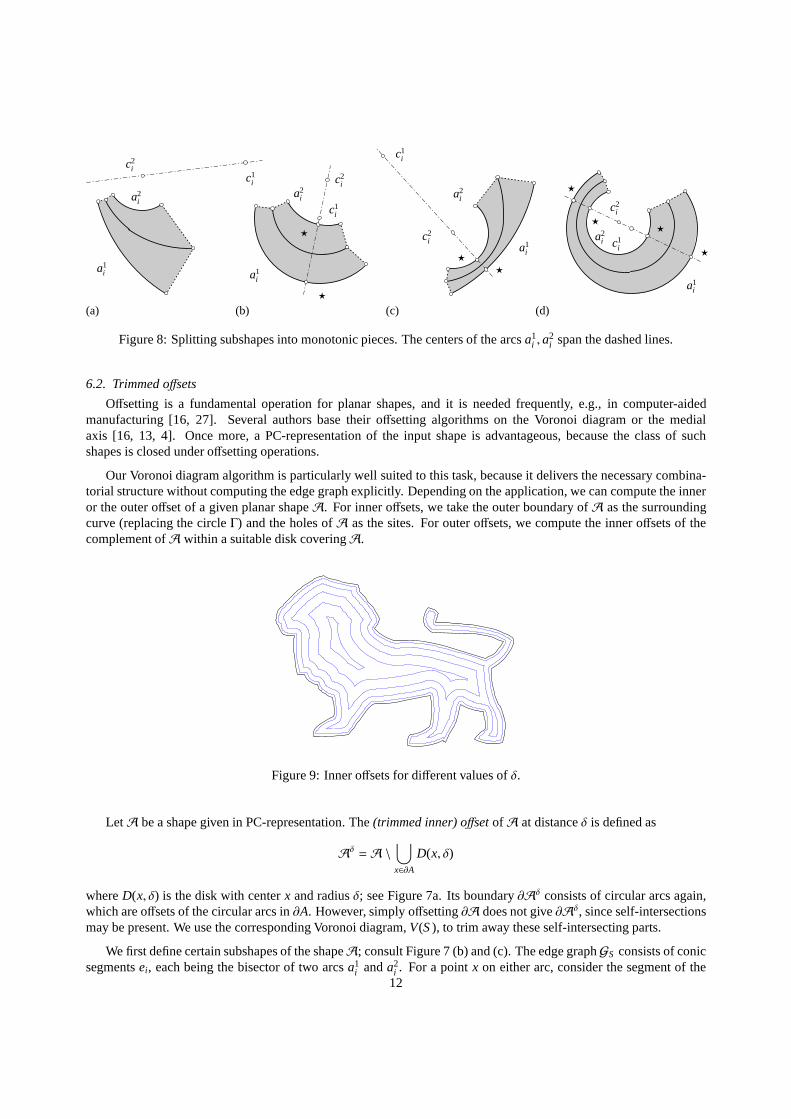
Figure 9: Inner offsets for different values ofδ.

LetA be a shape given in PC-representation. The(trimmed inner) offsetofA at distanceδ is defined as

Aδ = A \⋃

x∈∂AD(x, δ)

whereD(x, δ) is the disk with centerx and radiusδ; see Figure 7a. Its boundary∂Aδ consists of circular arcs again,which are offsets of the circular arcs in∂A. However, simply offsetting∂A does not give∂Aδ, since self-intersectionsmay be present. We use the corresponding Voronoi diagram,V(S), to trim away these self-intersecting parts.

We first define certain subshapes of the shapeA; consult Figure 7 (b) and (c). The edge graphGS consists of conicsegmentsei , each being the bisector of two arcsa1

i anda2i . For a pointx on either arc, consider the segment of the

12

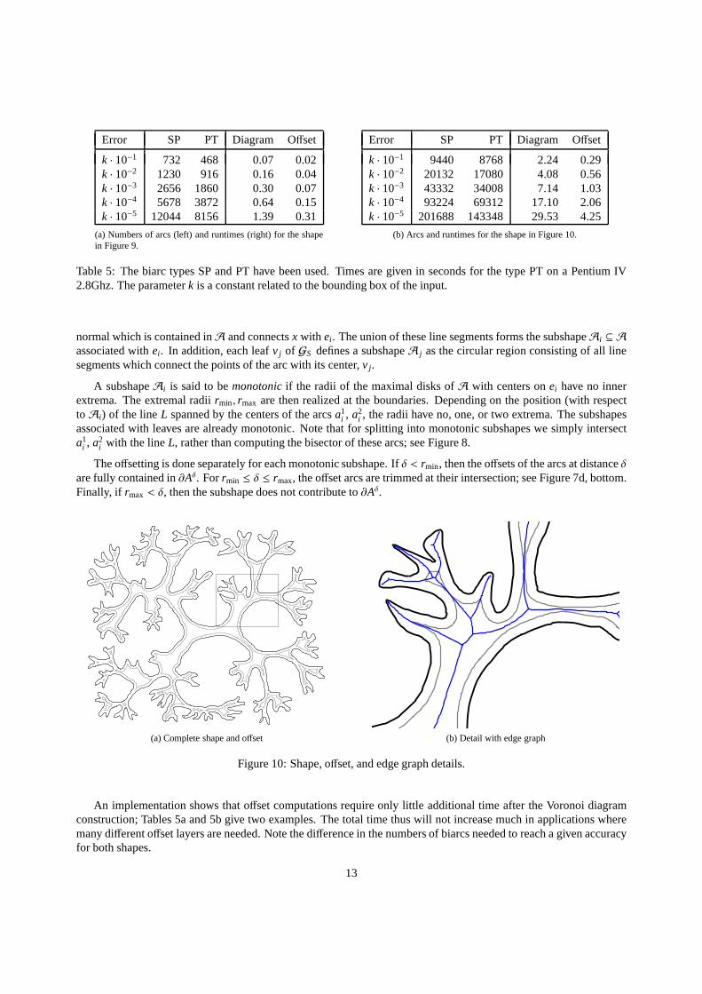
Error SP PT Diagram Offset

k · 10−1 732 468 0.07 0.02k · 10−2 1230 916 0.16 0.04k · 10−3 2656 1860 0.30 0.07k · 10−4 5678 3872 0.64 0.15k · 10−5 12044 8156 1.39 0.31

(a) Numbers of arcs (left) and runtimes (right) for the shapein Figure 9.

Error SP PT Diagram Offset

k · 10−1 9440 8768 2.24 0.29k · 10−2 20132 17080 4.08 0.56k · 10−3 43332 34008 7.14 1.03k · 10−4 93224 69312 17.10 2.06k · 10−5 201688 143348 29.53 4.25

(b) Arcs and runtimes for the shape in Figure 10.

Table 5: The biarc types SP and PT have been used. Times are given in seconds for the type PT on a Pentium IV2.8Ghz. The parameterk is a constant related to the bounding box of the input.

normal which is contained inA and connectsx with ei . The union of these line segments forms the subshapeAi ⊆ Aassociated withei . In addition, each leafv j of GS defines a subshapeA j as the circular region consisting of all linesegments which connect the points of the arc with its center,v j.

A subshapeAi is said to bemonotonicif the radii of the maximal disks ofA with centers onei have no innerextrema. The extremal radiirmin, rmax are then realized at the boundaries. Depending on the position (with respecttoAi) of the lineL spanned by the centers of the arcsa1

i , a2i , the radii have no, one, or two extrema. The subshapes

associated with leaves are already monotonic. Note that forsplitting into monotonic subshapes we simply intersecta1

i , a2i with the lineL, rather than computing the bisector of these arcs; see Figure 8.

The offsetting is done separately for each monotonic subshape. Ifδ < rmin, then the offsets of the arcs at distanceδare fully contained in∂Aδ. Forrmin ≤ δ ≤ rmax, the offset arcs are trimmed at their intersection; see Figure 7d, bottom.Finally, if rmax < δ, then the subshape does not contribute to∂Aδ.

(a) Complete shape and offset (b) Detail with edge graph

Figure 10: Shape, offset, and edge graph details.

An implementation shows that offset computations require only little additional time afterthe Voronoi diagramconstruction; Tables 5a and 5b give two examples. The total time thus will not increase much in applications wheremany different offset layers are needed. Note the difference in the numbers of biarcs needed to reach a given accuracyfor both shapes.

13

7. Concluding remarks

We have presented a simple and practical divide-and-conquer algorithm for computing Voronoi diagrams forgeneral sites in the plane. The primary aim of this work has been establishing an approach which allows for an easyand robust implementation. Thus, the emphasis of our CGAL-based implementation has been put more on simplicityand straightforwardness than on runtime optimization. Nevertheless, the program achieves an observed runtime ofO(n logn) with small constants when computing the edge graph for setsof large and complex sites. For sets withmany small sites we roughly obtain anO(n log2 n) behaviour with the help of simple heuristics. By choosing thesplitting disks in a more sophisticated way when dealing with heavily branched Voronoi diagrams, and by moreelaborate implementation, we believe that a substantiallybetter behaviour may be achieved for the case of small sites(in particular, for point sites). The simple, fully implemented version of the program has already proven to be easilyadaptable to some problems classically related to Voronoi diagrams. Examples are offset computation and robotmotion planning. Especially our offset solution takes advantage of the combinatorial representation of the diagram wecompute, which is, together with the generality of the approach, one of the major features which sets our algorithmapart from most other state-of-the-art algorithms in this area.

References

[1] O. Aichholzer, W. Aigner, F. Aurenhammer, T. Hackl, B. J¨uttler, and M. Rabl. Medial axis computation for planar free-form shapes.Computer-Aided Design, in press.

[2] O. Aichholzer, F. Aurenhammer, T. Hackl, B. Juttler, M.Oberneder, and Z.Sır. Computational and structural advantages of circularboundaryrepresentation. InSpringer Lecture Notes in Computer Science, volume 4619, pages 374–385, 2007.

[3] H. Alt, O. Cheong, and A. Vigneron. The Voronoi diagram ofcurved objects.Discrete& Computational Geometry, 34:439–453, 2005.[4] L. Cao and J. Liu. Computation of medial axis and offset curves of curved boundaries in planar domain.Computer-Aided Design, 40(4):465–

475, 2008.[5] CGAL. Computational Geometry Algorithms Library. http://www.cgal.org/.[6] B. Chazelle. A theorem on polygon cutting with applications. InProc. 23rd Ann. IEEE Symp. Foundations of Computer Science, pages

339–349, 1982.[7] L.P. Chew and R.L. Drysdale. Voronoi diagrams based on convex distance functions. InProc. 1st Ann. ACM Symposium on Computational

Geometry, pages 235–244, 1985.[8] F.Y.L. Chin, J. Snoeyink, and C.A. Wang. Finding the medial axis of a simple polygon in linear time.Discrete& Computational Geometry,

21:405–420, 1999.[9] H.I. Choi, S.W. Choi, and H.P. Moon. Mathematical theoryof medial axis transform.Pacific Journal of Mathematics, 181:57–88, 1997.

[10] G. Elber, E. Cohen, and S. Drake. MATHSM: Medial axis transform toward high speed machining of pockets.Computer-Aided Design,37:241–250, 2005.

[11] I.Z. Emiris, E.P. Tsigaridas, and G.M. Tzoumas. The predicates for the Voronoi diagram of ellipses. InProc. 22nd Ann. ACM Symposium onComputational Geometry, pages 227–236, 2006.

[12] S. Fortune. A sweep line algorithm for Voronoi diagrams. Algorithmica, 2:153–174, 1987.[13] M. Held. Voronoi diagrams and offset curves of curvilinear polygons.Computer-Aided Design, 30(4):287–300, 1998.[14] M. Held. VRONI: An engineering approach to the reliableand efficient computation of Voronoi diagrams of points and line segments.

Computational Geometry: Theory and Applications, 18(2):95–123, 2001.[15] M. Held, and S. Huber. Topology-oriented incremental computation of Voronoi diagrams of circular arcs and straight line segments.

Computer-Aided Design, in press.[16] M. Held, G. Lukacs, and L. Andor. Pocket machining basedon contour-parallel tool paths generated by means of proximity maps.Computer-

Aided Design, 26(3):189–203, 1994.[17] D.G. Kirkpatrick. Efficient computation of continuous skeletons. InProc. 20th Ann. IEEE Symp. Foundations of Computer Science, pages

18–27, 1979.[18] R. Klein. Concrete and Abstract Voronoi diagrams. Springer Lecture Notes in Computer Science 400, 1990.[19] R. Klein, K. Mehlhorn, and S. Meiser. Randomized incremental construction of abstract Voronoi diagrams.Computational Geometry:

Theory and Applications, 3:157–184, 1993.[20] E. Kreyszig. Differential Geometry, Dover, New York, 1991.[21] D.T. Lee. Medial axis transformation of a planar shape.IEEE Trans. Pattern Analysis and Machine Intelligence, 4:363–369, 1982.[22] D.T. Lee and R.L.S. Drysdale. Generalization of Voronoi diagrams in the plane.SIAM Journal on Computing, 10:73–87, 1981.[23] M. McAllister, D. Kirkpatrick, and J. Snoeyink. A compact piecewise-linear Voronoi diagram for convex sites in theplane. Discrete&

Computational Geometry, 15:73–105, 1996.[24] D. S. Meek and D. J. Walton. Spiral arc spline approximation to a planar spiral.J. Comput. Appl. Math., 107:21–30, 1999.[25] D.S. Meek and D.J. Walton. Approximating smooth planarcurves by arc splines.J. Comput. Appl. Math., 59:221–231, 1995.[26] E. Pilgerstorfer. Asymptotischer Vergleich verschiedener Verfahren der Biarc-Approximation.Master Thesis, Johannes Kepler University

Linz, Austria, 2008.[27] J-K. Seong, G. Elber, and M-S. Kim. Trimming local and global self-intersections in offset curves/surfaces using distance maps.Computer-

Aided Design, 38:183–193, 2006.

14

[28] M.I. Shamos and D. Hoey. Closest-point problems. InProc. 16th Ann. IEEE Symp. Foundations of Computer Science, pages 151–162, 1975.[29] M. Sharir. Intersection and closest-pair problems fora set of circular discs.SIAM Journal on Computing, 14:448–468, 1985.[30] Z. Sır, R. Feichtinger, and B. Juttler. Approximating curves and their offsets using biarcs and Pythagorean hodograph quintics.Computer-

Aided Design, 38:608–618, 2006.[31] C.-K. Yap. An O(n logn) algorithm for the Voronoi diagram of a set of simple curve segments. Discrete& Computational Geometry,

2:365–393, 1987.[32] C.-K. Yap and H. Alt. Motion planning in the CL-environment. InLecture Notes In Computer Science 382, pages 373–380, 1989.

15