COSC 6114 Prof. Andy Mirzaian

Introduction

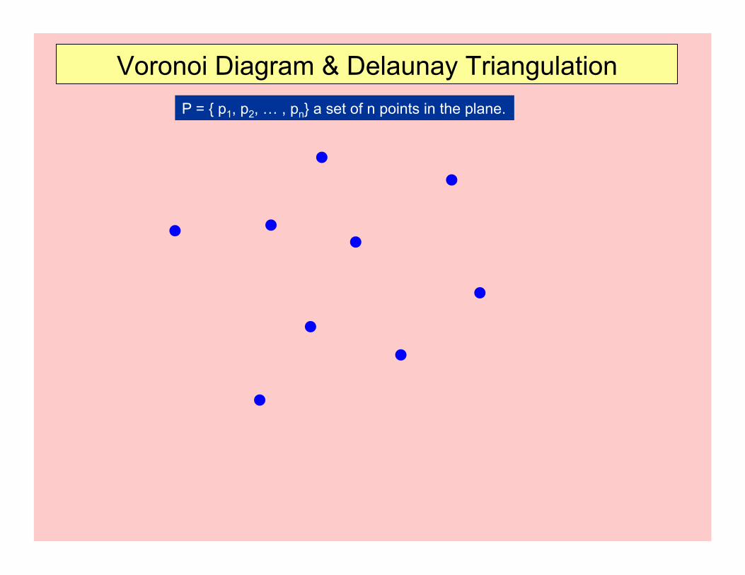
Voronoi Diagram & Delaunay Triangulation P = { p1, p2, , pn} a set of n points in the plane.

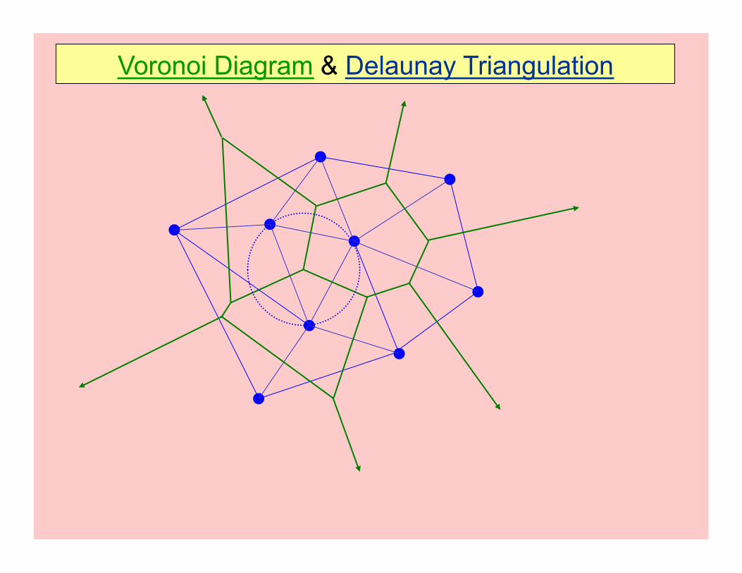
Voronoi Diagram & Delaunay Triangulation

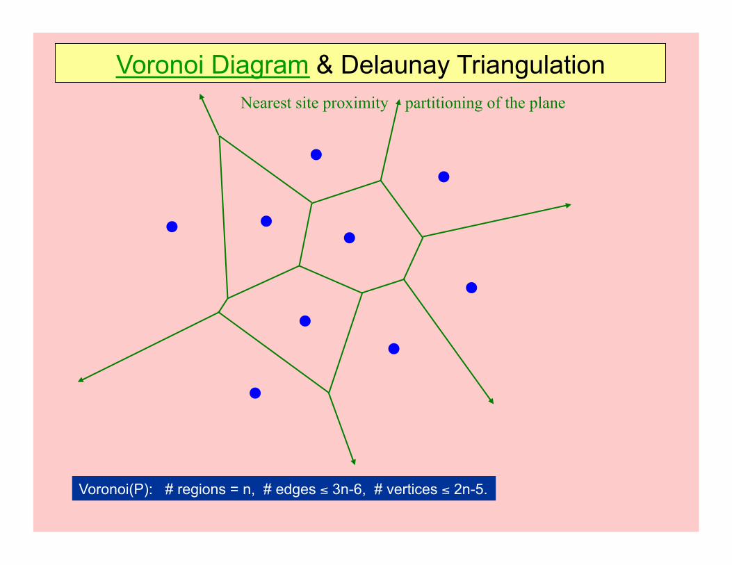
Voronoi(P): # regions = n, # edges ! 3n-6, # vertices ! 2n-5.

Nearest site proximity partitioning of the plane

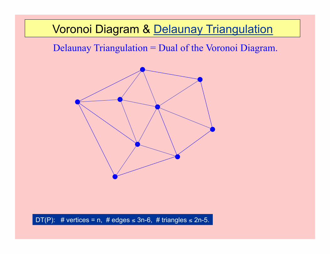
Delaunay Triangulation = Dual of the Voronoi Diagram.

Voronoi Diagram & Delaunay Triangulation

DT(P): # vertices = n, # edges ! 3n-6, # triangles ! 2n-5.

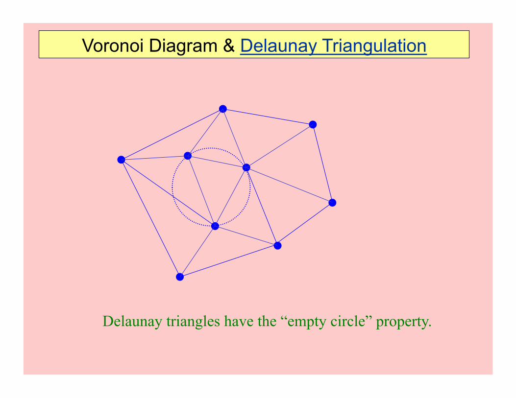
Delaunay triangles have the empty circle property.

Voronoi Diagram & Delaunay Triangulation

Voronoi Diagram & Delaunay Triangulation

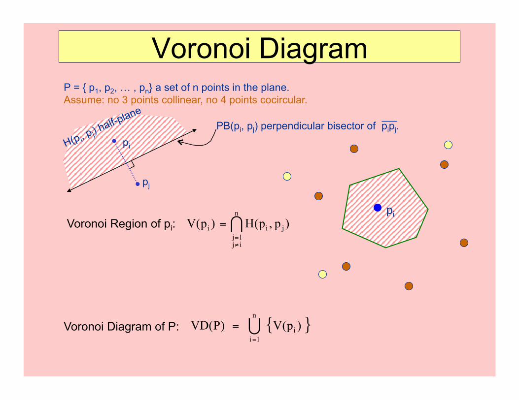
Voronoi Diagram P = { p1, p2, , pn} a set of n points in the plane. Assume: no 3 points collinear, no 4 points cocircular.

PB(pi, pj) perpendicular bisector of pipj. pi

pj

Voronoi Region of pi: pi

Voronoi Diagram of P:

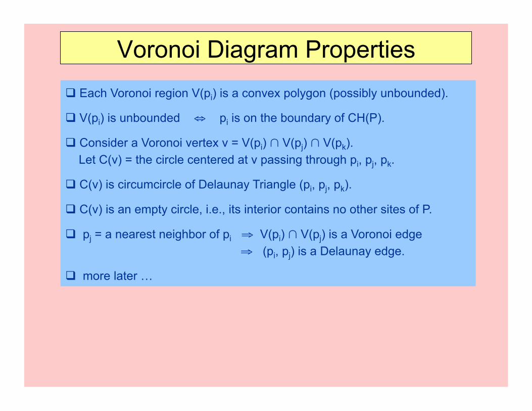
Voronoi Diagram Properties ! Each Voronoi region V(pi) is a convex polygon (possibly unbounded).

! V(pi) is unbounded " pi is on the boundary of CH(P).

! Consider a Voronoi vertex v = V(pi) # V(pj) # V(pk). Let C(v) = the circle centered at v passing through pi, pj, pk.

! C(v) is circumcircle of Delaunay Triangle (pi, pj, pk).

! C(v) is an empty circle, i.e., its interior contains no other sites of P.

! pj = a nearest neighbor of pi $ V(pi) # V(pj) is a Voronoi edge $ (pi, pj) is a Delaunay edge.

! more later

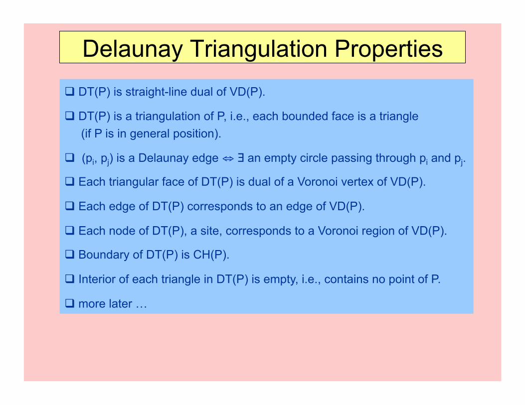
Delaunay Triangulation Properties ! DT(P) is straight-line dual of VD(P).

! DT(P) is a triangulation of P, i.e., each bounded face is a triangle (if P is in general position).

! (pi, pj) is a Delaunay edge " % an empty circle passing through pi and pj.

! Each triangular face of DT(P) is dual of a Voronoi vertex of VD(P).

! Each edge of DT(P) corresponds to an edge of VD(P).

! Each node of DT(P), a site, corresponds to a Voronoi region of VD(P).

! Boundary of DT(P) is CH(P).

! Interior of each triangle in DT(P) is empty, i.e., contains no point of P.

! more later

References: [M. de Berge et al 00] chapters 7, 9, 13

[Preparata-Shamos85] chapters 5, 6

[ORourke98] chapter 5

[Edelsbrunner87] chapter 13

AAW

Lecture Notes 16, 17, 18, 19

ALGORITHMS

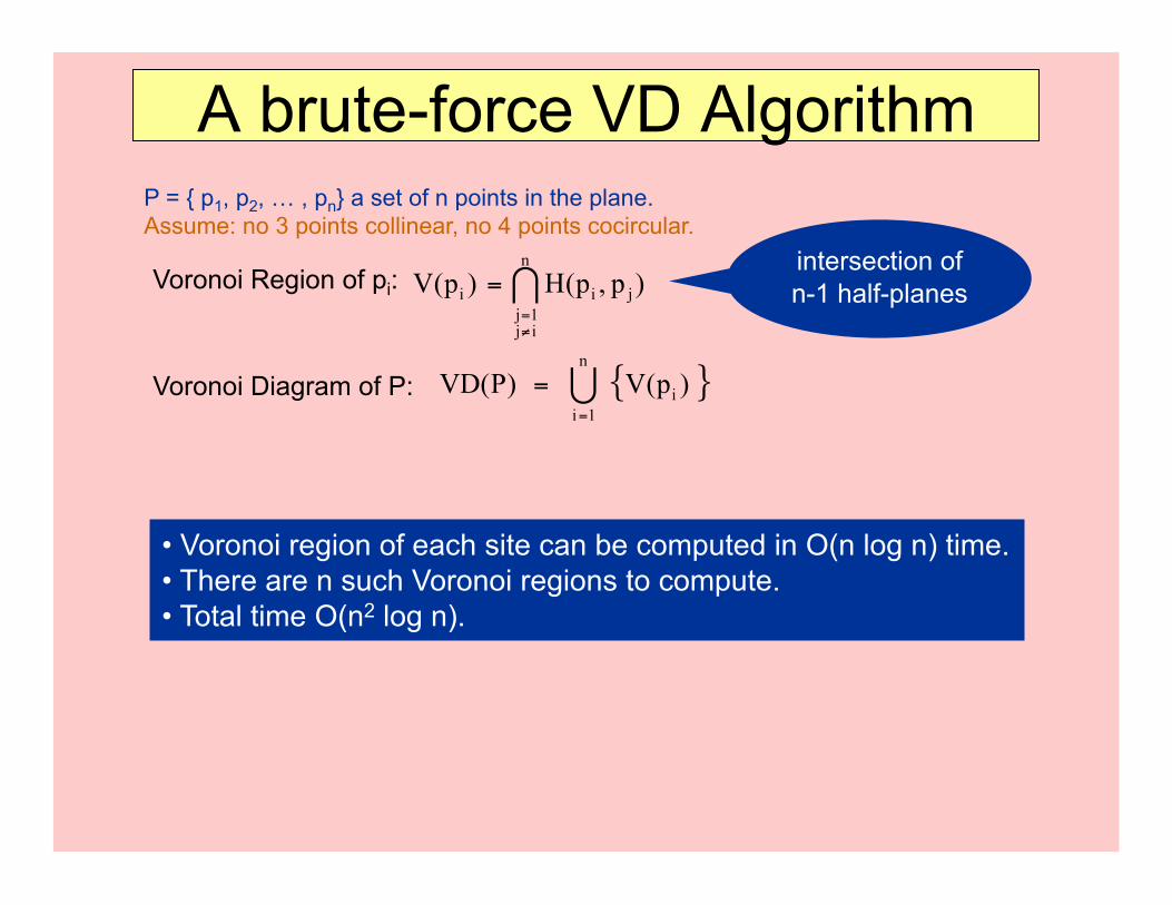
A brute-force VD Algorithm P = { p1, p2, , pn} a set of n points in the plane. Assume: no 3 points collinear, no 4 points cocircular.

Voronoi Region of pi:

Voronoi Diagram of P:

intersection of n-1 half-planes

Voronoi region of each site can be computed in O(n log n) time. There are n such Voronoi regions to compute. Total time O(n2 log n).

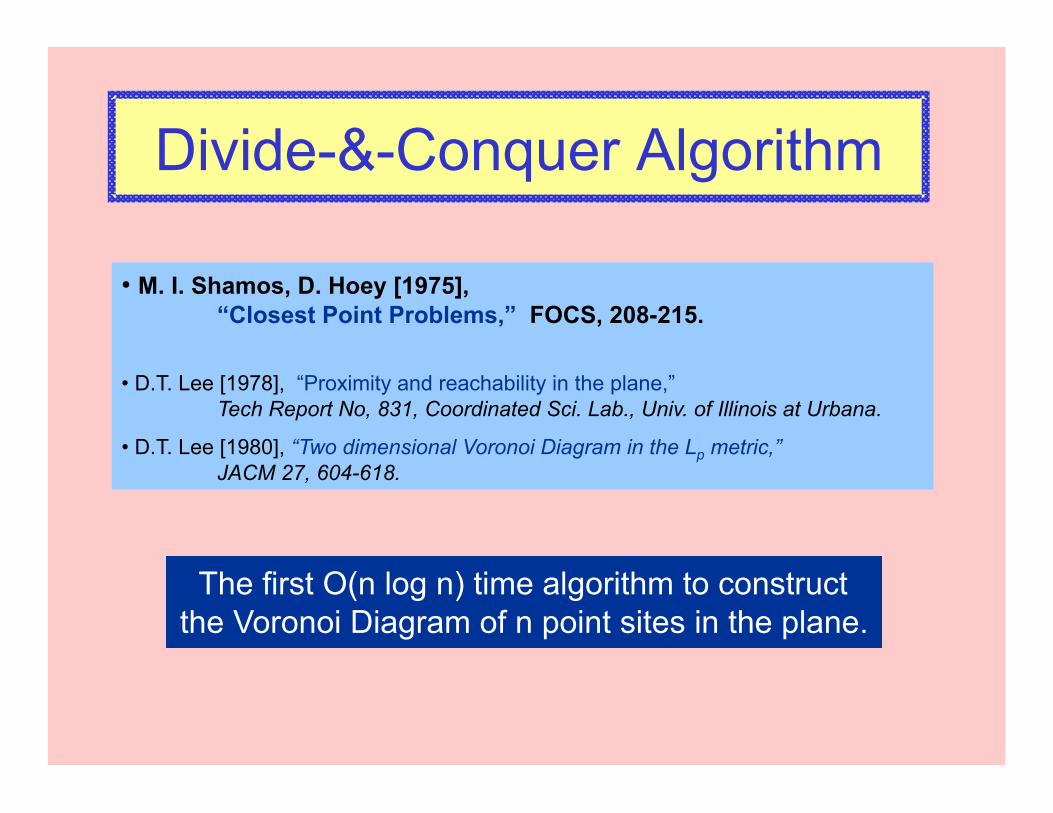
Divide-&-Conquer Algorithm

M. I. Shamos, D. Hoey [1975], Closest Point Problems, FOCS, 208-215.

D.T. Lee [1978], Proximity and reachability in the plane, Tech Report No, 831, Coordinated Sci. Lab., Univ. of Illinois at Urbana.

D.T. Lee [1980], Two dimensional Voronoi Diagram in the Lp metric, JACM 27, 604-618.

The first O(n log n) time algorithm to construct the Voronoi Diagram of n point sites in the plane.

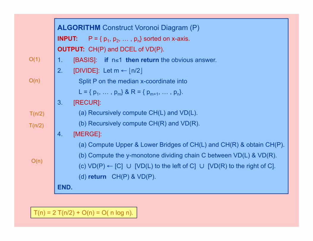
ALGORITHM Construct Voronoi Diagram (P) INPUT: P = { p1, p2, , pn} sorted on x-axis. OUTPUT: CH(P) and DCEL of VD(P). 1. [BASIS]: if n!1 then return the obvious answer. 2. [DIVIDE]: Let m & 'n/2(

Split P on the median x-coordinate into

L = { p1, , pm} & R = { pm+1, , pn}.

3. [RECUR]: (a) Recursively compute CH(L) and VD(L).

(b) Recursively compute CH(R) and VD(R).

4. [MERGE]: (a) Compute Upper & Lower Bridges of CH(L) and CH(R) & obtain CH(P).

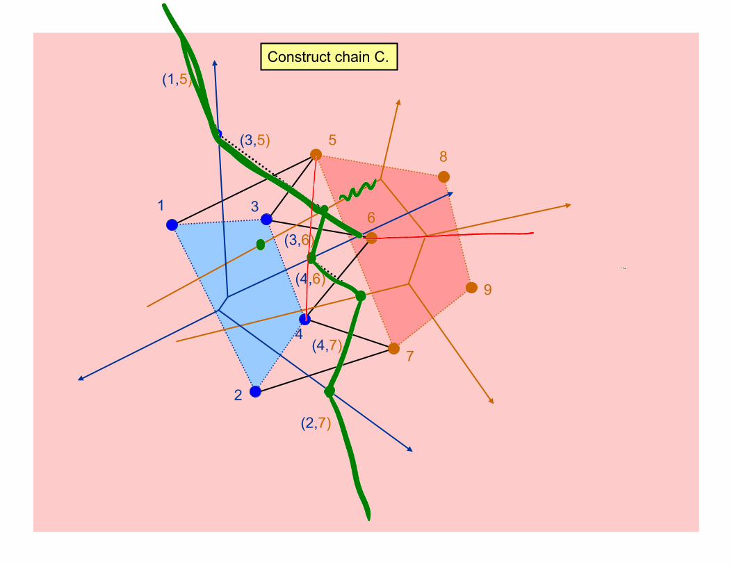
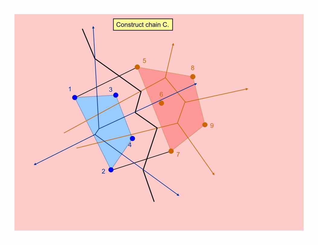
(b) Compute the y-monotone dividing chain C between VD(L) & VD(R).

(c) VD(P) & [C] ) [VD(L) to the left of C] ) [VD(R) to the right of C]. (d) return CH(P) & VD(P).

END.

O(1)

O(n)

T(n/2)

T(n/2)

O(n)

T(n) = 2 T(n/2) + O(n) = O( n log n).

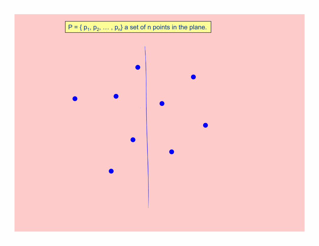
P = { p1, p2, , pn} a set of n points in the plane.

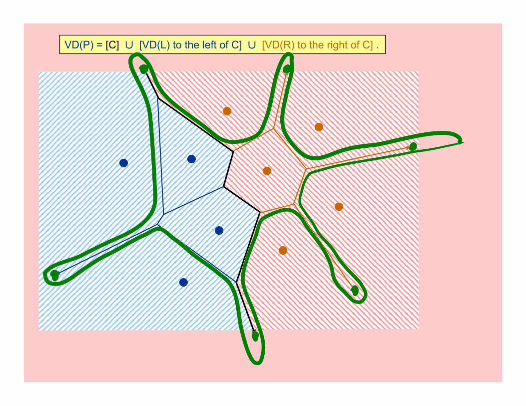
VD(P) = [C] ) [VD(L) to the left of C] ) [VD(R) to the right of C] .

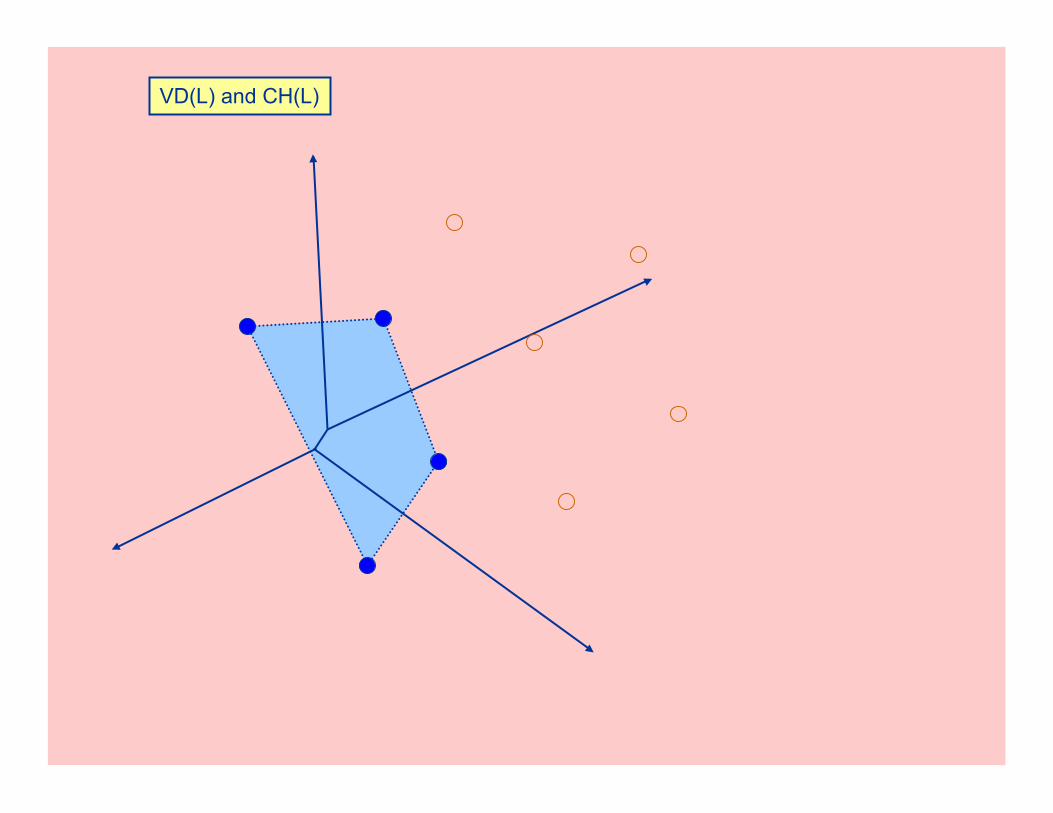
VD(L) and CH(L)

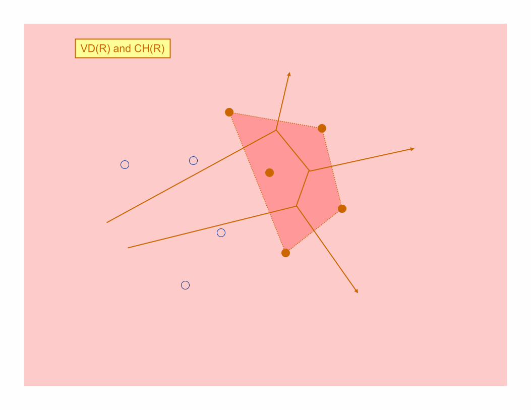
VD(R) and CH(R)

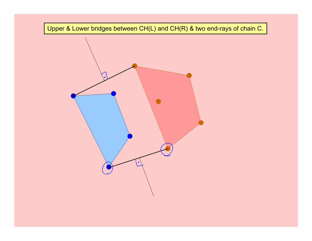
Upper & Lower bridges between CH(L) and CH(R) & two end-rays of chain C.

1

2

3

4

5

6

7

8

9

(1,5)

(3,5)

(3,6)

(4,6)

(4,7)

(2,7)

Construct chain C.

1

2

3

4

5

6

7

8

9

Construct chain C.

1

2

3

4

5

6

7

8

9

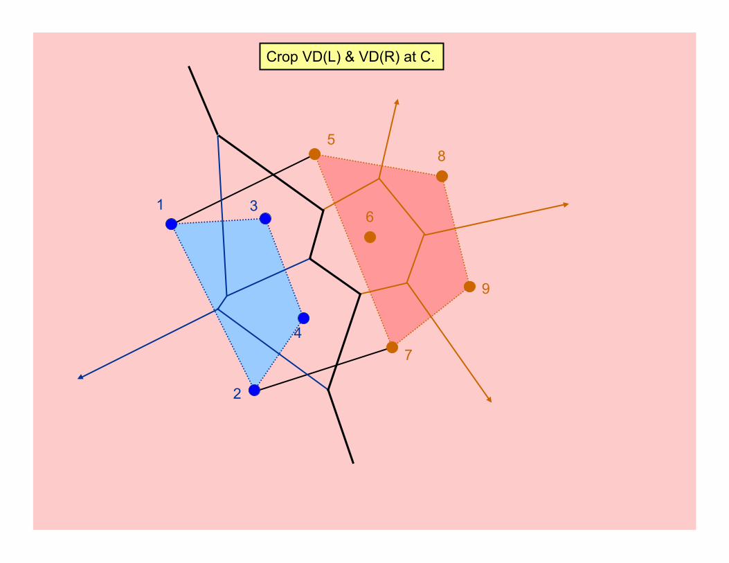
Crop VD(L) & VD(R) at C.

1

2

3

4

5

6

7

8

9

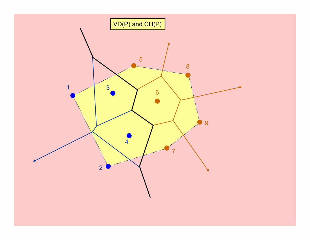
VD(P) and CH(P)

Fortunes Algorithm Steve Fortune [1987], A Sweepline algorithm for Voronoi Diagrams,

Algorithmica, 153-174.

Guibas, Stolfi [1987], Ruler, Compass and computer: The design and analysis of geometric algorithms, Proc. of the NATO Advanced Science Institute, series F, vol. 40: Theoretical Foundations of Computer Graphics and CAD, 111-165.

" O(n log n) time algorithm by plane-sweep. " See AAW animation. " Generalization: VD of line-segments and circles.

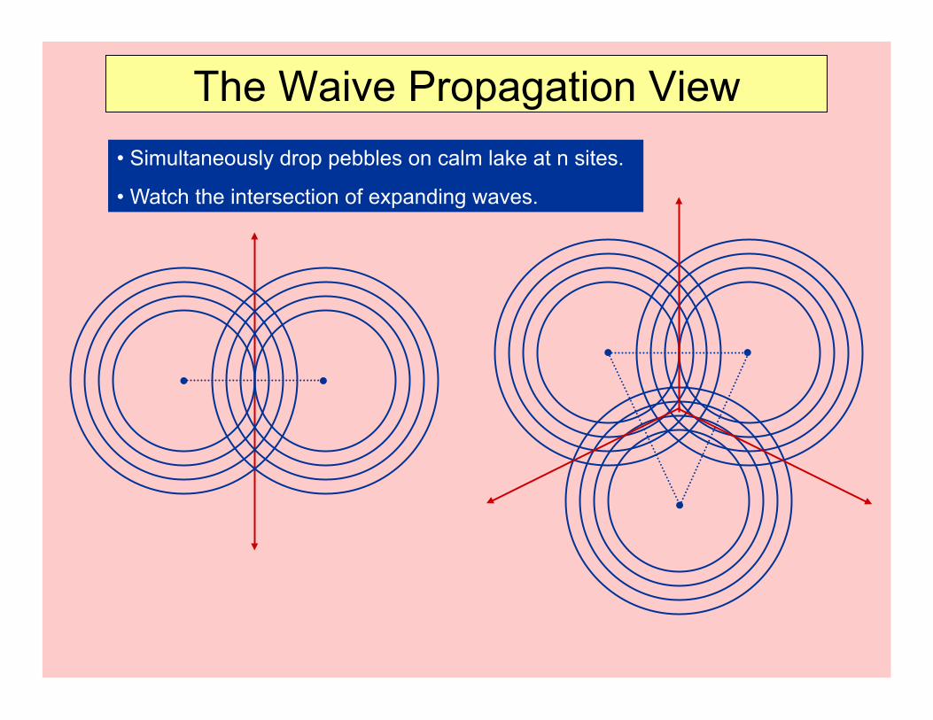
The Waive Propagation View Simultaneously drop pebbles on calm lake at n sites.

Watch the intersection of expanding waves.

Time as 3rd dimension

x

y x

z=time

y

*+ *+

p

p apex

of the cone

All sites have identical opaque cones.

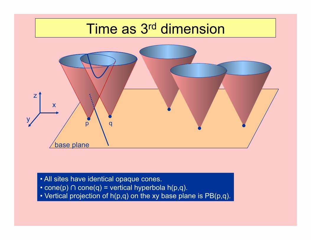
Time as 3rd dimension

x z

y

All sites have identical opaque cones. cone(p) # cone(q) = vertical hyperbola h(p,q). Vertical projection of h(p,q) on the xy base plane is PB(p,q).

p q

base plane

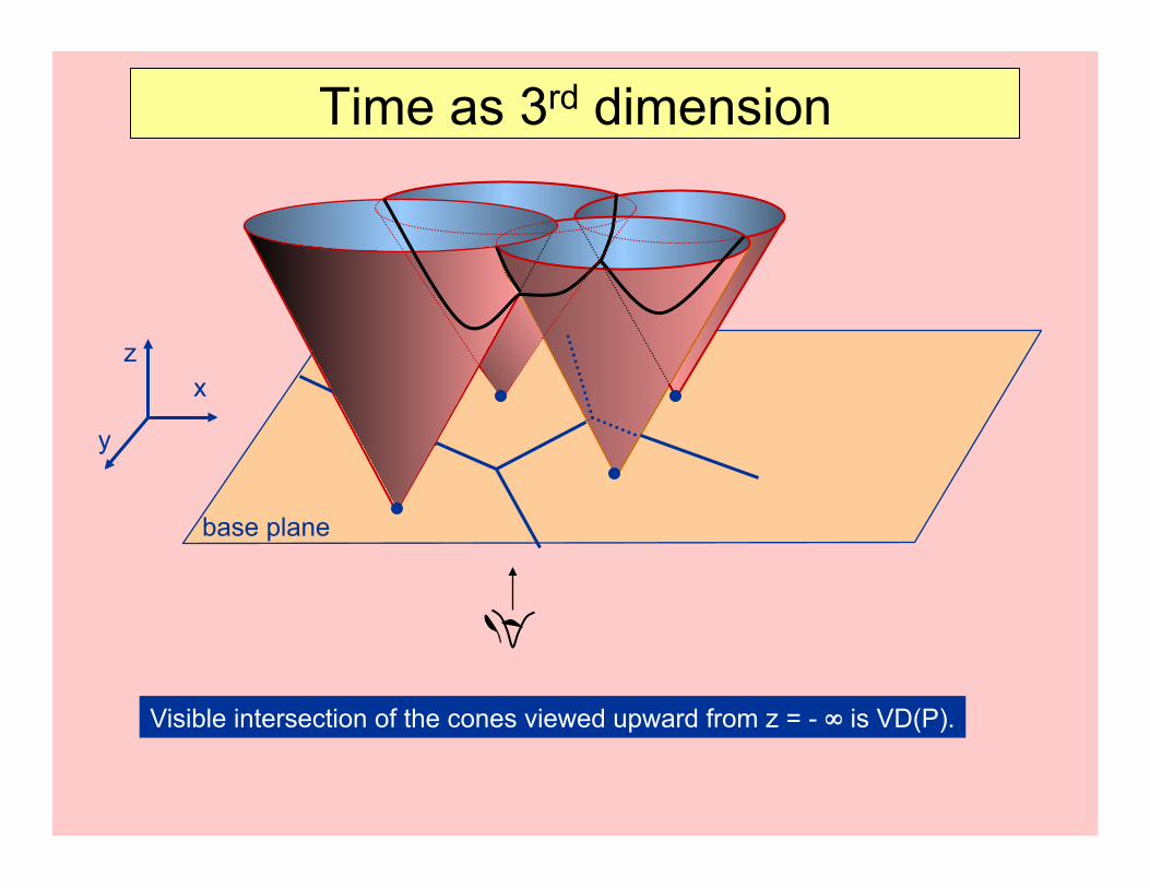
Time as 3rd dimension

x z

y

Visible intersection of the cones viewed upward from z = - , is VD(P).

base plane

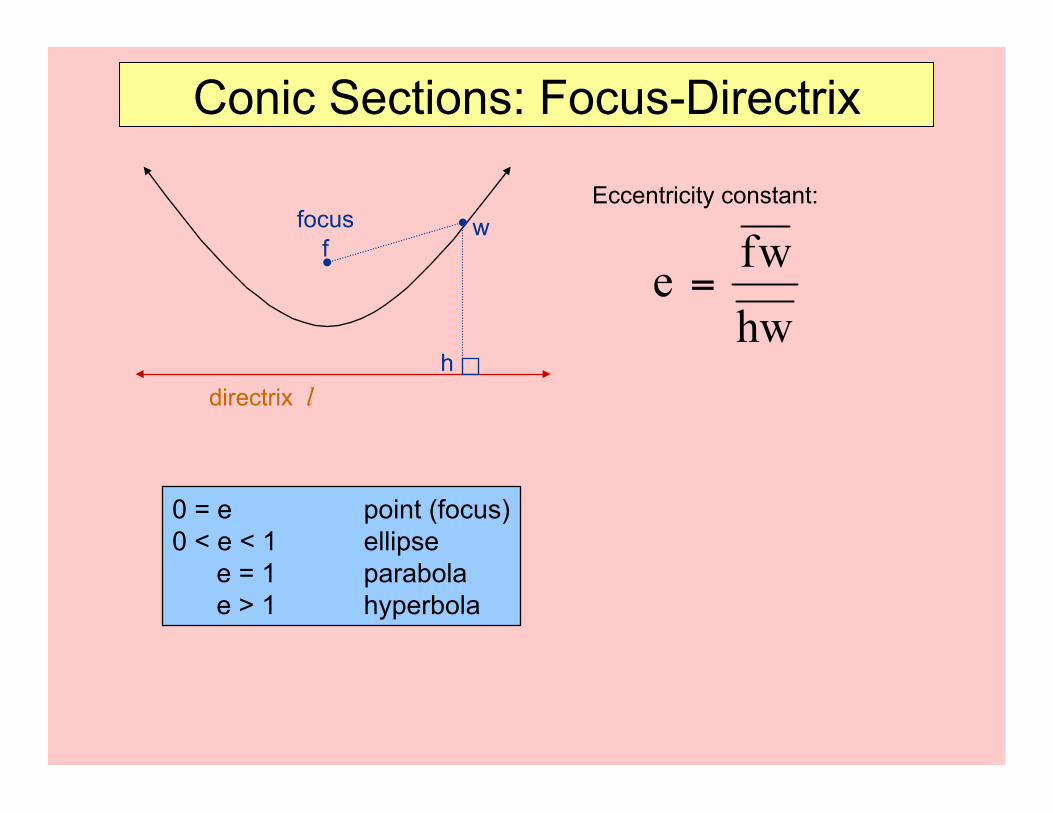
Conic Sections: Focus-Directrix

focus f

directrix l

w

h

Eccentricity constant:

0 = e point (focus) 0 < e < 1 ellipse e = 1 parabola e > 1 hyperbola

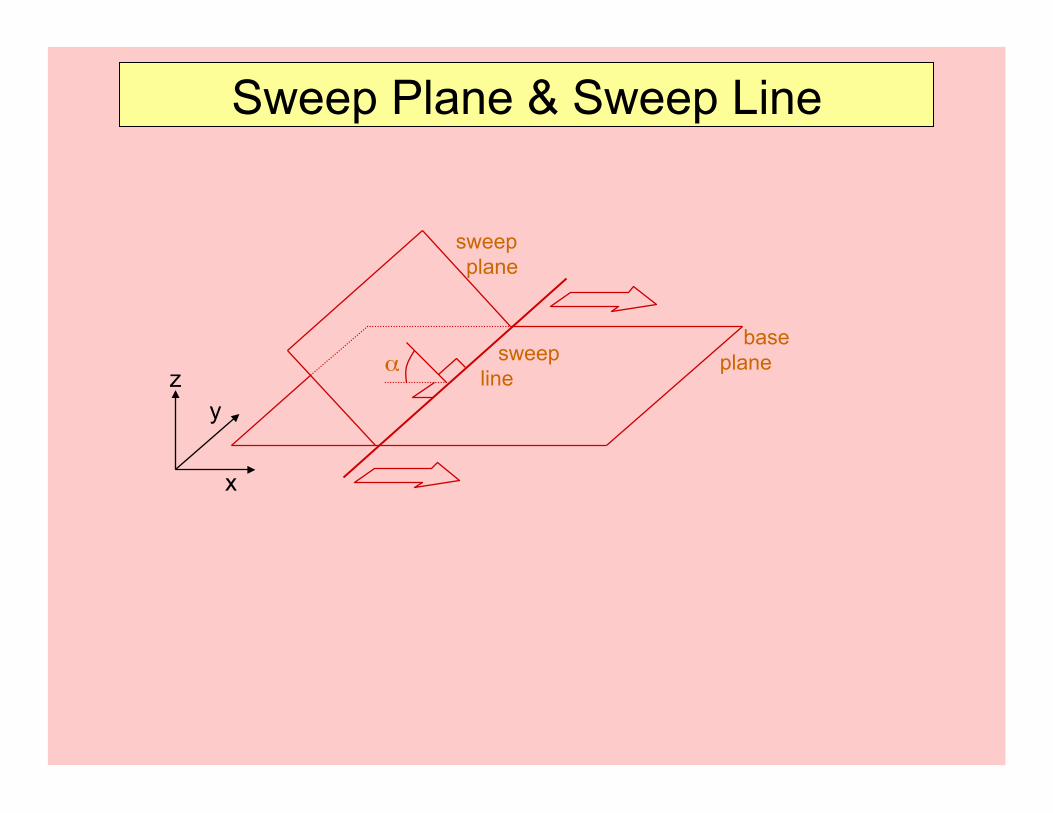
sweep plane

sweep line

*+ base plane

x

y

Sweep Plane & Sweep Line

z

sweep plane

*+*+

base plane p

v

w u

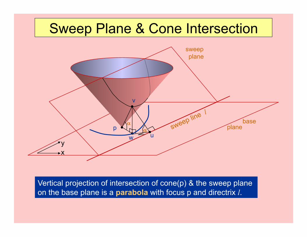
Sweep Plane & Cone Intersection

Vertical projection of intersection of cone(p) & the sweep plane on the base plane is a parabola with focus p and directrix l.

x y

p

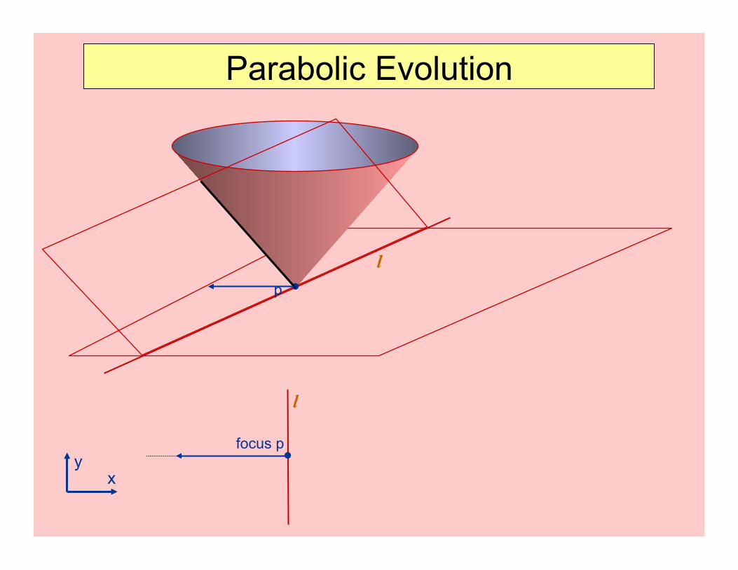
Parabolic Evolution

l

focus p

l

x y

p

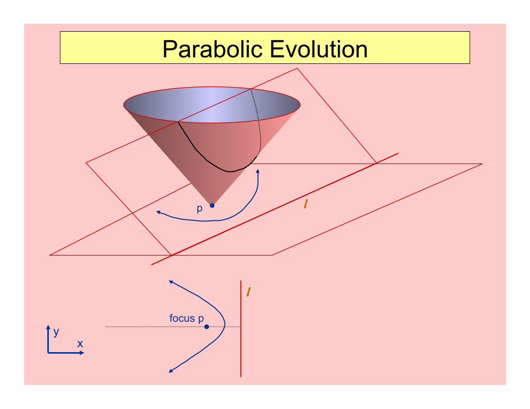
Parabolic Evolution

l

focus p

l

x y

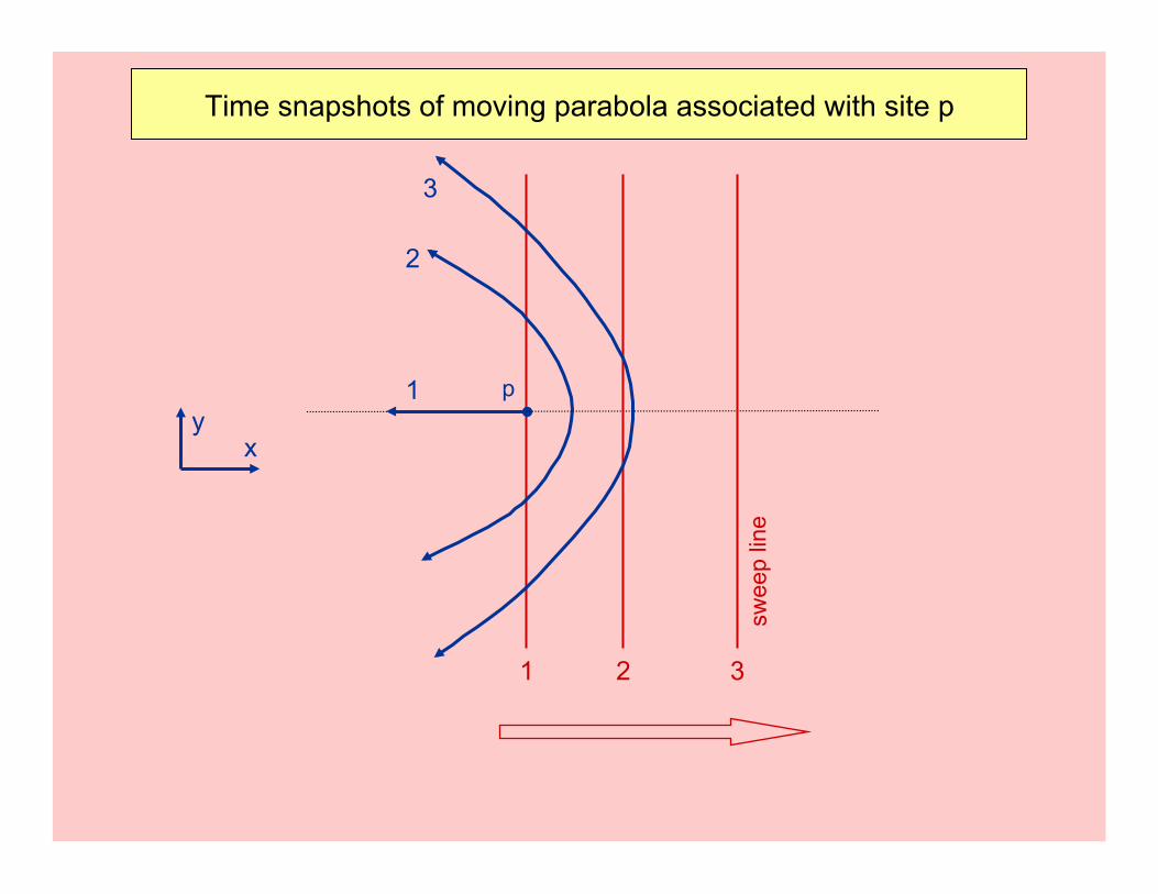
Time snapshots of moving parabola associated with site p

p

x y

1 2 3

1

2

3

swee

p lin

e

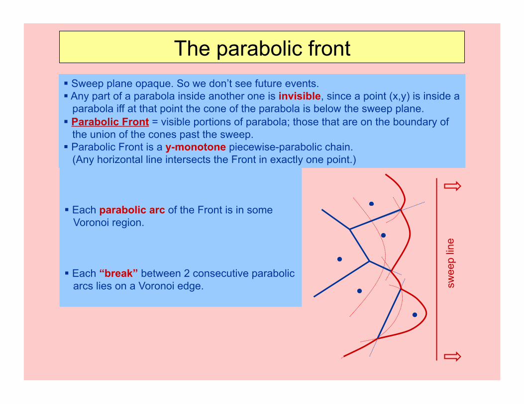
" Each parabolic arc of the Front is in some Voronoi region.

" Each break between 2 consecutive parabolic arcs lies on a Voronoi edge.

The parabolic front " Sweep plane opaque. So we dont see future events. " Any part of a parabola inside another one is invisible, since a point (x,y) is inside a parabola iff at that point the cone of the parabola is below the sweep plane. " Parabolic Front = visible portions of parabola; those that are on the boundary of the union of the cones past the sweep. " Parabolic Front is a y-monotone piecewise-parabolic chain. (Any horizontal line intersects the Front in exactly one point.)

swee

p lin

e

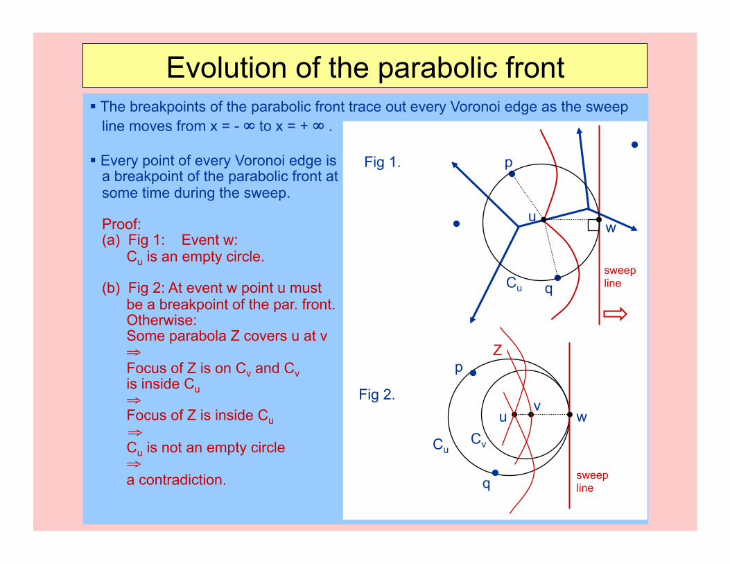
" The breakpoints of the parabolic front trace out every Voronoi edge as the sweep line moves from x = - , to x = + , .

" Every point of every Voronoi edge is a breakpoint of the parabolic front at some time during the sweep.

Proof: (a) Fig 1: Event w: Cu is an empty circle.

(b) Fig 2: At event w point u must be a breakpoint of the par. front. Otherwise: Some parabola Z covers u at v $ Focus of Z is on Cv and Cv is inside Cu $ Focus of Z is inside Cu $ Cu is not an empty circle $ a contradiction.

Evolution of the parabolic front

p

q

u w

Cu

Fig 1.

Fig 2. w u

v

Cu Cv

p

q

Z

sweep line

sweep line

" SITE EVENT: Insert into the Parabolic Front.

" CIRCLE EVENT: Delete from the Parabolic Front.

The Discrete Events

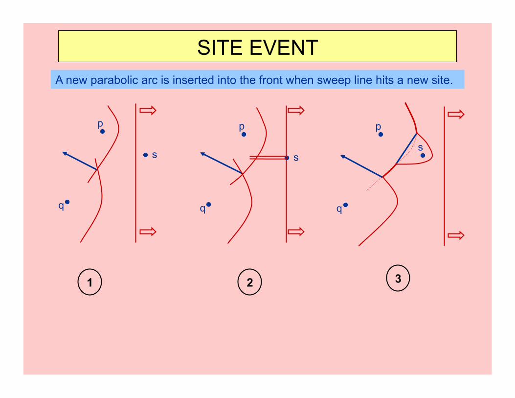
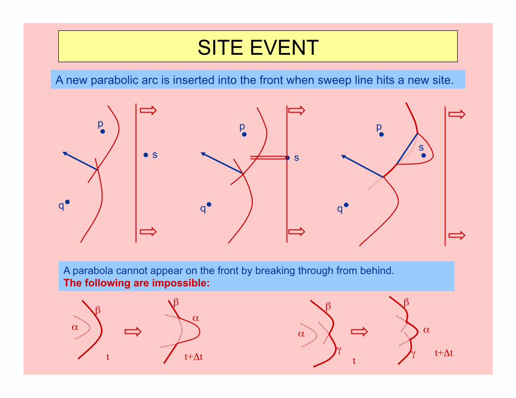
SITE EVENT A new parabolic arc is inserted into the front when sweep line hits a new site.

p

q

s

p

q

s

p

q

s

1 2 3

SITE EVENT

p

q

s

p

q

s

p

q

s

A parabola cannot appear on the front by breaking through from behind. The following are impossible:

*+

-+*+

-+

t t+.t

*+

-+

t t+.t /+

*+

-+

/+

A new parabolic arc is inserted into the front when sweep line hits a new site.

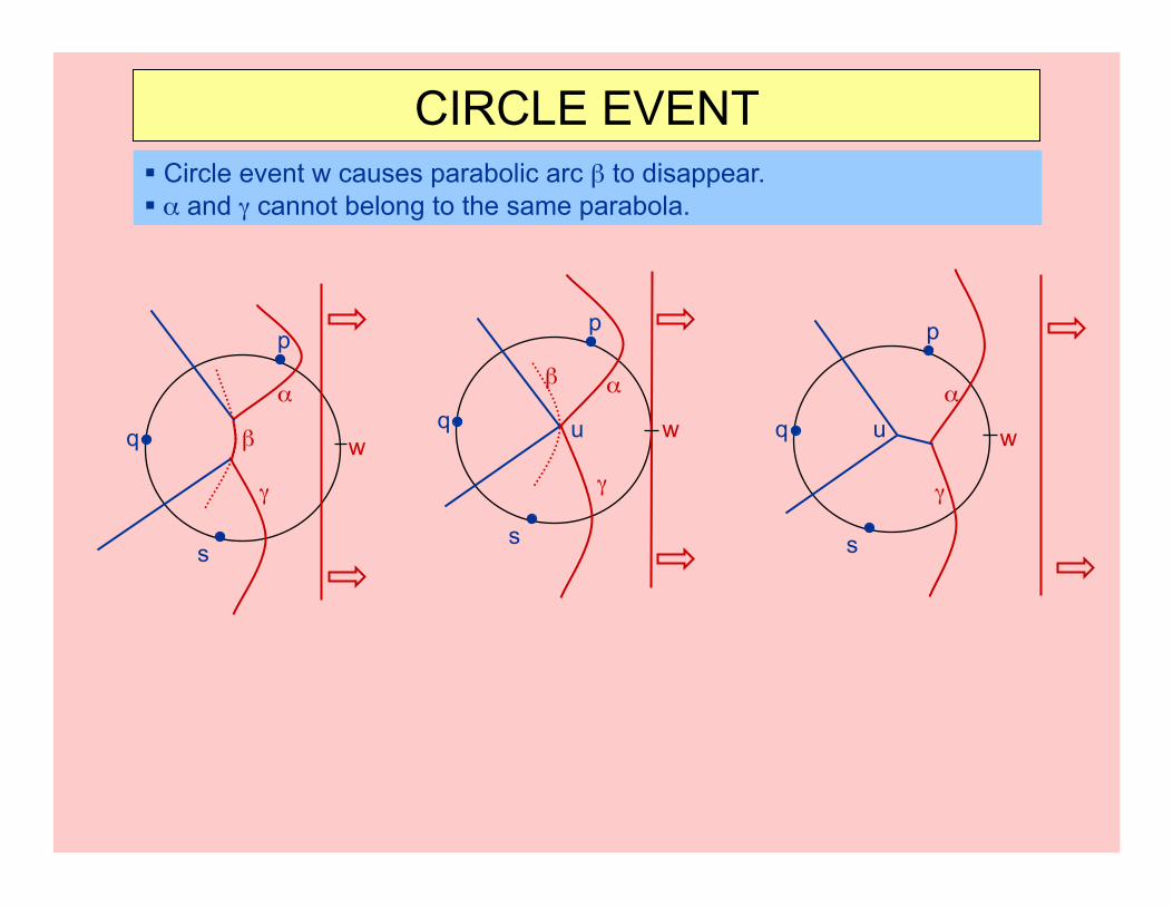
" Circle event w causes parabolic arc - to disappear. " * and / cannot belong to the same parabola.

CIRCLE EVENT

w

p

q

s

*+

/+

-+

u w

p

q

s

*+

/+

-+ w

p

q

s

*+

/+

u

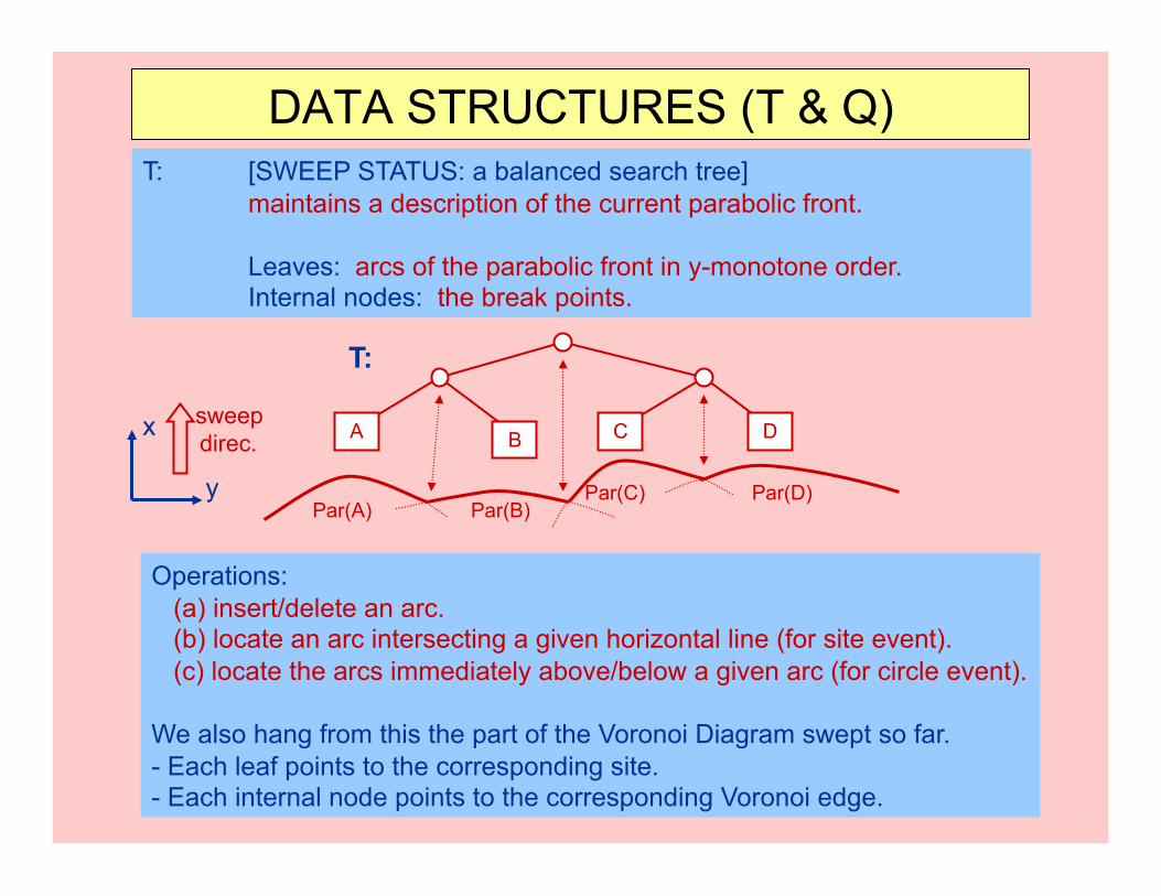
T: [SWEEP STATUS: a balanced search tree] maintains a description of the current parabolic front.

Leaves: arcs of the parabolic front in y-monotone order. Internal nodes: the break points.

DATA STRUCTURES (T & Q)

Operations: (a) insert/delete an arc. (b) locate an arc intersecting a given horizontal line (for site event). (c) locate the arcs immediately above/below a given arc (for circle event).

We also hang from this the part of the Voronoi Diagram swept so far. - Each leaf points to the corresponding site. - Each internal node points to the corresponding Voronoi edge.

x

y

sweep direc.

Par(A) Par(B) Par(C) Par(D)

A B C D

T:

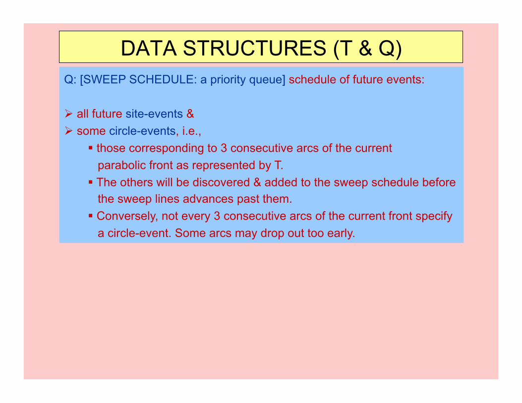
Q: [SWEEP SCHEDULE: a priority queue] schedule of future events:

# all future site-events & # some circle-events, i.e.,

" those corresponding to 3 consecutive arcs of the current parabolic front as represented by T. " The others will be discovered & added to the sweep schedule before the sweep lines advances past them. " Conversely, not every 3 consecutive arcs of the current front specify a circle-event. Some arcs may drop out too early.

DATA STRUCTURES (T & Q)

Event-driven simulation loop: At each iteration remove the next event (with min x-coordinate) from Q & simulate the effect of the sweep-line advancing past that event point.

Event Processing & Scheduling

Event-driven simulation loop: At each iteration remove the next event (with min x-coordinate) from Q & simulate the effect of the sweep-line advancing past that event point.

Event Processing & Scheduling

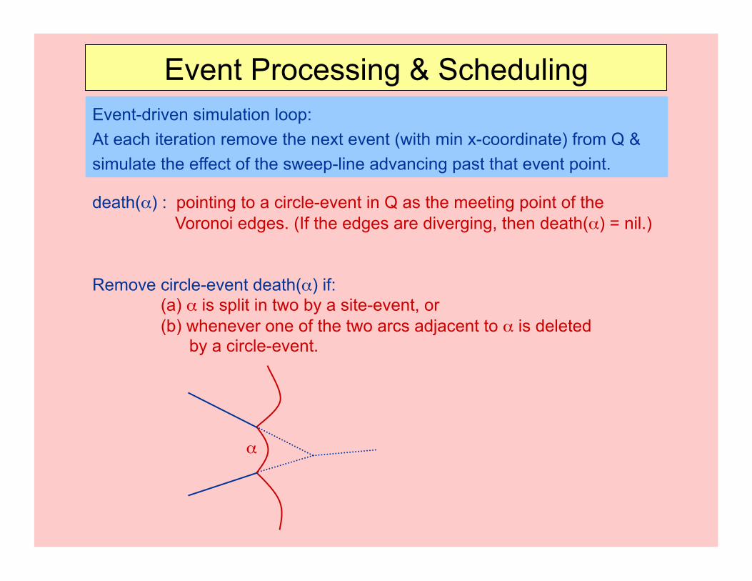
death(*) : pointing to a circle-event in Q as the meeting point of the Voronoi edges. (If the edges are diverging, then death(*) = nil.)

Remove circle-event death(*) if: (a) * is split in two by a site-event, or (b) whenever one of the two arcs adjacent to * is deleted by a circle-event.

*+

Event-driven simulation loop: At each iteration remove the next event (with min x-coordinate) from Q & simulate the effect of the sweep-line advancing past that event point.

Event Processing & Scheduling

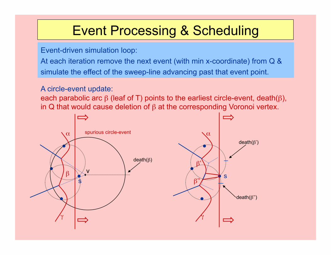
A circle-event update: each parabolic arc - (leaf of T) points to the earliest circle-event, death(-), in Q that would cause deletion of - at the corresponding Voronoi vertex.

death(-)

v s

*+

/+

-+

spurious circle-event

death(-)

s

*+

/+

-

-

death(-)

Event-driven simulation loop: At each iteration remove the next event (with min x-coordinate) from Q & simulate the effect of the sweep-line advancing past that event point.

Event Processing & Scheduling

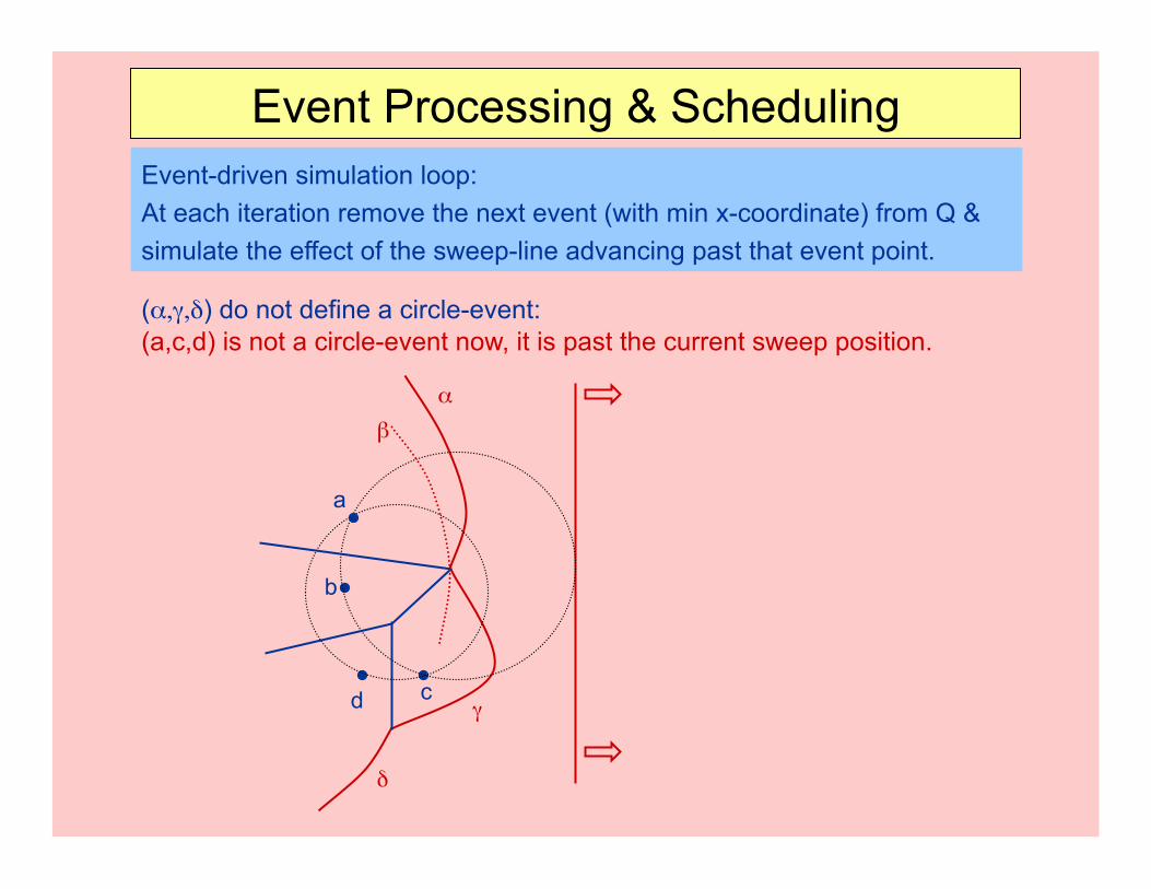
(*,/,0) do not define a circle-event: (a,c,d) is not a circle-event now, it is past the current sweep position.

a

b

*+

/+

-+

c d

0+

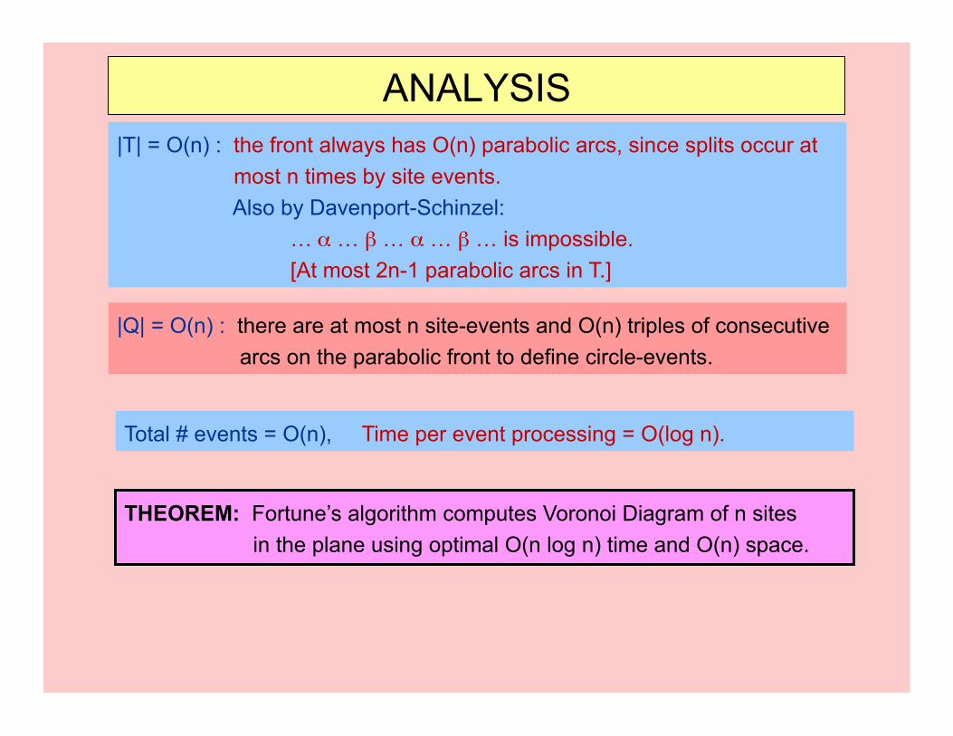
|T| = O(n) : the front always has O(n) parabolic arcs, since splits occur at most n times by site events. Also by Davenport-Schinzel: * - * - is impossible. [At most 2n-1 parabolic arcs in T.]

ANALYSIS

|Q| = O(n) : there are at most n site-events and O(n) triples of consecutive arcs on the parabolic front to define circle-events.

Total # events = O(n), Time per event processing = O(log n).

THEOREM: Fortunes algorithm computes Voronoi Diagram of n sites in the plane using optimal O(n log n) time and O(n) space.

Delaunay Triangulation

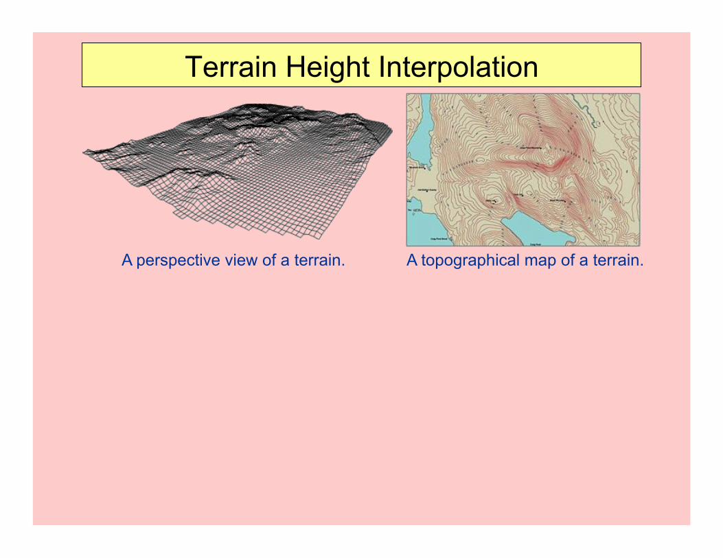
Terrain Height Interpolation

A perspective view of a terrain. A topographical map of a terrain.

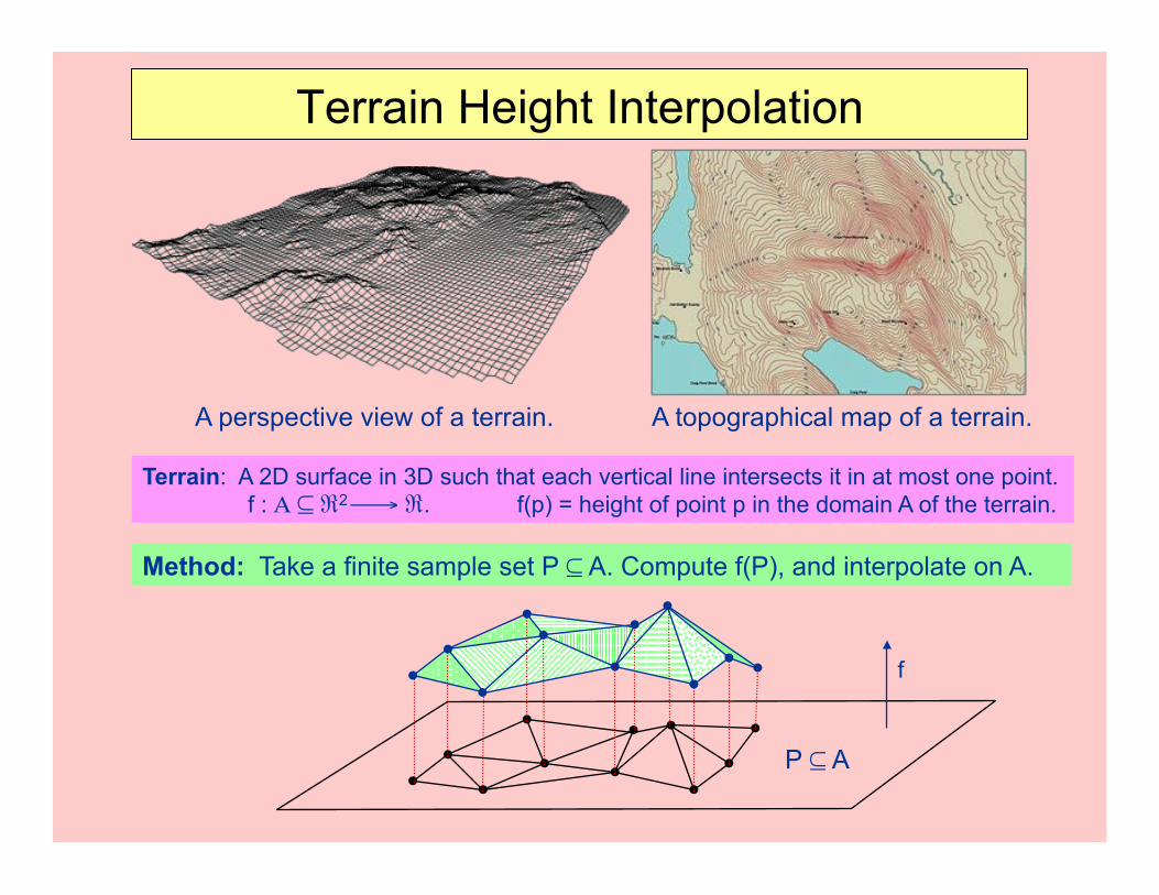
Terrain Height Interpolation

A perspective view of a terrain. A topographical map of a terrain.

Terrain: A 2D surface in 3D such that each vertical line intersects it in at most one point. f : 1 2 32 45 3. f(p) = height of point p in the domain A of the terrain.

Method: Take a finite sample set P 2 A. Compute f(P), and interpolate on A.

P 2 A

f

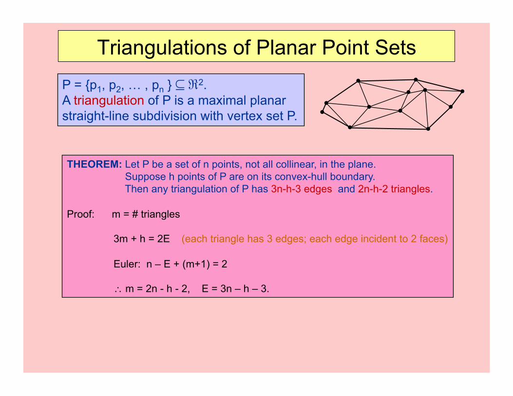
Triangulations of Planar Point Sets

P = {p1, p2, , pn } 2 32. A triangulation of P is a maximal planar straight-line subdivision with vertex set P.

THEOREM: Let P be a set of n points, not all collinear, in the plane. Suppose h points of P are on its convex-hull boundary. Then any triangulation of P has 3n-h-3 edges and 2n-h-2 triangles.

Proof: m = # triangles

3m + h = 2E (each triangle has 3 edges; each edge incident to 2 faces)

Euler: n E + (m+1) = 2

6 m = 2n - h - 2, E = 3n h 3.

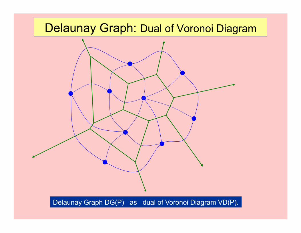
Delaunay Graph: Dual of Voronoi Diagram

Delaunay Graph DG(P) as dual of Voronoi Diagram VD(P).

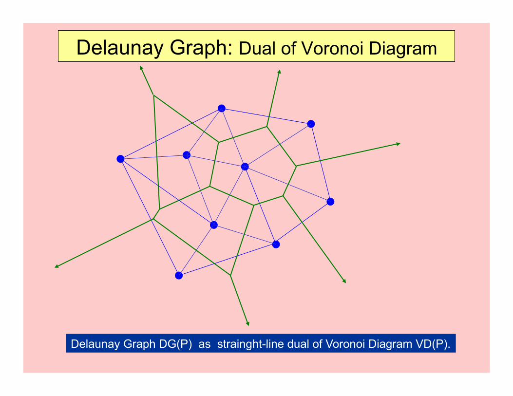
Delaunay Graph: Dual of Voronoi Diagram

Delaunay Graph DG(P) as strainght-line dual of Voronoi Diagram VD(P).

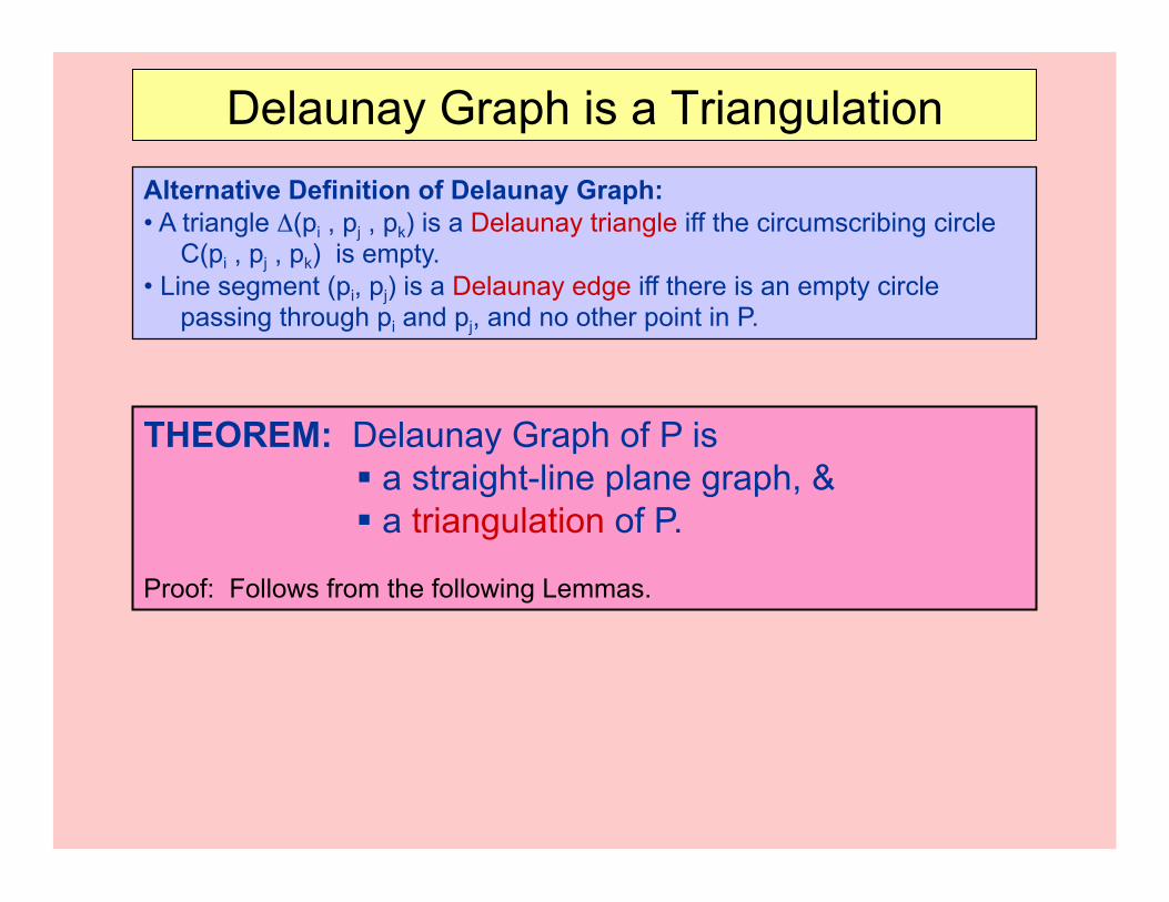
Delaunay Graph is a Triangulation

THEOREM: Delaunay Graph of P is " a straight-line plane graph, & " a triangulation of P.

Proof: Follows from the following Lemmas.

Alternative Definition of Delaunay Graph: A triangle .(pi , pj , pk) is a Delaunay triangle iff the circumscribing circle C(pi , pj , pk) is empty. Line segment (pi, pj) is a Delaunay edge iff there is an empty circle passing through pi and pj, and no other point in P.

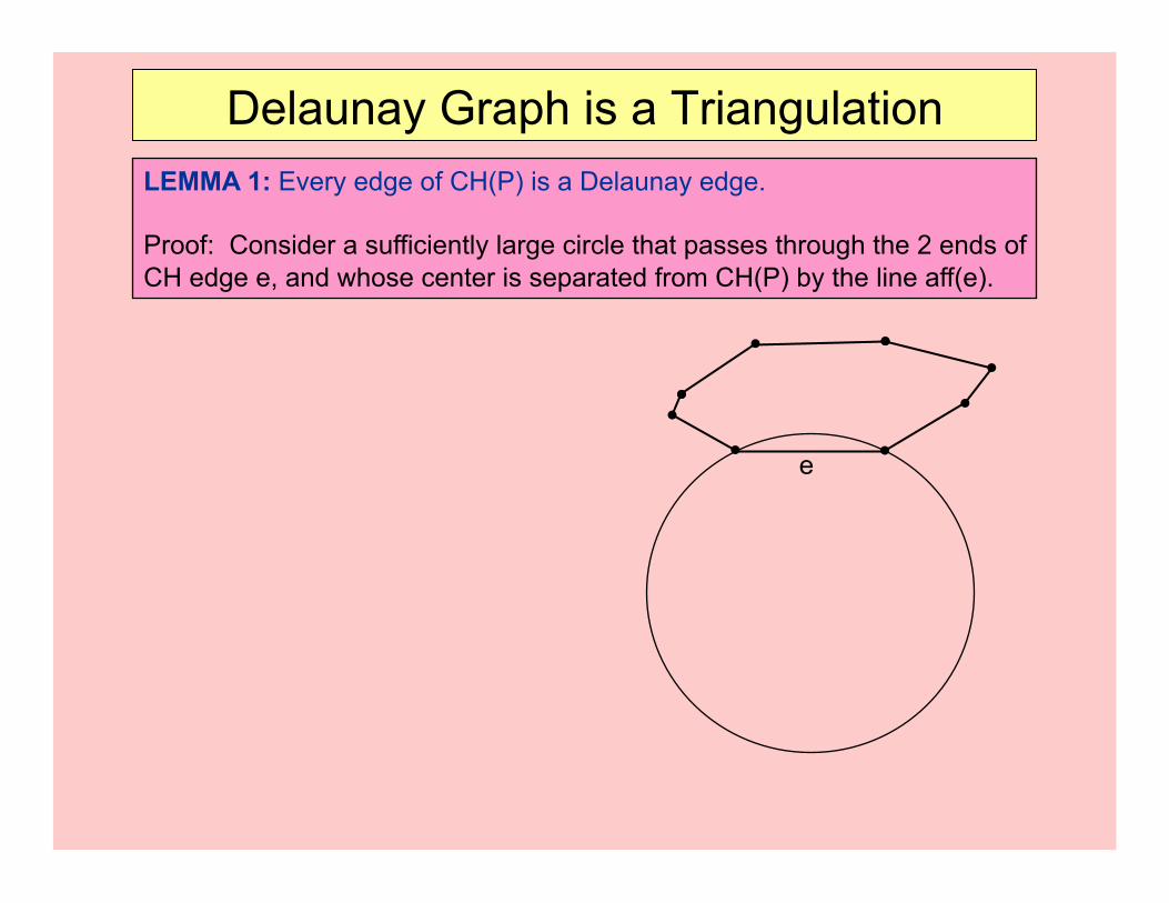
Delaunay Graph is a Triangulation LEMMA 1: Every edge of CH(P) is a Delaunay edge.

Proof: Consider a sufficiently large circle that passes through the 2 ends of CH edge e, and whose center is separated from CH(P) by the line aff(e).

e

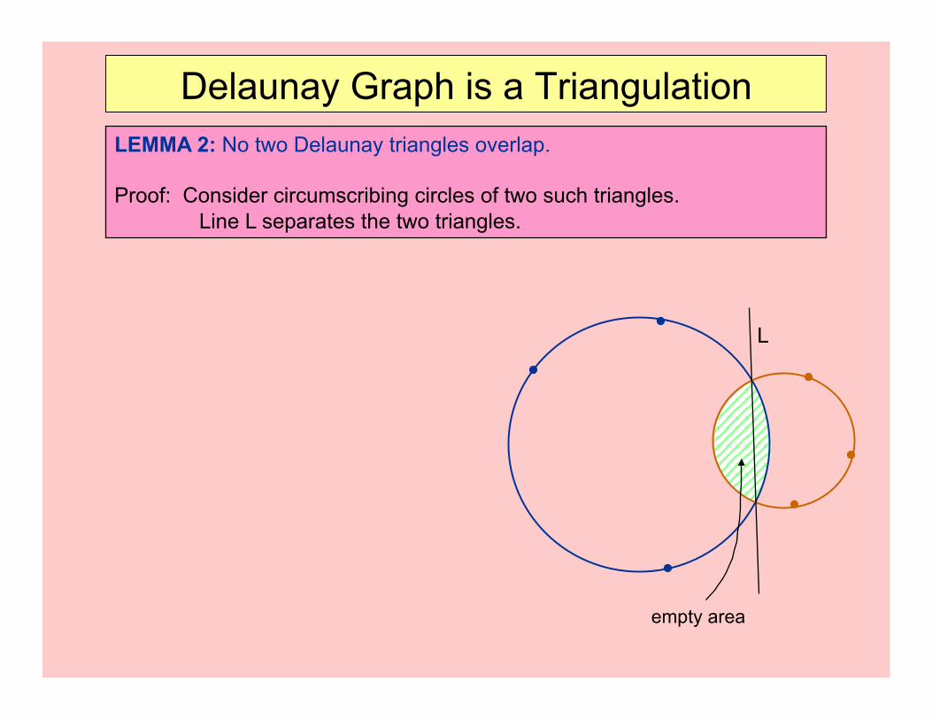
Delaunay Graph is a Triangulation LEMMA 2: No two Delaunay triangles overlap.

Proof: Consider circumscribing circles of two such triangles. Line L separates the two triangles.

L

empty area

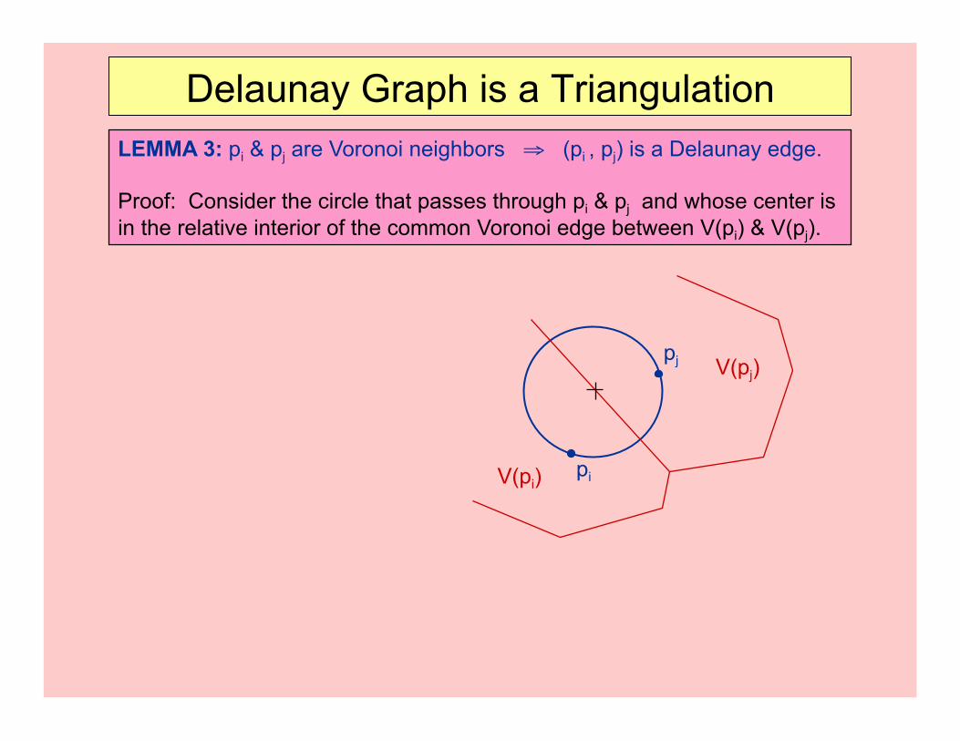
Delaunay Graph is a Triangulation LEMMA 3: pi & pj are Voronoi neighbors $ (pi , pj) is a Delaunay edge.

Proof: Consider the circle that passes through pi & pj and whose center is in the relative interior of the common Voronoi edge between V(pi) & V(pj).

V(pi)

V(pj)

pi

pj

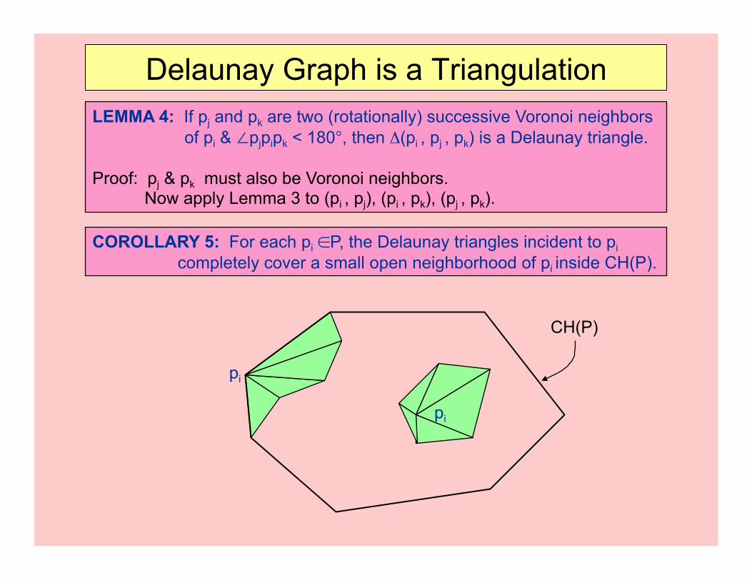
Delaunay Graph is a Triangulation LEMMA 4: If pj and pk are two (rotationally) successive Voronoi neighbors

of pi & 7pjpipk < 180, then .(pi , pj , pk) is a Delaunay triangle.

Proof: pj & pk must also be Voronoi neighbors. Now apply Lemma 3 to (pi , pj), (pi , pk), (pj , pk).

Delaunay Graph is a Triangulation LEMMA 4: If pj and pk are two (rotationally) successive Voronoi neighbors

of pi & 7pjpipk < 180, then .(pi , pj , pk) is a Delaunay triangle.

Proof: pj & pk must also be Voronoi neighbors. Now apply Lemma 3 to (pi , pj), (pi , pk), (pj , pk).

COROLLARY 5: For each pi 8P, the Delaunay triangles incident to pi completely cover a small open neighborhood of pi inside CH(P).

pi

pi

CH(P)

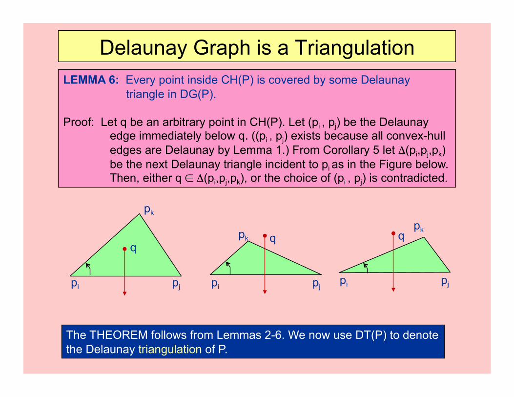
Delaunay Graph is a Triangulation LEMMA 6: Every point inside CH(P) is covered by some Delaunay

triangle in DG(P).

Proof: Let q be an arbitrary point in CH(P). Let (pi , pj) be the Delaunay edge immediately below q. ((pi , pj) exists because all convex-hull edges are Delaunay by Lemma 1.) From Corollary 5 let .(pi,pj,pk) be the next Delaunay triangle incident to pi as in the Figure below. Then, either q 8 .(pi,pj,pk), or the choice of (pi , pj) is contradicted.

pi pj

pk

q

pi pj

pk q

pi pj

pk q

The THEOREM follows from Lemmas 2-6. We now use DT(P) to denote the Delaunay triangulation of P.

Angles in Delaunay Triangulation

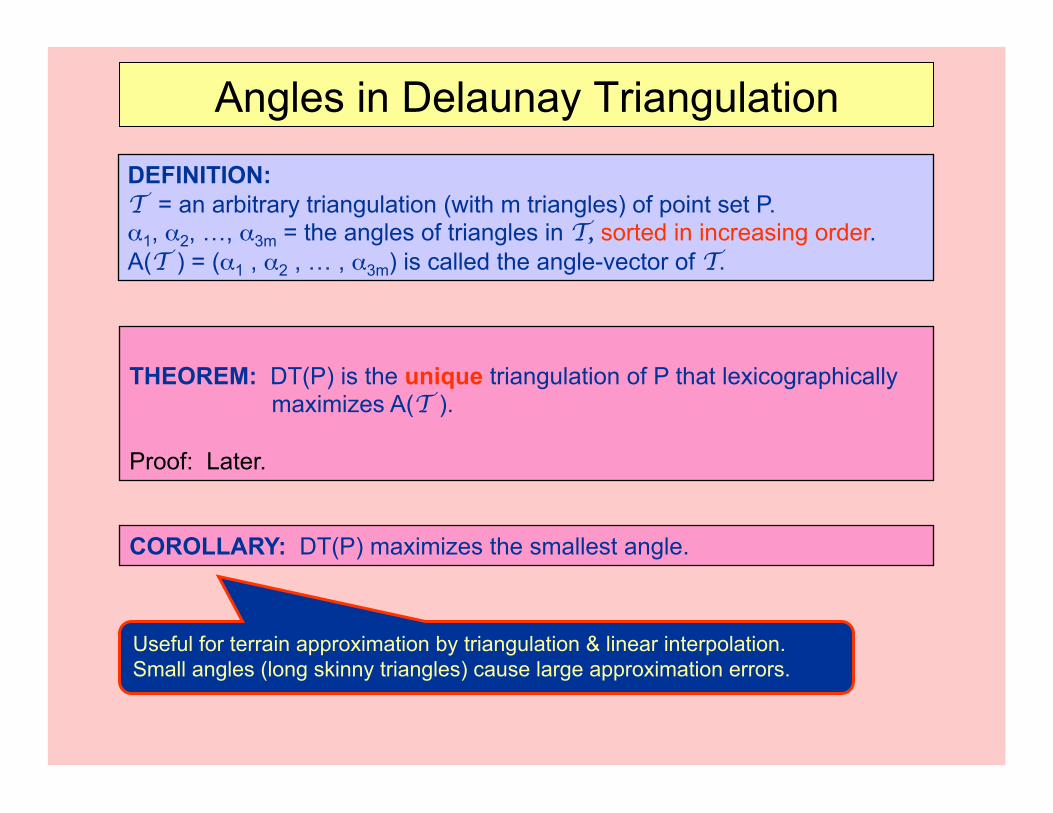
THEOREM: DT(P) is the unique triangulation of P that lexicographically maximizes A(T ).

Proof: Later.

DEFINITION: T = an arbitrary triangulation (with m triangles) of point set P. *1, *2, , *3m = the angles of triangles in T, sorted in increasing order. A(T ) = (*1 , *2 , , *3m) is called the angle-vector of T.

COROLLARY: DT(P) maximizes the smallest angle.

Useful for terrain approximation by triangulation & linear interpolation. Small angles (long skinny triangles) cause large approximation errors.

DT & VD via CH

K.Q. Brown [1979], Voronoi diagrams from convex hulls, IPL 223-228.

K.Q. Brown [1980], Geometric transforms for fast geometric algorithms, PhD. Thesis, CMU-CS-80-101.

Guibas, Stolfi [1987], Ruler, Compass and computer: The design and analysis of geometric algorithms, Proc. of the NATO Advanced Science Institute, series F, vol. 40: Theoretical Foundations of Computer Graphics and CAD, 111-165.

Guibas, Stolfi [1985], Primitives for the manipulation of general subdivisions and the computation of Voronoi diagrams, ACM Trans. Graphics 4(2), 74-123.

[Edelsbrunner87] pp: 302-306.

Aurenhammer [1987], Power diagrams: properties, algorithms, and applications, SIAM J. Computing 16, 78-96.

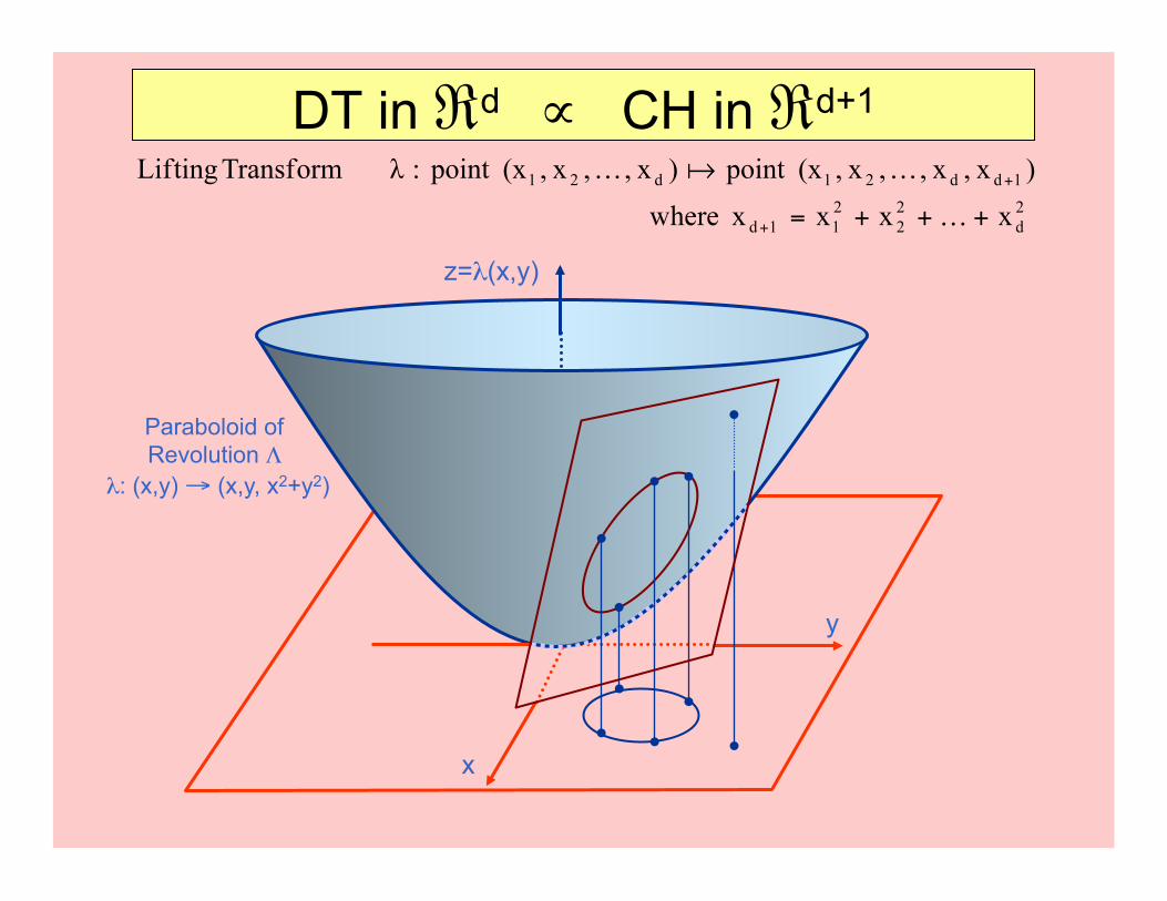
DT in 3d 9 CH in 3d+1

y

x

z=:(x,y)

Paraboloid of Revolution ;

:: (x,y) 5 (x,y, x2+y2)

SUMMARY:

Consider a plane < in 33 and the paraboloid of revolution ;.

(1) Projection of

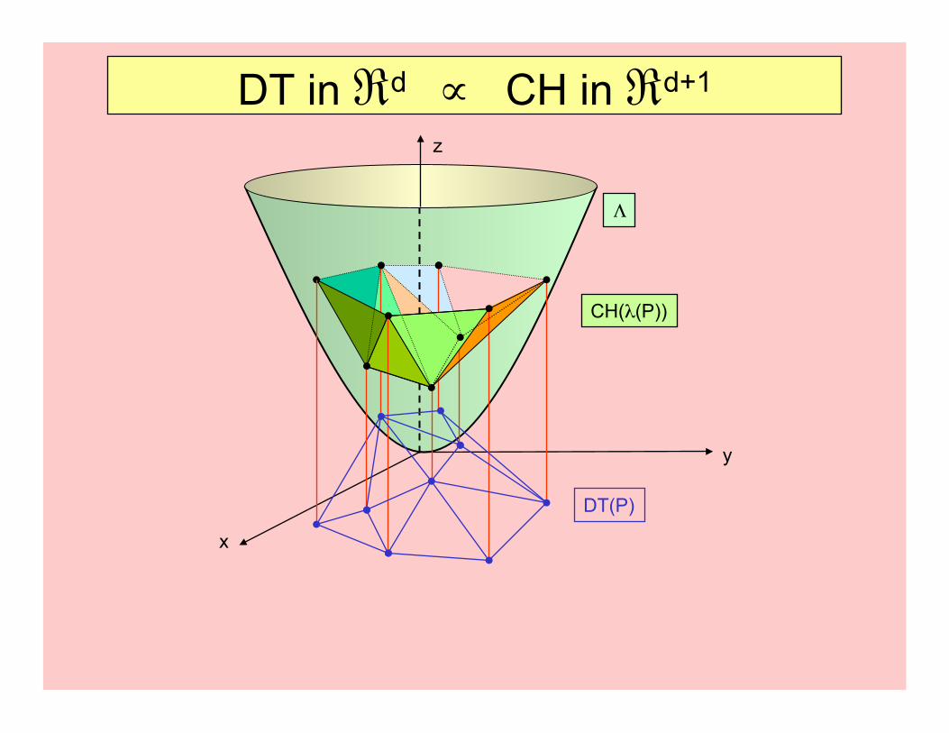
DT in 3d 9 CH in 3d+1

x

y

z

;

CH(:(P))

DT(P)

Generalizations & Applications

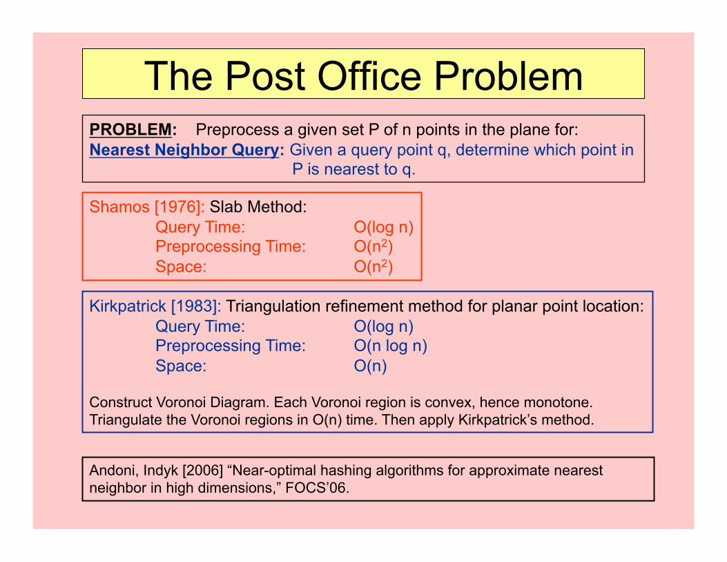
The Post Office Problem PROBLEM: Preprocess a given set P of n points in the plane for: Nearest Neighbor Query: Given a query point q, determine which point in

P is nearest to q.

Shamos [1976]: Slab Method: Query Time: O(log n) Preprocessing Time: O(n2) Space: O(n2)

Kirkpatrick [1983]: Triangulation refinement method for planar point location: Query Time: O(log n) Preprocessing Time: O(n log n) Space: O(n)

Construct Voronoi Diagram. Each Voronoi region is convex, hence monotone. Triangulate the Voronoi regions in O(n) time. Then apply Kirkpatricks method.

Andoni, Indyk [2006] Near-optimal hashing algorithms for approximate nearest neighbor in high dimensions, FOCS06.

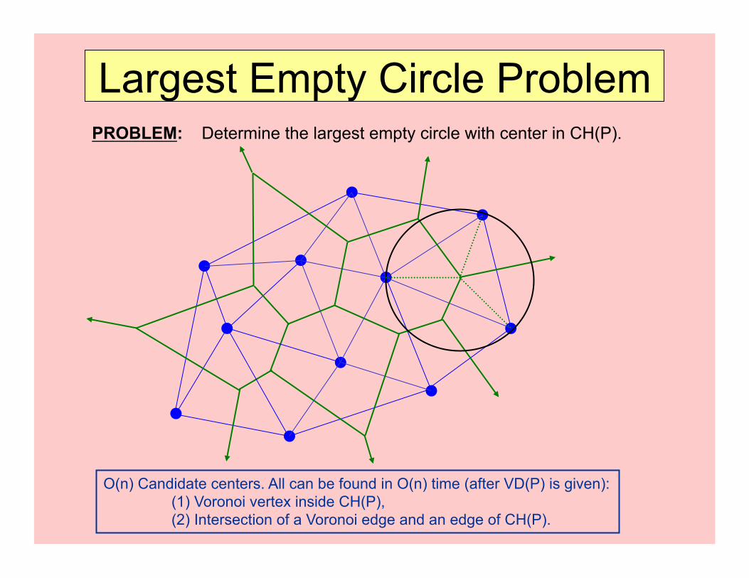
Largest Empty Circle Problem PROBLEM: Determine the largest empty circle with center in CH(P).

O(n) Candidate centers. All can be found in O(n) time (after VD(P) is given): (1) Voronoi vertex inside CH(P), (2) Intersection of a Voronoi edge and an edge of CH(P).

! Gabriel Graph ! Relative Neighborhood Graph ! Euclidean Minimum Spanning Tree ! Nearest Neighbor Graph

Subgraphs of Delaunay Triangulation

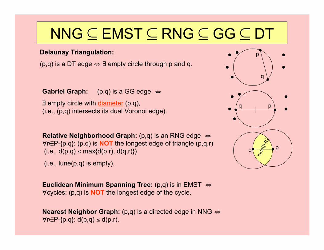
Nearest Neighbor Graph: (p,q) is a directed edge in NNG " >r8P-{p,q}: d(p,q) ! d(p,r).

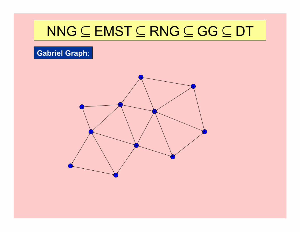
NNG 2 EMST 2 RNG 2 GG 2 DT p

q

Delaunay Triangulation:

(p,q) is a DT edge " % empty circle through p and q.

p q

Gabriel Graph: (p,q) is a GG edge "

% empty circle with diameter (p,q), (i.e., (p,q) intersects its dual Voronoi edge).

p q

Relative Neighborhood Graph: (p,q) is an RNG edge " >r8P-{p,q}: (p,q) is NOT the longest edge of triangle (p,q,r) (i.e., d(p,q) ! max{d(p,r), d(q,r)})

(i.e., lune(p,q) is empty).

Euclidean Minimum Spanning Tree: (p,q) is in EMST " >cycles: (p,q) is NOT the longest edge of the cycle.

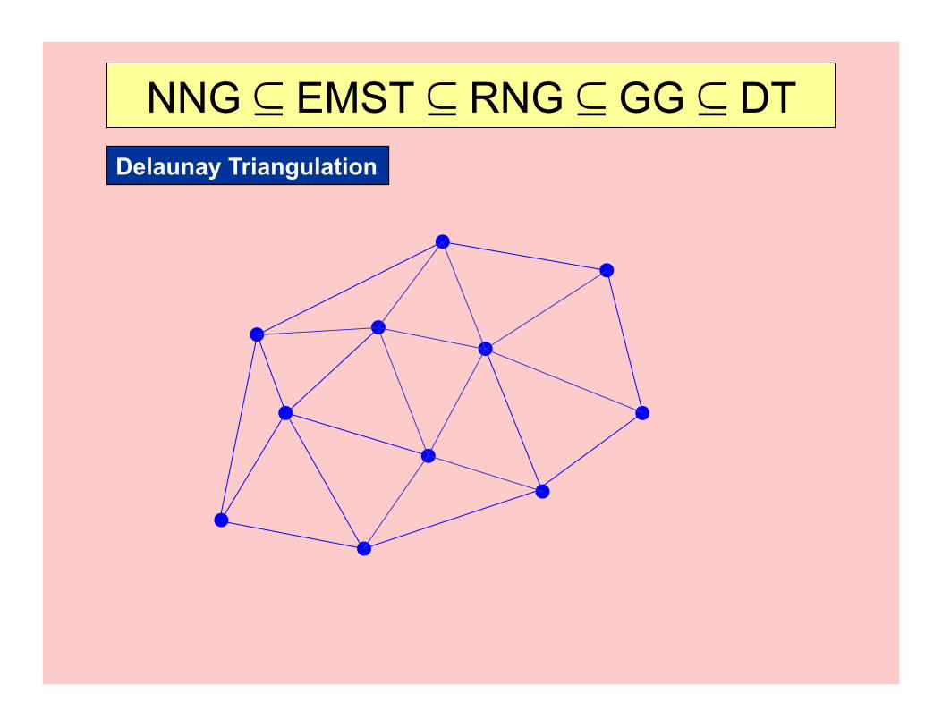
NNG 2 EMST 2 RNG 2 GG 2 DT Delaunay Triangulation

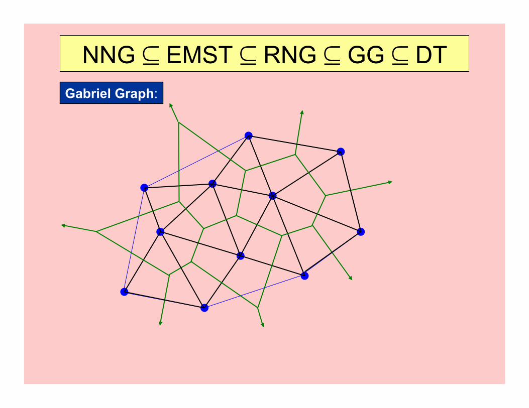
NNG 2 EMST 2 RNG 2 GG 2 DT Gabriel Graph:

NNG 2 EMST 2 RNG 2 GG 2 DT Gabriel Graph:

NNG 2 EMST 2 RNG 2 GG 2 DT Relative Neighborhood Graph:

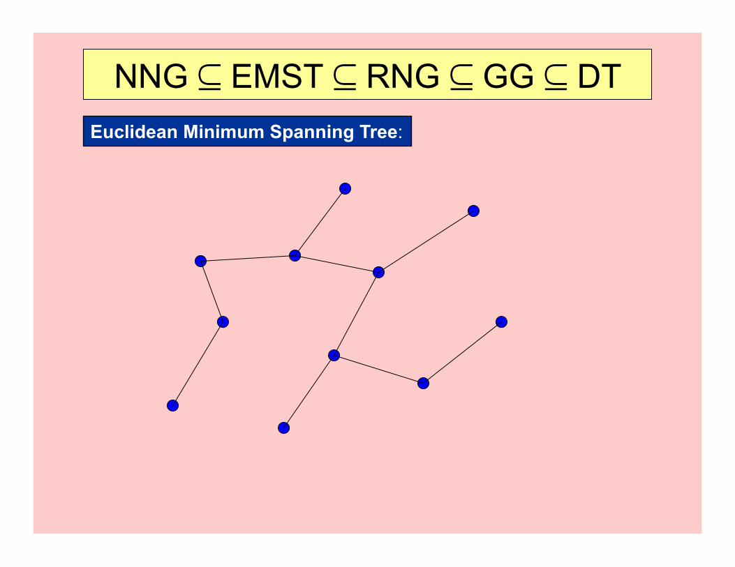
NNG 2 EMST 2 RNG 2 GG 2 DT Euclidean Minimum Spanning Tree:

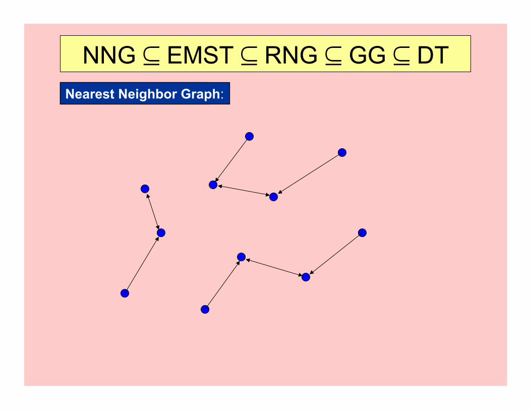
NNG 2 EMST 2 RNG 2 GG 2 DT Delaunay Triangulation Nearest Neighbor Graph:

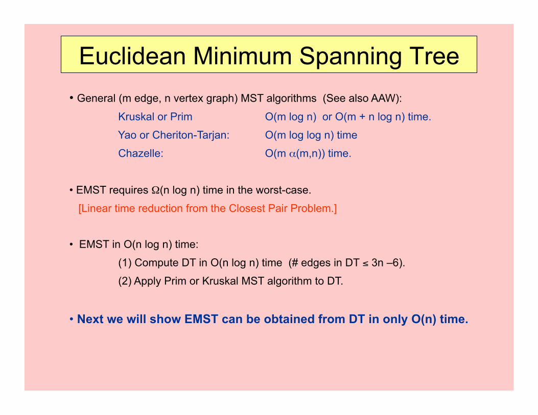
Euclidean Minimum Spanning Tree General (m edge, n vertex graph) MST algorithms (See also AAW):

Kruskal or Prim O(m log n) or O(m + n log n) time.

Yao or Cheriton-Tarjan: O(m log log n) time

Chazelle: O(m *(m,n)) time.

EMST requires ?(n log n) time in the worst-case. [Linear time reduction from the Closest Pair Problem.]

EMST in O(n log n) time: (1) Compute DT in O(n log n) time (# edges in DT ! 3n 6).

(2) Apply Prim or Kruskal MST algorithm to DT.

Next we will show EMST can be obtained from DT in only O(n) time.

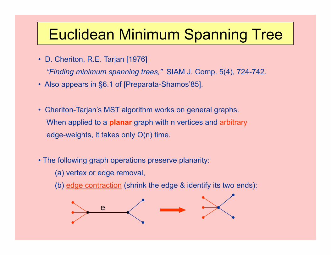
Euclidean Minimum Spanning Tree D. Cheriton, R.E. Tarjan [1976] Finding minimum spanning trees, SIAM J. Comp. 5(4), 724-742.

Also appears in 6.1 of [Preparata-Shamos85].

Cheriton-Tarjans MST algorithm works on general graphs. When applied to a planar graph with n vertices and arbitrary edge-weights, it takes only O(n) time.

The following graph operations preserve planarity: (a) vertex or edge removal,

(b) edge contraction (shrink the edge & identify its two ends):

e

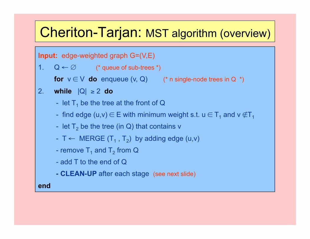
Cheriton-Tarjan: MST algorithm (overview) Input: edge-weighted graph G=(V,E) 1. Q & @ (* queue of sub-trees *)

for v 8 V do enqueue (v, Q) (* n single-node trees in Q *) 2. while |Q| A 2 do

- let T1 be the tree at the front of Q

- find edge (u,v) 8 E with minimum weight s.t. u 8 T1 and v BT1

- let T2 be the tree (in Q) that contains v

- T & MERGE (T1 , T2) by adding edge (u,v)

- remove T1 and T2 from Q

- add T to the end of Q

- CLEAN-UP after each stage (see next slide) end

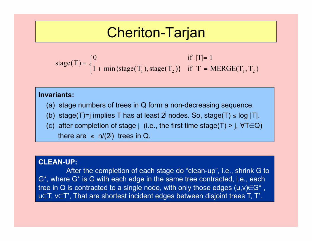
Cheriton-Tarjan

Invariants: (a) stage numbers of trees in Q form a non-decreasing sequence. (b) stage(T)=j implies T has at least 2j nodes. So, stage(T) ! log |T|. (c) after completion of stage j (i.e., the first time stage(T) > j, >T8Q) there are ! n/(2j) trees in Q.

CLEAN-UP: After the completion of each stage do clean-up, i.e., shrink G to

G*, where G* is G with each edge in the same tree contracted, i.e., each tree in Q is contracted to a single node, with only those edges (u,v)8G* , u8T, v8T, That are shortest incident edges between disjoint trees T, T.

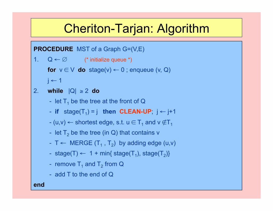
Cheriton-Tarjan: Algorithm PROCEDURE MST of a Graph G=(V,E) 1. Q & @ (* initialize queue *)

for v 8 V do stage(v) & 0 ; enqueue (v, Q) j & 1

2. while |Q| A 2 do - let T1 be the tree at the front of Q

- if stage(T1) = j then CLEAN-UP; j & j+1 - (u,v) & shortest edge, s.t. u 8 T1 and v BT1

- let T2 be the tree (in Q) that contains v

- T & MERGE (T1 , T2) by adding edge (u,v)

- stage(T) & 1 + min{ stage(T1), stage(T2)}

- remove T1 and T2 from Q

- add T to the end of Q

end

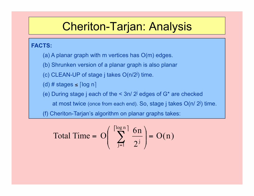
Cheriton-Tarjan: Analysis FACTS:

(a) A planar graph with m vertices has O(m) edges.

(b) Shrunken version of a planar graph is also planar

(c) CLEAN-UP of stage j takes O(n/2j) time.

(d) # stages ! Clog nD

(e) During stage j each of the < 3n/ 2j edges of G* are checked

at most twice (once from each end). So, stage j takes O(n/ 2j) time.

(f) Cheriton-Tarjans algorithm on planar graphs takes:

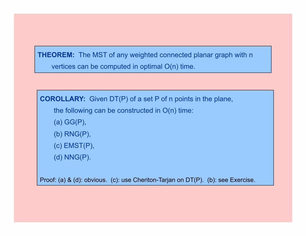
THEOREM: The MST of any weighted connected planar graph with n vertices can be computed in optimal O(n) time.

COROLLARY: Given DT(P) of a set P of n points in the plane, the following can be constructed in O(n) time:

(a) GG(P),

(b) RNG(P),

(c) EMST(P),

(d) NNG(P).

Proof: (a) & (d): obvious. (c): use Cheriton-Tarjan on DT(P). (b): see Exercise.

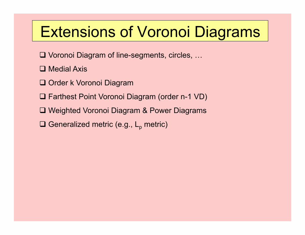
Extensions of Voronoi Diagrams ! Voronoi Diagram of line-segments, circles,

! Medial Axis

! Order k Voronoi Diagram

! Farthest Point Voronoi Diagram (order n-1 VD)

! Weighted Voronoi Diagram & Power Diagrams

! Generalized metric (e.g., Lp metric)

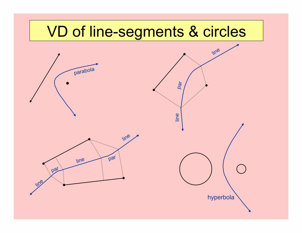
VD of line-segments & circles

parabola

par

line

par

hyperbola

Higher Order VD [PrS85] 6.3

[Ede87] 13.3-13.5

[ORo98] 6.6.

Aurenhammer [1987], Power diagrams: properties, algorithms, and applications, SIAM J. Computing 16, 78-96.

D.T. Lee [1982], On k-Nearest Neighbors Voronoi Diagram in the Plane, IEEE Trans. Computers, C-31, 478-487.

1

2

3

5

4 1,2

7

6 8

1,3

3,7

7,8

6,8

5,8

5,6 2,5

2,4

4,5

1,4 4,6

3,4 4,7

6,7

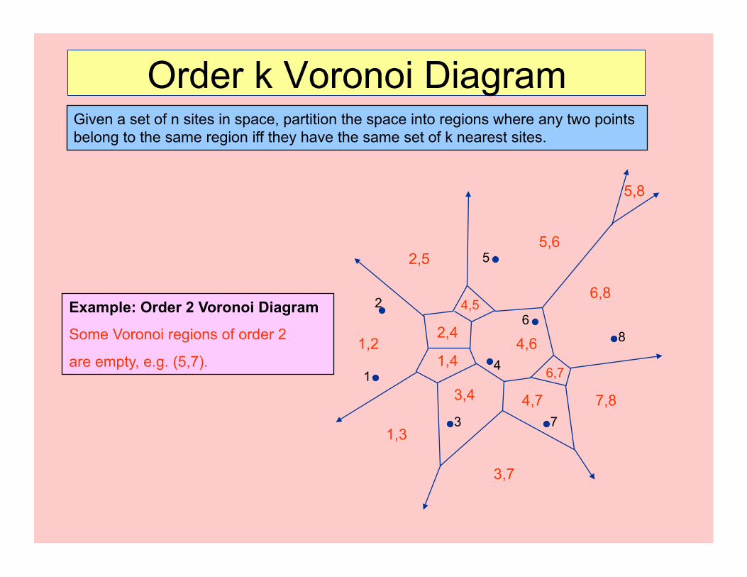
Example: Order 2 Voronoi Diagram

Some Voronoi regions of order 2

are empty, e.g. (5,7).

Order k Voronoi Diagram Given a set of n sites in space, partition the space into regions where any two points belong to the same region iff they have the same set of k nearest sites.

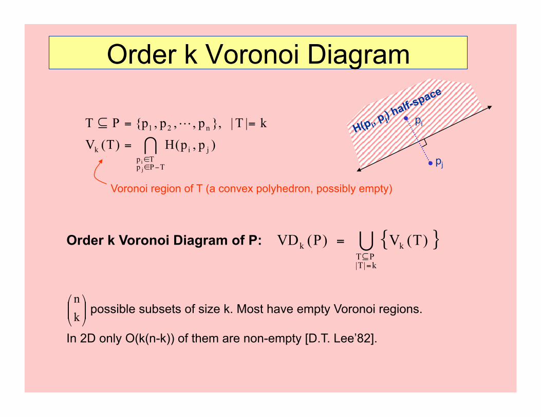
Order k Voronoi Diagram of P:

Order k Voronoi Diagram

Voronoi region of T (a convex polyhedron, possibly empty)

pi

pj

possible subsets of size k. Most have empty Voronoi regions.

In 2D only O(k(n-k)) of them are non-empty [D.T. Lee82].

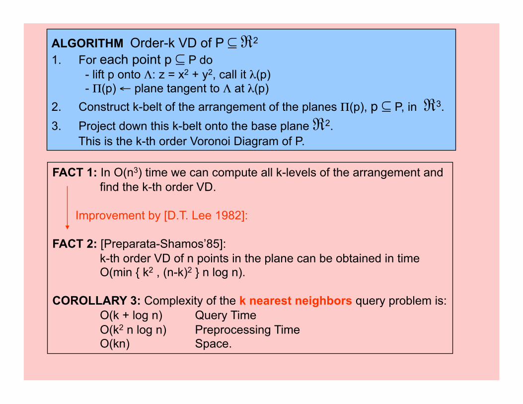
ALGORITHM Order-k VD of P 2 32 1. For each point p 2 P do

- lift p onto ;: z = x2 + y2, call it :(p) -