Detached-Eddy Simulations of the Flow Structures Underneath aFrancis Turbine Runner

Carl-Anthony Beaubien1, Guy Dumas1, and Guillaume Boutet-Blais2

1 Laboratoire de Mécanique des Fluides NumériqueDepartment of Mechanical Engineering, Laval University, Québec, QC, G1V 0A6, Canada

2 Alstom Power & Transport Canada Inc1350 chemin St-Roch, Sorel-Tracy, QC, J3R 5P9, Canada

Email: carl-anthony.beaubien.1@ulaval.ca

ABSTRACT

The effect of the vortical flow structures ejected by a Fran-cis turbine runner on the flow downstream, in the draft tube,is evaluated in this investigation. Calculations are performedwith the commercial code ANSYS CFX 13.0 and with the tur-bulence modeling approach DES-SST as proposed by Menterand Kuntz [8].

First, the grid and time step requirements are assessed on asimplified geometry, which includes the draft tube cone anda straight extension. It is shown that a very fine mesh andtime step resolution are necessary to capture adequately theflow structures without their premature diffusion underneaththe inlet plane, even if the modeled turbulence at the inlet isneglected.

Then, two draft tube flow simulations are compared. The firstone includes the unsteady flow structures ejected by the run-ner and the second one has steady circumferentially averagedvelocity profiles imposed at the inlet plane. At the operat-ing point investigated, the flow topology and the performanceof the diffuser are found to be only slightly affected by thecoherent flow structures expelled by the turbine runner.

1 INTRODUCTION

The flow in the draft tube of hydraulic turbines is particularlycomplex and can present a significant challenge for Compu-tational Fluid Dynamics (CFD). For turbine refurbishment,the existing draft tube may not be optimal, leading to flowseparation and significant efficiency losses. In such cases,performance predictions may be unreliable. Furthermore, theadaptation of a new runner design to the already existing drafttube can be a difficult task if draft tube predictions providedby CFD are inaccurate. Main components of the turbine areshown on Figure 1.

One suspects that some form of vortex breakdown and/or flow

Draft Tube

Spiral Casing

Runner

Draft TubeCone

Stay Vanes & Guide Vanes

Figure 1: Components of a Francis hydraulic turbine.

separation may occur in the adverse pressure gradient inter-nal flow of the draft tube. Such features are particularly dif-ficult to predict with turbulence modeling methods which areused to solve the Reynolds Averaged Navier-Stokes (RANS)equations. Indeed, it is widely known that these models pro-duce much less reliable results in flows where there is strongstreamlines curvature, flow rotation or boundary layer sepa-ration [10] [11].

Therefore, Detached-Eddy Simulation (DES) is tested in thiswork, in order to make an attempt at improving the predic-tion of those phenomena in the draft tube. However, this tur-bulence modeling approach, which implies simulating largeturbulent eddies outside the boundary layers, requires inletboundary conditions which are consistent with the method.Large unsteady vortical structures ejected by the runner couldbe needed at the draft tube computational domain inlet planesituated below the turbine runner. It is not the case in RANSsimulations where a steady-state solution is produced. Thevelocity field at the inlet plane is then time averaged.

1

Gagnon et al. [3] recently performed experimental measure-ments of the flow underneath a propeller turbine. These au-thors attribute the large scale unsteady fluctuations in the ve-locity fields and associated vortical flow structures to two dis-tinct phenomena. The first one is the velocity gradient be-tween the runner blades and the second is the wake behindthe trailing edge created by the boundary layers leaving theblades.

In this work, the effect of inlet vortical flow structures on drafttube performance is assessed.

2 METHODOLOGY

Commercial software ANSYS CFX 13.0 is used to solve theNavier-Stokes equations. For an incompressible flow withuniform viscosity, they take the following form:

∂ui

∂xi= 0, (1)

∂ui

∂t+u j

∂ui

∂x j=−1

ρ

∂p∂xi

+ν∂2ui

∂x j∂x j, (2)

where ui is the velocity vector, p the static pressure, ν thekinematic viscosity, and ρ the density.

2.1 Turbulence Modeling

The convective term u j∂ui∂x j

in the Navier-Stokes equationsis responsible for turbulence which is characterized by flowstructures of various scales. Unfortunately, at the Reynoldsnumber of the studied flow (≈ 2.5×106 based on the inlet di-ameter of the draft tube), it is too costly to resolve the smallestturbulent flow structures. Therefore, a turbulence modelingapproach needs to be used.

In the present investigation, the turbulence modeling ap-proach employed is DES-SST, as proposed by Menter andKuntz [8]. Near the wall, in the boundary layers, a RANSapproach is used. The Reynolds decomposition is thereforeapplied on the Navier-Stokes equations, which gives :

∂Ui

∂xi= 0, (3)

∂Ui

∂t+U j

∂Ui

∂x j=−1

ρ

∂P∂xi

+∂

∂x j

(ν

∂Ui

∂x j+u′ju

′i

), (4)

where Ui is the ensemble averaged mean velocity vector, u′i isthe fluctuating part of the fluid velocity vector (ui = Ui + u′i)and P is the mean pressure. The term u′ju

′i is the Reynolds

stress tensor which represents the time-averaged rate of mo-mentum transfer due to turbulence.

Outside the boundary layers, a Large-Eddy Simulation (LES)approach is rather employed which enables the simulation oflarge scale turbulent structures. In this flow region, a spatialfilter is imposed on the Navier-Stokes equations, which leadsto :

∂Ui

∂xi= 0, (5)

∂Ui

∂t+U j

∂Ui

∂x j=−1

ρ

∂P∂xi

+∂

∂x j

(ν

∂Ui

∂x j+ τ

sgsi j

), (6)

where Ui is the filtered velocity, P the filtered static pressureand τ

sgsi j the subgrid-scale Reynolds stress tensor. The latter

represents the rate of momentum transfer generated by turbu-lent motions whose size is inferior to the size of the spatialfilter.

If the length scale of the largest turbulent structures lt isgreater than the size of the grid cells ∆, they are resolved andconsequently, the LES approach is used. In the opposite situ-ation, where lt < ∆, the RANS approach is used.

The similarity between the RANS and LES equations fa-cilitates the transition between the two turbulence modelingmethods. Both the Reynolds stress tensor and the subgrid-scale Reynolds stress tensor are computed through Menter’sSST model, which blends the two-equation models k-ε andk-ω [7]. To only model subgrid-scale turbulence in the LESregion, the modeled turbulence length scale is limited throughthe rate of dissipation of the turbulent energy ε [9]. Indeed,

ε = β∗ k ω FDES, (7)

FDES = max(

ltCDES∆

(1−FSST ) , 1), (8)

lt =

√k

β∗ω, (9)

where β∗ is a constant of the SST model (β∗ = 0.09), k isthe modeled turbulent kinetic energy, ω is the modeled tur-bulence specific dissipation rate and CDES is a constant equalto 0.61. FSST can be equal to 0, F1, or F2. F1 and F2 referto the SST blending functions described in [7]. In our case,FSST = F1. This is used to insure that the RANS approachis employed in the boundary layers, even if lt is slightlylarger than the grid size. This is to protect the boundary lay-ers against the "Grid-Induced Separation" phenomenon dis-cussed by Spalart [11]. B.-Vincent [1] showed that for thekind of flow considered in this study, DES formulations pro-tecting the boundary layer produce far better results.

2

2.2 Numerics

The solver uses an element based finite-volume method [4].The pressure and diffusive terms are discretized with finite-element shape functions which are linear in term of paramet-ric coordinates [4].

In the LES region of the domain, the convective term is alsodiscretized with shape functions. Since a linear interpolationis done in the element, this method corresponds to a CentralDifference Scheme (CDS). However, in the boundary layers,where a RANS turbulence modeling approach is used, ANSYSCFX’s "High Resolution" scheme is preferred. This schemecorresponds to a first order upwind differencing with a secondorder correction that varies in the domain, in order to be asclose as possible to a formal second-order-accurate schemebut without introducing non-physical oscillations.

The transient term is discretized using the second order back-ward Euler scheme.

Finally, the solver is a coupled one in which conservation ofmass is treated in the same way as conservation of momen-tum.

2.3 Boundary Conditions

A no-slip wall condition is applied to all solid boundaries ofthe domain. At the outlet, an average reference pressure isset. At the inlet plane, velocity profiles and turbulence char-acteristics are imposed. They were obtained by a RANS sim-ulation of one guide vane and one runner blade passage. Theobtained velocity field was then copied over all the inlet planecircumference and was put in rotation at the runner rotationspeed Ω. This strategy is illustrated on Figure 2. For somedraft tube simulations where an axisymmetric condition wasdesired, the velocity fields were circumferentially averagedinstead.

As for the inlet modeled turbulence, it was chosen to be ne-

glected outside the boundary layers, in the LES region. In-deed, since the object of this work is to assess the effect ofthe large scale flow structures ejected by the runner on thedraft tube behavior, it is wanted to minimize their diffusion,even if it may be in a exaggerated fashion. Therefore, if theireffect on the flow downstream is not perceptible, too impor-tant artificial diffusion from the turbulence model could notbe held responsible. In order to identify the boundary layerswhere the turbulence model quantities from the RANS simu-lation have to remain untouched, a similar approach from theone proposed by Spalart et al. [12] for DDES is used. First,the squared ratio of the modeled turbulent length scale to thewall distance is computed:

rd ≡νt +ν√

Ui, jUi, j κ2 d2. (10)

The velocity gradient tensor is Ui, j, κ is the Kármán constantand d is the distance to the closest wall. The parameter rd istherefore equal to unity in the logarithmic region and gradu-ally falls towards 0 as it gets further away from the wall. It isthen injected into the following equation :

fd ≡ 1− tanh([8rd ]3). (11)

The parameter fd is then equal to 1 in the LES region wherethe ratio of the modeled turbulence length scale to the walldistance is a lot smaller then unity. Everywhere else, fd isnull.

As discussed previously, it was chosen in this work to ne-glect the modeled part of the turbulent spectrum in the LESregion. Therefore, small values of νt/ν = 0.1 and I = 0.1%are imposed in the LES region of the inlet plane. To do so,the turbulent kinematic viscosity νt and turbulent intensity Iobtained from the RANS simulations of the upstream compo-nents, designated by the subscript RANS, are adjusted with thefollowing formulas:

Steady physical fieldsat the runner outlet

Copy of thephyhsical fields on

the inletplane whole

circumference

Imposition of thephysical fileds at

the draft tube inlet

Figure 2: Strategy used to impose the boundary conditions at the inlet of the draft tube.

3

νt = (νt)RANS (1− fd)+0.1ν fd , (12)I = IRANS (1− fd)+0.001 fd . (13)

The effect of this operation can be visualized on Figure 3.

Figure 3: Ratio of νt/ν and turbulent intensity a) from theRANS simulation of the upstream components and b) afterthe attenuation of the modeled turbulent quantities in the LESregion.

2.4 Grid Resolution

The flow structures ejected by the runner have small dimen-sions and rotate at a high velocity. Furthermore, many au-thors, such as Mauri [5], Cervantes et al. [2] and B.-Vincent[1], observed a rapid diffusion of these structures underneaththe inlet plane of the draft tube. It is suspected that a toocoarse spatial and time resolution may be the cause.

In order to establish the meshing and time step requirementsto capture adequately the vortical flow structures at the inletof the draft tube, simulations have been performed on a sim-plified geometry. It includes the draft tube cone and a straightextension which has the same length as the cone.

Five grids were tested. The number of nodes varied between2 and 15 millions. The time step corresponds to 0.5 of rota-tion of the runner. However, time discretization will be dis-cussed separately in the next section. For each mesh tested,the evolution of the vortical structures ejected by the runner

is shown on Figure 4. They are visualized with the q-criterionq = 1

2 (||Ri j||2−|||Si j||2) where Ri j is the rotation tensor andSi j is the strain-rate tensor. As shown, it is clear that the gridresolution has a strong effect on their propagation in the drafttube.

Furthermore, one can observe these large coherentanisotropic structures through the off-diagonal compo-nents of the Reynolds stress tensor. Figure 5 shows theReynolds stress tensor component < u′

θu′z > as a function

of the radial position on the inlet plane. It is compared tothe experimental measurements of Tridon et al. [14], whomeasured the axial and tangential velocity by LDV 0.13Dunder the runner at a similar operating point. D refers tothe runner diameter. The velocity profiles and fluctuationswere measured on three diameters and then averaged togive a profile on a single radius. Further details on theirexperimental methodology can also be found in [13].

Once again, the effect of the grid resolution is clearly visi-ble. The finest mesh, which counts nearly 15 M nodes is inreasonable agreement with the experimental data, especiallywhen it comes to the amplitude of the fluctuations. However,the slightly coarser mesh, which contains nearly 12 M nodesseems to be a good compromise between computational costand precision. It is felt that the effect of the large scale struc-tures under the runner should be well captured with this mesh.Therefore, this grid resolution will be transposed to the com-plete draft tube and used for further investigations.

2.5 Time Discretization

A similar approach is used to evaluate the necessary time stepresolution to adequately capture the vortical structures ejectedby the runner. Four time step resolutions are tested in thesimplified geometry. They correspond to 0.25, 0.5, 0.75

and 1 of rotation of the runner. The equivalent normalizedtime steps are shown in Table 1.

Table 1: Time steps tested in terms of runner rotation an-gle and normalized by the axial average velocity and runnerdiameter.

∆ ∆t∗ = 4Q∆tπD3

0.25 0.75×10−3

0.5 1.50×10−3

0.75 2.24×10−3

1 2.99×10−3

All simulations here were performed with the mesh contain-ing 11.7 M nodes. First, the vortical structures are shown withthe q-criterion on Figure 6. As for the the grid resolution, thetime step has a strong influence on the way the flow structures

4

Figure 4: Turbulent structures shown with the q-criterion for different meshes and ∆t∗ = 1.5×10−3 (q = 1500 s−2).

[13]

Figure 5: Circumferential average of Reynolds stress< u′

θu′z > as a function of the radial position 0.13D under

the runner. The time step corresponds to 0.5 of rotation ofthe runner (∆t∗ = 1.5×10−3).

propagate downstream.

This can also be felt when observing the Reynolds stresstensor component < u′

θu′z > in Figure 7. The amplitude of

the fluctuations are reduced with the two coarser time steps.However, the difference between the two finer time steps, of0.5 and 0.25, is very subtle. Therefore, a time step of 0.5

of rotation of the runner will be used for the simulation of thecomplete draft tube.

3 RESULTS

The necessary grid resolution, once transposed to the com-plete draft tube, generated a grid with nearly 31 M nodes.The quality criteria of the mesh are shown in Table 2.

In order to evaluate the effect of the vortical structures ejected

Table 2: Quality criteria of the draft tube mesh.

Min. Angle > 33.5

Determinant > 0.65Aspect Ratio < 1500

Expansion factor < 2.5

by the runner on the flow in the draft tube, two simulationshave been performed. The first one includes the structures atthe inlet, while for the second one, steady axisymmetric ve-locity profiles are imposed. In both cases, modeled turbulentquantities are attenuated outside the boundary layers as de-scribed in section 2.3. This comparison is performed at an op-erating point near the best efficiency point, at Q/QOpt = 0.91,where Q is the flow rate and QOpt is the flow rate at the bestefficiency point. In both cases, the time step is set to 0.5 ofrotation of the runner. It is worth noting that this time stepprovides a CFL number well below unity.

First of all, one can observe that the flow structures ejectedby the runner propagate in the draft tube cone on Figure 8.

To grasp their effect on the flow downstream and on momen-tum transfer to the boundary layers, Figure 9 shows the skinfriction lines on the draft tube solid boundaries.

In both simulations, the boundary layer seems to have a verysimilar behavior. Indeed, the saddle point on the back of thedraft tube cone and the separation lines emerging from it arealmost identical. However, the saddle point is slightly higherin the simulation where an unsteady velocity field is imposedat the inlet, indicating that boundary layer separation occursa little earlier.

No major differences appear on the flow topology in the outletbays. This can be seen on Figure 10, which shows the time-averaged velocity contours in the draft tube.

Finally, it is of great interest to observe if these flow struc-tures affect the performance of the draft tube. To do so, theevolution of the static pressure recovery coefficient χ in the

5

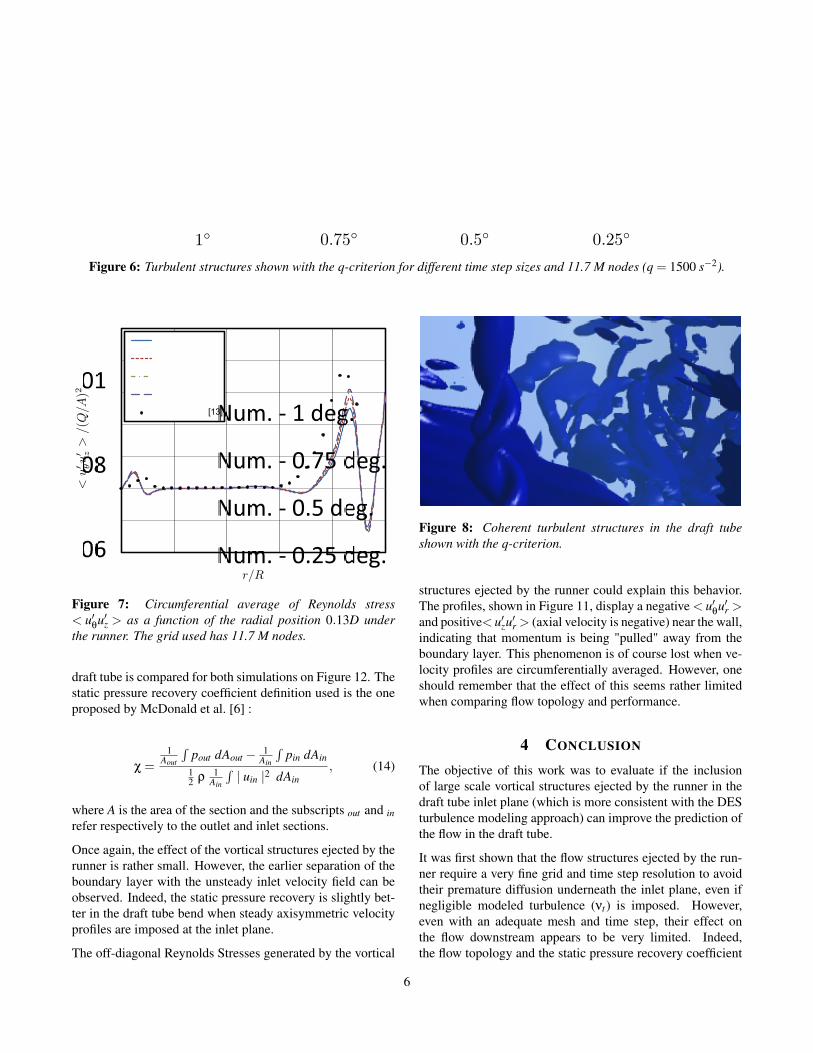
Figure 6: Turbulent structures shown with the q-criterion for different time step sizes and 11.7 M nodes (q = 1500 s−2).

[13]

Figure 7: Circumferential average of Reynolds stress< u′

θu′z > as a function of the radial position 0.13D under

the runner. The grid used has 11.7 M nodes.

draft tube is compared for both simulations on Figure 12. Thestatic pressure recovery coefficient definition used is the oneproposed by McDonald et al. [6] :

χ =

1Aout

∫pout dAout − 1

Ain

∫pin dAin

12 ρ

1Ain

∫| uin |2 dAin

, (14)

where A is the area of the section and the subscripts out and inrefer respectively to the outlet and inlet sections.

Once again, the effect of the vortical structures ejected by therunner is rather small. However, the earlier separation of theboundary layer with the unsteady inlet velocity field can beobserved. Indeed, the static pressure recovery is slightly bet-ter in the draft tube bend when steady axisymmetric velocityprofiles are imposed at the inlet plane.

The off-diagonal Reynolds Stresses generated by the vortical

Figure 8: Coherent turbulent structures in the draft tubeshown with the q-criterion.

structures ejected by the runner could explain this behavior.The profiles, shown in Figure 11, display a negative < u′

θu′r >

and positive< u′zu′r > (axial velocity is negative) near the wall,

indicating that momentum is being "pulled" away from theboundary layer. This phenomenon is of course lost when ve-locity profiles are circumferentially averaged. However, oneshould remember that the effect of this seems rather limitedwhen comparing flow topology and performance.

4 CONCLUSION

The objective of this work was to evaluate if the inclusionof large scale vortical structures ejected by the runner in thedraft tube inlet plane (which is more consistent with the DESturbulence modeling approach) can improve the prediction ofthe flow in the draft tube.

It was first shown that the flow structures ejected by the run-ner require a very fine grid and time step resolution to avoidtheir premature diffusion underneath the inlet plane, even ifnegligible modeled turbulence (νt ) is imposed. However,even with an adequate mesh and time step, their effect onthe flow downstream appears to be very limited. Indeed,the flow topology and the static pressure recovery coefficient

6

Saddle Point Saddle Point

Figure 9: Skin friction lines on the draft tube solid boundaries a) with the vortical flow structures injected at the inlet planeand b) with steady axisymmetric velocity profiles.

Figure 10: Time-averaged normal velocity field in the draft tube outlet bays a) with the vortical flow structures injected at theinlet plane and b) with steady axisymmetric velocity profiles.

7

Figure 11: Circumferentially averaged off-diagonal Reynolds Stress tensor components 0.13D under the runner with andwithout the vortical structures injected at the inlet plane (2D inlet vs Axisymmetric).

2D InletAxisymmetric

A

B

A B

Figure 12: Evolution in the draft tube of the static pressurerecovery coefficient χ with and without the vortical flow struc-tures injected at the inlet plane (2D inlet vs Axisymmetric).

were very similar to those obtained with a simulation wheresteady axisymmetric velocity profiles were specified at theinlet plane.

However, this investigation was performed at an operatingpoint close to the best efficiency point. Even though thevortical flow structures do not directly transfer a significantamount of momentum to the boundary layers, they could havea more significant interaction with the central vortical struc-ture at partial discharge, where it is stronger. Therefore, infuture works, a similar investigation could be performed atdifferent operating points, in order to generalize the presentconclusion.

ACKNOWLEDGEMENTS

The authors would like to thank Alstom Power & TransportCanada inc, the FQRNT and the NSERC for their financialsupport throughout this research project. Computations wereperformed on the Colosse supercomputer at Université Laval,under the auspices of Calcul Québec and Compute Canada.Finally, the authors would like to gratefully thank Sylvain Tri-don, of ALSTOM Hydro France, for sharing his experimentaldata.

REFERENCES

[1] P. B.-Vincent. Simulations avancées de l’écoulementturbulent dans les aspirateurs de turbines hydrauliques.Master’s thesis, Université Laval, 2010.

[2] M. J. Cervantes, U. Andersson, and H. M. Lövgren.Turbine-99 unsteady simulations - Validation. In Pro-ceedings of the 25th IAHR Symposium on HydraulicMachinery and Systems, Timisoara, September 2010.IAHR.

[3] J.-M. Gagnon, V. Aeschlimann, S. Houde, F. Flemming,S. Coulson, and C. Deschenes. Experimental investiga-tion of draft tube inlet velocity field of a propeller tur-bine. ASME Journal of Fluids Engineering, 134:10102–12, October 2012.

[4] ANSYS Inc. ANSYS CFX-Solver theory guide,November 2010.

[5] S. Mauri. Numerical Simulation and Flow Analysis ofan Elbow Diffuser. PhD thesis, École PolytechniqueFédérale de Lausanne, 2002.

[6] A. T. McDonald, R. W. Fox, and R. V. Van Dewoes-tine. Effects of swirling inlet flow on pressure recovery

8

in conical diffusers. AIAA Journal, 9(10):2014–2018,October 1971.

[7] F. R. Menter. Improved two-equation k−ω turbulencemodels for aerodynamic flows. Technical Memorandum103975, NASA, October 1992.

[8] F. R. Menter and M. Kuntz. Adaptation of eddy-viscosity turbulence models to unsteady seperated flowbehind vehicles. In Rose McCallen, Fred Browand,and James Ross, editors, The Aerodynamics of HeavyVehicles : Trucks, Buses, and Trains, pages 339–352.Springer, 2004.

[9] F. R. Menter, M. Kuntz, and R. Langtry. Ten years ofindustrial experience with the SST turbulence model. InK. Hanjalic, Y. Nagano, and M. Tummers, editors, Tur-bulence, Heat and Mass Transfer 4. Begell House, Inc.,2003.

[10] P. E. Smirnov and F. R. Menter. Sensitization of theSST turbulence model to rotation and curvature by ap-plying the Spalart-Shur correction term. In Proceedingsof ASME Turbo Expo 2008: Power for Land, Sea andAir, Berlin, Germany, June 2008. ASME.

[11] P. R. Spalart. Detached-eddy simulation. Ann. Rev.Fluid Mech., 41:181–202, 2009.

[12] P. R. Spalart, S. Deck, M. L. Shur, K. D. Squires, M. Kh.Strelets, and A. Travin. A new version of detached-eddysimulation, resistant to ambiguous grid densities. Theor.Comput. Fluid Dyn., 20:181–195, 2006.

[13] S. Tridon. Étude expérimentale des instabilités tour-billonnaires dans les diffuseurs de turbomachines hy-drauliques. PhD thesis, Institut Polytechnique deGrenoble, June 2010.

[14] S. Tridon, S. Barre, G. Dan Ciocan, and L. Tomas. Ex-perimental analysis of the swirling flow in a Francis tur-bine draft tube: Focus on radial velocity component de-termination. European Journal of Mechanics - B/Fluids,29(4):321 – 335, 2010.

9