Center for Turbulence ResearchProceedings of the Summer Program 2008

1

Coupling heat transfer solvers and large eddysimulations for combustion applications

By F. Duchaine†, S. Mendez†, F. Nicoud‡, A. Corpron¶, V. Moureau¶AND T. Poinsot†‖

A fully parallel environment for conjugate heat transfer has been developed and applied to twoconfigurations of interest for the design of combustion devices. The numerical tool is based ona reactive LES (Large Eddy Simulations) code and a solid conduction solver that can exchangedata via a supervisor. Two coupled problems, typical of gas turbine applications, are studied: (1)a flame/wall interaction problem is used to assess the precision of the coupled solutions dependingon the coupling frequency. For such an unsteady case, it is shown that the temperature and theflux across the wall are well-reproduced when the codes are coupled on a time scale which is of theorder of the smallest time scale. (2) An experimental film-cooled turbine vane is studied in order toreach a steady state. The solutions from the conjugate analyses and an adiabatic wall convectionare compared to experimental results. Pressure profiles on pressure and suction sides obtained byadiabatic and coupled simulations show a good agreement with experimental results. Comparedto the adiabatic simulation, it is found that the conjugate heat transfer case has a lower meanpressure side temperature due to the thermal conduction from this part to the plenum as well asfrom the pressure to the suction side of the blade. Thermal results show a very large sensitivity tomultiple parameters as the coupling strategy and LES models.

1. Introduction

Conjugate heat transfer is a key issue in combustion (Lefebvre 1999; Bunker 2007): the interactionof hot gases and reacting flows with colder walls is a key phenomenon in all chambers and is actuallya main design constraint in gas turbines. For example, multi-perforated plates are commonly usedin gas turbine combustion chambers to cool walls and they must be able to sustain the high fluxesproduced in the chamber. After combustion, the interaction of the hot burnt gases with the highpressure stator and the first turbine blades conditions the temperature and pressure levels reachedin the combustor, and therefore the engine efficiency.

Conjugate heat transfer is a difficult to accomplish and most existing tools are developed forchained (rather than coupled), steady (rather than transient) phenomena: the fluid flow is broughtto convergence using a RANS (Reynolds Averaged Navier-Stokes) solver for a given set of skintemperatures (Schiele & Wittig 2000; Garg 2002; Mercier et al. 2006). The heat fluxes predictedby the RANS solver are then transferred to a heat transfer solver which produces a new set ofskin temperatures. A few iterations are generally sufficient to reach convergence. There are cir-cumstances, however, where this chaining method must be replaced by a full coupling approach.Flames interacting with walls for example, may require a simultaneous resolution of the temper-ature within the solid and around it. More generally, the introduction of LES to replace RANSleads to full coupling since LES provides the unsteady evolution of all flow variables.

Fully coupled conjugate heat transfer requires that multiple questions be taken into account.Among them, two issues were considered for the present work:• The time scales of the flow and of the solid are generally very different. In a gas turbine, a

blade submitted to the flow exiting from a combustion chamber has a thermal characteristic timescale of the order of a few seconds, while the flow-through time along the blade is less than 1 ms.

† CERFACS, CFD Team, 42 Av Coriolis, 31057 Toulouse, France‡ Un. Montpellier II, France¶ TURBOMECA, Bordes, France‖ IMF Toulouse, INP de Toulouse and CNRS, 31400 Toulouse, France

2 F. Duchaine et al.

As a consequence, the frequency of the exchanges between the codes is critical for the precision,stability and restitution time of the computations.• Coupling the two phenomena must be performed on massively parallel machines where the

codes must be not only coupled but synchronized to exploit the power of the machines.

During this work, these two issues have been studied using two examples of conjugate heattransfer: (I) a flame interacting with a wall and (II) a blade submitted to a flow of hot gases. Bothproblems have considerable impact on the design of combustion devices.

2. Solvers and coupling strategies

The AVBP code is used for the fluid (Schonfeld & Rudgyard 1999; Roux et al. 2008). It solves thecompressible reacting Navier-Stokes equations with a third-order scheme for spatial differencingand a Runge-Kutta time advancement (Colin & Rudgyard 2000; Moureau et al. 2005). Boundaryconditions are handled with the NSCBC formulation (Poinsot & Veynante 2005; Moureau et al.2005).

For the resolution of the heat transfer equation within solids, a simplified version of AVBP, calledAVTP, was developed. It uses the same data structure as AVBP. It is coupled to AVBP using asoftware called PALM (Buis et al. 2005). For all present examples, the skin meshes are the samefor the fluid and the solid so that no interpolation error is introduced at this level.

The coupling strategy between AVBP and AVTP depends on the objectives of the simulationand is characterized by two issues:

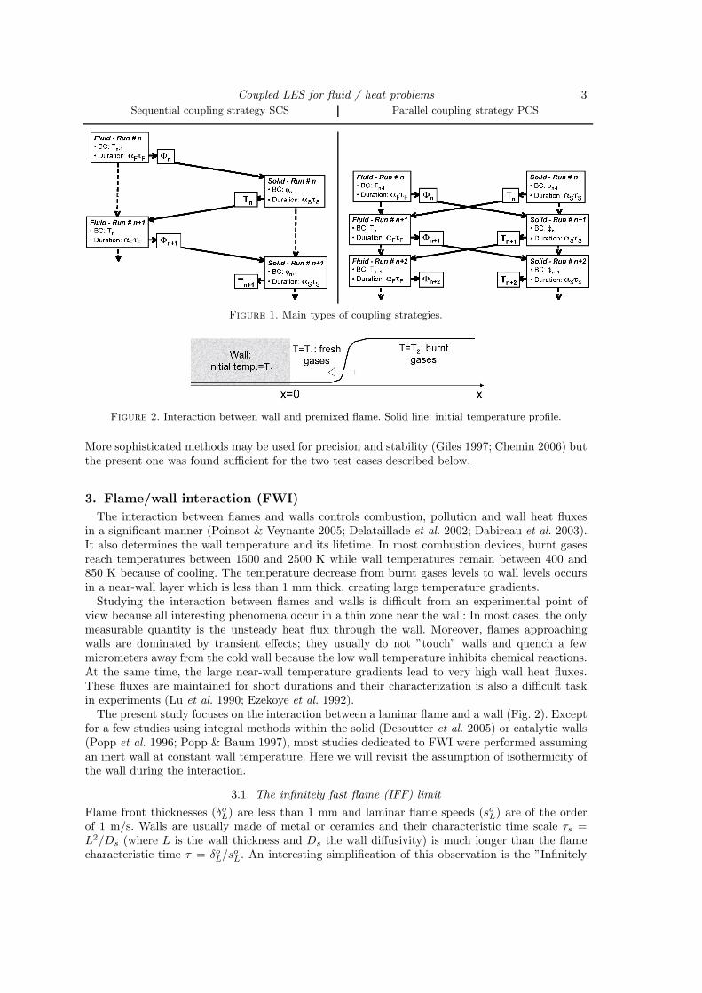
• Synchronization in physical time: The physical time computed by the two codes betweentwo information exchanges may be the same or not.† We will impose that between two couplingevents, the flow is advanced in time of a quantity αfτf where τf is a flow characteristic time.Simultaneously, the solid is advanced of a time αsτs where τs is a characteristic time for heatpropagation through the solid. Two limit cases are of interest: (1) αs = αf ensures that both solidand fluid converge to steady state at the same rate (the two domains are then not synchronized inphysical time) and (2) αfτf = αsτs ensures that the two solvers are synchronized in physical time.• Synchronization in CPU time: on a parallel machine, codes for the fluid and for the structure

may be run together or sequentially. An interesting question controlled by the execution modeis the information exchange. Figure 1 shows how heat fluxes and temperature are exchanged ina mode called SCS (Sequential Coupling Strategy) where the fluid solver after run n (physicalduration αfτf ) provides fluxes to the solid solver which then starts and gives temperatures Tn

(physical duration αsτs). In SCS mode, the codes are loaded into the parallel machine sequentiallyand each solver uses all available processors (N). Another solution is Parallel Coupling Strategy(PCS) where both solvers run together using information obtained from the other solver at theprevious coupling iteration (Fig. 1). In this case, the two solvers must share the P = Ps + Pf

processors. The Ps and Pf processors dedicated to the solid and the fluid, respectively, must besuch that:

Pf

P=

1

1 + Ts/Tf

(2.1)

where Ts and Tf are the execution times of the solid and fluid solvers, respectively (on one pro-cessor). Ts and Tf depend on αsτs and αfτf . Perfect scaling for both solvers is assumed here.

Note that both SCS and PCS questions are linked to the way information (heat fluxes and walltemperatures) are exchanged and to the implementation on parallel machines but are indepen-dent of the synchronization in physical time: PCS or SCS can be used for steady or unsteadycomputations. This paper focuses on the PCS strategy.

Finally,this work explores the simplest coupling method where the fluid solver provides heatfluxes to the solid solver while the solid solver sends skin temperatures back to the fluid code.

† For example, when a steady state solution is sought (i.e., to be used as initial condition for an unsteadycomputation), physical times for both solvers can differ.

Coupled LES for fluid / heat problems 3

Sequential coupling strategy SCS Parallel coupling strategy PCS

Figure 1. Main types of coupling strategies.

Figure 2. Interaction between wall and premixed flame. Solid line: initial temperature profile.

More sophisticated methods may be used for precision and stability (Giles 1997; Chemin 2006) butthe present one was found sufficient for the two test cases described below.

3. Flame/wall interaction (FWI)

The interaction between flames and walls controls combustion, pollution and wall heat fluxesin a significant manner (Poinsot & Veynante 2005; Delataillade et al. 2002; Dabireau et al. 2003).It also determines the wall temperature and its lifetime. In most combustion devices, burnt gasesreach temperatures between 1500 and 2500 K while wall temperatures remain between 400 and850 K because of cooling. The temperature decrease from burnt gases levels to wall levels occursin a near-wall layer which is less than 1 mm thick, creating large temperature gradients.

Studying the interaction between flames and walls is difficult from an experimental point ofview because all interesting phenomena occur in a thin zone near the wall: In most cases, the onlymeasurable quantity is the unsteady heat flux through the wall. Moreover, flames approachingwalls are dominated by transient effects; they usually do not ”touch” walls and quench a fewmicrometers away from the cold wall because the low wall temperature inhibits chemical reactions.At the same time, the large near-wall temperature gradients lead to very high wall heat fluxes.These fluxes are maintained for short durations and their characterization is also a difficult taskin experiments (Lu et al. 1990; Ezekoye et al. 1992).

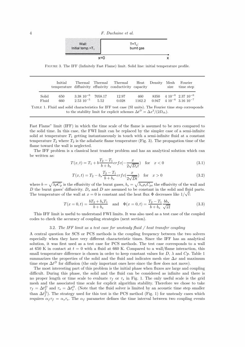
The present study focuses on the interaction between a laminar flame and a wall (Fig. 2). Exceptfor a few studies using integral methods within the solid (Desoutter et al. 2005) or catalytic walls(Popp et al. 1996; Popp & Baum 1997), most studies dedicated to FWI were performed assumingan inert wall at constant wall temperature. Here we will revisit the assumption of isothermicity ofthe wall during the interaction.

3.1. The infinitely fast flame (IFF) limit

Flame front thicknesses (δoL) are less than 1 mm and laminar flame speeds (so

L) are of the orderof 1 m/s. Walls are usually made of metal or ceramics and their characteristic time scale τs =L2/Ds (where L is the wall thickness and Ds the wall diffusivity) is much longer than the flamecharacteristic time τ = δo

L/soL. An interesting simplification of this observation is the ”Infinitely

4 F. Duchaine et al.

Figure 3. The IFF (Infinitely Fast Flame) limit. Solid line: initial temperature profile.

Initial Thermal Thermal Thermal Heat Density Mesh Fouriertemperature diffusivity effusivity conductivity capacity size time step

Solid 650 3.38 10−6 7058.17 12.97 460 8350 4 10−6 2.37 10−6

Fluid 660 2.53 10−5 5.52 0.028 1162.2 0.947 4 10−6 3.16 10−7

Table 1. Fluid and solid characteristics for IFF test case (SI units). The Fourier time step correspondsto the stability limit for explicit schemes ∆tD = ∆x2/(2Dth).

Fast Flame” limit (IFF) in which the time scale of the flame is assumed to be zero compared tothe solid time. In this case, the FWI limit can be replaced by the simpler case of a semi-infinitesolid at temperature T1 getting instantaneously in touch with a semi-infinite fluid at a constanttemperature T2 where T2 is the adiabatic flame temperature (Fig. 3). The propagation time of theflame toward the wall is neglected.

The IFF problem is a classical heat transfer problem and has an analytical solution which canbe written as:

T (x, t) = T1 + bT2 − T1

b + bs

erfc(− x

2√

Dst) for x < 0 (3.1)

T (x, t) = T2 − bs

T2 − T1

b + bs

erfc(x

2√

Dt) for x > 0 (3.2)

where b =√

λρCp is the effusivity of the burnt gases, bs =√

λsρsCps the effusivity of the wall andD the burnt gases’ diffusivity. Ds and D are assumed to be constant in the solid and fluid parts.The temperature of the wall at x = 0 is constant and the heat flux Φ decreases like 1/

√t:

T (x = 0, t) =bT2 + bsT1

b + bs

and Φ(x = 0, t) =T2 − T1

b + bs

bbs√πt

(3.3)

This IFF limit is useful to understand FWI limits. It was also used as a test case of the coupledcodes to check the accuracy of coupling strategies (next section).

3.2. The IFF limit as a test case for unsteady fluid / heat transfer coupling

A central question for SCS or PCS methods is the coupling frequency between the two solversespecially when they have very different characteristic times. Since the IFF has an analyticalsolution, it was first used as a test case for PCS methods. The test case corresponds to a wallat 650 K in contact at t = 0 with a fluid at 660 K. Compared to a wall/flame interaction, thissmall temperature difference is chosen in order to keep constant values for D, λ and Cp. Table 1summarizes the properties of the solid and the fluid and indicates mesh size ∆x and maximumtime steps ∆tD for diffusion (the only important ones here since the flow does not move).

The most interesting part of this problem is the initial phase when fluxes are large and couplingdifficult. During this phase, the solid and the fluid can be considered as infinite and there isno proper length or time scale to evaluate τf or τs in Fig. 1. The only useful scale is the gridmesh and the associated time scale for explicit algorithm stability. Therefore we chose to takeτf = ∆tDf and τs = ∆tDs . (Note that the fluid solver is limited by an acoustic time step smaller

than ∆tDf ). The strategy used for this test is the PCS method (Fig. 1) for unsteady cases whichrequires αfτf = αsτs. The αf parameter defines the time interval between two coupling events

Coupled LES for fluid / heat problems 5

0 100 200 300 400

-1e-05

-5e-06

0e+00

5e-06

Reduced time t+ = t/τf

Rel

ative

erro

ron

tem

per

atu

re

0 100 200 300 400-1

-0.5

0

0.5

1

1.5

Reduced time t+ = t/τf

Rel

ative

erro

ron

flux

Figure 4. Tests of the PCS method for the IFF case of Fig. 3. Effects of the coupling period between twoevents (measured by αs). Left: relative error on wall temperature at x = 0, right: relative error on wallflux at x = 0. Solid line: αf = 0.131, dashed: αf = 13.1, dots: αf = 65.5.

Initial Thermal Thermal Thermal Heat Density Mesh Timetemperature diffusivity effusivity conductivity capacity size scale

Solid 650 3.38 10−6 7058.17 12.97 460 8350 2 10−6 0.3Fresh gases 650 4.14 10−5 7.35 0.047 1168.9 0.977 4 10−6 30.45 10−6

Hot gases 2300 3.72 10−4 7.28 0.140 1441.6 0.262 4 10−6 30.45 10−6

Table 2. Fluid and solid characteristics for flame/wall interaction test case (SI units). The characteristictime τs for the solid is based on its thickness and heat diffusivity. The characteristic time scale for the fluidτf is based on the flame speed and thickness.

normalized by the fluid characteristic time. Values of αf ranging from 0.131 to 65.5 were testedfor this problem and Fig. 4 shows how the errors on maximum wall temperature and the wallheat flux change when αf changes. The IFF solution of Eq. (3.3) is used as the reference solution.Using values of αf larger than unity leads to relative errors which can be significant and to strongoscillations on the temperature and flux. As expected a full coupling of fluid and solid for thisproblem requires that values of αf of order unity be used which means to couple the codes on atime scale that is of the order of the smallest time scale (here the flow time scale).

3.3. Flame/wall interaction results

This section presents results obtained for a fully coupled FWI and compares them to the IFFlimit. The parameters used for the simulation (Table 2) correspond to a methane/air flame at anequivalence ratio of 0.8, propagating in fresh gases at a temperature T1 of 650 K at a laminarspeed so

L = 1.128 m/s. The adiabatic flame temperature is T2 = 2300 K. The wall is also initiallyat T1 = 650 K. The maximum time step corresponds to the Fourier stability criterion for the solidand to the CFL stability criterion for the fluid. These time steps are respectively ∆tFs = 0.59 µsand ∆tCFL

f = 0.0023 µs. For this fully coupled problem, the only free parameter is αf . The periodbetween two coupling events (αf τf = αsτs) determines the number of iterations performed by thegas solver during this time: Nit = αfτf/∆tCFL

f . As the cost of computing heat transfer in the solidfor this problem is actually negligible, no attempt was made to optimize the computation. Theeffect of mesh resolution in the gases was also checked and found to be negligible; for most runs,500 mesh points are used in the gases with a mesh size of 4 10−6 mm.

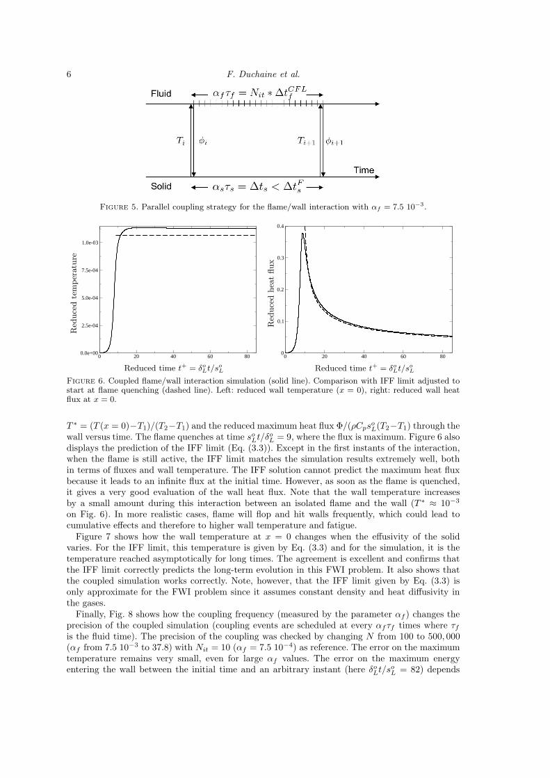
The coupling parameters for the presented case correspond to a PCS simulation with αf =7.5 10−3 leading to Nit = 100 in the gases accompanied by one iteration in the solid whereαs = 7.6 10−7 (Fig. 5). Figure 6 displays the wall-scaled temperature at the fluid and solid interface

6 F. Duchaine et al.

Figure 5. Parallel coupling strategy for the flame/wall interaction with αf = 7.5 10−3.

0 20 40 60 800.0e+00

2.5e-04

5.0e-04

7.5e-04

1.0e-03

Reduced time t+ = δoLt/so

L

Red

uce

dte

mper

atu

re

0 20 40 60 800

0.1

0.2

0.3

0.4

Reduced time t+ = δoLt/so

L

Red

uce

dhea

tflux

Figure 6. Coupled flame/wall interaction simulation (solid line). Comparison with IFF limit adjusted tostart at flame quenching (dashed line). Left: reduced wall temperature (x = 0), right: reduced wall heatflux at x = 0.

T ∗ = (T (x = 0)−T1)/(T2−T1) and the reduced maximum heat flux Φ/(ρCpsoL(T2−T1) through the

wall versus time. The flame quenches at time soLt/δo

L = 9, where the flux is maximum. Figure 6 alsodisplays the prediction of the IFF limit (Eq. (3.3)). Except in the first instants of the interaction,when the flame is still active, the IFF limit matches the simulation results extremely well, bothin terms of fluxes and wall temperature. The IFF solution cannot predict the maximum heat fluxbecause it leads to an infinite flux at the initial time. However, as soon as the flame is quenched,it gives a very good evaluation of the wall heat flux. Note that the wall temperature increasesby a small amount during this interaction between an isolated flame and the wall (T ∗ ≈ 10−3

on Fig. 6). In more realistic cases, flame will flop and hit walls frequently, which could lead tocumulative effects and therefore to higher wall temperature and fatigue.

Figure 7 shows how the wall temperature at x = 0 changes when the effusivity of the solidvaries. For the IFF limit, this temperature is given by Eq. (3.3) and for the simulation, it is thetemperature reached asymptotically for long times. The agreement is excellent and confirms thatthe IFF limit correctly predicts the long-term evolution in this FWI problem. It also shows thatthe coupled simulation works correctly. Note, however, that the IFF limit given by Eq. (3.3) isonly approximate for the FWI problem since it assumes constant density and heat diffusivity inthe gases.

Finally, Fig. 8 shows how the coupling frequency (measured by the parameter αf ) changes theprecision of the coupled simulation (coupling events are scheduled at every αfτf times where τf

is the fluid time). The precision of the coupling was checked by changing N from 100 to 500, 000(αf from 7.5 10−3 to 37.8) with Nit = 10 (αf = 7.5 10−4) as reference. The error on the maximumtemperature remains very small, even for large αf values. The error on the maximum energyentering the wall between the initial time and an arbitrary instant (here δo

Lt/soL = 82) depends

Coupled LES for fluid / heat problems 7

100 1000 10000 1e+05 1e+060

0.005

0.01

0.015

0.02

0.025

0.03

Wall effusivity

Red

uce

dte

mper

atu

re

Figure 7. Coupled flame/wall interaction simulation. Reduced wall temperature(T (x = 0) − T1)/(T2 − T1) vs. wall effusivity bs. Solid line: IFF limit, circles: coupled simulation.

0.01 0.1 1 10

1e-06

1e-05

0.0001

0.001

First O

rder

αf

Rel

ative

erro

ron

wall

tem

per

atu

re

0.01 0.1 1 10

0.01

0.1

1

First

Ord

er

αf

Rel

ative

erro

ron

ener

gy

Figure 8. Flame/wall interaction simulation. Left: relative error on wall temperature (x = 0) fromt+ = δo

Lt/soL = 0 to t+ = 82, right: relative error on the energy fluxed into the wall during the same

period.

strongly on αf . As expected from results obtained for the IFF problem only (previous section),coupling the two solvers less often that τf (αf > 1) leads to errors larger than 10% on the energyfluxed into the wall. The errors on temperature and energy fluxed into the wall converge both to0 when αf decreases with an order close to 1.

4. Blade cooling

The second example studied during this work is the interaction between a high-speed flow anda cooled blade. This example is typical of one of the main problems encountered during the designof combustion chambers (Bunker 2007; Bogard & Thole 2006): The hot flow leaving the combustormust not burn the turbine blades or the vanes of the high-pressure stator. Predicting the vanes’temperature field (which are cooled from the inside by cold air) is a major research area (Holmeret al. 2000; Medic & Durbin 2002; Garg 2002). Here an experimental setup (T120D blade) developedwithin the AITEB-1 European project was used to evaluate the precision of the coupled simulations(Fig. 9). The temperature difference between the mainstream (T2 = 333.15 K) and cooling (T1 =303.15 K) airs is limited to 30 K to facilitate measurements. Experimental results include pressuredata on the blade suction and pressure sides as well as temperature measurement on the pressureside.

The computational domains for both the fluid and the structure contain only one spanwise pitchof the film cooling hole pattern (z-axis on Fig. 9), with periodicity enforced at each end. Thissimplification assumes no end-wall effects, but retains the three-dimensionality of the flow andgreatly reduces the number of tetrahedral cells required to model the blade: about 6.5 million

8 F. Duchaine et al.

Figure 9. Configuration for blade cooling simulation: the T120D blade (AITEB-2 project).

Inlet static Inlet total Inlet total Flow Thermal Heat Time Timetemperature temperature pressure rate conductivity capacity scale step ∆tm

f

Mainstream T2 = 333.15 T t2 = 339.15 P t

2 = 27773 0.0185 2.6 10−2 1015 0.001 9.80 10−8

Cooling air T1 = 303.15 T t1 = 303.15 P t

1 = 29143 0.000148 2.44 10−2 1015 0.0006 9.80 10−8

Table 3. Flow characteristics for the blade cooling case (SI units). The fluid time scales are based on theflow-through times in and around the blade. The characteristic fluid time scale τf is the maximum of thistime, i.e., τf = 0.001. The time step ∆tm

f is limited by the acoustic CFL number (0.7).

cells to discretize the fluid and 600, 000 for the solid. A periodicity condition is also assumed inthe y-direction. The WALE subgrid model (Nicoud & Poinsot 1999) is used in conjunction withnon-slipping wall conditions. As shown in Fig. 9, the three film-cooling holes and the plenum areincluded in the domain: jet 2 is aligned with the main flow (in the xy-plane) while jets 1 and 3have a compound orientation. The mean blowing ratio (ratio of a jet momentum on the hot flowmomentum) of the jets based on a hot gases velocity of 35 ms−1 is approximately 0.4.

Tables 3 and 4 summarize the properties of the gases and of the solid used for the simulation.At each coupling event, fluxes and temperature on the blade skin are exchanged as described inFig. 1. During this work, only a steady state solution within the solid was sought so that timeconsistency was not ensured during the coupling computation. The converged state is obtainedwith a two-step methodology:

(a) Initialization of the coupled calculation that includes:• a thermal converged adiabatic fluid simulation,• a thermal converged isothermal solid computation with boundary temperatures given by thefluid solution,

(b) Coupled simulation.

Convergence is investigated by plotting the history of the total flux on the blade (which mustgo to zero) and of the mean, minimum and maximum blade temperatures. Figures 10 and 11 showthese results for two variants of the PCS strategy. In the first one, fluxes and temperature areexchanged at each coupling step while for the second one, relaxation is used and temperature andfluxes imposed at each coupling iteration n are written as fn = afn−1 + (1 − a)fn∗ where fn∗ is

Coupled LES for fluid / heat problems 9

Thermal Heat Density Thermal Time Timeconductivity capacity diffusivity scale τs step

0.184 1450 1190 1.07 10−7 34.22 1.71 10−3

Table 4. Solid characteristics for the blade-cooling case (SI units). The time scale τs is computed usingthe thermal diffusivity and the blade minimum thickness.

0 1 2 3 4 5 6 7 8200

225

250

275

300

325

350

375

400

Reduced time t+ = t/τs

Tem

per

atu

re

0 1 2 3 4 5 6 7 8

0

1

2

3

Reduced time t+ = t/τs

Tota

lw

all

flux

Figure 10. Time evolution of minimum and maximum temperatures in the blade (left) and total heatflux through the blade with (solid) and without (dashed) relaxation.

the value obtained by the other solver at iteration n and a is a relaxation factor (typically a = 0.6).Without relaxation, the system becomes unstable and convergence almost impossible.

At the converged state, the total flux reaches zero: the flux entering the blade is evacuated intothe cooling air in the plenum and in the holes (Fig. 11). Note however that the analysis of fluxeson the blade skin shows that, even though the blade is heated by the flow on the pressure side, itis actually cooled on part of the suction side because the flow accelerates and cools down on thisside. Due to the acceleration in the jets, heat transfer in the holes and plenum are of the sameorder. Compared to the external flux, plenum and hole fluxes converge almost linearly. Oscillationsin the external flux evolution are linked with the complex flow structure developing around theblade.

At the converged state, results can be compared to the experiment in terms of pressure profileson the blade (on both sides) and of temperature profiles on the pressure side. Pressure fields aredisplayed in terms of isentropic Mach numbers Mis computed by

Mis =

√

√

√

√

2

γ − 1

[

(

P t2

P tw

)

γ−1

γ

− 1

]

(4.1)

where P t2 and P t

w are the total pressure of the mainstream and at the wall. Figure 12 displays anaverage field of isentropic Mach number obtained by LES and by the experiment. The comparisonof the adiabatic simulation and the coupled one shows that these profiles are only weakly sensitiveto the thermal condition imposed on the blade. Although the shock position on the suction side isnot perfectly captured, the overall agreement between LES and experimental results is fair.

Temperature results are displayed in terms of reduced temperature Θ = (T t2−T )/(T t

2−T t

1) where

T t2 and T t

1 are the total temperatures of the main and cooling streams (Table 4) and T is the localwall temperature. Θ measures the cooling efficiency of the blade. Figure 13 shows measurements,adiabatic and coupled LES results for Θ spanwise averaged along axis x. As expected, the coolingefficiency obtained with the adiabatic computation is lower than the experimental values: The

10 F. Duchaine et al.

0 5 10 15 20 25 30

-0.8

-0.6

-0.4

-0.2

0

0.2

0.4

0.6

0.8

Reduced time t+ = t/τs

Hea

tfluxes

Figure 11. Time evolution of heat fluxes through the blade: external flux (solid line), plenum (dashed),holes sides (dot), sum of all fluxes (dot dashed).

0 0.2 0.4 0.6 0.8 10

0.2

0.4

0.6

0.8

1

Reduced abscissa

Isen

tropic

Mach

num

ber

Mis

Figure 12. Isentropic Mach number along the blade. Solid line: coupled LES, circles: adiabatic LES,squares: experiment.

adiabatic temperature field over-predicts the real one. The main contribution of conduction in theblade is to reduce the wall temperature on the pressure side.

The reduced temperature distribution on the pressure side (Fig. 14) shows that the peak tem-perature occurs at the stagnation point (reduced abscissa close to 0). The temperature at thestagnation point is reduced compared to the adiabatic wall prediction, leading to local values ofθ of the order of 0.2. The thermal effects of the cooling jets on the vane are clearly evidenced byFig. 14. Jet 3 seems to be the most active in the cooling process by protecting the blade from thehot stream until a reduced absissa of 0.5 and then impacting the vane between 0.5 and 0.6.

The reduced temperature obtained during this work over-estimates experimental measurements.In particular, the strong acceleration caused by the blade induces large thermal gradients at thetrailing edge. This phenomenon, not-well resolved by the computations, leads to a non-physicalvalues of cooling efficiency. Nevertheless, these results have shown great sensitivity to multipleparameters, not only of the coupling strategy but also of the LES models for heat transfer andwall descriptions. Additional studies will be continued after the Summer Program.

Coupled LES for fluid / heat problems 11

0 0.2 0.4 0.6 0.8 10

0.2

0.4

0.6

Reduced abscissa

Cooling

effici

ency

Figure 13. Cooling efficiency Θ versus abscissa on the pressure side at steady state. Dashed line: adiabaticLES, solid line: coupled LES, symbols: experiment from UNIBW, vertical dashed lines: position of the holes.

Figure 14. Spatial distribution of reduced temperature θ on the pressure side of the blade. Thecomputational domain is duplicated one time in the z-direction.

5. Conclusions

Conjugate heat transfer calculations have been performed for two configurations of importancefor the design of gas turbines with a recently developed massively parallel tool based on a LESsolver. (1) An unsteady flame/wall interaction problem was used to assess the precision of coupledsolutions when varying the coupling period. It was shown that the maximum coupling period thatallows the temperature and the flux across the wall to reproduce well is of the order of the smallesttime scale of the problem. (2) Steady convective heat transfer computation of an experimental film-cooled turbine vane showed how thermal conduction in the blade tends to reduce wall temperaturecompared to an adiabatic case. Further studies on LES models, coupling strategy and experimentalconditions are needed to improve the quality of the results compared to the experimental coolingefficiency.

Acknowledgments

The help of L. Pons, from TURBOMECA, and of the AITEB-1 and AITEB-2 consortium re-garding access to the experimental results is gratefully acknowledged.

REFERENCES

Bogard, D. G. & Thole, K. A. 2006 Gas turbine film cooling. J. Prop. Power 22 (2), 249–270.

Buis, S., Piacentini, A. & Declat, D. 2005 PALM: A Computational Framework for assem-bling High Performance Computing Applications. Concurrency and Computation: Practiceand Experience .

Bunker, R. S. 2007 Gas turbine heat transfer: Ten remaining hot gas path challenges. Journalof Turbomachinery 129, 193–201.

12 F. Duchaine et al.

Chemin, S. 2006 Etude des interactions thermiques fluides-structure par un couplage de codes decalcul. PhD thesis, Universite de Reims Champagne-Ardenne.

Colin, O. & Rudgyard, M. 2000 Development of high-order Taylor-Galerkin schemes for un-steady calculations. J. Comput. Phys. 162 (2), 338–371.

Dabireau, F., Cuenot, B., Vermorel, O. & Poinsot, T. 2003 Interaction of H2/O2 flameswith inert walls. Combust. Flame 135 (1-2), 123–133.

Delataillade, A., Dabireau, F., Cuenot, B. & Poinsot, T. 2002 Flame/wall interactionand maximum heat wall fluxes in diffusion burners. Proc. Combust. Inst. 29, 775–780.

Desoutter, G., Cuenot, B., Habchi, C. & Poinsot, T. 2005 Interaction of a premixed flamewith a liquid fuel film on a wall. Proc. Combust. Inst. 30, 259–267.

Ezekoye, O. A., Greif, R. & Lee, D. 1992 Increased surface temperature effects on wall heattransfer during unsteady flame quenching. In 24th Symp. (Int.) on Combustion, pp. 1465–1472.The Combustion Institute, Pittsburgh, Penn.

Garg, V. 2002 Heat transfer research on gas turbine airfoils at NASA GRC. International Journalof Heat and Fluid Flow 23 (2), 109–136.

Giles, M. 1997 Stability analysis of numerical interface conditions in fluid-structure thermalanalysis. International Journal for Numerical Methods in Fluids 25 (4), 421–436.

Holmer, M.-L., Eriksson, L.-E. & Sunden, B. 2000 Heat transfer on a film cooled inlet guidevane. In Proceedings of the ASME Heat Transfer Division, American Society of MechanicalEngineers , vol. 366-3, pp. 43–50. Orlando, Florida.

Lefebvre, A. H. 1999 Gas Turbines Combustion. Taylor & Francis.

Lu, J. H., Ezekoye, O., Greif, R. & Sawyer, F. 1990 Unsteady heat transfer during sidewall quenching of a laminar flame. In 23rd Symp. (Int.) on Combustion, pp. 441–446. TheCombustion Institute, Pittsburgh, Penn.

Medic, G. & Durbin, P. A. 2002 Toward improved film cooling prediction. J. Turbomach. 124,193–199.

Mercier, E., Tesse, L. & Savary, N. 2006 3d full predictive thermal chain for gas turbine. In25th International Congress of the Aeronautical Sciences . Hamburg, Germany.

Moureau, V., Lartigue, G., Sommerer, Y., Angelberger, C., Colin, O. & Poinsot, T.

2005 High-order methods for DNS and LES of compressible multi-component reacting flowson fixed and moving grids. J. Comput. Phys. 202 (2), 710–736.

Nicoud, F. & Poinsot, T. 1999 DNS of a channel flow with variable properties. In Int. Symp.On Turbulence and Shear Flow Phenomena.. Santa Barbara, Calif.

Poinsot, T. & Veynante, D. 2005 Theoretical and numerical combustion. R.T. Edwards, 2ndedition.

Popp, P. & Baum, M. 1997 An analysis of wall heat fluxes, reaction mechanisms and unburnthydrocarbons during the head-on quenching of a laminar methane flame. Combust. Flame108 (3), 327–348.

Popp, P., Baum, M., Hilka, M. & Poinsot, T. 1996 A numerical study of laminar flamewall interaction with detailed chemistry: wall temperature effects. In Rapport du Centre deRecherche sur la Combustion Turbulente (ed. T. J. Poinsot, T. Baritaud & M. Baum), pp.81–123. Rueil Malmaison: Technip.

Roux, A., Gicquel, L. Y. M., Sommerer, Y. & Poinsot, T. J. 2008 Large eddy simulationof mean and oscillating flow in a side-dump ramjet combustor. Combust. Flame 152 (1-2),154–176.

Schiele, R. & Wittig, S. 2000 Gas turbine heat transfer: Past and future challenges. Journalof Propulsion and Power 16 (4), 583–589.

Schonfeld, T. & Rudgyard, M. 1999 Steady and unsteady flows simulations using the hybridflow solver AVBP. AIAA Journal 37 (11), 1378–1385.