Progress Towards Large-Eddy Simulations for Prediction of ...

Progress Towards Large-Eddy Simulations for

Prediction of Realistic Nozzle Systems

James R. DeBonis ∗

NASA Glenn Research Center, Cleveland, Ohio 44135

This paper reviews the current state of large-eddy simulation (LES) for nozzle flowsand discusses the issues which currently limit its application to simulating realistic noisereducing nozzle systems. LES has been used extensively to compute the flowfield of tur-bulent jets. It has shown the potential to significantly impact the design and analysis offuture noise suppressing nozzle systems through improved accuracy and physical insight.There are many issues that must be resolved before an accurate prediction can be madefor a complex nozzle system. Foremost, the high-order schemes used in LES must beadapted to be used in flexible gridding systems which can handle complex geometries.Hybrid Reynolds Averaged Navier-Stokes/LES schemes with appropriate interfaces mustbe developed to model the region near the nozzle exit and initial shear layer. Also, im-proved accuracy without reliance on empirical adjustments of simulation parameters mustbe demonstrated.

I. Introduction

Regulations on aircraft noise have become increasingly more stringent throughout the world. A largecontributor to aircraft noise at takeoff is the noise produced from the exhaust system, jet noise. As a result,jet noise reduction has become a critical technology for the aerospace industry. Significant noise reductionsfor turbofan engines have resulted from increasing the engine’s bypass ratio. However, additional noisereduction technology is needed for low bypass engines and to meet future regulations for the high bypassratio engines.

One such technology that is currently flying is the chevron nozzle (figure 1). The serrated edge of thechevron nozzle increases the mixing of the exhaust streams and modifies the turbulent characteristics in thejet, reducing noise [1]. This has been installed on several commercial aircraft engines already.

There are several other noise reduction concepts currently being studied. Most concepts, such as plasmaactuators [2], fluidic injection [3], tabs [4,5] and lobed mixers (figure 2) [6] aim to increase mixing and modifythe jet turbulence similar to the chevron nozzle. Papamoschou has developed a series of concepts that arereferred to as offset fan flow technology nozzles [7, 8]. The main idea is to divert the fan flow below theengine and change the noise directivity and intensity. Implementation of the offset fan flow idea would bethrough devices such as vanes or wedges (figure 3).

Design and analysis of these concepts can be greatly enhanced through the use of computational fluiddynamics (CFD). CFD has been successfully used for years the development of other aerospace components.To date almost all CFD for design and development has been steady Reynolds Averaged Navier-Stokes(RANS) calculations. However, RANS turbulence models have not proved accurate for jet flows [9]. Muchwork has been done in the area of advanced RANS models specifically for jets [10–12]. The results have beenmixed, and generalizing these models to wide range of flow conditions and geometries may not be possible.RANS is also limited in the information it can provide. For most jet applications a two equation k-ε or k-ωis used [13]. The models can only provide a simple statistical representation of the turbulence in the formof the turbulent kinetic energy and a local length scale.

Acoustic predictions based on RANS solutions are done using the acoustic analogy [14,15]. This acousticmodeling relies heavily on modeling the acoustic source based on the RANS solutions [16]. The results

∗Aerospace Engineer, Inlet & Nozzle Branch, 21000 Brookpark Rd., MS 86-7, Associate Fellow AIAA

1 of 14

American Institute of Aeronautics and Astronautics

44th AIAA Aerospace Sciences Meeting and Exhibit9 - 12 January 2006, Reno, Nevada

AIAA 2006-487

This material is declared a work of the U.S. Government and is not subject to copyright protection in the United States.

from this method are reasonable for cold round jets. Results are poor for heated jets and non-axisymmetricgeometries.

Large-Eddy Simulation (LES) is the next logical step towards improved jet predictions. Over the lastdecade LES has been increasingly used due to the growth in computing power. LES is an unsteady methodwhich directly computes the large-scale turbulent structures and reserves modeling for the small-scale tur-bulence. Since the large-scale turbulence carries most of the turbulent energy, very good predictions of theturbulent flowfield are possible. The direct simulation of large-scale structures can significantly enhance ourunderstanding of the flow and lead to better noise reduction strategies and improved designs.

The large-eddy simulation of the jet near field captures the nonlinear sound generation process. It ispossible but not efficient to carry the simulation to the acoustic farfield to compute the noise directly. Thepropagation of the sound to the farfield is a linear process and can instead be predicted by several simplermethods. Shih et al. gives a good discussion and evaluation of these methods [17].

LES has the potential to vastly improve the prediction of jet flows and impact designs of noise suppressingnozzles. However, there is much work that needs to be done before LES can be used reliably in this manner.The intent of this paper is to provide a goal for developers of LES methods, give an overview of the currentstatus of LES and identify issues that must be addressed to reach this goal.

II. Examples of LES of Jet Flows

Jet flows have been a popular application of LES. This section summarizes a representative sample ofthe work to date. Much of the work has focused on unheated round jets, the exceptions to this are noted.

Lele and coworkers performed several simulations of hot and cold Mach 0.9 jet at low to moderateReynolds number using a consistent approach [18–20]. They employ a sixth-order compact differencing inspace [21] and an explicit low-dispersion Runge-Kutta (LDRK) differencing in time. They use a dynamicsub-grid model. The solution is explicitly filtered. The inflow boundary condition consists of a velocityprofile with sinusoidal forcing of the axial velocity component and random forcing of the azimuthal velocitycomponent.

Bogey and Bailly have simulated several subsonic jets [22–24]. Their method uses an thirteen pointfinite-differencing in space. The finite difference stencil is optimized to minimize the dispersion error and isbased on Tam and Webb’s dispersion relation preserving (DRP) scheme [25]. They also use a LDRK schemefor time advancement. Their earlier work employed explicit modeling of the sub-grid scales. However, recentwork has relied on filtering without sub-grid models. They have also examined the influence of eddy viscosityon the effective Reynolds number of the flow.

Shur, Spalart and Strelets have taken a different approach [26,27]. They have adapted a RANS code whichuses a finite volume approach that employs the Roe scheme. The fluxes are computed with hybrid fifth-orderupwind/fourth-order central differences. Limiters are used in the presence of shocks. Time advancement isdone using an implicit second-order scheme. This simulation does not use a sub-grid scale model. They relyon the numerical dissipation of the scheme to remove energy that would be dissipated by the small scales.The authors have simulated a chevron nozzle by modifying the inflow boundary condition and altering thegrid at the inflow plane.

These simulations all utilized an inflow boundary condition that specifies the jet velocity profile. Thevelocity profiles are typically represented using a hyperbolic tangent function. With the exception of Shur,Spalart and Strelets, some type of unsteady perturbation is imposed. The development of the shear layer isdependent on the initial shear layer thickness as well as the type, frequency and magnitude of the imposedvelocity perturbations.

DeBonis has performed large-eddy simulations on a supersonic jet, Mach 1.4 and a subsonic jet, Mach0.9, where the nozzle geometry was modeled [28,29]. This avoids the ad hoc specification of inflow conditionsby directly solving the internal nozzle flow. However the accuracy of this approach is compromised by thedifficulty of resolving the small-scale structures in the nozzle boundary layer. It can be argued that thesmall-scale turbulence from the nozzle boundary layer does not play a significant role in the downstreamdevelopment of the jet, and that it is most important to correctly model the bulk properties of the initialshear layer.

Paliath and Morris [30] performed a simulation which combined both approaches. The nozzle was includedin the simulation to obtain the correct bulk properties of the boundary layer/initial shear layer. They alsoimposed small perturbations in the shear layer to simulate the small-scale turbulence that could not be

2 of 14


modeled. Their analyses included both round and rectangular nozzle geometries.

III. Approaches to LES of Jet Flows

There appears to be two general philosophical approaches to the application of LES to jet flows, therigorous and the practical. Both approaches have yielded reasonable results in their targeted application.

A. Rigorous LES

The approach which will be called Rigorous LES, involves careful attention to all aspects of the LES proce-dure. Each part of the LES solution is explicitly addressed: numerical error, filtering and sub-grid modeling.Careful attention is paid to minimizing numerical error. High-order schemes which minimize dispersion anddissipation errors are used. Explicit filtering of the solution is typically performed. The filtering processremoves the small unresolved scales from the solution in a mathematically consistent manner and has theadded benefit of enhancing numerical stability. The sub-grid scales are modeled using any one of a numberof sub-grid models. These calculations are typically performed for very low Reynolds number round jets.In addition these approaches have traditionally been used for simple geometries. A low Reynolds numberflow has a narrower range of turbulent scales and enables better resolution, decreasing the importance of thesub-grid model. The benefit of this approach is the ability to evaluate and control the contributions of eachsolution component. The drawback is the cost and complexity of the system.

B. Practical LES

Practical LES takes a more pragmatic approach, attempting to get a reasonable answer with less regardto every detail of the analysis (this is not a statement on the quality of the work). Instead of separatecomponents for filtering and sub-grid modeling one or both of these are usually combined with the numericalscheme. More dissipative schemes such as those found in most RANS codes are used. These analyses areusually performed for complex geometries and at high Reynolds number. More empiricism may be neededto achieve a good solution. Many simulations which fall into this category use codes that have been adoptedfrom RANS. In these cases, the codes have more flexible grid requirements and complex geometries are easierto model.

IV. Issues

A. Numerical Scheme

The numerical scheme used plays a major role in the simulation’s accuracy and can have a significant effect onhow the other components of the simulation work. A wide variety of numerical schemes have been employedfor the LES of jet flows. A large majority of LES has been performed using schemes that have a high-orderof accuracy.

1. Explicit Finite Difference Schemes

Explicit finite difference methods include both the traditional finite difference stencils and the optimizeddispersion relation preserving (DRP) type schemes. For a traditional finite difference stencil the coefficientsare chosen to maximize the order of accuracy of the scheme. Newer optimized stencils are based on Tam andWebb’s DRP scheme [25]. In this method, the order of accuracy does not determine the stencil coefficients.Instead, the coefficients are chosen to minimize the error of the scheme over a limited range of wave numbers.Optimized schemes are a good choice for large-eddy simulation. Since the range of scales that must be resolvedis finite, it makes sense to minimize the error over this range. Furthermore it must be pointed out that anumerical scheme’s order of accuracy only indicates how the error will be reduced with grid refinement anddoes not indicate the magnitude of the error for a given grid size. Tam and Webb’s original DRP schemeuses a seven point stencil. Bogey and Bailly’s scheme uses a thirteen point stencil [31]. Such a wide stencilmakes implementation of the scheme difficult near boundaries and block interfaces.

3 of 14


2. Compact Schemes

Compact schemes implicitly compute the derivative [21,32,33]. An example of a sixth-order compact schemewhich results in a tridiagonal system is shown [34].

115

(14δ2xfj + δ4xfj) =15

��df

dx

�j+1

+ 3�

df

dx

�j

+�

df

dx

�j−1

�(1)

This enables more accurate schemes for a given size stencil. In addition, these schemes have excellentresolution in wave number space. Their implicit nature increases the complexity and computational costof the scheme. But, the narrow stencil aids in implementation near boundaries and block interfaces. Somecodes utilizing compact schemes for jet analyses have been developed by Lele [21], Gaitonde and Visbal [35],and Hixon [32].

3. Artificial Dissipation/Filtering

The schemes discussed so far are central difference. This is done to eliminate the dissipative error terms andpreserve the turbulent structures. The lack of inherent dissipation in the scheme means that the solutionwill be unstable. Artificial dissipation, frequently in the form of a filter, is added to maintain stability.Compact filters have been developed by Lele [21], Gaitonde and Visbal [33] and Hixon [36]. Other filtersby have been developed by Kennedy and Carpenter [37], Vasilyev [38] and Bogey and Bailly [31]. Theseschemes do not capture shocks well and they have been applied primarily to subsonic jets. Some work hasbeen done to improve shock capturing by combining filters; a switch, typically based pressure gradient, isused to apply the more dissipative shock capturing filter near the shock and apply the less dissipative filterelsewhere [39,40].

4. Upwinded Schemes

The vast majority of modern CFD codes are finite volume RANS solvers utilizing upwinded schemes such asthe popular Roe scheme [41]. Upwinded schemes are dissipative and tend to damp turbulent structures thatLES hopes to capture. Such general purpose solvers may not be immediately appropriate for high qualityLES run in the same manner as RANS. However, by increasing the order of the schemes, and subsequentlyreducing the amount of dissipation, they have proven successful in some implementations [26,27]. They areparticularly suited for the Monotonically Integrated Large-Eddy Simulation (MILES) approach [42,43].

The importance of the spatial discretization scheme in LES cannot be overstated. As illustration, figure 4shows the difference between two numerical schemes with differing amounts of dissipation. The simulations,from Shur, Spalart and Strelets [26], are identical except for the fact that the first uses a third orderupwinded scheme and the second uses a fifth-order upwinded scheme. The latter scheme has significantlyless dissipation and therefore has better resolution of the turbulent structures.

5. Temporal Discretization

A lot of attention has been focused on the proper spatial discretization for LES. In contrast relatively littleeffort has been given to the temporal scheme. Some work has been done examining the error due to thetemporal discretization on numerical solutions in one-dimension [44]. There, it was clearly shown that theorder of the numerical scheme was determined by the lower-order discretization (temporal or spatial). Ahigh-order spatial discretization can be comprised by the error of a lower-order temporal scheme. This hasnot been extended to multiple dimensions where additional error in the spatial discretization complicatematters. Explicit Runge-Kutta schemes are used for most analyses; typically combined with compact orexplicit finite difference schemes. Both the standard four-stage fourth-order scheme [45] and optimized low-dissipation and low-dispersion schemes are used [46–48]. The optimized schemes add additional stages toreduce error. Regardless of the scheme it is prudent to perform a simple check of the effect of the temporaldiscretization error by repeating a portion of the calculation using a smaller time step.

B. Grid

Grid requirements will obviously vary based on the numerical scheme used. Issues such as the number ofgrid points required, grid skewness and the allowable rate of grid stretching are highly dependent on the

4 of 14


individual numerical method. Some but not all researchers have attempted to quantify these requirementsfor their particular schemes. Ideally isotropic grids would be used for these calculations. But, computinglimitations force the implementation of grid stretching to cluster points in the regions of interest.

Many analysis codes used for jet LES have limited geometric flexibility. Most written for jet analyseshave used a cylindrical coordinate system, a natural choice for a round jet. Others have used a cartesiansystem for simplicity in the numerical implementation [49, 50]. As the technology begins to move beyondstudies of simple round jets it will be necessary to add geometric flexibility by adopting generalized curvilinearcoordinates. This will enable a transition to studies of more realistic nozzle systems with complex geometries.

Generalized curvilinear coordinates may not be enough to tackle the most difficult nozzle systems. RANSanalyses of complex nozzle systems use flexible multi-block grids with varying topologies [51–54]. LESsimulations do utilize multiple grid blocks to enable parallel computation. But the grid blocks are subdividedfrom a single grid, which enables simple point matched interfaces through overlapping or ghost cells. Blockinterfaces that maintain high-order of accuracy must be developed. Non-point matched interfaces will bevery useful for geometry modeling and to coarsen the grid away from regions of interest.

Unstructured grids offer a solution to the difficulties faced in multiblock structured grids. Howeverdeveloping high-order schemes for unstructured grids is a difficult task. Some work has begun in thisarea [55–57]. However there is a lot of work to be done before this technology can be implemented.

Pope advocates the use of solution adaptive gridding to eliminate the subjective specification of theresolved turbulent length scale [58]. This idea is an excellent way to insure proper resolution. But it willplace a great dependence on increased grid flexibility in LES codes.

C. Boundary Conditions

1. Outflow Boundary

There have been two on-going issues regarding boundary conditions for jet LES. The first is a non-reflectingoutflow boundary condition. Waves that reflect from the outflow back into the computational domain cancontaminate the solution. There are many self-contained boundary conditions written to eliminate thesereflections using characteristic wave relations [59–62]. These methods have had moderate success but can bedifficult to implement in a general way. Many researchers have had success with the more ad hoc approachof creating what is referred to as absorbing layers/sponge regions/exit zones near the boundary [63]. Theseare areas of gradually increasing grid spacing. The increased grid spacing combined with dissipation of thenumerical scheme serves to damp waves as they near the boundary. Additional dissipation or source termsin the governing equations are sometimes added to increase the damping.

2. Specification of the Jet

The second boundary condition issue, the inflow boundary, is perhaps the most critical need for LES ofcomplex nozzle systems. The method used to specify the jet is critical to the downstream development offlow structures. A common approach to specifying the inflow is through a velocity profile. The profile isfrequently based on a hyperbolic tangent function and the initial mixing layer thickness is specified. Anunsteady component can be added to simulate the initial turbulence levels. This artificial “forcing” of theshear flow can greatly influence the mixing of the jet. Great care must be taken to avoid biasing the solutionand affecting the acoustic farfield. Glaze and Frankel found that random fluctuations based on a Gaussiandistribution dissipated quickly downstream [50]. Bogey and Bailly studied both the effects of forcing differentmodes and the effect of shear layer thickness, with significant differences in results [49].

The initial mixing layer thickness affects the stability of the flow and also has a great effect on the jetdevelopment. Shur, Spalart and Strelets [26] argue that this is the primary mechanism in the transition fromsmall-scale to large-scale turbulence in the jet and that the small-scale turbulence from the nozzle boundarylayer has only a weak effect. They do not use forcing and have had good success. DeBonis [28, 29] includedthe nozzle geometry in the grid. These simulations resulted in realistic boundary-layer thicknesses at thenozzle exit, but the grid spacing was not sufficient to capture the small-scale turbulence. These simulationsalso showed reasonable success without forcing.

To accomplish the goal of producing predictions of nozzle systems with acoustic suppression devices, ahybrid RANS/LES approach is the most promising option. In this approach the nozzle geometry is includedin the simulation and the flow exiting the nozzle is directly computed, removing the assumptions involvedin specifying a velocity profile. Correct modeling of the boundary layer on the internal nozzle surface is

5 of 14


critical. LES of the small turbulent structures in the boundary layer is prohibitive due to the very finegrid necessary. A hybrid RANS/LES approach can accurately capture the bulk properties of the boundarylayer. Unsteady information for the LES of the jet can not be gotten directly from the RANS simulationof the boundary layer. There are several approaches to interface the RANS to LES regions. As with aninflow boundary condition, randomly generated turbulence which is scaled to match the RANS turbulentkinetic energy is quickly dissipated. Batten, Goldberg and Chakravathy [64] have developed a method whichgenerates velocity fluctuations at the interface that satisfy a target set of time and length scales from thegiven RANS statistics. Others have used the concept of recycling, scaling the results of a previously run LESsimulation of a boundary layer to match the RANS simulation and imposing them on the interface [65,66].

D. Sub-grid Modeling

There are numerous approaches to sub-grid modeling, many of which have been applied to jet flows withsuccess. Piomelli has an excellent discussion of the types of sub-grid scale models in his review paper [67].This explicit modeling of the sub-grid scales has been the traditional approach. Recently, there have beenseveral works where the sub-grid dissipation has been represented implicitly by dissipation inherent in thefilter or numerical scheme. Bogey and Bailly forego sub-grid modeling and rely on the dissipative effectof an explicit filter to remove energy from the large scales [49]. Shur, Spalart and Strelets also use nosub-grid modeling, relying on the dissipation present in their hybrid upwinded scheme [26, 27]. The successof the MILES approach also indicates that the details of the sub-grid model are unimportant. In somecircumstances sub-grid modeling may be detrimental. Bogey and Bailly have found that the added viscosityfrom a sub-grid model effectively decreases the Reynolds number of the flow; altering the mean axial velocity,turbulence intensity and sound spectrum [68].

Explicit sub-grid models are formulated with a physics based approach. The dissipation they produce isbased on the resolved motion in the simulation and the filter width (typically the grid size). Implicit sub-gridmodeling relies on the dissipation from the numerical scheme and is not related to the resolved motion inany physical way. Explicit models should provide the proper amount of dissipation within a range of gridresolution where the flow is properly resolved. There is no basis to assume an implicit sub-grid modelingapproach will provide the proper dissipation at different levels of resolution. In other words, the resultsfrom a simulation using explicit sub-grid modeling should be expected to improve with grid resolution. Theresults from a solution using an implicit approach should not have the same expectation.

The effect of the sub-grid model can be seen in the solution of a high Reynolds number Mach 0.9 jet(figure 5) [29]. The method for both solutions was identical save for the coefficient in the Smagorinsky sub-grid model [69]. The first solution uses the generally accepted “standard” value of 0.012 (figure 5(a)). Thissolution shows a very energetic flowfield with numerous small-scale eddies. The mean centerline velocityprofile for this solution showed too much mixing, indicating that not enough energy was being dissipatedfrom the large scales. The second solution uses an increased Smagorinsky coefficient of 0.10 (figure 5(b)).This solution shows only a few large-scale structures, the Reynolds number effect quantified by Bogey andBailly. But, the centerline velocity profile is a close match with the experiment (figure 5(c)). It is criticalthat the correct amount of energy is dissipated from the large scales.

E. Filtering

The process of filtering the Navier-Stokes equations is fundamental to the development of LES. The practicalneed for and implementation of explicit filtering in large-eddy simulation is not clear. Many researchers usethe implicit filtering approach. One can argue that the discretization process acts as a filter and no furtherfiltering is necessary [13]. Other’s explicitly apply a filter to the solution at each time step. Explicitly filteringthe solution is certainly the more rigorous approach. But in practical terms, the real benefit of filtering is toprovide artificial dissipation for stability, since it removes the small unresolved waves. Successful simulationshave been performed with both approaches.

Filtering is a conceptually simple process. However, the process becomes more difficult for non uniformstretched grids. A key to the development of the LES equations is the fact that the filter commutes withthe derivative. This is true for uniform grids. Ghosal and Moin defined a new filtering operation whichis second-order accurate on non-uniform grids [70]. This error is relatively large compared to the error ofhigh-order schemes. Vasilyev, Lund and Moin developed a class of filters with arbitrary accuracy to enable

6 of 14


higher-order solutions [38]. It should be pointed out that these same filters were previously derived byKennedy and Carpenter without the issue of commutation error in mind [37].

F. Matching Solution Components

A large-eddy simulation code is a combination of many components; numerical scheme, boundary conditions,sub-grid model, filters, etc. An accurate solution can only be had if there is a proper balance among thesecomponents. It is not possible to simply hand pick the best components from several different works andexpect them to work well together. A good understanding of all the underlying issues is key. In order to strikethis delicate balance, a fair amount of empiricism is usually involved. Examples of this include; adjusting thecoefficient of the sub-grid model, changing the order of accuracy of the numerical scheme, adjusting the orderor coefficient of the filter, selecting the proper grid resolution, and adjusting the incoming jet profile. Thisis not a criticism of these actions but merely an illustration of the current situation. LES cannot become apredictive tool until this empiricism is removed.

G. Reynolds Number

The majority of jet LES has been done at low Reynolds number. This significantly reduces the range ofturbulent scales and allows for more complete resolution in the analysis. For a given grid size, a low Reynoldsnumber jet will have a greater majority of the turbulent energy directly computed. This means that for ahigh Reynolds number jet, the contribution of the sub-grid model becomes more important, exacerbatingany modeling errors. In some cases, at very high Reynolds number, it is not practical to resolve down tothe inertial sub-range. In these cases, the assumptions upon which most sub-grid models are developedmay not apply and the errors in the sub-grid model are increased. While most flows of interest are at highReynolds number, exploring low Reynolds number jets aids in developing the numerical scheme by providinga resolvable flowfield.

H. Evaluation of Solutions

LES generates large amounts of information that can be evaluated; not only to gain information on theflow, but also to evaluate the accuracy of the solution. By their nature, the solutions provide great spatialresolution. However, due to the large computational costs involved, the temporal evolution of the flow isusually limited. The small time steps limit the total simulation time to fractions of a second. As computingpower is increased the natural inclination is to increase spatial resolution or increase the complexity of thesimulation. It is very important that the simulation has been run “long enough.” For all simulations thereis transient period at start-up where the turbulence is developing. During this period, especially near theend of this period, the solution may look realistic. However, the statistics obtained will vary in time. It isimportant to insure that the statistics are invariant with time. Rules of thumb such as 2 or 3 “flow-through”times have been cited. But these are ad hoc and are not a substitute for analysis to insure accurate statistics.

As previously mentioned, analysis of the temporal error should be carried out by repeating a portion ofthe calculation at a reduced time step.

For a RANS analysis, it is common practice to perform a grid resolution study to demonstrate thesolution’s grid independence. It is not clear that this is practical or even possible with LES. At the currenttime, most LES calculations push the limits of the available computing power. Grid refinement is not anoption in these cases. Grid coarsening is possible but the results would most likely be unsatisfactory. Whengrid refinement is possible, it is unclear what will result. As the resolution increases in an LES solution moreand more turbulent structures will be revealed until the Kolmogorov scales are reached and the solutionbecomes a Direct Numerical Simulation (DNS). When the grid is refined, the structures within will changeand the solution will look “different”. A time history of velocity at a point should show additional unsteadymotion. This small-scale motion serves to dissipate the larger scales and was previously represented by eddyviscosity or numerical dissipation. But, this motion will now directly contribute to the turbulence statisticsof the flow. Further refinement will add additional small-scale motion. Its influence on the statistics andlarge-scale structures will decrease as the energy of these structures is small compared to the large-scales.The limit where this influence becomes negligible is the ideal level of grid resolution. The question remainswhether or not this level of resolution is pratical for high Reynolds number jets and complex geometries.

7 of 14


Also, are solutions at a lower resolution valid if they have an accurate mean but have compromised turbulentstatistics, due to the effect of sub-grid dissipation?

The high spatial resolution and short temporal resolution is typically opposite of experimental data sets.The limited time history can make it difficult to obtain accurate spectra. It is impractical to replicate theamount of data obtained in experiment; typically thousands of bins of 256 data points. Great care must betaken when comparing statistics between CFD and experiment.

I. Experimental Data

As mentioned previously, experiment data typically has limited spatial resolution. Many often used data setshave only centerline and select radial profiles. Some new experimental techniques have improved greatly onthis. Particle Image Velocimetry (PIV) [71] and Planar Doppler Velocimetry (PDV) [72] are two examplesof new techniques with great spatial resolution. Rayleigh scattering, a density-based point-wise technique, iscompletely non-intrusive (no probes or particle seeding). This method was used by Panda to experimentallyevaluate the implications of Favre averaging [73] and to characterize the initial mixing layer of the jet [74].

In order to improve LES of complex nozzle systems additional information is needed from experiments.Experimental studies typically do not report the nozzle geometry or characterize the flowfield right at thenozzle exit. Nozzle geometry, internal nozzle boundary layer data and turbulence data in the shear layerright at the nozzle exit are important for developing accurate hybrid RANS/LES interfaces.

V. Summary and Conclusions

There is a need in the aerospace community for accurate aerodynamic and acoustic prediction tools fornoise suppressing nozzle systems. Large-eddy simulation has the potential for improved accuracy over currentRANS methods. In addition LES provides additional important unsteady information for noise prediction.To date LES has been successfully used to simulate turbulent jets. Many varied approaches have been usedand despite large differences in numerics and modeling they have produced good results.

These simulations have focused mainly on benchmark experiments of round jets for purposes of methodand code development and to gain physical insight. Noise suppressing nozzle systems contain complexgeometry to modify the shear layer. Therefore the nozzle geometry itself must be included in the calculation.Additional effort is required to adapt current LES methods to handle this complex geometry.

Current LES analyses fall into one of two general categories, the rigorous and the practical. The rigorousmethod pays careful attention to all details of the solution procedure an usually employs high-order numericalschemes, explicit filtering and sub-grid models. But these methods are typically limited to simple geometriesat low Reynolds number. The practical method applies lower-order accurate codes, usually developed forRANS applications, and typically forgoes sub-grid modeling. The practical approach can be more readilyapplied to complex geometries. Both approaches have much to offer the other and their capabilities must bemerged to improve the handling of complex geometries and improve predictions.

A very important issue in current jet LES is the specification of the jet inflow. Many researchers use aprescribed velocity profile with imposed unsteady forcing. While, others have specified the profile withoutforcing or modeled the nozzle geometry. Correctly specifying the initial shear layer and understanding itseffect on the calculation is key to a successful solution. A promising approach for complex geometries is ahybrid RANS/LES simulation that includes the geometry. But, further work must be done to develop theproper interfaces between the RANS and LES regions.

Finally, in order to create a true predictive capability the amount of empiricism currently used in LESmust be significantly reduced. There are many aspects of the simulation that are currently tailored by theresearcher to improve the prediction; grid resolution, inflow boundary profile and forcing, sub-grid modelcoefficient, filter order and coefficient, numerical scheme, etc.

References

1Janardan, B., Hoff, G., Barter, J., Martens, S., Gliebe, P., Mengle, V., and Dalton, W., “AST Critical Propulsionand Noise Reduction Technologies for Future Commercial Subsonic Engines Separate-Flow Exhaust System Noise ReductionConcept Evaluation,” NASA CR 2000-210039, 2000.

2Samimy, M., Adamovich, I., Webb, B., Kastner, J., Hileman, J., Keshav, S., and Palm, P., “Development and Character-

8 of 14


ization of Plasma Actuators for High Speed and Reynolds Number Jet Control,” Experiments in Fluids, Vol. 37, No. 4, 2004,pp. 577–588.

3Behrouzi, P. and McGuirk, J., “Jet Mixing Enhancement Using Fluid Tabs,” AIAA Paper 2004-2401, 2004.4Tam, C. and Zaman, K., “Subsonic Jet Noise from Nonaxisymmetric and Tabbed Nozzles,” AIAA Journal , Vol. 38,

No. 4, 2000, pp. 592–599.5Hileman, J. and Samimy, M., “Effects of Vortex Generating Tabs on Noise Sources in an Ideally expanded Mach 1.3 Jet,”

International Journal of Aeroacoustics, Vol. 2, No. 1, 2003, pp. 35–63.6Waitz, I., Qiu, Y., Manning, T., Fung, A., Elliot, J., Kerwin, J., Krasnodebski, J., O’Sullivan, M., Tew, D., Greitzer,

E., Marble, F., Tan, C., and Tillman, T., “Enhanced Mixing with Streamwise Vorticity,” Progress in the Aerospace Sciences,Vol. 33, 1997, pp. 323–351.

7Papamouschou, D., “A New Method for Jet Noise Reductiion in Turbofan Engines,” AIAA Paper 2003-1059, 2003.8Papamouschou, D., “Parametric Study of Fan Flow Deflectors for Jet Noise Suppression,” AIAA Paper 2005-2890, 2005.9Georgiadis, N., Yoder, D., and Engblom, W., “Evaluation of Modified Two-Equation Turbulence Models for Jet Flow

Prediction,” AIAA Paper 2006-0490, 2006.10Yoder, D., Algebraic Reynolds Stress Modeling of Planar Mixing Layer Flowst , Ph.D. thesis, University of Cincinnati,

2005.11Kenzakowski, D., Papp, J., and Dash, S., “Modeling Turbulence Anisotropy for Jet Noise Prediction,” AIAA Paper

2002-0076, 2002.12Kenzakowski, D., Shipman, J., and Dash, S., “Turbulence Model Study of Laboratory Jets with Mixing Enhancements

for Noise Reduction,” AIAA Paper 2000-0219, 2000.13Wilcox, D. C., Turbulence Modeling for CFD , DCW Industries, 2nd ed., 1998.14Lighthill, M. J., “On Sound Generated Aerodynamically, I. General Theory,” Proceedings of the Royal Society of London

A, Vol. 211, 1952, pp. 564–587.15Lighthill, M. J., “On Sound Generated Aerodynamically, II. Turbulence as a Source of Sound,” Proceedings of the Royal

Society of London A, Vol. 222, 1954, pp. 1–32.16Khavaran, A., Bridges, J., and Georgiadis, N., “Prediction of Turbulence-Generated Noise in Unheated Jets, Part 1:

JeNo Technical Manual,” NASA TM 2005-213827, 2005.17Shih, S., Hixon, D., Mankbadi, R., Pilon, A., and Lyrintzis, A., “Evaluation of Far-Field Jet Noise Prediction Methods,”

AIAA Paper 97-0282, 1997.18Bodony, D. and Lele, S., “On Using Large-Eddy Simulation for the Prediction of Noise from Cold and Heated Turbulent

Jets,” Physics of Fluids, Vol. 17, No. 085103, 2005, pp. 1–20.19Constantinescu, G. S. and Lele, S. K., “Large Eddy Simulation of a Near Sonic Turbulent Jet and Its Radiated Noise,”

AIAA Paper 2001-0376, 2001.20Boersma, B. J. and Lele, S. K., “Large Eddy Simulation of a Mach 0.9 Turbulent Jet,” AIAA Paper 99-1874, 1999.21Lele, S. K., “Compact Finite Difference Schemes with Spectral-Like Resolution,” Journal of Computational Physics,

Vol. 103, 1992, pp. 16–42.22Bogey, C. and Bailly, C., “Computation of a High Reynolds Number Jet and its Radiated Noise Using Large Eddy

Simulation Based on Explicit Filtering,” Computers in Fluids, 2006, to appear.23Bailly, C. and Bogey, C., “Contributions of Computational Aeroacoustics to Jet Noise Research and Prediction,” Inter-

national Journal of Computational Fluid Dynamics, Vol. 18, No. 6, 2004, pp. 481–491.24Bogey, C., Bailly, C., and Juve, D., “Noise Investigation of a High Subsonic Moderate Reynolds Number Jet Using a

Compressible LES,” Theoretical and Computational Fluid Dynamics, Vol. 16, 2003, pp. 273–297.25Tam, C. K. W. and Webb, J. C., “Dispersion Relation-Preserving Finite Difference Schemes for Computational Aeroa-

coustics,” Journal of Computational Physics, Vol. 107, 1993, pp. 262–281.26Shur, M., Spalart, P., and Strelets, M., “Noise Prediction for Increasingly Complex Jets. Part I: Methods and Tests,”

International Journal of Aeroacoustics, Vol. 4, No. 3 & 4, 2005, pp. 213–246.27Shur, M., Spalart, P., and Strelets, M., “Noise Prediction for Increasingly Complex Jets. Part II:Applications,” Interna-

tional Journal of Aeroacoustics, Vol. 4, No. 3 & 4, 2005, pp. 247–266.28DeBonis, J. R. and Scott, J. N., “A Large-Eddy Simulation of a Turbulent Compressible Round Jet,” AIAA Journal ,

Vol. 40, No. 5, 2002, pp. 1346–1354.29DeBonis, J. R., “A Large-Eddy Simulation of a High Reynolds Number Mach 0.9 Jet,” AIAA Paper 2004-3025, 2004.30Paliath, U. and Morris, P., “Prediction of Noise From Jets With Different Nozzle Geometries,” AIAA Paper 2004-3026,

2004.31Bogey, C. and Bailly, C., “A Family of Low Dispersive and Low Dissipative Explicit Schemes for Flow and Noise

Computations,” Journal of Computational Physics, Vol. 194, 2004, pp. 194–214.32Hixon, R., “A New Class of Compact Schemes,” AIAA Paper 98-0367, 1998.33Gaitonde, D. V. and Visbal, M. R., “Further Development of a Navier-Stokes Solution Procedure Based on Higher-Order

Formulas,” AIAA Paper 99-0557, 1999.34Durran, D., Numerical Methods for Wave Equations in Geophysical Fluid Dynamics, Springer-Verlag, 1999.35Visbal, M. R. and Gaitonde, D. V., “High-Order Accurate Methods for Unsteady Vortical Flows on Curvilinear Meshes,”

AIAA Paper 98-0131, 1998.36Hixon, R., “Prefactored Compact Filters for Computational Aeroacoustics,” AIAA Paper 99-0358, 1999.37Kennedy, C. A. and Carpenter, M. H., “Comparison of Several Numerical Methods for Simulation of Compressible Shear

Layers,” NASA TP 3484, 1997.38Vasilyev, O. V., Lund, T. S., and Moin, P., “A General Class of Commutative Filters for LES in Complex Geometries,”

Journal of Computational Physics, Vol. 146, 1998, pp. 82–104.

9 of 14


39Al-Qadi, I. and Scott, J., “Simulations of Unsteady Behavior in Under-Expanded Supersonic Rectangular Jets,” AIAAPaper 2001-2119, 2001.

40Visbal, M. and Gaitonde, D., “Shock Capturing Using Compact-Differencing Based Methods,” AIAA Paper 2005-1265,2005.

41Roe, P., “Characteristic-Based Schemes for the Euler Equations,” Annual Review of Fluid Mechanics, Vol. 18, 1986,pp. 337–365.

42Fureby, C. and Grinstein, F., “Monotonically Integrated Large Eddy Simulation of Free Shear Flows,” AIAA Journal ,Vol. 37, No. 5, 1999, pp. 544–556.

43Grinstein, F. and Fureby, C., “Recent Progress on MILES for High Reynolds Number Flows,” Journal of Fluids Engi-neering, Vol. 124, 2002, pp. 848–861.

44DeBonis, J. R. and Scott, J. N., “Truncation Error Characteristics of Numerical Schemes for Computational Aeroacous-tics,” AIAA Paper 2001-1098, 2001.

45Jameson, A., Schmidt, W., and Turkel, E., “Numerical Solutions of the Euler Equations by Finite Volume Methods UsingRunge-Kutta Time-Stepping Schemes,” AIAA Paper 81-1259, 1981.

46Stanescu, D. and Habashi, W. G., “2N-Storage Low Dissipation and Dispersion Runge-Kutta Schemes for ComputationalAcoustics,” Journal of Computational Physics, Vol. 143, No. 12, 1998, pp. 674–681.

47Hu, F. Q., Hussaini, M. Y., and Manthey, J. L., “Low-Dissipation and Low-Dispersion Runge-Kutta Schemes for Com-putational Acoustics,” Journal of Computational Physics, Vol. 124, 1996, pp. 177–191.

48Carpenter, M. H. and Kennedy, C. A., “Fourth-Order 2N-Storage Runge-Kutta Schemes,” NASA TM 109112, 1994.49Bogey, C. and Bailly, C., “LES of a high Reynolds, high subsonic jet: effects of the inflow conditions on flow and noise,”

AIAA Paper 2003-3170, 2003.50Glaze, D. and Frankel, S., “Stochastic Inlet Conditions for Large-Eddy Simulation of a Fully Turbulent Jet,” AIAA

Journal , Vol. 41, No. 6, 2003, pp. 1064–1073.51Yoder, D., Georgiadis, N., and Wolter, J., “Quadrant CFD Analysis of a Mixer-Ejector Nozzle for HSCT Applications,”

NASA TM 2005-213602, 2005.52Engblom, W., Khavaran, A., and Bridges, J., “Numerical Prediction of Chevron Nozzle Noise Reduction Using Wind-

MGBK Methodology,” AIAA Paper 2004-2979, 2004.53Thomas, R. and Kinzie, K., “Jet-Pylon Interaction of High Bypass Ratio Separate Flow Nozzle Configurations,” AIAA

Paper 2004-2827, 2004.54Massey, S., Thomas, R., Abdol-Hamid, K., and Elmiligui, A., “Computational and Experimental Flow Field Analyses of

Separate Flow Chevron Nozzles and Pylon Interaction,” AIAA Paper 2003-3212, 2003.55Mahesh, K., Constantinescu, G., and Moin, P., “A Numerical Method for Large-Eddy Simulation in Complex Geometries,”

Journal of Computational Physics, Vol. 197, 2004, pp. 215–240.56Liu, Y. and Vinokur, M., “Multi-Dimensional Spectral Difference Method for Unstructured Grids,” AIAA Paper 2005-

0320, 2005.57Hesthaven, J. and Warburton, T., “High-Order Unstructured Grid Methods for Time-Domain Electromagnetics,” AIAA

Paper 2002-1092, 2002.58Pope, S., “Ten questions concerning the large-eddy simulation of turbulent flows,” New Journal of Physics, Vol. 6, No. 35,

2004.59Rowley, C. and Colonius, T., “Discretely Nonreflecting Boundary Conditions for Linear Hyperbolic Systems,” Journal of

Computational Physics, Vol. 157, 2000, pp. 500–538.60Colonius, T., Lele, S. K., and Moin, P., “Boundary Conditions for Direct Computation of Aerodynamic Sound Genera-

tion,” AIAA Journal , Vol. 31, No. 9, 1993, pp. 1574–1582.61Poinsot, T. and Lele, S., “Boundary Conditions for Direct Simulation of Compressible Viscous Flows,” Journal of

Computational Physics, Vol. 101, 1992, pp. 104–129.62Giles, M. B., “Nonreflecting Boundary Conditions for Euler Equation Calculations,” AIAA Journal , Vol. 28, No. 12,

1990, pp. 2050–2058.63Freund, J. B., “Proposed Inflow/Outflow Boundary Condition for Direct Computation of Aerodynamic Sound,” AIAA

Journal , Vol. 35, No. 4, 1997, pp. 740–742.64Batten, P., Goldberg, U., and Chakravarthy, S., “Interfacing Statistical Turbulence Closures with Large-Eddy Simula-

tion,” AIAA Journal , Vol. 42, No. 3, 2004, pp. 485–492.65Arunajatesan, S., Kannepalli, C., and Dash, S., “Progress Towards Hybrid RANS-LES Modeling for High-Speed Jet

Flows,” AIAA Paper 2002-0428, 2002.66Urbin, G. and Knight, D., “Compressible Large Eddy Simulation using Unstructured Grid: Supersonic Turbulent Bound-

ary Layer and Compression Corner,” AIAA Paper 99-0427, 1999.67Piomelli, U., “Large-Eddy Simulation: Achievements and Challenges,” Progress in Aerospace Sciences, Vol. 35, 1999,

pp. 335–362.68Bogey, C. and Bailly, C., “Decrease of the Effective Reynolds Number with Eddy-Viscosity Subgrid-Scale Modeling,”

AIAA Journal , Vol. 43, No. 2, 2005, pp. 437–439.69Smagorinsky, J., “General Circulation Experiments with the Primitive Equations, Part I: The Basic Experiment,” Monthly

Weather Review , Vol. 91, 1963, pp. 99–152.70Ghosal, S. and Moin, P., “The Basic Equations for the Large-Eddy Simulation of Turbulent Flows in Complex Geometry,”

Journal of Computational Physics, Vol. 118, No. 1, 1995, pp. 24–37.71Bridges, J. and Wernet, M., “Measurements of the Aeroacoustic Sound Source in Hot Jets,” AIAA Paper 2003-3130,

2003.

10 of 14


72Thurow, B., Blohm, M., Lempert, W., and Samimy, M., “High Repetition Rate Planar Velocity Measurements in a Mach2.0 Compressible Axisymmetric Jet,” AIAA Paper 2005-0515, 2005.

73Panda, J. and Seasholtz, R., “Experimental Investigation of the Differences Between Reynolds’ Averaged and FavreAveraged Velocity in Supersonic Jets,” AIAA Paper 2005-0514, 2005.

74Panda, J. and Zaman, K. B. M. Q., “Measurement of Initial Conditions at Nozzle Exit of High Speed Jets,” AIAA Paper2001-2143, 2001.

11 of 14


Figure 2 Bypass ratio five nozzle with eight-chevron core nozzle and baseline fan nozzle installed on the JES in the LSAWT. Pylon is installed at theazimuthal angle of 34 degrees.

microphones

Microphone to axis line

End view of JES with pylon attached

Azimuthal angle reference of 0 degrees

Angle of 34 degrees

Angle of 90 degrees

Figure 3 End view schematic of the test section lookingupstream. The three azimuthal angles are identified with themicrophones located in the top right hand corner.


10

Figure 1. Chevron nozzle with pylon, installed in the NASA Langley Low Speed Aeroacoustic Wind Tunnel(from Thomas and Kinzie [53])

Figure 2. Schematic of a lobed mixer (from Waitz et al. [6])

12 of 14


!

"

#$

#%

#

!

Fig.1 General concept of Fan Flow Deflection(FFD).

0

10

20

30

40

50

-80 -60 -40 -20 0 20 40x (mm)

r(m

m)

Fig.2 Radial coordinates of UCI nozzle.

Fig.3 UCI Jet Aeroacoustics Facility.

cα

xte

φ

α (half angle)

(side length)

c

α

xte

φ

xapex

α

φ2

cα2

xteα1

φ1

2V

W

2V+W

4V

xapex

Fig.4 Deflector configurations.

5


(a) Vane deflector

!

"

#$

#%

#

!

Fig.1 General concept of Fan Flow Deflection(FFD).

0

10

20

30

40

50

-80 -60 -40 -20 0 20 40x (mm)

r(m

m)

Fig.2 Radial coordinates of UCI nozzle.

Fig.3 UCI Jet Aeroacoustics Facility.

cα

xte

φ

α (half angle)

(side length)

c

α

xte

φ

xapex

α

φ2

cα2

xteα1

φ1

2V

W

2V+W

4V

xapex

Fig.4 Deflector configurations.

5


(b) Wedge deflector

Figure 3. Offset fan flow nozzle concepts (from Papamoschou [8])

(a) 3rd order upwind

(b) 5th order upwind

Figure 4. Effect of numerical dissipation on resolution of turbulent scales (from Shur, Spalart and Strelets [26])

13 of 14


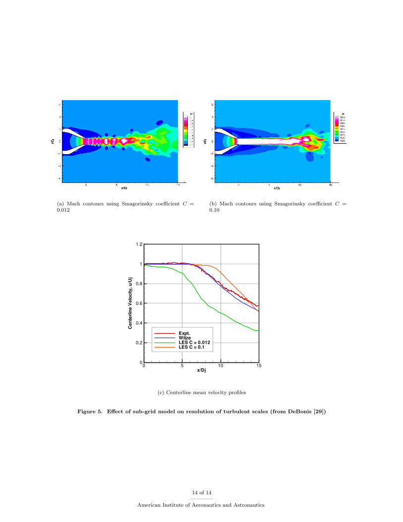
(a) Mach contours using Smagorinsky coefficient C =0.012

(b) Mach contours using Smagorinsky coefficient C =0.10

x/Dj

Cen

terli

neV

eloc

ity,u

/Uj

0 5 10 150

0.2

0.4

0.6

0.8

1

1.2

Expt.WitzeLES C = 0.012LES C = 0.1

(c) Centerline mean velocity profiles

Figure 5. Effect of sub-grid model on resolution of turbulent scales (from DeBonis [29])

14 of 14


Progress Towards Large-Eddy Simulations for Prediction of ...

Documents

Transcript of Progress Towards Large-Eddy Simulations for Prediction of ...