NASA/CR-2001-211032

Young-Person's GuideSimulation Grids

to Detached-Eddy

Philippe R. Spalart

Boeing Commercial Airplanes, Seattle, Washington

July 2001

https://ntrs.nasa.gov/search.jsp?R=20010080473 2018-05-18T20:30:46+00:00Z

The NASA STI Program Office ... in Profile

Since its founding, NASA has been dedicated

to the advancement of aeronautics and spacescience. The NASA Scientific and Technical

Information (STI) Program Office plays a key

part in helping NASA maintain this importantrole.

The NASA STI Program Office is operated byLangley Research Center, the lead center forNASA's scientific and technical information.

The NASA STI Program Office provides

access to the NASA STI Database, the largest

collection of aeronautical and space scienceSTI in the world. The Program Office is alsoNASA's institutional mechanism for

disseminating the results of its research and

development activities. These results are

published by NASA in the NASA STI Report

Series, which includes the following report

types:

TECHNICAL PUBLICATION. Reports

of completed research or a major

significant phase of research thatpresent the results of NASA programsand include extensive data or theoretical

analysis. Includes compilations ofsignificant scientific and technical dataand information deemed to be of

continuing reference value. NASAcounterpart of peer-reviewed formal

professional papers, but having less

stringent limitations on manuscript

length and extent of graphic

presentations.

TECHNICAL MEMORANDUM.

Scientific and technical findings that are

preliminary or of specialized interest,

e.g., quick release reports, workingpapers, and bibliographies that containminimal annotation. Does not contain

extensive analysis.

CONTRACTOR REPORT. Scientific and

technical findings by NASA-sponsored

contractors and grantees.

CONFERENCE PUBLICATION.

Collected papers from scientific and

technical conferences, symposia,seminars, or other meetings sponsored

or co-sponsored by NASA.

SPECIAL PUBLICATION. Scientific,

technical, or historical information from

NASA programs, projects, and missions,

often concerned with subjects having

substantial public interest.

TECHNICAL TRANSLATION. English-language translations of foreignscientific and technical material

pertinent to NASA's mission.

Specialized services that complement the

STI Program Office's diverse offeringsinclude creating custom thesauri, building

customized databases, organizing and

publishing research results ... even

providing videos.

For more information about the NASA STI

Program Office, see the following:

• Access the NASA STI Program Home

Page at http://www.sti.nasa.gov

• E-mail your question via the Internet to

help@sti.nasa.gov

• Fax your question to the NASA STI

Help Desk at (301) 621-0134

• Phone the NASA STI Help Desk at (301)621-0390

Write to:

NASA STI Help DeskNASA Center for AeroSpace Information7121 Standard Drive

Hanover, MD 21076-1320

NASA/CR-2001-211032

Young-Person's GuideSimulation Grids

to Detached-Eddy

Philippe R. Spalart

Boeing Commercial Airplanes, Seattle, Washington

National Aeronautics and

Space Administration

Langley Research Center

Hampton, Virginia 23681-2199

Prepared for Langley Research Centerunder Contract NAS1-97040

July 2001

Available from:

NASA Center for AeroSpace Information (CASI)

7121 Standard Drive

Hanover, MD 21076-1320

(301) 621-0390

National Teclmical Information Service (NTIS)

5285 Port Royal Road

Springfield, VA 22161-2171

(703) 605-6000

Young-Person's Guide to

Detached-Eddy Simulation Grids

Philippe R. Spalart

Boeing Commercial Airplanes

Abstract

We give the "philosophy", fairly complete instructions, a sketch

and examples of creating Detached-Eddy Simulation (DES) grids froin

simple to elaborate, with a priority on external flows. Although DES

is not a zonal method, flow regions with widely different gridding

requirements emerge, and should be accommodated as far as possible

if a good use of grid points is to be made. This is not unique to DES.

We brush on the time-step choice, on simple pitfalls, and on tools toestimate whether a simulation is well resolved.

1 Background

DES is a recent approach, which claims wide application, either in its initial

form [1] or in "cousins" which we define as: hybrids of Reynolds-Averaged

Navier-Stokes (RANS) and Large-Eddy Simulation (LES), aimed at high-

Reynolds-number separated flows [2, 3]. The DES user and experience base

are narrow as of 2001. The team in Renton and St Petersburg has been

exercising DES for about three years [1, 4, 5]; several groups have joined and

provided independent coding and validation [6, 7, 8]. The best reason for

confidence in DES on a quantitative basis is the cylinder paper of Travin et

al. [4], which also gives the more thoughtful definition of DES, as well as the

gridding policy which was applied. The earlier NACA 0012 paper of Shur et

al. [5] was also very encouraging, but it lacked grid refinement or even much

grid design, and tended to test the RANS and LES modes of DES separately.

Gridding is already not easy, in RANS or in LES. DES compounds the

difficulty by, first, incorporating both types of turbulence treatment in the

samefield and, second,beingdirected at complexgeometries.In fact a pure-LES grid for theseflows with turbulent boundary layers would be at leastaschallenging;fortunately, there is no usefor sucha grid in the near future,as the simulation would exceedthe current computing power by orders ofmagnitude [1].

The target flows are much too complex, no matter how simple the ge-ometry, to provide exact solutionswith which to calibrate, or evento allowexperimentssogoodthat approachingtheir resultsis anunquestionablemea-sureof success.The inertial rangeand the log layer providedvalid tests, butonly of the LESmode. Besides,manysourcesof error arepresentin the sim-ulations and may compensateeachother, sothat reducing oneerror sourcecan worsen the final answer. Here we are thinking of disagreements in the

5 to 10% range. Of course, reducing the discrepancy from say 40% to 10%

is meaningful; it is the step from 4% to 1% which is difficult to establish

beyond doubt.

For these reasons, gridding guidelines will be based on physical and nu-

merical arguments, rather than on demonstrations of convergence to a _right"

answer. Grid convergence in LES is more subtle, or confusing, than grid con-

vergence in DNS or RANS because in LES the variables are filtered quanti-

ties, and therefore the Partial Differential Equation itself depends on the grid

spacing. The order of accuracy depends on the quantity (order of derivative,

inclusion of sub-grid-scale contribution), even without walls, and the situa-

tion with walls is murky except of course in the DNS limit. We do aim at

grid convergence for Reynolds-averaged quantities and spectra, but the sen-

sitivity to initial conditions is much too strong to expect grid convergence of

instantaneous fields (except for short times with closely defined initial con-

ditions). In DES, we are not in a position to predict an order of accuracy

when walls are involved; we cannot even produce the filtered equation that

is being approximated. We can only offer the obvious statement that %he

full flow field is filtered, with a length scale proportional to A, which is the

DES measure of grid spacing". This probably applies to any LES with wall

modeling. Nevertheless, grid refinement is an essential tool to explore the

soundness of this or any numerical approach.

The guidelines below will appear daunting, with many regions that are

difficult to conceptualize at first. The most-desirable features of these grids

appear incompatible with a single structured block, and are difficult to ac-

comodate especially in 3D. This can make DES appear too heavy. We must

keep in mind that the approach shown here and fully implemented on the

tilt-rotor airfoil below is the most elaborate,andhasevolvedoveryears. Fineresultshavebeenobtained with simplergrids, howeverthe accuracywasnotquite as goodas the numberof points shouldhaveallowed.

Another limitation of this write-up is that automatic grid adaptation isnot discussed.While adaptation holds the future, combining it with LES orDES is a new field of study. On the other hand, the discussionis not limitedto DES basedon the Spalart-Allmaras (S-A) model [9]; the only impact ofusinganothermodel couldbe in the viscousspacingAy+ at the wall (§2.3.1)

and possibly issues at the boundary-layer edge (§2.3.2).

We note in passing that the "ofi3cial" value for the CDES constant (for

the S-A base model), namely 0.65, is open to revisions. DES is not very

sensitive to it, which is favorable. Several partners have had better results

with values as low as 0.25, or even 0.1. Here, "better" is largely a visual im-

pression: smaller eddies, without blow-up. In some cases, the improvement

could be that the simulation now sustains unsteadiness instead of damp-

ing it out. Using this kind of qualitative criterion is the state of the art,

in DES and generally in LES. Spectra do illustrate the improved accuracy

from lowered dissipation in a more quantitative manner [9]. We attribute

the variations in the preferred value of _Es to differences in numerical

dissipation. The simulation that led to 0.65 [5] used high-order centered

differences, whereas the ones that fit well with lower values use upwind dif-

ferences, some of them as low as second-order upwind. They may well remain

stable (meaning: suppress singular vortex stretching, which is physical, as

well as numerical instabilities) without any molecular or eddy viscosity in

the LES regions, making them essentially MILES (Monotonically Integrated

LES) there. However, MILES as it stands is ineffective in the boundary layer

(BL), and the simulations discussed here are not MILES overall.

Section 2 follows with guidelines, terminology, and comments, while §3 is

about pitfalls and §4 gives examples.

2 Guidelines

2.1 Terminology

The terms Euler Region, RANS Region, and LES Region will be introduced

one by one, along with Viscous Region, Outer Region, Focus Region and

Departure Region. The first three can be seen as parent- or "super-regions",

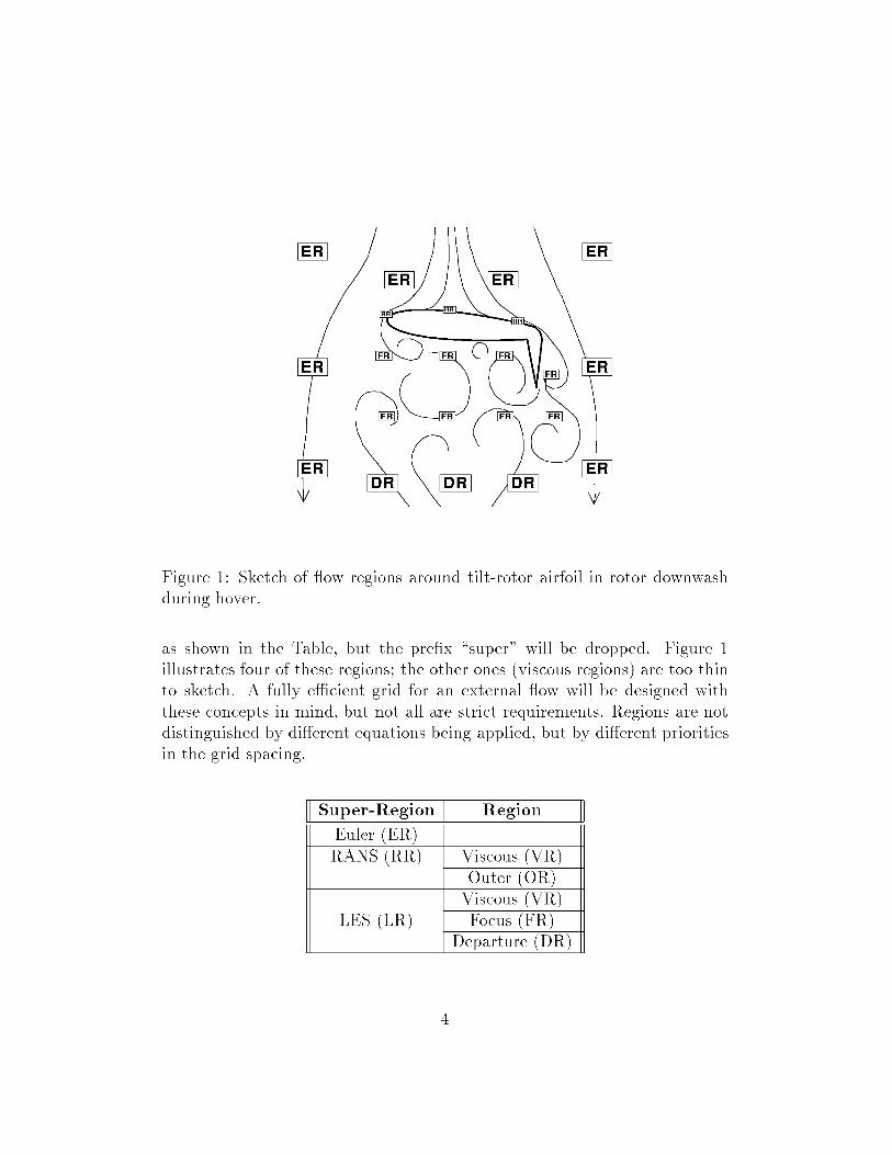
Figure 1: Sketchof flow regionsaround tilt-rotor airfoil in rotor downwashduring hover.

as shown in the Table, but the prefix "super" will be dropped. Figure 1illustrates four of theseregions;the other ones(viscousregions)are too thinto sketch. A fully efficient grid for an external flow will be designedwiththeseconceptsin mind, but not all are strict requirements.Regionsarenotdistinguishedby differentequationsbeing applied, but by different prioritiesin the grid spacing.

Super-Region RegionEuler (ER)RANS(RR)

LES(LR)

Viscous (VR)Outer (OR)

Viscous (VR)Focus (FR)

Departure (DR)

4

2.2 Euler Region (ER)

This region upstream and to the sides is never entered by turbulence, or by

vorticity except if it is generated by shocks. It extends to infinity and covers

most of the volume, but contains a small share of the grid points. The ER

concept also applies to a RANS calculation. Euler gridding practices prevail,

with fairly isotropic spacing in the three directions, and that spacing dictated

by geometry and shocks. In an ideal adapted grid, the spacing normal to the

shock would be refined, but we assume shock capturing. With structured

and especially C grids, there is a tendency for needlessly fine grid spacings

to propagate from the viscous regions into the ER, which is inefficient. This

is mitigated by taking advantage of unstructured or multiblock capabilities.

2.3 RANS Region (RR)

This is primarily the boundary layer, including the initial separation and

also any shallow separation bubbles such as at the foot of a shock. We are

assuming gridding practices typical of pure-RANS calculations. Refinement

to much finer grids would activate LES in these regions, but here we are

considering "natural" DES applications. The VR and OR overlap in the log

layer.

2.3.1 Viscous Region (VR)

This region is within the RANS region of a DES, and the requirements are

the same as for a full-domain RANS. In the wall-normal direction, DES

will create the standard viscous sublayer, buffer layer, and log layer. All

are "modeled" in the sense that the time-dependence is weak (the resolved

frequencies are much smaller than the shear rate), and does not supply any

significant Reynolds stress. The first spacing is as dictated by the RANS

model, about Ay+ = 2 or less for S-A. The stretching ratio Ayj+l/Ayj should

be in the neighborhood of 1.25 or less for the log layer to be accurate [3].

Because of this, increasing the Reynolds number by a factor of 10 requires

adding about 11 to 13 grid layers [7]. For a first attempt at a problem,

y+ _ 5 and ratio _ 1.3 should be good enough. Refinement can be done

by the usual reduction of the first step and of the stretching ratio. However

very little is typically gained by going below Ay+ = 1 and Ayj+l/Ayj = 1.2,

and in most of our studies the wall-normal spacing has been left unchanged,

and refinementhas taken placeprimarily in the LES region.In the directionsparallel to the wall, RANSpracticesarealsoappropriate.

The spacingscaleswith the steepnessof variationsof the geometryandof thecompressibleflowoutside,asundershocks.Thereis little reasonwhy it woulddiffer from the Euler spacingdiscussedabove,exceptat surfacesingularitiessuchas steps, or the trailing edge. The spacingis not constrainedin wallunits: Ax + is unlimited. Refinement will be manual and follow a scrutiny of

the solution, or be adaptive and follow standard detectors.

2.3.2 RANS outer region (OR)

The whole BL is treated with modeled turbulence, with no "LES content"

(unsteady 3D eddies). In attached BL's, a structured grid is efficient, and

the wall-parallel spacing makes the same requirements across the BL (unless

there are singular wall features such as steps, slots, or breaks in slope or

curvature).

The grid normal to the wall again follows RANS practices with the spac-

ing, ideally, nowhere exceeding about 8/10 where 8 is the BL thickness. Since

sustained stretching at the 1.25 ratio gives Ayj/yj _ log(1.25), this implies

that the stretching stops around y = 8/2. The velocity profile tolerates con-

tinued stretching to Ay = 81og(1.25) at the BL edge quite well, but the eddy

viscosity has much steeper variations in the outer layer of the BL. These vari-

ations are just as steep as near the wall, which is not needed from a physical

point of view but is a side-effect of the only practical way we have to deal with

the turbulence-freestream interface (the eddy viscosity needs to fall back to

near 0, and its behavior with k-e is very similar to that with S-A). Sharply

resolving the slope break of the S-A eddy viscosity at the BL edge has no

physical merit [10]; the concern is more over numerical robustness and mak-

ing sure that the solution inside the BL does not "feel" the edge grid spacing.

In practice, it is safer to over-estimate _ than to under-estimate it, so that

the OR often extends into the Euler Region some, and the _/10 bound is

routinely exceeded. The solver needs to tolerate the slope discontinuity and

not generate negative values.

2.4 LES regions (LR)

These regions will contain vorticity and turbulence at some point in the

simulation but are neither BL's, nor thin shear layers along which the grid

canbe aligned (suchasthe slat wakeovera high-lift airfoil).

2.4.1 Viscous region (VR)

The requirementsare the sameasin the viscousregionof the RANS region,§2.3.1. Again, even though this layer is within the LES region, the wall

spacing parallel to the wall is unlimited in wall units. We used values as high

as Ax + = Az + = 8,000 in a channel, whereas typical limits when they exist

are of the order of 20 [7].

2.4.2 Focus region (FR) and departure region (DR)

We start by setting a target grid spacing A0 that should prevail over the

"focus region" (FR), which is the region close to the body where the separated

turbulence must be well resolved. Refer again to fig. 1. A0 is the principal

measure of spatial resolution in a DES. Now we do not propagate the A0

spacing very far downstream, and so we need to decide how far downstream

the FR extends, and where the "departure region" (DR) can start. In the

DR, we are not aiming at the same resolution quality any more, and A

will eventually far exceed A0. It is a good use of grid points to have quite

different grid spacings in the two regions (once we have a sensible estimate

of where they lie), but to do this with some smoothness. If we have a single

body, and are primarily interested in forces on it, the FR can be roughly

defined by "can a particle return from this point to very near the body?".

Even more roughly, it would be "is there flow reversal at this point, at any

time?". If we have several bodies of interest, such as a wing with spoilers up

and a tail that is buffeted by the turbulence they create, the FR covers the

whole streamtube from spoilers to tail. The question became "can a particle

propagate from this point to an important flow region?" The system of two

race cars also comes to mind. If we are looking at jet noise, the FR covers

the region that generates significant noise, and the DR starts later, maybe

at 30 nozzle diameters. Laterally, the FR may well coincide with the region

enclosed inside the Ffowcs-Williams-Hawkings or Kirchhoff surface (as may

be used to extract far-field noise). These enclose all of the turbulence, with

some margin. For this flow, which is slender in the mean, ending the FR with

a DR or with an outflow condition may not make much difference. Outlining

the FR, the DR and the ER are the principal tasks in a thorough grid design,

other than setting A0. Of course, the FR is made to extend a little farther

7

than strictly necessaryfor safety.The DR may smoothly evolveto spacingssimilar to thoseof the ER. It is

a beauty and a dangerof DES that it is robust to grid spacingsthat are toocoarsefor accuracy.As the grid coarsens,the DES length scaleJ grows, the

destruction terms subsides, and the eddy viscosity grows [1]. The medium-

and far-field DR may well turn into a quasi-steady RANS (the grid spacing

can rise faster than the mixing length naturally does, and the destruction

term becomes negligible). Essentially, results in the DR will not be used; its

function is to provide the FR with a decent "neighbor" in terms of large-scale

inviscid dynamics, better than an outflow condition could and at a modest

cost.

We return to the FR, to advocate very similar grid spacings in the three

directions. Since in DES we have A = max(Ax, Ay, Az), the least expensive

way to obtain the desired A0 is to have cubic grid cells. This is the formulaic

argument. The numerical argument is that the eddy viscosity will tend to

allow steepening to about the same minimum length scale in all directions,

statistically (this is away from walls, of course). As a result, finer spacing

in one or even two directions direction is wasted. The physical argument for

cubic cells is that the premise of LES is to filter out only eddies that are small

enough to be products of the energy cascade, and therefore to be statistically

isotropic. Then, equal resolution capability in all directions is logical.

There is no unique way to choose A0. The ideal DES study contains

results with a A0, and with A0/2 (at times Rule Number 1 of DES appears

to be: "Any unsatisfactory result reported to the author is due to the user's

failure to run on a fine enough grid"). The cost ratio between the two runs is

an order of magnitude. Still, we can provide gross figures. LES is supposed

to resolve a wide range of scales, and so a l_inil_mm of 323 would appear to

be required to cover the FR in any plausible DES, in the easiest case when

the FR is roughly spherical. If it is elongated or if the geometry has fea-

tures tangibly smaller than the diameter of the FR, even the bare l_inil_mm

increases considerably. Once we add the ER, RR and DR, it is clear that

the minimum DES worth running includes well over 100,000 grid points (this

is over a geometry, as opposed to homogeneous or channel turbulence). We

have run from 200,000 to 2,500,000 [4, 5, 11] and expect simulations well

beyond 107 points in the near future.

2.5 Grey regions

There are intermediate zones between all regions. Most often, the boundaries

are not sharp, but some are, when they correspond to block boundaries. For

instance, over an airfoil we have started using a larger spanwise grid spacing

Az in the ER and DR blocks than in the RR and FR blocks, thus saving

points.

The boundary between the ER and any other region is placed within areas

that will never see vorticity, turbulence, or fine scales of motion. The grid

spacing may change quite a bit across that boundary, especially between FR

and ER or if the RR is tight around the BL. This is also typical of RANS

grids today: even within a block, the BL and ER spacings are often designed

by different algorithms. Already, these calculations have an RR and an ER.

The "hand-over" from FR to DR (recall that fluid normally does not flow

from the DR to the FR) can involve a sizeable coarsening in all directions.

We are much less invested in the DR flow physics, and the eddy viscosity

will keep the simulation stable in the DR. The same goes for any RR-to-DR

boundary. This one is present in simple RANS solutions. Often, the wake

region of a wing could fairly be described as "DR" in the sense that the grid

is unable to support the wake with its accurate thickness (even a grid cut

with fine spacing normal to the flow has no reason to be on the final position

of the wake). The viscous physics are neglected. None of these zones pose

serious physical issues.

The RR-to-FR zone or "grey area" has always been more of a concern, in

physical terms. The grid design is not troublesome. The wall-parallel spacing

has no reason to vary wildly from RR to FR (recall that the typical flow

becomes LES after separation, so that fluid goes from RR to FR). If anything,

a well-resolved FR may be finer than the RR. Normally, the separation point

is not accurately known in advance. As a result, the grid design does not

mark the RR-to-FR change much, if at all. It means the RR has more points

than needed outside the BL (as is patent in the examples below, and due

partly to structured grids), and the FR a few too many very near the wall.

The concern for this RR-to-FR zone is physical. We are expecting a

switch from 100% modeled stresses (those given by the turbulence model)

to a strong dominance of the resolved stresses (those which arise from av-

eraging an unsteady field). In other words, the RANS BL lacks any "LES

Content", and we expect a new instability, freed from the wall proximity, to

take over rapidly as the fluid pours off the surface. This possibility is more

convincingwhenseparationis from a sharpcorneror trailing edgethan froma smoothsurface.However,circular-cylinder results do not suggesta majorproblem [4]. The ultimate in difficulty may be reattachment after a largebubble. This all dependson: the thicknessand laminar/turbulent state ofthe BL; the grid spacing,which controls which wavelengthscanbe resolvedand the eddy-viscositylevel; the time step, which controls which frequenciescan be resolved;and finally (physical) global instabilities which respond toconfinementand receptivity at the separationsite. Physicsand numericsareintertwined, unfortunately.

We can only point out that no numerical treatment of separationandturbulence short of DNS will avoid thesecomplexities;that userscrutiny iskey; and that grid variation is the only coherenttool to test the sensitivityof the solutions and estimate the remaining error. Once a true DES hasbeenobtained, grid refinementhasgiven sensibleresults. The presentguideshouldprevent the cost of grid experimentationsfrom going out of control,as it would if all four directionswerevaried independentlyand blindly (as itis, the grid sizeand time stepare not tied by a very rigid rule).

Note that at separationin DES we are relying on a disparity of lengthscalesor "spectral gap" betweenthe BL turbulenceand the subsequentfree-shear-layerturbulence. This is not the sameas relying on a spectral gapover the whole separatedregion,which is the argumentneededto advocateunsteady RANS (URANS) for massiveseparation. Somegroups considerURANS asthe answerfor massively-separatedflows; we considerit as am-biguous and flawed and have consistentevidencethat its quantitative per-formancecanbe quite poor [2, 5, 4].

2.6 Time step

Here we assume that the time step is chosen for accuracy, not stability. We

primarily look at the FR, on the premise that the other regions are unlikely

to excite phenomena with higher frequency than the FR does. All the regions

(and grid blocks) run with the same time step.

We consider that a sub-grid-scale model is best adjusted to allow the en-

ergy cascade to the smallest eddies that can be safely tracked on the grid.

Therefore, eddies with wavelengths of maybe A = 5A will be active, even

though they cannot be highly accurate because they lack the energy cascade

to smaller eddies, and are under the influence of the eddy viscosity instead.

As a result, their transport by a reasonable differencing scheme (at least

10

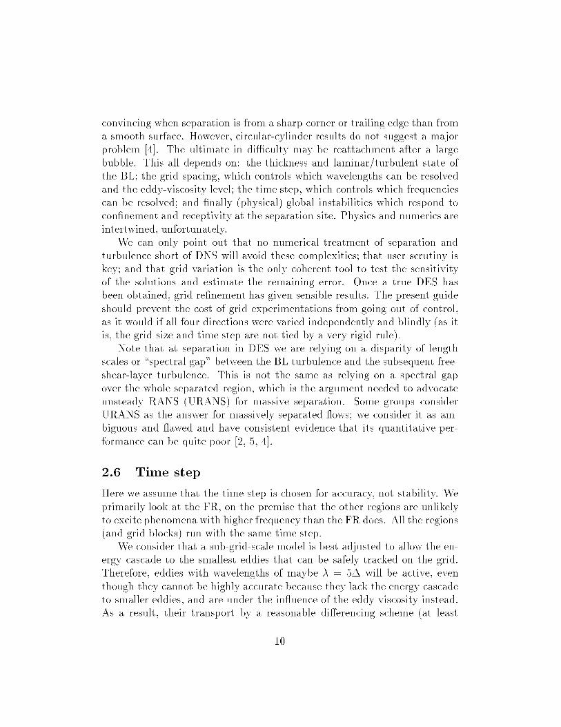
Figure 2: DES grid over NACA 0012airfoil.

second-order)with A = A/5 is acceptable, although not highly accurate. All

of this depends on the differencing scheme's performance for short waves.

To best spend the computing effort, we wish for time-integration errors that

are of the same magnitude. Again assuming a reasonable time-integration

scheme, at least second-order, we need maybe five time steps per period.

That leads to a local CFL number of 1. Again, it is based on rough accuracy

estimates, not stability. Steps a factor of 3/2 or even 2 away in either direc-

tion from this estimate cannot be described as _%correct". Unfortunately,

tests with different time steps rarely give any strong indications towards an

optimal value.

We then estimate the likely highest velocity encountered in the FR, U_n_x,

which is typically between 1.5 and several times the freestream velocity, and

arrive at the time step At = A0/U_n_x. It has been difficult to confirm or

challenge this guideline, which of course depends on the relative performance

of the spatial and temporal schemes. Orders of accuracy vary, and are of-

ten higher in the spatial directions, which would push the _%rror-balanced"

At down somewhat. All schemes of the same order are not even created

equal. Space/time error balancing is the area that leaves the most room for

experimentation.

11

3 Pitfalls

DES produces inaccurate results if the grid is too coarse or the time step too

long, just like any other numerical strategy, but rarely "blows up". The self-

adapting behavior of the eddy viscosity to the grid of course suppresses the

3D Euler singularity formation (thus removing a warning of poor resolution,

compared with DNS), but this feature is present in any LES and in many

RANS solvers so that there is no danger specific to DES. Upwind schemes,

which are common, also suppress numerical divergence. If the simulation is

grossly under-resolved, a serious step of grid refinement will trigger a large

difference, and thus alert the user (recall that a %erious step" implies a factor

of at least x/2 and therefore nearly quadruples the cost).

An issue that is specific to DES is that of "ambiguous grids". It is normal

DES practice for the user to signal the model whether RANS or Sub-Grid-

Scale (SGS) behavior is expected in a region, and DES will respond well if

the intermediate zones (in which the two branches of dare close [1]) are small

and crossed rapidly by particles. This is usually the case but in our channel

study [7], we created cases in which almost the whole domain was ambiguous.

These grids were too coarse (roughly, 5 points per channel half-height h in the

wall-parallel directions) for resolved turbulence to be sustained, so that the

solution was steady and there was no "resolved Reynolds stress". However

the turbulence model was still limited by the grid spacing in the core region;it was on the LES branch of d. The result was too little modeled stress

compared with the normal RANS level, and therefore skin friction. Themodel was confused. This was a contrived failure in the sense that these

grids were visibly too coarse, the solution obviously had none of the expected

LES content, and grid refinement would alter the results strongly enough to

prompt an investigation.

We re-iterate that strongly anisotropic grids are inefficient in the LES

region. A much finer spacing in one direction is of no value, and may fur-

thermore harm the stability of the time integration. Similarly, we need a

balance between spatial and temporal steps, a balance which is more diffi-

cult to judge than that between spatial directions. Often, two time steps

that are in a ratio of 2 appear equally sensible for the same flow on the same

grid.

A more subtle possibility is that DES would "fake" some effects that

should be properly obtained from RANS. For instance, the effects of coin-

pressibility in a mixing layer and of rotation in a vortex are to weaken the

12

15

10

2.0 y/D

1.5

1.0

0.5

0.0

-10 -5 0 5 x/DIO 15 0.0 0.5 1.0 x/D 1.52.0

Figure 3: DES grid over circular cylinder.

turbulence. RANS models calibrated in incompressible thin shear layers often

miss these effects, so that any reduction of the eddy viscosity steers results in

the desired direction. Reducing the eddy viscosity is precisely what DES does

relative to RANS, so that even a DES that lacks quality resolved turbulent

activity (for instance due to inadequate spanwise domain size or resolution)

could fortuitously improve results over RANS. Since demonstrating superi-

ority over RANS is a recurrent theme in DES papers, there is a danger of

reporting improvements, but for a wrong reason. Note that in some RANS

studies, an eddy-viscosity reduction could also compensate for numerical dis-

sipation, so that a weakened model could improve results, but then only on

coarse grids!

4 Examples

4.1 Clean airfoil over wide range of angle of attack

The grid design in our NACA 0012 study was simple, with a single block, see

Fig. 2 [5]. Compared with a RANS grid adequate for an attached case, the

13

primary differenceswere the O instead of C structure and that more pointswere placed in the FR over the upper surface. However: the ER regionunder the airfoil also had a finer grid, which wasnot needed;the FR cellswerenot all closeto cubic; no clear DR regionwasdesignedin; in particular,Az was uniform. The grid did not change with angle of attack. This was

a 141 × 61 × 25 grid with 1 chord for the spanwise period; A0 was 0.04c,

dictated by Az, and the time step At = 0.025c/U_.

4.2 Circular cylinder

The final grids for the cylinder, in addition to including refinement by a

factor of 2 in A0 from 0.068 to 0.034 diameters, have several design features

absent in the NACA-0012 grids, see Fig. 3 [4]. The ER is clearly seen; the

RR and FR are continuous; the DR is also continuous with the FR, but

the coarsening is visible. Az is uniform; the idea of coarsening z in the ER

and DR came later. Time steps ranged from 0.05 to 0.035 (the coarse-grid

step could have been higher than 0.05, but that run was inexpensive which

removed the incentive to raise At). These are longer than our CFL guideline

above (since U]n_x _ 1.5U_), partly because there are no regions with tight

curvature, and partly based on tests that showed little difference from shorter

steps.

4.3 Tilt-rotor-wing airfoil near -90 °, as in hover

In the tilt-rotor work the definitive grid has a clear ER, a C block, see Fig. 4.

The inner "snail" block, which contains the RR and part of the FR, is highly

adapted to the geometry (including the blowing slot at the flap shoulder near

(0.85,-0.1)). The first wake H block has FR character, but avoids a finely-

spaced "C-grid cut" which would have been wasteful. The evolution from

FR to DR is gradual in terms of Ax and Ay. The 2D figure of course does

not reflect the variations in Az: it is 0.03 in the RR and FR, but 0.09 in the

ER and DR blocks (the DR block with larger Az begins at y _ -2). The

time step, At = O.O15c/U, is fairly short because of the unsteady blowing

for Active Flow Control. The resolution is quite good, since the (x, y) A0

is also 0.03, with only 580,000 points total and 54 points spanwise in the

RR and FR. Although an unstructured grid could, of course, provide the

same resolution with a somewhat smaller number of grid points, the multi-

block approach is powerful (this code probably also runs faster and allows

14

higherorders of accuracythan unstructured codes). In addition, while suchextensivemulti-block grid generation is tedious, reachingthe samelevel ofcontrol in an unstructured grid would also require very numerousstepstodrive the resolution where it is desired.

4.4 Simplified landing-gear truck

The landing-gear truck of Lazos, although simplified, is the most complete

geometry treated so far [11] (although full jet-fighter configurations have been

simulated with somewhat preliminary grids but good experimental agreement

by Dr. J. Forsythe at the US Air Force Academy). The grid has thirteenblocks with an RR-FR-DR-ER structure that is not as distinct as for the

tilt-rotor, and about 2.5 million points. The compromises on structure were

forced by the complexity of the geometry, which made grid generation very

time-consuming.

5 Acknowledgements

All the present grids were generated and many ideas shaped by Drs. Hedges,

Shur, Strelets, and Travin. Drs. Squires and Forsythe took part in many

fruitful discussions. Dr. Singer reviewed the manuscript.

References

[1] P. R. Spalart, W.-H. Jou, M. Strelets and S. R. Allmaras, "Comments

on the feasibility of LES for wings, and on a hybrid RANS/LES ap-

proach". 1st AFOSR Int. Conf. on DNS/LES, Aug. 4-8, 1997, Ruston,

LA. In "Advances in DNS/LES", C. Liu and Z. Liu Eds., Greyden Press,

Columbus, OH.

[2] P. R. Spalart, "Strategies for turbulence modelling and simulations".

Int. J. Heat Fluid Flow 21, 2000, 252-263.

[3] P. R. Spalart, "Trends in turbulence treatments". AIAA-2000-2306.

[4] Travin, A., Shur, M., Strelets, M., & Spalart, P. R. 2000. "Detached-

Eddy Simulations past a Circular Cylinder". Flow, Tur'b. Comb. 63,

293-313.

15

[5]

[6]

[7]

Is]

M. Shur, P. R. Spalart, M. Strelets and A. Travin, _Detached-eddy

simulation of an airfoil at high angle of attack." 4th Int. Symposium on

Eng. Turb. Modelling and Experiments, May 24-26 1999, Corsica. W.

Rodi and D. Laurence Eds., Elsevier.

Constantinescu, G., and Squires, K. D., "LES and DES investigations

of turbulent flow over a sphere." AIAA-2000-0540.

Nikitin, N. V., Nicoud, F., Wasistho, B., Squires, K. D., & Spalart, P.

R. 2000. _An Approach to Wall Modeling in Large-Eddy Simulations".

Phys Fluids 12, 7.

Forsythe, J., Hoffmann, K., and Dieteker, J.-F., _Detached-eddy simu-

lation of a supersonic axisymmetric base flow with an unstructured flow

solver", AIAA-2000-2410.

[9] M. Strelets, _Detached eddy simulation of massively separated flows",

AIAA 2001-0879.

[10]

[11]

P. R. Spalart and S. R. Allmaras, "A one-equation turbulence model for

aerodynamic flows," La Recherche A{rospa_iale, 1, 5 (1994). Note error

in appendix for C_l.

L. S. Hedges, A. Travin & P. R. Spalart 2001. _Detached-Eddy Simula-

tions over a simplified landing gear". To be submitted, J. Fluids Er_9.

16

0.5

>-

-0.5

-!0.5 0 0.5 1

X

Figure 4: DES grid over generic tilt-rotor airfoil. Compare with fig. 1.

17

Figure 5: DES grid over landing-geartruck.

18

REPORT DOCUMENTATION PAGE Form ApprovedOMB No. 0704-0188

Public reporting burden for this collection of information is estimated to average 1 hour per response, including the time for reviewing instructions, searching existing datasources, gathering and maintaining the data needed, and completing and reviewing the collection of information. Send comments regarding this burden estimate or any otheraspect of this collection of information, including suggestions for reducing this burden, to Washington Headquarters Services, Directorate for Information Operations andReports, 1215 Jefferson Davis Highway, Suite 1204, Arlington, VA 22202-4302, and to the Office of Management and Budget, Paperwork Reduction Project (0704-0188),Washington, DC 20503.

1. AGENCY USE ONLY (Leave blank) 2. REPORT DATE 3. REPORT TYPE AND DATES COVERED

July 2001 Contractor Report

4. TITLE AND SUBTITLE

Young-Person's Guide to Detached-Eddy Simulation Grids

6. AUTHOR(S)Philippe R. Spalart

7. PERFORMING ORGANIZATION NAME(S) AND ADDRESS(ES)

Boeing Commercial AirplanesP.O. Box 3707

Seattle, WA98124

9. SPONSORING/MONITORING AGENCY NAME(S) AND ADDRESS(ES)

National Aeronautics and Space AdministrationLangley Research Center

Hampton, VA 23681-2199

5. FUNDING NUMBERS

RTR 706-81-13-02

NAS 1-97040

8. PERFORMING ORGANIZATION

REPORT NUMBER

10. SPONSORING/MONITORING

AGENCY REPORT NUMBER

NASA/CR-2001-211032

11. SUPPLEMENTARY NOTES

Prepared for Langley Research Center under Contract NAS 1-97040

Langley Technical Monitor: Craig Streett

12a. DISTRI BUTION/AVAILABILITY STATEMENT

Unclassified-Unlimited

Subject Category 64 Distribution: StandardAvailability: NASA CASI (301) 621-0390

12b. DISTRIBUTION CODE

13. ABSTRACT (Maximum 200 words)

We give the "'philosophy", fairly complete instructions, a sketch and examples of creating Detached-Eddy

Simulation (DES) grids from simple to elaborate, with a priority on external flows. Although DES is not a zonalmethod, flow regions with widely different gridding requirements emerge, and should be accommodated as far

as possible if a good use of grid points is to be made. This is not unique to DES. We brush on the time-stepchoice, on simple pitfalls, and on tools to estimate whether a simulation is well resolved.

14. SUBJECT TERMS

detached-eddy simulation, DES, large-eddy simulation, LES,

unsteady Reynolds-averaged Navier Stokes, URANS

17. SECURITY CLASSIFICATIONOF REPORT

Unclassified

18. SECURITY CLASSIFICATIONOF THIS PAGE

Unclassified

19. SECURITY CLASSIFICATIONOF ABSTRACT

Unclassified

15. NUMBER OF PAGES

2316. PRICE CODE

20. LIMITATIONOF ABSTRACT

UE

NSN 7540-01-280-5500 Standard Form 298 (Rev. 2-89)

Prescribed by ANSI Std. Z-39-18298-102