Data mining in 1D: curve fitting Related material in lecture 8 on amlbook.com.

Data mining in 1D: curve fitting

Related material in lecture 8 on amlbook.com

Review: Concepts you should know for Quiz 9-4-14

Supervised learningUnsupervised learningReinforcement learningGeneralizationEin (h) and Eout (h)Hypothesis setVersion spaceMarginsSupport vectorsVC dimensionPerceptronPerceptron learning algorithmLinearly separable

Review 2: Questions about VC dimension

The VC dimension of the perceptron in 2D is 3; nevertheless, the perceptron cannot shatter 3 points in a line.

Which labelings of 3 points in a line are not linearly separable?

Is this inconsistent with VC dimension of the 2D perceptron =3? Why or Why not?

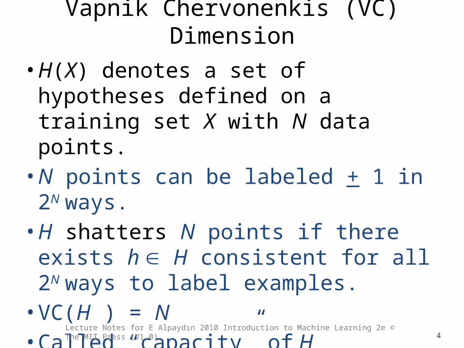
Vapnik Chervonenkis (VC) Dimension• H(X) denotes a set of hypotheses defined on

a training set X with N data points.• N points can be labeled + 1 in 2N ways.• H shatters N points if there exists h Î H

consistent for all 2N ways to label examples.• VC(H ) = N• Called “capacity” of H

4Lecture Notes for E Alpaydın 2010 Introduction to Machine Learning 2e © The MIT Press (V1.0)

Review 3: Questions about probability theory

We think of every dataset for supervised learning as being drawn from a probability distribution p(x,y) = p(x)p(y|x). What does each factor on the rhs mean?

Why is p(y|x) a factor in the probability distribution?Should we expect inputs with the same attributes to have the same labels?

“interpolation” a way to estimate values of a function from data points

Linear interpolation: connect data points by lines

Is “interpolation” a form of “data mining”?

Interpolation has a unknown “target function” f(x)

Dataset (xn, yn) is viewed as knowledge of f(x) on a finite set of points

An “hypothesis” g(x) is developed, in part, by requiring g(xn) = f(xn)

Ein(g) = 0 by construction.

More on “interpolation” as “data mining”

Eout(g) is error when hypothesis g(x) applied outside of the data set.

As always, Eout(g) cannot be calculated because f(x) is unknown outside of data.

For interpolation, “generalization” is based on continuity of f(x)

“small changes in x associated with small changes in f(x)”

Since Ein(g) =0 at data points, Eout(g) should be small when g(x) is used near a data point.

Linear interpolation has low “complexity”

Low complexity simpler implementationRequires larger data set for tight relationship between Ein(g) and Eout(g)

Linear interpolation also called “1st order spline”Higher order splines are more complex “hypothesis” in interpolation

Cubic splines: smooth interpolation

g(x), g’(x), and g”(x) continuousMore complex, harder to implementMore like target function if f ’(x),f ’’(x), etc are continuous

How interpolation differs from “real” data mining

Interpolation does not involve machine learningA single hypothesis (linear, cubic splines, etc.) is evaluatedMachine learning is finding the best hypothesis from a set H

Interpolation is deterministic because uncertainty in data is ignoredspecification of the hypothesis complete determine the result

“real” data is stochasticdrawn from unknown distribution P(x,y) = p(x)p(y|x)sometimes we think of p(y|x) as target function + noiseapplication of same data mining method to different samples of P(x,y) yields different results

Curve fitting (regression in 1D) is “real” data mining

“target function” is “trend” in the dataH in this case is the set of all 2nd degree polynomialsLess complex H (lines) obviously not adequateSelect best member of H by min sum squared residuals

Finding the best member of H by calculus

2

1

||

N

t

ttin xgrE X

Take derivatives of Ein(g) with respect to the coefficients of a parabola (collective call q ) and set equal to zero.Solve resulting 3x3 linear system

Alternatively, use a matrix method that is valid for polynomials of any degree


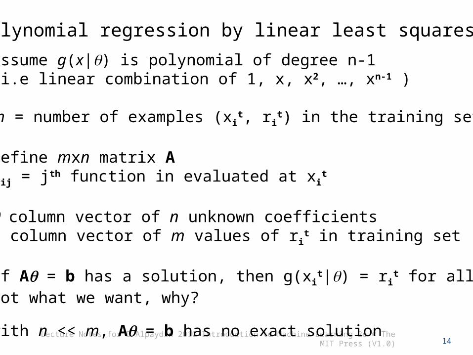
Assume g(x|q) is polynomial of degree n-1(i.e linear combination of 1, x, x2, …, xn-1 )

m = number of examples (xit, ri

t) in the training set

Define mxn matrix AAij = jth function in evaluated at xi

t

q column vector of n unknown coefficientsb column vector of m values of ri

t in training set

If Aq = b has a solution, then g(xit|q) = ri

t for all i Not what we want, why?

with n << m, Aq = b has no exact solution

Polynomial regression by linear least squares


Look for an approximate solution which minimizes the Euclidean norm of the residual vector r = b – Aq,

define f(q) = ||r||2 = rTr f(q) = (b – Aq)T(b – Aq) = bTb –2qTATb + qTATAq

A necessary condition for q0 to be minimum of f(q) is f(q0) = o

f(q) = 2ATAq – 2ATb

optimal set of parameters is a solution of nxn symmetric systemof linear equations ATAq = ATb

Normal Equations

Polynomial Regression: degree k with N data points

01

2

2012 wxwxwxwwwwwxg ttktkk

t ,,,,|

NkNNN

k

k

r

r

r

xxx

xxx

xxx

2

1

2

2222

1211

1

1

1

rD

Lecture Notes for E Alpaydın 2010 Introduction to Machine Learning 2e © The MIT Press (V1.0)

Solve DTDx = DTr for k+1 coefficients

Assignment 1: due 9/11/14

Use normal equations to fit a parabola to the data set t=linspace(0,10,21) y=[2.9, 2.7, 4.8, 5.3, 7.1, 7.6, 7.7, 7.6, 9.4, 9, 9.6,10, 10.2, 9.7, 8.3, 8.4, 9, 8.3, 6.6, 6.7, 4.1] Plot the data and the fit on the same set of axes. Show the optimum value of the parameters and calculate the sum of squared deviations between fit and data.

Review: Polynomial Regression with N points

01

2


t ,,,,|

k

1

0

2

2222

1211

w

w

w

1

1

1

Dw

kNNN

k

k

xxx

xxx

xxx

fitY


The hypothesis set with k+1 parameters is

Given the parameters that minimize the sum of squared deviations,

are the values of the fit at xt, the locations data points,and R = Yfit – Y are the residuals at the data points

Coefficient of determination


Denominator is the sum of squared error associated with the hypothesis that data is approximated by its mean value, a polynomial of degree zero

2

1

2

12|

1

N

t

t

N

t

tt

rr

xgrR

Review

1D polynomial regression (curve fitting) has all of the fundamental characteristics of data mining

• Data points (x, y) support supervised machine learning with x as the attribute and y as the label• The degree of the polynomial defines an hypothesis set• Polynomials of higher degree are more complex hypotheses.• Sum of squared residuals defines an Ein that can be used to select a member of the hypothesis set by matrix algebra.• Eout can be analytically defined and calculated for in silico datasets (target function + noise)

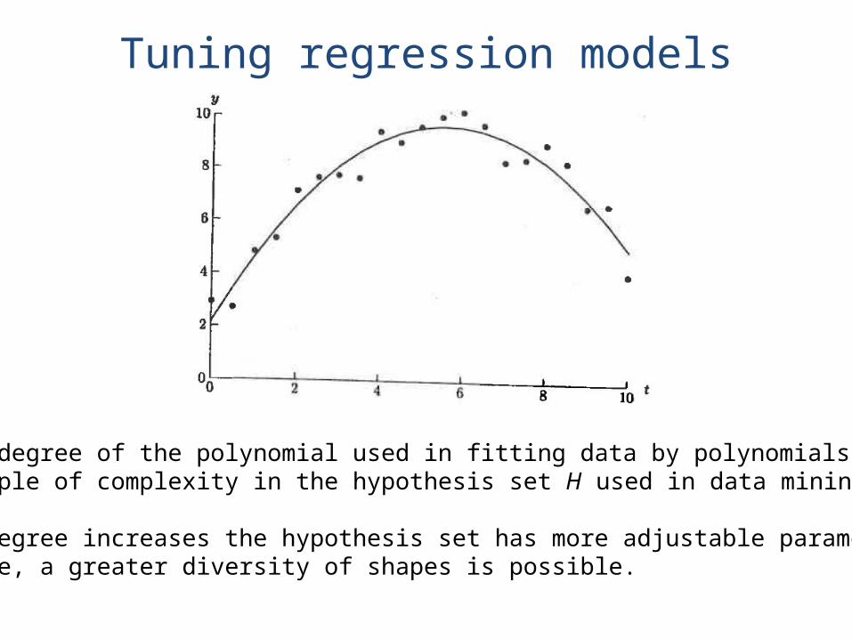
Tuning regression models

The degree of the polynomial used in fitting data by polynomials is an example of complexity in the hypothesis set H used in data mining.

As degree increases the hypothesis set has more adjustable parameters;hence, a greater diversity of shapes is possible.

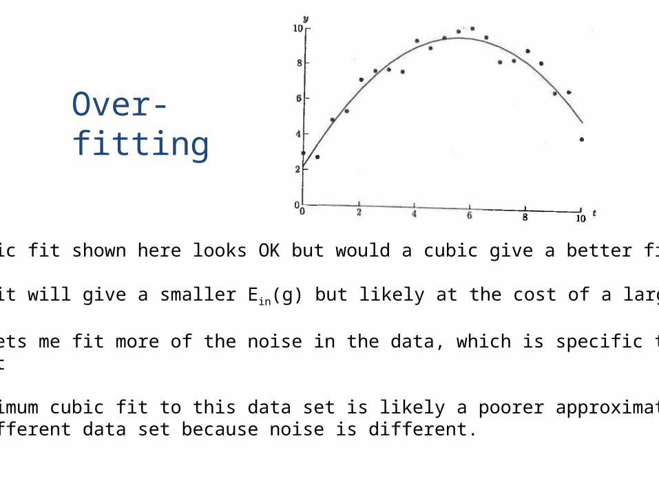
Over-fitting

Parabolic fit shown here looks OK but would a cubic give a better fit?

Cubic fit will give a smaller Ein(g) but likely at the cost of a larger Eout(g)

Cubic lets me fit more of the noise in the data, which is specific to this data set

The optimum cubic fit to this data set is likely a poorer approximation to a different data set because noise is different.

Approximation – Generalization TradeoffIn the theory of generalization (covered in lecture “feasibility of learning”) it can be shown that Eout(g) < Ein(g) + W(N, H, d) where W is a function ofN the training-set size, H the hypothesis set, and d the allowable uncertainty in the final model.

W(N, H, d) is a bound on the difference between Eout(g) and Ein(g)

If W(N, H, d) is small we can be confident of good generalization.

At given complexity (determined by H), higher statistical confidence (1-d) can usually be achieved with larger N

At fixed N and d, W usually increases with the complexity of H, making generalization less certain.

Even though Ein(g) may decrease with higher complexity, Eout(g) may not.

In least-squares 1D regression, this effect can be illustrated by the “Bias/Variance dilemma”

Fit a cubic to each of in silico data set.

Averaging these results we get a consensus cubic fit

Difference between consensus fit and target function called “bias”

From consensus fit and individual cubic fits, we can calculate a variance

Given a parabolic target function, construct several “in silico” data sets by adding noise drawn from a normal distribution with zero mean and a specified variance

Formal definitions of Bias & Variance


Assume the target function f(x) is knownCreate M in silico datasets of size N by adding noise to f(x)For each dataset find the best gi(x) of given complexityAverage gi(x) to get best overall estimator of f(x)Calculate bias and variance of best estimator as follows

2

22

1Variance

1Bias

1

t i

tti

t

tt

ti

xgxgNM

g

xfxgN

g

xgM

xg

Expectation values of Eout(g)

where < > denotes average over data sets.

Eout can be written as sum of 3 terms, s2 + bias2 + variance

where s2 is a contribution from noise in the data

s2. does not depend on complexity of the hypothesis set, so we can ignore it in this discussion


2xE| xfxgE iiout X is out-of-sample error for ith training set

Ex denotes average over the specified domain for f(x).

)(EE| 2x

2x xfxgxfxgE iiout X

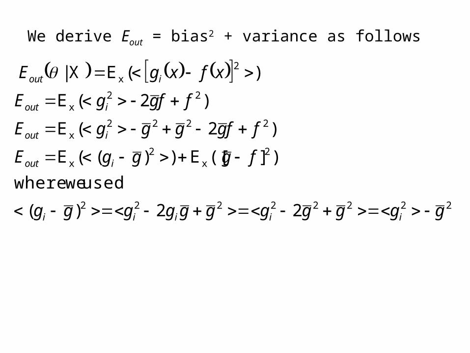
We derive Eout = bias2 + variance as follows

22222222

2x

2x

2222x

22x

2x

22)(

used wewhere

)]([E))((E

)2(E

)2(E

)(E|

ggggggggggg

fgggE

ffggggE

ffggE

xfxgE

iiiii

iout

iout

iout

iout

X

28

Bias is RMSDf

gi

g

f

one in silico experiment Linear regression: 5 experiments

Each cubic has shape like f(x) Shape of gi varies more

Polynomial fits to sin(x) + noise

Smaller Bias Larger variance

29

Best complexity is degree 3Beyond 3, decreases in bias are offset of increases in variance


Bias, variance and Eout from polynomial fits to sin(x) + noise

Cannot use bias/variance analysis to tune polynomial fits to real data because f(x) is unknown; hence we cannot calculate the bias.

Quiz #1 CS483/5809-4-14 1) How do datasets that support supervised learning, unsupervised learning and reinforcement learning differ in the label of examples? 2a) The perceptron is used as the hypothesis set for a dichotomy with classes labeled +1. What is the analytical form of h(x)?

h(x)=sign(wTx) 2b) In the model of question 2a, what does every attribute vector x have in common? x0 = 13) As a model of data with 2 attributes, the perceptron has VC dimension of 3. What does this imply for dichotomy datasets with only 3 examples?

linearly separable when they are not co-linear 4a) Define Ein(h) and Eout(h), where h is the optimum member of the hypothesis set. 4b) Explain what good generalization means in terms of Ein(h) and Eout(h).

32

“elbow” in estimate Eout indicates best complexity


divide real data into training and validation sets

Use validation set to estimate Eout

MatLab code for polynomial fitting

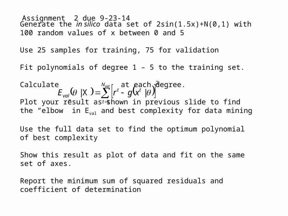
Assignment 2 due 9-23-14

Generate the in silico data set of 2sin(1.5x)+N(0,1) with 100 random values of x between 0 and 5

Use 25 samples for training, 75 for validation

Fit polynomials of degree 1 – 5 to the training set.

Calculate at each degree.

Plot your result as shown in previous slide to find the “elbow” in Eval and best complexity for data mining

Use the full data set to find the optimum polynomial of best complexity

Show this result as plot of data and fit on the same set of axes.

Report the minimum sum of squared residuals and coefficient of determination

2

1

||

valN

t

ttval xgrE X

“Elbow” suggest cubic is best complexity

Eval

Ein

Cubic fit all data: Rsq = 0.59

Is this a good fit?

Review: Polynomial Regression with N points

01

2


t ,,,,|

k

1

0

2

2222

1211

w

w

w

1

1

1

Dw

kNNN

k

k

xxx

xxx

xxx

fitY


The hypothesis set with k+1 parameters is

Given the parameters that minimize the sum of squared deviations,

are the values of the fit at xt, the locations data points,and R = Yfit – Y are the residuals at the data points

2exp

2

1 2zzp

Find a library function for random numbers drawn from p(z)

Given a random number zi from this distribution, xi = s zi + m is a random number with the desired characteristics

z is normally distributed with zero mean and unit variance

Pseudo-code for sampling a Gaussian distribution with specified mean and variance

Data mining in 1D: curve fitting Related material in lecture 8 on amlbook.com.

Documents

Transcript of Data mining in 1D: curve fitting Related material in lecture 8 on amlbook.com.