Control of Automotive Semi-Active MR Suspensions for In ...

applied sciences

Article

Control of Automotive Semi-Active MR Suspensionsfor In-Wheel Electric Vehicles

Mauricio Anaya-Martinez 1,† , Jorge-de-J. Lozoya-Santos 1,*,† , L.C. Félix-Herrán 2,† ,Juan-C. Tudon-Martinez 3,† , Ricardo-A. Ramirez-Mendoza 1,†

and Ruben Morales-Menendez 1,†

1 School of Engineering and Sciences, Tecnologico de Monterrey, Av. E Garza Sada 2501, Monterrey 64740,Mexico; [email protected] (M.A.-M.); [email protected] (R.-A.R.-M.); [email protected] (R.M.-M.)

2 School of Engineering and Sciences, Tecnologico de Monterrey Campus Sonora Norte Blvr. Enrique MazonLopez 965, Hermosillo 64849, Mexico; [email protected]

3 Engineering and Technology Faculty, Universidad de Monterrey, Av. I. Morones Prieto 4500,San Pedro Garza Garcia 66238, Mexico; [email protected]

* Correspondence: [email protected]† These authors contributed equally to this work.

Received: 27 April 2020; Accepted: 17 June 2020; Published: 29 June 2020��

Abstract: In this work, four different semi-active controllers for a quarter of vehicle and full vehiclesare evaluated and compared when used in internal combustion engine (ICE) vehicles vs electricvehicles (EVs) with in-wheel motor configuration as a way to explore the use of semi-active suspensionsystems in this kind of EVs. First, the quarter of vehicle vertical dynamics is analyzed and then afull vehicle approach explores the effectiveness of the control strategies and the effects of the tractionin the vertical Control performances. Aspects like the relation between traction and suspensionperformances, and the resonance frequencies are also discussed.

Keywords: in-wheel; semi-active; suspensions; EVs; automotive; control; switched; reluctance;motor; SR

1. Introduction

Today, automotive vehicles are considered the primary conveyance due to the high amount ofpeople, which performs its daily activities making use of them. For that, continuous improvementsfocused on safety and travel experience may be reached. During the last years, these improvementshave been devoted to enhancing automotive suspension systems, where the road holding as well as thecomfort for vehicle’s passengers have been improved. A balance between road holding and comforthas been the main goal in this area, however, most of the devoted work has been focused on internalcombustion engine vehicles. For this reason, with the high and growing adoption of the EVs, there is aneed for solutions for guaranteeing the balance between road comfort and holding especially whenworking with an in-wheel powertrain configuration with semi-active suspension systems when aswitched reluctance motor (SRM) is employed. The use of SRM instead of brushless DC (BLDC) motorsin in-wheel configurations has increased due to the low cost, efficient power transfer, high torquedensity and direct drivetrain system features that the SR motors offer for this application [1].

In the last years, some solutions in automotive suspension systems aimed to reduce vibrationeffects in in-wheel EVs have been reported. In Nagaya et al. [2], the in-wheel electric motor isemployed as an “Advanced-Dynamic-Damper-Motor” (ADM), where the electric motor is consideredas a damper mass in order to decrease tire contact force fluctuation in the vehicle. This achievementwas accomplished by attaching the motor in the unsprung mass by employing a spring and damper

Appl. Sci. 2020, 10, 4522; doi:10.3390/app10134522 www.mdpi.com/journal/applsci

http://www.mdpi.com/journal/applsci

http://www.mdpi.com

https://orcid.org/0000-0003-2538-2749

https://orcid.org/0000-0001-5536-1426

https://orcid.org/0000-0002-3243-5514

https://orcid.org/0000-0003-0646-1871

https://orcid.org/0000-0002-5122-507X

https://orcid.org/0000-0003-0498-1566

http://dx.doi.org/10.3390/app10134522

http://www.mdpi.com/journal/applsci

https://www.mdpi.com/2076-3417/10/13/4522?type=check_update&version=2

Appl. Sci. 2020, 10, 4522 2 of 28

of exclusive use, Figure 1a). As a result, the vibration of the sprung mass decreased. In Ma et al. [3],the ADM and an LQR active suspension systems are considered for sprung mass vibration reductionbut also a vertical linear force (Fv) provided by the switched reluctance (SR) in-wheel electric motor istaken into account for the analysis of the vertical dynamics. In Wang et al. [4], an FxLMS (filtered-X-leastmean square) is proposed for improving suspension performance with an active suspension system.In this case, the electric motor is considered as part of the unsprung mass, and the Fv is also consideredas an extra force adding vibration to the unsprung mass. The FxLMS controller is able to generate acontrollable force for suppressing the vibration generated by Fv. In Shao [5], the ADM complementedby an active suspension system is employed, where the suspended motor and suspension parametersare optimized based on genetic algorithms (GA) and are complemented by an LQR controller for theactive suspension system. Something similar occurs in Shao et al. [6], where the ADM is complementedby a fault-tolerant fuzzy H∞ taking into account actuator faults and control inputs restrictions.The dynamic force transmitted to the in-wheel motor is taken as an additional controlled outputas a way for reducing motor wear. In Liu et al. [7], a two-stage optimization control method isproposed to improve ADM performance. Where an LQR based on Particle Swarm Optimization (PSO)is designed for mitigating the in-wheel electric motor vibration and a finite-frequency H∞ controlleris designed for the active suspension. Obtaining, as a result, a method which is able to improve theride comfort and mitigates in-wheel motor vibration. Li et al. [8] consider the stator (housing) of thein-wheel electric motor as the unsprung mass and the rotor as an extra mass in the in-wheel vehicledynamic model, Figure 1b). In this work, a multi-objective optimization control method of activesuspension for solving the negative vibration issues generated by Fv is presented. The PSO methodis employed for obtaining active suspension system optimal parameters. The results show that theoptimized suspension system is able to reduce the effects of Fv. In Zhu et al. [1], the vibrations givenby the switched reluctance motor (SRM) are analyzed, and some control strategies which consider thevertical acceleration of the chassis as a control objective are proposed as a way of mitigating them.At the end, a switchable controller based on the proposed strategies is given as a way for guaranteeingthe best performance for each driving condition tested. As can be seen, the current work in suspensionsystems for in-wheel electric vehicles is focused on active suspension systems, which demands moreenergy consumption as well as instrumentation.

From control of semi-active suspension systems in ICE vehicles in the last years, it can besaid that the Fuzzy [9–13], Sky-Hook [14–16], and Ground-Hook [17,18] control strategies, as wellas, their variations have been the most employed techniques for satisfying the main semi-activesuspensions control objectives. In these semi-active approaches, the most common control output hasbeen the desired damping force that later is converted to current in order to manipulate the MR but insome cases, as in References [13,19], where the control output is already current. The most employedcontrol inputs are the speeds of the sprung and unsprung mass as well as the real time displacements.For the controllers validation through simulation, it is common to employ Matlab/Simulink [11–13],Carsim [19,20], Bikesim [21], Trucksim. All these programs require the parameters of the vehicle’ssuspension, and a road disturbance profile to generate results. Most of the reported results refer to timetests, where the road profile is a step or bump-like signals, and/or frequency evaluations with whitenoise or sinusoidal signals are representing the road profile. Moreover, Typically, the quantitativeperformance evaluation is performed with root mean square (RMS) values in the time domain asin Reference [9], and power spectral density (PSD) in the frequency domain [22]. For qualitativeassessments, the objective is to improve the performance achieved with a passive as much as possible.

For the experimental validation of the controller it is possible to employ an experimentalquarter of vehicle (Exp-QoV) [16], Hardware in the Loop (HiL) [23–26] or a Vehicle (Exp-V) [27],where accelerometers and sensors are employed to obtain the information that will be processed bythe controller in order to achieve the main objectives of the control strategy.

Appl. Sci. 2020, 10, 4522 3 of 28

In this work four different semi-active controllers as well as two current levels for QoVs and fullvehicles are implemented in ICE and electric vehicles with and without considering the unbalancedvertical force given by the SRM. The performances are compared as a way for visualizing how is thesuspension objectives improvement varying between the ICE and electric models. For the QoV casestudy, the simulations are carried out in MATLAB/Simulink. While for the full vehicle, software in theloop (SiL) tests are performed in MATLAB/Simulink and Carsim.

Rotor

Stator housing

ms

Kt c t

mur

Km F rZ

mus

cs

Zg

Zur

Zus

K s

Z s

a) b)

w

ms

c sKs

mu

Kt

Z s

Zus

Zr

Km

c m

mm

Figure 1. (a) Advanced-Dynamic-Damper-Motor (ADM), (b) In-wheel quarter of vehicle (QoV)three masses.

2. Methods

2.1. A Semi-Phenomenological (SP) Model of a Magnetorheological Damper

For simulation tests, a semi-phenomenological (SP) model, that comprises the hysteresis loopof the MR damper, is considered. This MR damper model was proposed in Reference [20], and itconsiders an hyperbolic tangent and the proportional effect of manipulation are employed in orderto shape the sigmoidal F−V diagram when the manipulation variable is different from 0A. This SPmodel is given by the following equations:

FD = FP(z, z, z) + FMR(z, z, I) (1)

FP = kpz + cp z + f f tanh(v f riction z + x f rictionz) (2)

FMR = CMRpost−yield Itanh× (vpre−yield z + xpre−yieldz), (3)

where FD is the MR damping force (compounded by Fp and FMR), Fp is the passive force (dampingforce when current is equal to 0A) and FMR is the force due to the magnetorheological effect of thedamper in the presence of electric current, cp is the damping coefficient, kp is the stiffness coefficient, f fis the friction coefficient, x f riction, and v f riction define the sigmoidal behavior of the friction component,xpre−yield, and vpre−yield define the sigmoidal force component due to the MR behavior and CMRpost−yieldis the damping coefficient due to the electric current. Model parameters employed for simulationpurposes are shown in Table 1.

2.2. F-Class Vehicle Model

For simulation purposes, an F-class vehicle is considered (Figure 2). F-class vehicles are known tobe vehicles with higher performance, better handling, comfort, more top quality equipment and anstupendous design. Examples of commercial vehicles classified as F-class are: Mercedes S class, Audi

Appl. Sci. 2020, 10, 4522 4 of 28

A8, and Cadillac DTS. The parameters of the F-class vehicle shown in Table 2 were extracted from theCarSim parameters library.

Table 1. Semi-Phenomenological (SP) asymmetric model parameters.

Positive Velocity, z > 0 Negative Velocity, z < 0

CMRpost−yield(NA−1) 873.9 CMRpost−yield(NA−1) 828.4vpre−yield(sm−1) 7.7 vpre−yield(sm−1) 9.6xpre−yield(m−1) 12.2 xpre−yield(m−1) 15.3

cp(Nsm−1) 530 cp(Nsm−1) 925.2kp(Nm−1) −7361.6 kp(Nm−1) −8941.1

f f (N) 115.3 f f (N) 31.7v f riction(sm−1) 32.5 v f riction(sm−1) 208.4

x f rictionm−1 66.6 x f rictionm−1 609.9

Table 2. F-class vehicle parameters in CarSim.

Variable Description Value Unit

mbs Sprung mass or body 1823 kgmus QoV unsprung mass 50 kgks f Front spring stiffness 83 N/mmksr Rear spring stiffness 44 N/mm

[z f , z f ] Suspension front stroke (jounce/rebound) +80/−60 mm[zr, zr] Suspension rear stroke (jounce/rebound) +70/−50 mm

kt Tire stiffness 230 N/mmWhbase Wheel base 3165 mm

CG Center of gravity (horizontal) 1265 mmη Motion ratio 0.614 -

ms

fd , MRKs

mu

Kt

Zs

Zus

Sprung

mass

Unsprung

mass

Zr

Figure 2. F-class vehicle, adapted from Carsim.

The main parameters of the QoV are the sprung mass (ms), which corresponds to the vehiclechassis (body) and components supported by the suspension, and the unsprung mass (mus) iscompounded by the wheel components (tire, rim, and links). From the sprung mass of the wholevehicle (mbs), the (ms) for the QoV must be estimated by making use of the weight distributionof the vehicle; which can be computed employing the dimensions shown in Figure 3. For thepresent case study, the sprung mass for the QoV is calculated as follows: mbs ∗ [1− CG/Wheelbase] =

mbs ∗ (1− 1265/3165) = mbs ∗ 0.6. For that, it can be considered that the 60% of the body mass islocated at the front part of the vehicle and 40% in the rear part.

Knowing that and considering an uniform distribution of the weight at the front (both corners)with two front passengers as well as a mid-level fuel tank, it is possible to estimate the QoV parametersshown in Table 3 for one corner of the F-class vehicle at the front, where kt represents the tire stiffnesswhich is assumed to be linked to the road (zr), and the damping effect due the tire is not considered.

Appl. Sci. 2020, 10, 4522 5 of 28

A modified F-class vehicle model is also studied, where an in-wheel electric motor is consideredinside each wheel hub instead of a unique internal combustion motor. The parameters in Table 4 areestimated knowing the new mass values, battery bank, and the characteristics of the electric motorstaken from Reference [28] (for a general), and from Reference [29] (characterized for a Brabus Electric4WD Mercedes). The modified QoV parameters are shown in Table 5. The fms and fmus resonancefrequencies were estimated according to Reference [20]. For the in-wheel electric vehicle, a residualvertical force due to the electric motor can be considered for some tests. In this case, the residualvertical force that will be considered is shown in Figure 4 as in Reference [4]. Where it was estimatedconsidering constant speed (60 km/h) and an SRM of 6 poles. The unbalanced vertical force Fv

is generated by the rotor eccentricity in the SRM and depends on the electromagnetic excitation.The unbalanced vertical force affects the vertical dynamics as an inertial force and occurs due to thegap shown in Figure 5. Which is given by the fabrication tolerances. As can be seen in Figure 5, Fv hastwo components, the radial and tangential forces (Fr and Ft).

Front

14

75

mm

1265 mm

589 mm

345mm

3165 mm

4450 mm

345mm500 m

ms

fd

, MR

Ks

mu

Kt

Zs

Zus

Sprung

mass

Unsprung

mass

Figure 3. F-class vehicle physical dimensions.

Table 3. Front QoV parameters.

Components of Quarter of Vehicle Value Units

Sprung mass (ms) 546.5 KgUnsprung mass (mus) 50 KgSpring stiffness (ks) 83 kN/m

Tire stiffness (kt) 230 kN/mms resonance frequency ( fms ) 1.2 Hz

mus resonance frequency ( fmus ) 11.5 Hz

Table 4. Modified F-class vehicle parameters in CarSim.

Variable Description Value Unit

mbs Sprung mass or body 2156 kgmus QoV unsprung mass 85 kgks f Front spring stiffness 83 N/mmksr Rear spring stiffness 44 N/mm

[z f , z f ] Suspension front stroke (jounce/rebound) +80/−60 mm[zr, zr] Suspension rear stroke (jounce/rebound) +70/−50 mm

kt All tire stiffness 230 N/mmWhbase Wheel base 3165 mm

CG Center of gravity (horizontal) 1265 mmη Motion ratio 0.614 -

Appl. Sci. 2020, 10, 4522 6 of 28

Table 5. Modified front QoV parameters.

Component of the Modified Quarter of Vehicle Value Units

Sprung mass (ms) 539 KgUnsprung mass (mus) 85 KgSpring stiffness (ks) 83 kN/m

Tire stiffness (kt) 230 kN/mms resonance frequency ( fms ) 1.13 Hz

mus resonance frequency ( fmus ) 8.76 Hz

0 0.1 0.2 0.3 0.4 0.5 0.6 0.7 0.8 0.9 1

Time (s)

0

500

1000

1500

2000

2500

3000

3500

Forc

e (N

)

Figure 4. Residual vertical force.

Figure 5. Switched reluctance motor (SRM) residual vertical force diagram, adapted from Reference [4].

2.3. QoV’s Description

The three different QoV’s—shown in Figure 6—considered for simulation purposes are describedin this section.

The normal QoV (NQoV) shown in Figure 6a corresponds to an ICE vehicle which has a semi-activesuspension system and where a sprung and an unsprung mass are considered as in Reference [30].The modified QoV (ModQoV) shown in Figure 6b corresponds to an in-wheel electric vehicleconsidering the electric motor as part of the unsprung mass and the battery bank as part of the sprungmass as it was described in Section 2.2. In Figure 6c (ModQoVFv) the same masses than in Figure 6bare considered as well as, the unbalanced vertical force (Fv) given by the in-wheel electric motor,

Appl. Sci. 2020, 10, 4522 7 of 28

as mentioned in Reference [4]. In this case, the active suspension system is replaced by a semi-activeone. The mathematical model for the NQoV and ModQoV is given by the following equations:

ms

c sKs

mu

Kt

Z s

Zus

ms

c sKs

mu

Kt

Z s

Zus

(modified)

(modified)

ms

c sKs

mu

Kt

Z s

Zus

(modified)

(modified)F

V

Zr

Zr

Zr

a) b) c)

Figure 6. QoVs for simulation, (a) NQoV, (b) ModQoV (c) ModQoVFv.

ms zs = −ks(zs − zus)− FDmus zus = −ks(zus − zs)− kt(zus − zr) + FD ,

(4)

where ms and mur are the sprung and unsprung mass, respectively. ks and kt are the stiffness of thedamper and tire, respectively. The displacements of the sprung and unsprung mass are given by zs

and zus, respectively. While the road profile is represented by zr. The damping force is given by FD,which is composed of the passive and semi-active components.

On the other hand, the mathematical model for the ModQoVFv which considers Fv is given by:

ms zs = −ks(zs − zus)− FDmus zus = −ks(zus − zs)− kt(zus − zr) + FD + Fv .

(5)

2.4. Controllers Definition

2.4.1. Sky-Hook (SH)

The SkyHook (SH) (Figure 7a) strategy is the passengers comfort analysis reference point insuspensions control due to its performance, ease of implementation and design [31]. This approachis not intended to improve road holding performance because the sprung mass vibration is notconsidered in its control law. The control system uses 2 accelerometers, and the speed and relativespeed of the sprung are usually estimated. The control law is:

c =

{cSH i f zs(zs − zus) ≥ 0

cminSH i f zs(zs − zus) < 0(6)

and the damping force (FSH) is given by:

FSH =

{cSH zs i f zs(zs − zus) ≥ 0

cminSH (zs − zus) i f zs(zs − zus) < 0(7)

where cSH y cminSH represent the damping coefficient limits (maximum and minimum, respectively),zs y zus are the sprung and unsprung mass speeds, respectively. The Sky Hook performance is limitedto low frequencies, and new improvement proposals have been proposed [31].

Appl. Sci. 2020, 10, 4522 8 of 28

2.4.2. Ground-Hook (GH)

The control strategy known as GroungHook (GH) (Figure 7b) focuses on improving the roadholding, and it is presented in Reference [18], where a fictitious element (damper) between the groundand the wheel parallel to the tire is considered. This controller follows a similar principle to the SHbut it is oriented to the dynamic tire-forces reduction to guarantee the desired level of road holding.The control law is given by:

c =

{cGH i f −zus(zs − zus) ≥ 0

cminGH i f −zus(zs − zus) < 0(8)

and the generated damping force (FGH) is given by:

FGH =

{cGH zus i f −zus(zs − zus) ≥ 0

cminGH (zs − zus) i f −zus(zs − zus) < 0(9)

ms

c (t)Ks

mu

Kt

Z s

Zus

cSH

Zr

ms

c (t)Ks

mu

Kt

Z s

Zus

cGHZ

r

a) b)

Figure 7. Heuristic controllers (a) Skyhook (b) Groundhook.

2.4.3. Mix-1-Sensor (M1S)

To reduce instrumentation costs, Savaresi and Spelta [32], developed an experiment to validatethe Mix-1 Sensor (M1S) controller performance following the SH-ADD principle employing just onesensor (suspended mass acceleration) obtaining good comfort performance. This algorithm choosesthe maximum or minimum damping coefficient at the end of each sample according to the verticalmovement of the sprung mass. The control law is:

cM1S =

{cM1S i f (z2

s − α2z2s ) ≤ 0

cminM1S i f (z2s − α2z2

s ) > 0(10)

where α is given by the masses resonance frequencies. The damping force (FM1S) is given by:

FM1S =

{cM1S zs i f (z2

s − α2z2s ) ≤ 0

cminM1S zs i f (z2s − α2z2

s ) > 0(11)

2.4.4. Frequency Estimation Based (FEB)

The Frequency Estimation Based (FEB) controller for semi-active suspensions is presentedin Reference [19]. For the manipulation signal, the harmonic motion of the damper is considered as well

Appl. Sci. 2020, 10, 4522 9 of 28

as the piston deflection, and damper deflection velocity. Displacements and speeds are approximatedemploying RMS values, and the required frequency ( f ) is estimated with:

f =

√z2

1 + z21 + ... + z2

n

(z21 + z2

2 + ... + z2n)4π2

(12)

the FEB control law is given by the following criteria:

I =

I1, i f 0 < f < f1

I2, i f f1 < f < f2

I3, i f f2 < f < f3

I4, i f f3 < f < 20

(13)

where I is the current, which will be applied to the semi-active damper. The value for I in eachinterval is chosen according to the specific requirements, for example, in a control system where themain objective is to reach both comfort and road holding requirements, the following current valuesare chosen: full current according to the damper’s operation domain (hard damping) in bandwidthintervals that contain the resonance frequencies, and 0A (soft damping) in the remaining intervals.The frequencies f1, f2 and f3 are the bandwidths limits given by:

f1 = fms +fms

2f2 = fmus −

fmus

4(14)

f3 = fmus +fmus

4(15)

the first step is to estimate the masses resonance frequencies ( fms and fms) of the QoV employing:

fms =1

2π

√kr

msfmus =

12π

√kr + kt

mus, (16)

where kr = (kw × kt)/(kw + kt) is the ride rate, kw = ks × µ2 is the wheel rate and µ is the motion ratioof the damper.

2.5. Controllers Tuning for Benchmark

Once the vehicle model is defined, the on/off controllers SH, GH, and the M1S should be tuned.This means that the ideal damping coefficients (cideal) for each controller must be approximated as it ismentioned in Reference [19]. cideal is given by Equation (17).

cideal = 2√

mkζdesired, (17)

where 2√

mk is the critical damping for the mass (m). The values of the mass (m) and stiffness (k) for thesprung mass are m = ms and k = ks, while for the unsprung mass, m = mus and k = ks ∗ kt/(ks + kt).The ideal damping force in a QoV suspension can be computed as follows:

Fideal = cideal z. (18)

By making use of the Equation (17) and QoV parameters of Tables 3 and 5 the ideal damping valuesfor a corner (front side) of the vehicle are calculated in Table 6. For the SH, GH and M1S controllers,the output signal is force, and the damper model requires electric current as input for varying theMR damping force. For force to current equivalence, a PI feedback control as in Reference [20] wasimplemented as it is shown in Figure 8. For tuning the FEB controller, four bandwidths must bedetermined according to Reference [20], and employing the resonance frequencies of the masses shownin Tables 3 and 5 for the normal and the modified QoV, respectively.

Appl. Sci. 2020, 10, 4522 10 of 28

The bandwidths for the normal and modified QoV are shown in Tables 7 and 8 respectively.In the bandwidths where the resonance frequencies are present, hard damping (2.5A) was considered,while in the rest of bandwidths, soft damping (0A) was chosen. This is the applied approach forguaranteeing a road-holding-comfort oriented suspension.

The values of 0A and 2.5A represent the minimum and the maximum current values formanipulating the MR damper, respectively. The equivalence to damping ratio is estimated accordingto the next equation.

GI =2√(k) ∗mζ

Imax ∗ CMR + cp, (19)

where GI is the desired gain of the damping value. In this case GI = 1 is considered. k andm are stiffness and mass values. From the Table 1, the values for the CMR and cp are employed.Which corresponds to the MR damper model. The equivalence current to damping ratio is presentedin Table 9.

Table 6. Values for damping coefficients computing.

Damping ζ m k cideal [Ns/m] (QoV) cideal [Ns/m] (Modified QoV)

CSH 0.6 ms η2ks 4826 4624CM1S 0.6 ms η2ks 4826 4624

CminSH 0.15 ms η2ks 1207 1155CminM1S 0.05 ms η2ks 604 550

CGH 1 musη2ks×ktη2ks+kt

7225 7706

CminGH 0.15 musη2ks×ktη2ks+kt

1206 1377

żdef

zdef

zdef

��

��

��

��

��

� �!��

�!��

��"

��#�$�"��%�

�#&��'#� ��

�#��!��

Figure 8. Force-electric current conversion with PI controller.

Table 7. Frequency Estimation Based (FEB) Frequency bandwidths for the QoV.

Road Frequency [Hz]BW1 BW2 BW3 BW4

0–1.6 1.6–8.6 8.6–14 14–20

I[A] 2.5 0 2.5 0

Table 8. FEB Frequency bandwidths for the modified QoV.

Road Frequency [Hz]BW1 BW2 BW3 BW4

0–1.7 1.7–6.6 6.6–11 11–20

I[A] 2.5 0 2.5 0

Table 9. Current to damping ratio equivalence.

Current m k ζ

0A mus η2 ks×ktks+kt

0.241.25A mus η2 ks×kt

ks+kt0.75

2.5A mus η2 ks×ktks+kt

1.26

Appl. Sci. 2020, 10, 4522 11 of 28

2.6. Input Signals Definition

The input signals definition for the time and frequency domain is done as in Reference [19].A detailed description of them is shown below.

2.6.1. Time Domain

1. Sinusoidal road with resonance frequency. As a way to visualize the comfort and road holdingconditions, whose are normally in 1–2 Hz and 10–15 Hz, a comparative work in the bodyand road holding resonance is performed employing sinusoidal roads. Two sinusoidal signalsare considered with ±10 mm and ±1 mm, respectively, Figure 9. Considering the resonancefrequency of the masses for each QoV setup.

2. Step road. A step road disturbance of magnitude 3 cm is implemented at the time of 2 s. The testduration is 4 s, Figure 9.

0 0.5 1 1.5 2 2.5 3 3.5 4

Time[s]

-0.01

-0.005

0

0.005

0.01

0.015

0.02

0.025

0.03

Road

[m]

0.01sin(2πfmst)

0.001sin(2πfmus

t)

STEP

Figure 9. Time domain input signals.

2.6.2. Frequency Domain

The evaluation of the automotive semi-active controllers with a nonlinear QoV model is madeaccording to industrial specifications [33–35]. A road drive is designed considering the shape of therelative amplitude spectrum of the position command at 10 different points between 0.1 and 30 Hz,as it is shown in Table 10. Where the 1 in amplitude relative means 15mm. This pattern was consideredin order to excite the frequencies of interest maintaining realistic velocities in the shock absorber,Figure 10 [36].

0 5 10 15 20 25 30 35

−0.012

0

0.012

Displacem

ent [m]

Time [s]

Figure 10. Frequency domain input signal.

Table 10. Definition of the relative amplitude spectrum.

Frequency [Hz] 0.1 1 2 3 4 5 8 10 20 30

Amplitude relative 1 1 0.8 0.7 0.5 0.3 0.2 0.1 0.05 0.01

2.7. Full Vehicle Tests Definition

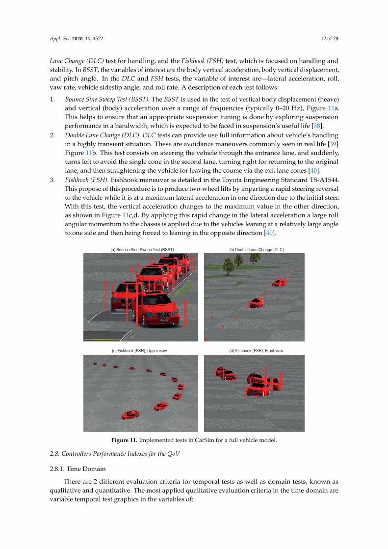
Three tests are considered for evaluating the full vehicle model in CarSim, Figure 11 [37]. The testsare—Bounce Sine Sweep Test (BSST), which is focused on ride comfort and human comfort; the Double

Appl. Sci. 2020, 10, 4522 12 of 28

Lane Change (DLC) test for handling, and the Fishhook (FSH) test, which is focused on handling andstability. In BSST, the variables of interest are the body vertical acceleration, body vertical displacement,and pitch angle. In the DLC and FSH tests, the variable of interest are—lateral acceleration, roll,yaw rate, vehicle sideslip angle, and roll rate. A description of each test follows:

1. Bounce Sine Sweep Test (BSST). The BSST is used in the test of vertical body displacement (heave)and vertical (body) acceleration over a range of frequencies (typically 0–20 Hz), Figure 11a.This helps to ensure that an appropriate suspension tuning is done by exploring suspensionperformance in a bandwidth, which is expected to be faced in suspension’s useful life [38].

2. Double Lane Change (DLC). DLC tests can provide use full information about vehicle’s handlingin a highly transient situation. These are avoidance maneuvers commonly seen in real life [39]Figure 11b. This test consists on steering the vehicle through the entrance lane, and suddenly,turns left to avoid the single cone in the second lane, turning right for returning to the originallane, and then straightening the vehicle for leaving the course via the exit lane cones [40].

3. Fishhook (FSH). Fishhook maneuver is detailed in the Toyota Engineering Standard TS-A1544.This propose of this procedure is to produce two-wheel lifts by imparting a rapid steering reversalto the vehicle while it is at a maximum lateral acceleration in one direction due to the initial steer.With this test, the vertical acceleration changes to the maximum value in the other direction,as shown in Figure 11c,d. By applying this rapid change in the lateral acceleration a large rollangular momentum to the chassis is applied due to the vehicles leaning at a relatively large angleto one side and then being forced to leaning in the opposite direction [40].

(a) Bounce Sine Sweep Test (BSST) (b) Double Lane Change (DLC)

(c) Fishhook (FSH), Upper view (d) Fishhook (FSH), Front view

Figure 11. Implemented tests in CarSim for a full vehicle model.

2.8. Controllers Performance Indexes for the QoV

2.8.1. Time Domain

There are 2 different evaluation criteria for temporal tests as well as domain tests, known asqualitative and quantitative. The most applied qualitative evaluation criteria in the time domain arevariable temporal test graphics in the variables of:

Appl. Sci. 2020, 10, 4522 13 of 28

• Sprung mass vertical acceleration. It is employed for passenger comfort analysis.• Relative displacement and/or between the two masses. It is employed the suspension

deflection analysis.• Contact force between the road profile and the wheel. It is employed for the road holding analysis.

For a quantitative evaluation, the most employed performance index is the RMS (Root MeanSquare) of the sprung mass acceleration (zs) to analyze the comfort. RMS of the unsprung massacceleration ( ¨zus) or zus− zr to analyze the road holding and RMS of the relative displacement (zs− zus)to assess suspension useful lifetime. The next equation defines the general calculation of an RMS value

RMS(x) =

√1T

∫ T

0x2dt, (20)

where x is the interest signal, and T determines the period of time during the analysis. There are somesimilar performance indexes, in Reference [9] a reduction rate of the RMS of the semi-active suspensionwith respect to the passive suspension. The equation is:

IRMS =RMSpasive − RMSsemiactive

RMSpasive, (21)

where IRMS is the variable process deviation reduction index in the time domain.

2.8.2. Frequency Domain

In the frequency domain, the PSD (power spectral density) and the pseudo-bode diagram areconsidered and described.

The performance of the semi-active suspension can be quantitatively analyzed employing PSD.Poussot-Vassal [22], determines a performance index for each control objective in terms of improving,that is to say, the semi-active system PSD is compared versus the performance of a passive suspension,employing the next equation:

IPSD =PSDpassive − PSDsemiactive

PSDpassive. (22)

Nassirharand and Taylor [41], proposed an algorithm for evaluating controllers performancein the frequency domain known as pseudo-Bode (PSB) algorithm. A pseudo-bode plot illustratesthe evaluated frequencies versus the measured gains in the transfer function. With this algorithm,it is possible to visualize the gains of the interest variables in certain frequencies in order to evaluatecomfort and road holding improvement. The PSB algorithm is given by:

1. Excite the system employing a sinusoidal signal as an input at the ϕ frequency for M periods.2. Measure the output signal zoutput (signal of interest).3. Compute the discrete Fourier transform of the input and output signal.4. Compute the magnitudes |Zr| and Zoutput.5. Compute the expression:

|G|ϕ =|Zoutput||Zr|

, (23)

where |G|ϕ is the gain to the transfer function |Zoutput ||Zr | for the given frequency ϕ.

6. The sequence must be repeated M times, each time considering a specific frequency until thedesired PSB is achieved.

Four bandwidths of interest are considered as in References [42,43] for visualizingperformance improvement.

Appl. Sci. 2020, 10, 4522 14 of 28

1. BW1: [0–2] Hz range. The main goal is comfort. The resonance frequency of the sprung mass isincluded.

2. BW2: [2–9] Hz range. The main goal is also the comfort. High gains of vertical accelerations inthis bandwidth generate overall discomfort by shaking [44].

3. BW3: [9–16] Hz range. The main goal is road holding. This bandwidth is known as tirehop BWbecause it contains the unsprung mass frequency resonance.

4. BW4: [16–20] Hz range. This will be named the head injury BW. The main goal is road holding.The dangerous vibration can generate internal damage to the body.

2.9. Controllers Performance Indexes for the Full Vehicle

For these tests, an F-class vehicle with an axis system vehicle-body-fixed system (SAE standardJ670e) is considered [45]. When working with a full vehicle, the four corners directly affect vehicle’smotion resulting on heave, pitch, roll and yaw motions. For that, suspension’s behavior of a fullvehicle model must be analyzed making use of these variables which are related to human comfort,ride comfort, road holding, vehicle handling, and vehicle roll (Table 11), [37]. The definitions of theseconcepts are:

• Human comfort is defined as the human response to vibration. Vertical acceleration of the heavein a vehicle gives the only reliable subjective-objective correlation and must be considered as theinterest value when analyzing human comfort [46].

• Ride comfort requires perfect isolation of the vehicle body from the road disturbances. To reachthe ride comfort the magnitude of the heave and pitch of the car body with respect to typical roadprofiles should be minimized [43].

• Road holding performance is the ability of a car to remain stable when moving and keep contactbetween the road and tire, especially at high speeds. It is related to the lateral acceleration.High acceleration means poor road holding [47].

• Handling is defined as the percentage of the available friction in tires or as the maximumachievable lateral acceleration employed by the car-driver combination [46]. The most typicalmeasurements are: roll, lateral acceleration, yaw rate, and vehicle sideslip angle [39,48].

• Vehicle roll is presented in the cornering, and during braking maneuvers, it can occur on perfectlysmooth roads [49]. The roll rate and roll angle of a vehicle are known as the most importantvariables when analyzing vehicle roll dynamics [50].

Table 11. Performances to be evaluated in full vehicle model tests.

Performance Interest Variables

Human comfort Body vertical accelerationRide comfort Body vertical displacement and pitch angleRoad holding Lateral acceleration

Handling Roll, yaw rate, lateral acceleration, vehicle sideslip angleRoll Roll and roll rate

2.10. Simulations and Data Processing Procedure

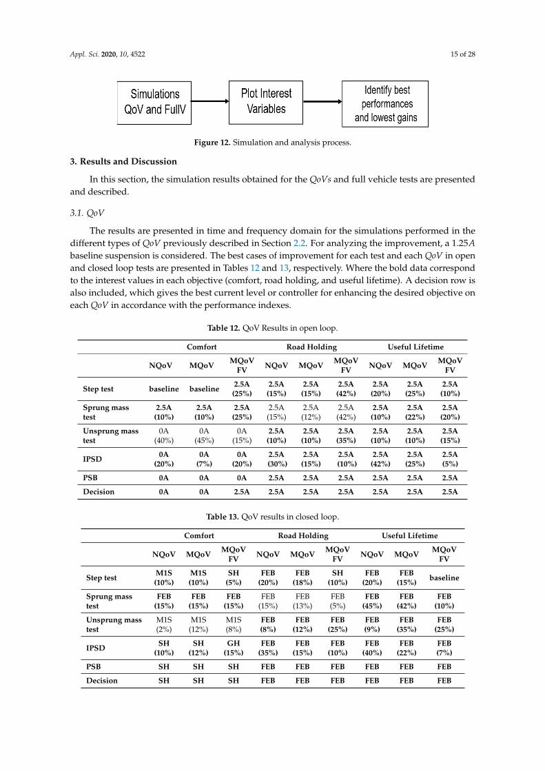
The process for simulating, processing the data and analyzing the results is summarized inFigure 12. The simulations are performed in the QoV models by varying the current levels (openloop) and control strategies (closed loop) employing the time and frequency domain input signalsdefined in Section 2.6. After that, the interest variables are processed employing the RMS and PSDalgorithms. The results are compared against the 1.25A baseline suspension. Then, the improvementsand gains are plotted and analyzed. For the full vehicle models, the simulations of the tests defined inSection 2.7 are performed employing SiL between Matlab/Simulink and Carsim. The interest variablesimprovement is visualized employing the RMS index.

Appl. Sci. 2020, 10, 4522 15 of 28

Figure 12. Simulation and analysis process.

3. Results and Discussion

In this section, the simulation results obtained for the QoVs and full vehicle tests are presentedand described.

3.1. QoV

The results are presented in time and frequency domain for the simulations performed in thedifferent types of QoV previously described in Section 2.2. For analyzing the improvement, a 1.25Abaseline suspension is considered. The best cases of improvement for each test and each QoV in openand closed loop tests are presented in Tables 12 and 13, respectively. Where the bold data correspondto the interest values in each objective (comfort, road holding, and useful lifetime). A decision row isalso included, which gives the best current level or controller for enhancing the desired objective oneach QoV in accordance with the performance indexes.

Table 12. QoV Results in open loop.

Comfort Road Holding Useful Lifetime

NQoV MQoV MQoVFV NQoV MQoV MQoV

FV NQoV MQoV MQoVFV

Step test baseline baseline 2.5A(25%)

2.5A(15%)

2.5A(15%)

2.5A(42%)

2.5A(20%)

2.5A(25%)

2.5A(10%)

Sprung masstest

2.5A(10%)

2.5A(10%)

2.5A(25%)

2.5A(15%)

2.5A(12%)

2.5A(42%)

2.5A(10%)

2.5A(22%)

2.5A(20%)

Unsprung masstest

0A(40%)

0A(45%)

0A(15%)

2.5A(10%)

2.5A(10%)

2.5A(35%)

2.5A(10%)

2.5A(10%)

2.5A(15%)

IPSD 0A(20%)

0A(7%)

0A(20%)

2.5A(30%)

2.5A(15%)

2.5A(10%)

2.5A(42%)

2.5A(25%)

2.5A(5%)

PSB 0A 0A 0A 2.5A 2.5A 2.5A 2.5A 2.5A 2.5A

Decision 0A 0A 2.5A 2.5A 2.5A 2.5A 2.5A 2.5A 2.5A

Table 13. QoV results in closed loop.

Comfort Road Holding Useful Lifetime

NQoV MQoV MQoVFV NQoV MQoV MQoV

FV NQoV MQoV MQoVFV

Step test M1S(10%)

M1S(10%)

SH(5%)

FEB(20%)

FEB(18%)

SH(10%)

FEB(20%)

FEB(15%) baseline

Sprung masstest

FEB(15%)

FEB(15%)

FEB(15%)

FEB(15%)

FEB(13%)

FEB(5%)

FEB(45%)

FEB(42%)

FEB(10%)

Unsprung masstest

M1S(2%)

M1S(12%)

M1S(8%)

FEB(8%)

FEB(12%)

FEB(25%)

FEB(9%)

FEB(35%)

FEB(25%)

IPSD SH(10%)

SH(12%)

GH(15%)

FEB(35%)

FEB(15%)

FEB(10%)

FEB(40%)

FEB(22%)

FEB(7%)

PSB SH SH SH FEB FEB FEB FEB FEB FEB

Decision SH SH SH FEB FEB FEB FEB FEB FEB

Appl. Sci. 2020, 10, 4522 16 of 28

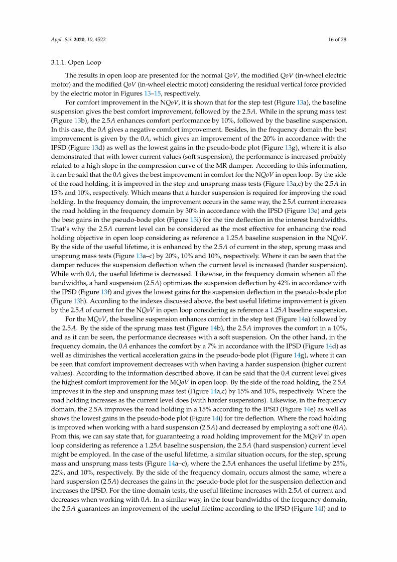
3.1.1. Open Loop

The results in open loop are presented for the normal QoV, the modified QoV (in-wheel electricmotor) and the modified QoV (in-wheel electric motor) considering the residual vertical force providedby the electric motor in Figures 13–15, respectively.

For comfort improvement in the NQoV, it is shown that for the step test (Figure 13a), the baselinesuspension gives the best comfort improvement, followed by the 2.5A. While in the sprung mass test(Figure 13b), the 2.5A enhances comfort performance by 10%, followed by the baseline suspension.In this case, the 0A gives a negative comfort improvement. Besides, in the frequency domain the bestimprovement is given by the 0A, which gives an improvement of the 20% in accordance with theIPSD (Figure 13d) as well as the lowest gains in the pseudo-bode plot (Figure 13g), where it is alsodemonstrated that with lower current values (soft suspension), the performance is increased probablyrelated to a high slope in the compression curve of the MR damper. According to this information,it can be said that the 0A gives the best improvement in comfort for the NQoV in open loop. By the sideof the road holding, it is improved in the step and unsprung mass tests (Figure 13a,c) by the 2.5A in15% and 10%, respectively. Which means that a harder suspension is required for improving the roadholding. In the frequency domain, the improvement occurs in the same way, the 2.5A current increasesthe road holding in the frequency domain by 30% in accordance with the IPSD (Figure 13e) and getsthe best gains in the pseudo-bode plot (Figure 13i) for the tire deflection in the interest bandwidths.That’s why the 2.5A current level can be considered as the most effective for enhancing the roadholding objective in open loop considering as reference a 1.25A baseline suspension in the NQoV.By the side of the useful lifetime, it is enhanced by the 2.5A of current in the step, sprung mass andunsprung mass tests (Figure 13a–c) by 20%, 10% and 10%, respectively. Where it can be seen that thedamper reduces the suspension deflection when the current level is increased (harder suspension).While with 0A, the useful lifetime is decreased. Likewise, in the frequency domain wherein all thebandwidths, a hard suspension (2.5A) optimizes the suspension deflection by 42% in accordance withthe IPSD (Figure 13f) and gives the lowest gains for the suspension deflection in the pseudo-bode plot(Figure 13h). According to the indexes discussed above, the best useful lifetime improvement is givenby the 2.5A of current for the NQoV in open loop considering as reference a 1.25A baseline suspension.

For the MQoV, the baseline suspension enhances comfort in the step test (Figure 14a) followed bythe 2.5A. By the side of the sprung mass test (Figure 14b), the 2.5A improves the comfort in a 10%,and as it can be seen, the performance decreases with a soft suspension. On the other hand, in thefrequency domain, the 0A enhances the comfort by a 7% in accordance with the IPSD (Figure 14d) aswell as diminishes the vertical acceleration gains in the pseudo-bode plot (Figure 14g), where it canbe seen that comfort improvement decreases with when having a harder suspension (higher currentvalues). According to the information described above, it can be said that the 0A current level givesthe highest comfort improvement for the MQoV in open loop. By the side of the road holding, the 2.5Aimproves it in the step and unsprung mass test (Figure 14a,c) by 15% and 10%, respectively. Where theroad holding increases as the current level does (with harder suspensions). Likewise, in the frequencydomain, the 2.5A improves the road holding in a 15% according to the IPSD (Figure 14e) as well asshows the lowest gains in the pseudo-bode plot (Figure 14i) for tire deflection. Where the road holdingis improved when working with a hard suspension (2.5A) and decreased by employing a soft one (0A).From this, we can say state that, for guaranteeing a road holding improvement for the MQoV in openloop considering as reference a 1.25A baseline suspension, the 2.5A (hard suspension) current levelmight be employed. In the case of the useful lifetime, a similar situation occurs, for the step, sprungmass and unsprung mass tests (Figure 14a–c), where the 2.5A enhances the useful lifetime by 25%,22%, and 10%, respectively. By the side of the frequency domain, occurs almost the same, where ahard suspension (2.5A) decreases the gains in the pseudo-bode plot for the suspension deflection andincreases the IPSD. For the time domain tests, the useful lifetime increases with 2.5A of current anddecreases when working with 0A. In a similar way, in the four bandwidths of the frequency domain,the 2.5A guarantees an improvement of the useful lifetime according to the IPSD (Figure 14f) and to

Appl. Sci. 2020, 10, 4522 17 of 28

the pseudo-bode gains from Figure 14h. According to the results described above, the 2.5A of current(hard suspension) guarantees the useful lifetime improvement for the MQoV in open loop consideringas reference a 1.25A baseline suspension.

Vertical Acceleration

0A 2.50ASuspension

-55

-50

-45

-40

-35

-30

-25

-20

-15

-10

-5

0

RM

S Im

pro

vem

en

t [%

]

0A 2.50ASuspension

-100

-80

-60

-40

-20

0

20

0A 2.50ASuspension

-50

-40

-30

-20

-10

0

10

0A 2.50ASuspension

-100

-80

-60

-40

-20

0

RM

S Im

pro

vem

en

t [%

]

0A 2.50ASuspension

-200

-150

-100

-50

0

0A 2.50ASuspension

-90

-80

-70

-60

-50

-40

-30

-20

-10

0

10

0A 2.50ASuspension

0

5

10

15

20

25

30

35

RM

S Im

pro

vem

en

t [%

]

0A 2.50ASuspension

-250

-200

-150

-100

-50

0

0A 2.50ASuspension

-140

-120

-100

-80

-60

-40

-20

0

Suspension deflection Suspension deflection Vertical Acceleration Suspension deflection Suspension deflection Vertical Acceleration Suspension deflection Suspension deflection

(d) Sprung mass acceleration, zsddt /z r

2WB1WBBandwidths

-30

-20

-10

0

10

20

Imp

rove

men

t [%

]

0A

2.5A

(e) Tire deflection, (zus − zr ) /z r

4WB3WBBandwidths

-40

-20

0

20

Imp

rove

men

t [%

]

0A

2.5A

(f) Suspension deflection, z/z r

BW1 BW2 BW3 BW4Bandwidths

-40

-20

0

20

40

Imp

rove

men

t [%

]

0A2.5A

2 4 6 8 10 12 14 16 18 20

frequency [Hz]

1

2

3

4

5

gai

n

0A2.5A

baseline

2 4 6 8 10 12 14 16 18 20

frequency [Hz]

1

2

3

4

5

gai

n

0Abaseline

2.5A

2 4 6 8 10 12 14 16 18 20

frequency [Hz]

50

100

150

200

250

300

350

ga

in

0A

2.5A

baseline

(h) Suspension deflection, z/z r

(i) Tire deflection, (zus − zr ) /z r

(a) Step test (b) Sprung mass resonance test (c) Unprung mass resonance test

(g) Sprung mass acceleration, zsddt /z r

Figure 13. Results from open loop simulations for the comparison in a nonlinear QoV modelconsidering a 1.25A baseline suspension.

Appl. Sci. 2020, 10, 4522 18 of 28

(a) Step test

0A 2.50ASuspension

-45

-40

-35

-30

-25

-20

-15

-10

-5

0

RM

S Im

pro

ve

me

nt

[%]

0A 2.50ASuspension

-80

-60

-40

-20

0

20

0A 2.50ASuspension

-50

-40

-30

-20

-10

0

10

(b) Sprung mass resonance test

0A 2.50ASuspension

-100

-80

-60

-40

-20

0

RM

S Im

pro

ve

me

nt

[%]

0A 2.50ASuspension

-200

-150

-100

-50

0

0A 2.50ASuspension

-90

-80

-70

-60

-50

-40

-30

-20

-10

0

10

(c) Unsprung mass resonance test

0A 2.50ASuspension

-5

0

5

10

15

20

25

30

35

40

45

RM

S Im

pro

ve

me

nt

[%]

0A 2.50ASuspension

-160

-140

-120

-100

-80

-60

-40

-20

0

20

0A 2.50ASuspension

-100

-80

-60

-40

-20

0

Vertical Acceleration Suspension deflection Suspension deflection Vertical Acceleration Suspension deflection Suspension deflection Vertical Acceleration Suspension deflection Suspension deflection

(d) Sprung mass acceleration,zs /z r

2WB1WBBandwidths

-20

-15

-10

-5

0

5

Imp

rove

me

nt

[%]

0A

2.5A


4WB3WBBandwidths

-10

-5

0

5

10

Imp

rove

me

nt

[%]

0A

2.5A

(f) Suspension deflection,z/z r


-20

-10

0

10

20

Imp

rove

me

nt

[%]

0A

2.5A

2 4 6 8 10 12 14 16 18 20

frequency [Hz]

50

100

150

200

250

300

gai

n

baseline

0A2.5A

2 4 6 8 10 12 14 16 18 20

frequency [Hz]

1

2

3

4

5

gai

n

baseline

0A2.5A

2 4 6 8 10 12 14 16 18 20

frequency [Hz]

1

2

3

4

5

gai

n

baseline

0A2.5A

(g) Sprung mass acceleration,zs /z r (h) Suspension Deflection,zdef /z r

(i) Tire Deflection, (zus − zr ) /z r

Figure 14. Results from open loop simulations for the comparison in a nonlinear modified QoV modelconsidering a 1.25A baseline suspension.

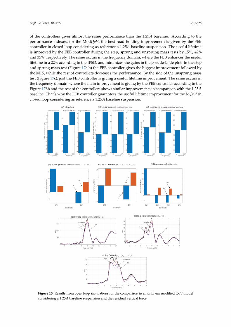
In the MQoVFV, the highest comfort improvement (25%) during the step and sprung mass tests(Figure 15a,b) is given by the 2.5A current level. In both cases, the performance decreases as well asthe current does. Besides, in the frequency domain, comfort enhancement is given in a 10% by the2.5A in accordance with the IPSD (Figure 15e) as well as with the lower gains from the pseudo-bodeplot (Figure 15g). That’s why it can be said that the 2.5A gives the best improvement for the MQoVFVin open loop is given by the 2.5A, which probably means that the presence of the unbalanced verticalforce, demands a harder suspension for improving comfort. The road holding is improved by 42% and35% in the step and sprung mass tests (Figure 15a,c), respectively. Where the road holding decreases,the current also does. In the frequency domain it occurs in almost the same way; a higher currentguarantees the road holding. The highest road holding improvement is of 10% in accordance withthe IPSD (Figure 15e) and is given by the 2.5A as well as the lowest gains for the tire deflection inthe pseudo-bode plot (Figure 15i). The 0A current level gives a negative improvement. According tothe performance discussed above, it can be said that a harder suspension (2.5A) guarantees the road

Appl. Sci. 2020, 10, 4522 19 of 28

holding in the MQoVFV in open loop. By the side of the useful lifetime the 2.5A improves it for the step,sprung mass and unsprung mass tests (Figure 15a) by 10%, 20% and 15%, respectively. Whereas inthe other QoV models, the useful lifetime increases as the current level does. In the frequency domainit occurs almost the same way; the suspension deflection is enhanced by the 2.5A in a 5% accordingto the IPSD (Figure 15f) as well as to the lower gains shown in the pseudo-bode plot (Figure 15h).As can be seen, higher current values guarantee a higher useful lifetime. The best useful lifetimeimprovement is given by the 2.5A of current for the MQoVFV in open loop considering as reference a1.25A baseline suspension.

For the comfort in the NQoV, the M1S controller enhances it during the step test (Figure 16a)by 10%. Which means that the M1S is working better during the compression of the damper. In thiscase the SH and FEB controllers decreases the comfort. While in the sprung mass test (Figure 16b),the FEB improves comfort by 15%, followed by the M1S. On the other hand, the SH controller givesthe best results in frequency domain in accordance with the IPSD (10%, Figure 16d) and with thesprung mass acceleration gains from the pseudo-bode plot (Figure 16g), while the rest of the controllersdecreases comfort. In accordance with the information analyzed above, the SH controller is givingthe best comfort enhancement for the NQoV in closed loop considering as reference a 1.25A baselinesuspension. By the side of the road holding, the GH, M1S and FEB controllers enhance the roadholding, however, the best improvement (20%) is given by the FEB controller followed by the M1S inthe step test (Figure 16a). For the unsprung mass test (Figure 16c), the FEB controller is the only onewhich improves (8%) the road holding, the rest of the controllers gives negative results. By the sideof the frequency domain, the FEB controller, shows the best performance in the interest bandwidths,in accordance with the IPSD (35%, Figure 16e) and with the pseudo-bode plot (Figure 16i). The rest ofthe controllers obtain similar results with respect to the 1.25A baseline. According to the performanceindexes discussed above, the FEB controller improves the road holding in the NQoV in closed loopconsidering as reference a 1.25A baseline suspension. For the useful lifetime in the NQoV, the FEBcontroller is the only one which gives an improvement in the time domain (Figure 16a–c) for the step(20%), sprung mass (45%), and unsprung mass tests (9%). In the frequency domain, the FEB gives thebest improvement (40%) in all the bandwidths, as well as the lowest gains according to Figure 16f,h.It can be said that the FEB controller guarantees the useful lifetime improvement for the NQoV inclosed loop considering as reference a 1.25A baseline suspension.

3.1.2. Closed Loop

The results in closed loop are presented for the normal QoV, the modified QoV (in-wheel electricmotor) and the modified QoV (in-wheel electric motor) considering the residual vertical force providedby the electric motor in Figures 16–18, respectively.

For the case of the MQoV, in the step test (Figure 17a), the M1S is the unique controller thatenhances the comfort (10%) which means that in comparison with an intermediate current value(1.25A) the M1S enhances the damping action during compression. By the case of the sprung mass test(Figure 17b), the best performance in comfort is giving by the FEB controller (15%), followed by theM1S. The rest of controllers decreases the performance. In the frequency domain, the SH controllergives a minimum improvement (12%) according to the IPSD (Figure 17d), and the pseudo-bode plot(Figure 17d), where it can be seen that the performance of the SH is similar to the 1.25A baseline, whichmeans that the baseline suspension is also a good option for improving comfort. According to theindexes discussed above, we can conclude that the SH enhances the comfort for the MQoV in closedloop considering as reference a 1.25A baseline suspension. By the side of the road holding, in the steptest (Figure 17a), FEB controller gives the highest improvement (18%) followed by the M1S and GHcontrollers. For the unsprung mass test (Figure 17c), the best road holding performance (12%) is alsogiven by the FEB controller, the rest of controllers, decreases the performance in comparison with the1.25A baseline. By the side of the frequency domain, the FEB controller provides the best improvement(15%) as well as the lowest gains in the bandwidths of interest, as it is shown in Figure 17i,e. The rest

Appl. Sci. 2020, 10, 4522 20 of 28

of the controllers gives almost the same performance than the 1.25A baseline. According to theperformance indexes, for the ModQoV, the best road holding improvement is given by the FEBcontroller in closed loop considering as reference a 1.25A baseline suspension. The useful lifetimeis improved by the FEB controller during the step, sprung and unsprung mass tests by 15%, 42%and 35%, respectively. The same occurs in the frequency domain, where the FEB enhances the usefullifetime in a 22% according to the IPSD, and minimizes the gains in the pseudo-bode plot. In the stepand sprung mass test (Figure 17a,b) the FEB controller gives the biggest improvement followed bythe M1S, while the rest of controllers decreases the performance. By the side of the unsprung masstest (Figure 17c), just the FEB controller is giving a useful lifetime improvement. The same occurs inthe frequency domain, where the main improvement is giving by the FEB controller according to theFigure 17f,h and the rest of the controllers shows similar improvements in comparison with the 1.25Abaseline. That’s why the FEB controller guarantees the useful lifetime improvement for the MQoV inclosed loop considering as reference a 1.25A baseline suspension.

(a) Step test

0A 2.50ASuspension

-30

-25

-20

-15

-10

-5

0

5

10

15

20

RM

S Im

pro

ve

me

nt

[%]

0A 2.50ASuspension

-20

-15

-10

-5

0

5

0A 2.50ASuspension

-40

-30

-20

-10

0

10

20

30

40

(b) Sprung mass resonance test

0A 2.50ASuspension

-20

-15

-10

-5

0

5

10

15

20

25

RM

S Im

pro

ve

me

nt

[%]

0A 2.50ASuspension

-15

-10

-5

0

5

10

15

0A 2.50ASuspension

-30

-20

-10

0

10

20

30

40

(c) Unsprung mass resonance test

0A 2.50ASuspension

-20

-15

-10

-5

0

5

10

RM

S Im

pro

ve

me

nt

[%]

0A 2.50ASuspension

-10

-5

0

5

10

0A 2.50ASuspension

-40

-30

-20

-10

0

10

20

30

(d) Sprung mass acceleration, zs /z r

2WB1WBBandwidths

-5

0

5

10

15

Imp

rove

me

nt

[%]

0A

2.5A


4WB3WBBandwidths

-10

-5

0

5

10

Imp

rove

me

nt

[%]

0A

2.5A

(f) Suspension deflection, z/zr


-5

0

5

10

15

20

Imp

rove

me

nt

[%]

0A

2.5A

Vertical Acceleration Suspension deflection Suspension deflection Vertical Acceleration Suspension deflection Suspension deflectionVertical Acceleration Suspension deflection Suspension deflection

2 4 6 8 10 12 14 16 18 20

frequency [Hz]

500

1000

1500

gain

2.5A

baseline0A

2 4 6 8 10 12 14 16 18 20

frequency [Hz]

2

4

6

8

10

12

14

gai

n

2.5A0A

baseline

2 4 6 8 10 12 14 16 18 20

frequency [Hz]

2

4

6

8

10

gain

0A

2.5A baseline

(g) Sprung mass acceleration,z /zr (h) Suspension Deflection,z /zrdef


Figure 15. Results from open loop simulations for the comparison in a nonlinear modified QoV modelconsidering a 1.25A baseline suspension and the residual vertical force.

Appl. Sci. 2020, 10, 4522 21 of 28

SH GH M1S FEBSuspension

-20

-15

-10

-5

0R

MS

Imp

rove

me

nt

[%]


-40

-30

-20

-10

0

10


-25

-20

-15

-10

-5

0

5

10


-50

-40

-30

-20

-10

0

10

RM

S Im

pro

vem

ent

[%]


-120

-100

-80

-60

-40

-20

0

20

40


-50

-40

-30

-20

-10

0

10


-5

-4

-3

-2

-1

0

1

RM

S Im

pro

vem

en

t [%

]


-30

-20

-10

0

10

20

30


-12

-10

-8

-6

-4

-2

0

2

4

6

8


2WB1WBBandwidths

-30

-25

-20

-15

-10

-5

0

Imp

rove

men

t [%

]

SH GH M1S

FEB

4WB3WBBandwidths

0

5

10

15

20

25

30Im

pro

vem

ent

[%]

SH GH M1S

FEB


0

10

20

30

Imp

rov

em

en

t [%

]

SH GH M1S

FEB

2 4 6 8 10 12 14 16 18 20

frequency [Hz]

50

100

150

200

250

300

350

gai

n

baseline

SH

GHFEB

M1S

2 4 6 8 10 12 14 16 18 20

frequency [Hz]

0.5

1

1.5

2

2.5

3

3.5

4

ga

in

FEBbaseline

GHM1S

SH

2 4 6 8 10 12 14 16 18 20

frequency [Hz]

0.5

1

1.5

2

2.5

3

ga

in

baseline

SH

GHFEB

M1S


(d) Sprung mass acceleration, zsddt /z r (e) Tire deflection, (zus − zr ) /z r (f) Suspension deflection, z/z r

(g) Sprung mass acceleration, zsddt /z r (h) Suspension deflection, z/z r


Figure 16. Results from closed simulations for the comparison in a nonlinear QoV model considering a1.25A baseline suspension.

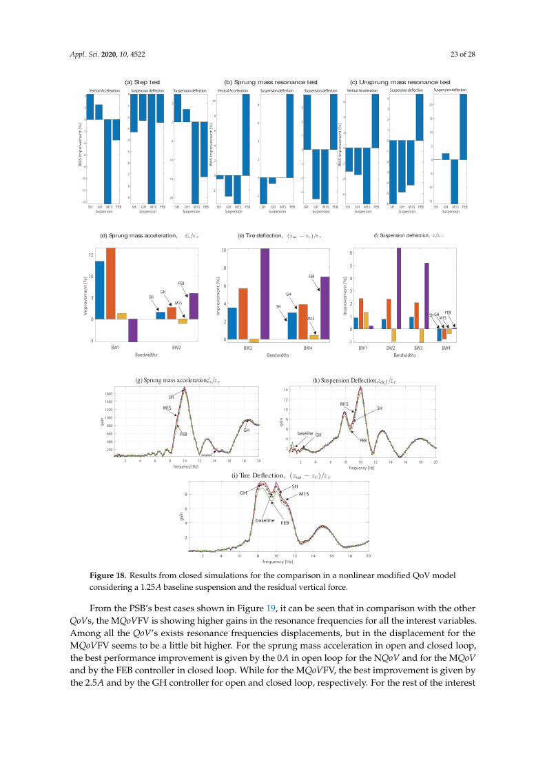
In the MQoVFV, comfort is improved in the step test (Figure 18a) by the SH controller in a 5%followed by the GH controller, the rest of the controllers gives negative improvements. Besides, in thesprung mass test (Figure 18b), the comfort is enhanced by the FEB controller by 15%. While the rest ofcontrollers shows lower improvements than the baseline suspension. On the other hand, according tothe IPSD (Figure 18a), the GH controller enhances the comfort by a 15% followed by the FEB controller.While in the pseudo-bode plot (Figure 18a), the lower gains are given by the SH controller followed bythe GH controller. According to the information described above, it can be said that the SH controllergives the highest comfort improvement for the MQoVFV in closed loop. By the side of the road holding,the SH controller enhances it by 10% during the step test (Figure 18a) followed by the GH controller.The rest of the controllers show negative improvements. While in the unsprung mass (Figure 18c),the road holding is enhanced by the FEB controller by 25%, also followed by the GH controller. In thefrequency domain occurs almost the same, the FEB followed by the GH controller enhances the tire

Appl. Sci. 2020, 10, 4522 22 of 28

deflection by 10% in accordance with the IPSD (Figure 18e) as well as gives the lowest gains in thepseudo-bode plot (Figure 18i). According to the information discussed above, the highest road holdingimprovement in the MQoVFV is given by the FEB controller in closed loop tests when comparedagainst the 1.25A baseline suspension. Finally, the useful lifetime is improved by the 1.25A baselinein the step test (Figure 18a), followed by the GH and M1S controllers. While in the sprung mass andunsprung mass tests (Figure 18b,c), the FEB controller enhances the useful lifetime in a 10% and 25%,respectively. Where the rest of the controllers shows negative improvements. The same occurs in thefrequency domain, where according to the IPSD (Figure 18f) and to the pseudo-bode plot (Figure 18h)gains, the FEB controller enhances the performance by 7%. That’s why it can be stated that the FEBcontroller gives the higher useful lifetime improvement for the MQoVFV in closed loop, which meansthat suspension deflection has been decreased by the FEB controller.


-25

-20

-15

-10

-5

0

RM

S Im

pro

vem

ent

[%]


-50

-40

-30

-20

-10

0

10


-20

-15

-10

-5

0

5

10

15


-50

-40

-30

-20

-10

0

10

RM

S Im

pro

vem

en

t [%

]


-120

-100

-80

-60

-40

-20

0

20

40


-40

-30

-20

-10

0

10


-8

-6

-4

-2

0

2

4

6

8

10

RM

S Im

pro

vem

en

t [%

]


-40

-30

-20

-10

0

10

20

30


-20

-15

-10

-5

0

5

10

2WB1WBBandwidths

-15

-10

-5

0

Imp

rove

me

nt

[%]

SH GHM1S

FEB

4WB3WBBandwidths

-2

0

2

4

6

8

10

Imp

rove

me

nt

[%]

SH GH M1S

FEB


-5

0

5

10

15

20

Imp

rove

me

nt

[%]

SH GHM1S

FEB

2 4 6 8 10 12 14 16 18 20

frequency [Hz]

50

100

150

200

250

300

gai

n

baselineFEB

M1S GH

SH

2 4 6 8 10 12 14 16 18 20

frequency [Hz]

0.5

1

1.5

2

2.5

3

3.5

4

gai

n

baseline

FEB

M1S

GH

SH

2 4 6 8 10 12 14 16 18 20

frequency [Hz]

0.5

1

1.5

2

2.5

3

3.5

4

ga

in

FEB

baseline

M1S

GH

SH



(d) Sprung mass acceleration, zsddt /z r (e) Tire deflection, (zus − zr ) /z r (f) Suspension deflection, z/z r

(g) Sprung mass acceleration, zsddt /z r (h) Suspension deflection, z/z r


Figure 17. Results from closed simulations for the comparison in a nonlinear modified QoV modelconsidering a 1.25A baseline suspension.

Appl. Sci. 2020, 10, 4522 23 of 28


-14

-12

-10

-8

-6

-4

-2

0

2

4

RM

S Im

pro

vem

ent

[%]


-9

-8

-7

-6

-5

-4

-3

-2

-1

0


-20

-15

-10

-5

0

5


-2

0

2

4

6

8

10

RM

S Im

pro

vem

en

t [%

]SH GH M1S FEB

Suspension

-2

0

2

4

6

8


-3

-2

-1

0

1

2

3


-6

-4

-2

0

2

4

6

RM

S Im

pro

vem

ent

[%]


-6

-5

-4

-3

-2

-1

0

1

2

3

4


-15

-10

-5

0

5

10

15

20

(a) Step test (b) Sprung mass resonance test (c) Unsprung mass resonance testVertical Acceleration Suspension deflection Suspension deflection Vertical Acceleration Suspension deflection Suspension deflectionVertical Acceleration Suspension deflection Suspension deflection

(d) Sprung mass acceleration, zs /z r

2WB1WBBandwidths

-5

0

5

10

15

Imp

rove

me

nt

[%]

SHGH

M1S

FEB


4WB3WBBandwidths

0

2

4

6

8

10

Imp

rov

em

en

t [%

]

SH

GH

M1S

FEB

(f) Suspension deflection, z/z r


-1

0

1

2

3

4

5

6

Imp

rove

me

nt

[%]

SHGHM1S

FEB

2 4 6 8 10 12 14 16 18 20

frequency [Hz]

200

400

600

800

1000

1200

1400

1600

gai

n

FEB

M1S

baseline

GH

SH

2 4 6 8 10 12 14 16 18 20

frequency [Hz]

2

4

6

8

10

12

14

gai

n

FEB

M1SSH

GHbaseline

2 4 6 8 10 12 14 16 18 20

frequency [Hz]

2

4

6

8

gain

FEB

M1S

SHGH

baseline

(g) Sprung mass acceleration,zs /z r (h) Suspension Deflection,zdef /z r


Figure 18. Results from closed simulations for the comparison in a nonlinear modified QoV modelconsidering a 1.25A baseline suspension and the residual vertical force.

From the PSB’s best cases shown in Figure 19, it can be seen that in comparison with the otherQoVs, the MQoVFV is showing higher gains in the resonance frequencies for all the interest variables.Among all the QoV’s exists resonance frequencies displacements, but in the displacement for theMQoVFV seems to be a little bit higher. For the sprung mass acceleration in open and closed loop,the best performance improvement is given by the 0A in open loop for the NQoV and for the MQoVand by the FEB controller in closed loop. While for the MQoVFV, the best improvement is given bythe 2.5A and by the GH controller for open and closed loop, respectively. For the rest of the interest

Appl. Sci. 2020, 10, 4522 24 of 28

variables, the best performance improvement is given by the same current and control strategy in allthe QoV’s.

(a) Sprung mass acceleration,zs /z r

2 4 6 8 10 12 14 16 18 20

frequency [Hz]

200

400

600

800

1000

1200

1400

1600

gain

2 4 6 8 10 12 14 16 18 20

frequency [Hz]

2

4

6

8

10

12

gain

(e) Tire Deflection, (zus − zr ) /z r

2 4 6 8 10 12 14 16 18 20

frequency [Hz]

1

2

3

4

5

6

7

8

gain

2.5A MQoVFV

0A MQoV 0A NQoV

2.5A MQoVFV

2.5A MQoV 2.5A NQoV

2.5A NQoV2.5A MQoV

2.5A MQoVFV

(c)Suspension Deflection, zdef /z r

-Open Loop -Closed Loop

2 4 6 8 10 12 14 16 18 20

frequency [Hz]

200

400

600

800

1000

1200

1400

1600

gain

GH MQoVFV

FEB NQoVFEB MQoV

(b) Sprung mass acceleration,zs /z r

(d)Suspension Deflection, zdef /z r

2 4 6 8 10 12 14 16 18 20

frequency [Hz]

2

4

6

8

10

12

gain

FEB MQoVFV

FEB NQoV

FEB MQoV

2 4 6 8 10 12 14 16 18 20

frequency [Hz]

1

2

3

4

5

6

7

8

gain FEB NQoV

FEB MQoVFV

FEB MQoV

(f) Tire Deflection, (zus − zr ) /z r

Figure 19. Pseudo-Bode best cases for transfer functions in open and closed loop simulation consideringa 1.25A baseline suspension for the three QoVs.

3.2. Full Vehicle

For presenting the full vehicle results in a summarized way as in Figure 20, three interest variables(body acceleration, roll, and lateral acceleration) of those described in Section 2.9 are considered.The body acceleration from the BSST is employed to visualize the comfort performance. While foranalyzing the road holding performance, the roll and the lateral acceleration are taken from the DLCand FSH tests, respectively.

The results for the full vehicle simulations are shown in Figure 20. The comfort improvement in thenormal vehicle according to the body acceleration (Figure 20a) is given by the FEB controller followedby the GH. For the modified vehicle, the highest comfort improvement is given by the 1.25A baselinesuspension in accordance with the body acceleration (Figure 20b). When the unbalanced vertical forceis taken into account, the highest comfort improvement is given by the M1S controller. Followed bythe SH (Figure 20c). The highest roll improvement (15%) in the normal vehicle is given by the FEBcontroller and followed by the M1S in accordance with the results shown in Figure (Figure 20a). For themodified vehicle, the highest roll improvement (85%) is given by the SH controller, followed by theM1S and GH controllers. While when the unbalanced vertical force is taken into account, the M1S givesthe best improvement (85%), followed by the SH controller. By the side of the road holding, the SH,GH, and FEB controllers are giving the biggest improvement in the lateral acceleration. However,the best improvement is giving by the GH controller (85%). In the modified vehicle, the GH controlleris also giving the best performance (95%) and is closely followed by the M1S and SH controllers. Whenconsidering the unbalanced vertical force, the highest road holding improvement (93%) is given by theM1S. And as can be seen, the rest of the controllers is almost giving the same results.

Appl. Sci. 2020, 10, 4522 25 of 28

Body Acceleration (BSST)


-10

-5

0

5

10

15

20RM

S Im

pro

vem

ent %

Roll angle (DLC)


-10

-5

0

5

10

Lateral Acceleration (FSH)


0

10

20

30

40

50

60

70

80



-14

-12

-10

-8

-6

-4

-2

0

RMS

Imp

rove

men

t %


0

10

20

30

40

50

60

70

80



0

10

20

30

40

50

60

70

80

90



-5

0

5

10

15

20

25

RMS

Imp

rove

men

t %

Roll angle (DLC)


0

10

20

30

40

50

60

70

80



0

10

20

30

40

50

60

70

80

90

a) Normal Vehicle b) Modified Vehicle

Roll angle (DLC)

c) Modified Vehicle with Fv

Figure 20. Full vehicle results.

For the modified vehicle with and without the unbalanced vertical force occurs almost the same,the FEB and the M1S controllers (Figure 20e,h) give the best roll improvement. Finally the roadholding improvement in the normal vehicle as well as in the modified vehicle without the unbalancedvertical force is given by the FEB controller, which produces the lower lateral acceleration magnitudes(Figure 20c,f). While for the modified vehicle with the unbalanced vertical force, the highest roadholding improvement is given by the M1S closely followed by the GH controller (Figure 20i).

4. Conclusions

In this work, the use of semi-active suspension systems in in-wheel electric vehicles as a wayfor reducing vibrations due to the road profile and to the SR motor was explored considering theSR motor as a part of the unsprung mass and the unbalanced vertical force due to the SR motor.One of the main findings in this work, is that for improving the comfort when the unbalancedvertical force is considered, higher current values are required in comparison with the other QoV’sconfigurations. Likewise, the presence of the unbalanced vertical force seems to be giving highergains in the frequency domain responses (pseudo-bode plots) for the interest variables. Where also adisplacement of the resonance frequencies is visualized. From the full vehicle results, it can be said thatfor the normal vehicle, the FEB controller is guaranteeing the best improvement for comfort and roadholding. While for the modified vehicle, the best comfort improvement is given by the 1.25A baselinesuspension. In road holding, all the controllers seems to be giving the same improvement. When theunbalanced vertical force is considered the SH and M1S controllers giving the best improvement forcomfort and road holding objectives. As further work, a road profile identification is expected to beimplemented for real-time switching between control strategies as a way for guaranteeing suspensionsystems adaptability to road conditions in EVs. As well, the use of semi-active suspension systems

Appl. Sci. 2020, 10, 4522 26 of 28

considering an extra mass due to the SR motor, where the rotor and the stator are considered asdifferent masses and also when the whole SR motor is employed as an ADM might be explored.

Author Contributions: Conceptualization, M.A.-M. and J.-d.-J.L.-S.; Methodology, M.A.-M., J.-d.-J.L.-S.; Software,M.A.-M.; Validation, J.-d.-J.L.-S, J.-C.T.-M. and L.F.-H.; Investigation, M.A.-M.; Writing—original draft preparation,M.A.-M.; Writing—review and editing, M.A.-M., J.-d.-J.L.-S. and L.C.F.-H.; Supervision, J.-d.-J.L.-S., J.-C.T.-M.and R.M.-M.; Project administration, R.M.-M. and R.-A.R.-M.; Funding acquisition, R.M.-M. and R.-A.R.-M.These authors contributed equally to this work. All authors have read and agreed to the published version ofthe manuscript.

Funding: This research was funded by Tecnologico de Monterrey, School of Engineering and Sciences, Monterrey,NL, Mexico. And by Consejo Nacional de Ciencia y Tecnología (CONACYT).

Acknowledgments: First author is recipient of the excellence scholarship by Consejo Nacional de Ciencia yTecnología (CONACYT) (CVU:930302) and Instituto Tecnológico de Estudio Superiores de Monterrey (A01328335)in the academic master’s program of manufacturing systems.

Conflicts of Interest: The authors declare no conflict of interest.

References

1. Zhu, Y.; Zhao, C.; Zhang, J.; Gong, Z. Vibration Control for Electric Vehicles With In-Wheel SwitchedReluctance Motor Drive System. IEEE Access 2020, 8, 7205–7216. [CrossRef]

2. Nagaya, G.; Wakao, Y.; Abe, A. Development of an In-Wheel Drive With Advanced Dynamic-DamperMechanism. JSAE Rev. 2003, 24, 477–481. [CrossRef]

3. Ma, Y.; Deng, Z.; Xie, D. Control of the Active Suspension for In-Wheel Motor. J. Adv. Mech. Des. Syst. Manuf.2013, 7, 535–543. [CrossRef]

4. Wang, Y.; Li, Y.; Sun, W.; Yang, C.; Xu, G. FxLMS Method for Suppressing In-Wheel Switched ReluctanceMotor Vertical Force Based on Vehicle Active Suspension System. J. Control Sci. Eng. 2014, 2014, 486140.[CrossRef]

5. Shao, X. Active Suspension Control of Electric Vehicle with In-Wheel Motors. Ph.D. Thesis, Schoolof Electrical, Computer and Telecommunications Engineering, University of Wollongong, Wollongong,Australia, 2018.

6. Shao, X.; Naghdy, F.; Du, H. Reliable fuzzy H∞ control for active suspension of in-wheel motor drivenelectric vehicles with dynamic damping. Mech. Syst. Signal Process. 2017, 87, 365–383. [CrossRef]

7. Liu, M.; Zhang, Y.; Huang, J.; Zhang, C. Optimization Control for Dynamic Vibration Absorbers and ActiveSuspensions of In-Wheel-Motor-driven Electric Vehicles. Proc. Inst. Mech. Eng. Part D J. Autom. Eng. 2020,0954407020908667.

8. Li, Z.; Zheng, L.; Ren, Y.; Li, Y.; Xiong, Z. Multi-objective Optimization of Active Suspension System inElectric Vehicle With In-Wheel-Motor Against The Negative Electromechanical Coupling Effects. Mech. Syst.Signal Process. 2019, 116, 545–565. [CrossRef]

9. Dong, X.M.; Yu, M.; Liao, C.R.; Chen, W.M. Comparative Research on Semi-Active Control Strategies forMagneto-Rheological Suspension. Nonlinear Dyn. 2010, 59, 433–453. [CrossRef]

10. Qin, Y.; Dong, M.; Langari, R.; Gu, L.; Guan, J. Adaptive Hybrid Control of Vehicle Semiactive SuspensionBased on Road Profile Estimation. Shock Vib. 2015, 2015, 636739. [CrossRef]

11. Song, C.; Zhou, Z.; Xie, S.; Hu, Y.; Zhang, J.; Wu, H. Fuzzy Control of a Semi-Active MultipleDegree-of-Freedom Vibration Isolation System. J. Vib. Control 2015, 21, 1608–1621. [CrossRef]

12. Zhang, J.; Gao, R.; Zhao, Z.; Han, W. Fuzzy Logic Controller Based Genetic Algorithm for Semi-ActiveSuspension. J. Sci. Ind. Res. 2012, 71, 521–527.

13. Félix-Herrán, L.C.; Mehdi, D.; Rodríguez-Ortiz, J.d.J.; Soto, R.; Ramírez-Mendoza, R. Hinfinite Control of aSuspension with a Magnetorheological Damper. Int. J. Control 2012, 85, 1026–1038. [CrossRef]

14. Do, A.L.; Sename, O.; Dugard, L.; Savaresi, S.; Spelta, C.; Delvecchio, D. An Extension of Mixed Sky-hook andADD to Magneto-Rheological Dampers. In Proceedings of the 4th IFAC Symposium on System, Structureand Control, Ancona, Italy, 15–17 September 2010.

15. Hong, K.S.; Sohn, H.C.; Hedrick, J.K. Modified Skyhook Control of Semi-Active Suspensions: A NewModel, Gain Scheduling, and Hardware-in-the-Loop Tuning. J. Dyn. Sys. Meas. Control 2002, 124, 158–167.[CrossRef]

http://dx.doi.org/10.1109/ACCESS.2020.2964582

http://dx.doi.org/10.1016/S0389-4304(03)00077-8

http://dx.doi.org/10.1299/jamdsm.7.535

http://dx.doi.org/10.1155/2014/486140

http://dx.doi.org/10.1016/j.ymssp.2016.10.032

http://dx.doi.org/10.1016/j.ymssp.2018.07.001

http://dx.doi.org/10.1007/s11071-009-9550-8

http://dx.doi.org/10.1155/2015/636739

http://dx.doi.org/10.1177/1077546313480997

http://dx.doi.org/10.1080/00207179.2012.674216

http://dx.doi.org/10.1115/1.1434265

Appl. Sci. 2020, 10, 4522 27 of 28

16. Liu, Y.; Zuo, L. Mixed Skyhook and Power-Driven-Damper: A New Low-Jerk Semi-Active SuspensionControl Based on Power Flow Analysis. J. Dyn. Syst. Meas. Control 2016, 138, 081009. [CrossRef]

17. Yerge, R.M.; Shendge, P.; Paighan, V.; Phadke, S. Design and Implementation of a Two Objective ActiveSuspension Using Hybrid Skyhook and Groundhook Strategy. In Proceedings of the 2017 2nd IEEEInternational Conference on Recent Trends in Electronics, Information & Communication Technology(RTEICT), Bangalore, India, 19–20 May 2017; pp. 968–972.

18. Valášek, M.; Novak, M.; Šika, Z.; Vaculin, O. Extended Ground-Hook-New Concept of Semi-Active Controlof Truck’s Suspension. Veh. Syst. Dyn. 1997, 27, 289–303. [CrossRef]

19. Lozoya-Santos, J.D.J.; Morales-Menendez, R.; Ramírez Mendoza, R.A. Control of an Automotive Semi-ActiveSuspension. Math. Probl. Eng. 2012, 2012. [CrossRef]

20. Jorge de J, L.S.; Morales-Menendez, R.; Ramirez-Mendoza, R.A.; Vivas-Lopez, C.A. Influence of MR damperModeling on Vehicle Dynamics. Smart Mater. Struct. 2013, 22, 125031.

21. Lozoya-Santos, J.d.J.; Cervantes-Muñoz, D.; Tudón-Martínez, J.C.; Ramirez-Mendoza, R.A. Off-roadMotorbike Performance Analysis Using a Rear Semiactive EH Suspension. Shock Vib. 2015, 2015, 291089.[CrossRef]

22. Poussot-Vassal, C. Commande Robuste LPV Multivariable de Chassis. Ph.D. Thesis, INP Grenoble, Grenoble,France, 2008.

23. Lee, H.S.; Choi, S.B. Control and Response Characteristics of a Magneto-Rheological Fluid Damper forPassenger Vehicles. J. Intell. Mater. Syst. Struct. 2000, 11, 80–87. [CrossRef]

24. Sohn, H.C.; Hong, K.S.; Hedrick, J.K. Semi-Active Control of the Macpherson Suspension System:Hardware-in-the-Loop Simulations. In Proceedings of the IEEE International Conference on ControlApplications, Anchorage, AK, USA, 25–27 September 2000; pp. 982–987.

25. Lozoya-Santos, J.D.J.; Morales-Menendez, R.; Ramirez-Mendoza, R.A. Evaluation of on–off Semi-ActiveVehicle Suspension Systems by Using the Hardware-in-the-Loop Approach and the Software-in-the-LoopApproach. Proc. Inst. Mech. Eng. Part D J. Autom. Eng. 2015, 229, 52–69. [CrossRef]

26. Rosli, R.; Mailah, M.; Priyandoko, G. Hardware-in-the-Loop Simulation for Active Force Control withIterative Learning Applied to an Active Vehicle Suspension System. In Applied Mechanics and Materials; Trans.Tech. Publ.: Stafa-Zurich, Switzerland, 2014; Volume 465, pp. 801–805.

27. Vos, R.; Besselink, I.; Nijmeijer, H. Influence of In-Wheel Motors on The Ride Comfort of Electric Vehicles.In Proceedings of the 10th International Symposium on Advanced Vehicle Control (AVEC10), Loughborough,UK, 22–26 August 2010; pp. 835–840.

28. Lowe, M.; Tokuoka, S.; Trigg, T.; Gereffi, G. Lithium-Ion Batteries for Electric Vehicles; Duke University:Durham, NC, USA, 2010.

29. Fraser, A. In-Wheel Electric Motors The Packaging and Integration Challenges. In Proceedings of the 10thInternational CTI Symposium, Novi, MI, USA, 15–18 May 2011; pp. 12–23.

30. de Jesus Lozoya-Santos, J.; Sename, O.; Dugard, L.; Morales-Menéndez, R.; Ramirez-Mendoza, R. A LPVQuarter of Car with Semi-Active Suspension Model Including Dynamic Input Saturation. IFAC Proc. Vol.2010, 43, 68–75. [CrossRef]

31. Emura, J.; Kakizaki, S.; Yamaoka, F.; Nakamura, M. Development of the Semi-Active Suspension SystemBased on the Sky-Hook Damper Theory. SAE Trans. 1994, 103, 1110–1119.

32. Savaresi, S.M.; Spelta, C. A Single-Sensor Control Strategy for Semi-Active Suspensions. IEEE Trans. ControlSyst. Technol. 2009, 17, 143–152. [CrossRef]

33. Sammier, D.; Sename, O.; Dugard, L. Skyhook and H∞ Control of Active Vehicle Suspensions: Some PracticalAspects. Veh. Syst. Dyn. 2003, 39, 279–308. [CrossRef]

34. Boggs, C.; Borg, L.; Ostanek, J.; Ahmadian, M. Efficient Test Procedures For Characterizing MR Dampers.In Proceedings of the ASME 2006 International Mechanical Engineering Congress and Exposition, Chicago,IL, USA, 5–10 November 2006; pp. 173–178.

35. Boggs, C.; Ahmadian, M.; Southward, S. Efficient Empirical Modelling of a High-Performance ShockAbsorber For Vehicle Dynamics Studies. Veh. Syst. Dyn. 2010, 48, 481–505. [CrossRef]

36. Fukushima, N.; Hidaka, K.; Iwata, K. Optimum Characteristics of Automotive Shock Absorbers UnderVarious Driving Conditions and Road Surfaces. Int. J. Veh. Des. 1983, 4, 463–472.

http://dx.doi.org/10.1115/1.4033073

http://dx.doi.org/10.1080/00423119708969333

http://dx.doi.org/10.1155/2012/218106

http://dx.doi.org/10.1155/2015/291089

http://dx.doi.org/10.1106/412A-2GMA-BTUL-MALT

http://dx.doi.org/10.1177/0954407013517222

http://dx.doi.org/10.3182/20100915-3-IT-2017.00072

http://dx.doi.org/10.1109/TCST.2008.906313

http://dx.doi.org/10.1076/vesd.39.4.279.14149

http://dx.doi.org/10.1080/00423110902906292

Appl. Sci. 2020, 10, 4522 28 of 28

37. Tudón-Martínez, J.C.; Lozoya-Santos, J.D.J.; Vivas, C.A.; Morales-Menendez, R.; Ramirez-Mendoza, R.A.Model-Free Controller for a Pick-up Semi-Active Suspension System. In Proceedings of the ASME 2012International Mechanical Engineering Congress and Exposition, Houston, TX, USA, 9–15 November 2012;pp. 67–76.

38. Jayahari, L.G.P. Correlation of Sinusoidal Sweep Test to Field Random Vibration. Master’s Thesis, BlekingeInstitute of Technology, Karlskrona, Sweden, 2005.

39. Forkenbrock, G.J.; Elsasser, D.; O’Harra, B. Nhtsa’s Light Vehicle Handling and Esc Effectiveness ResearchProgram. In Proceedings of the International Technical Conference on the Enhanced Safety of Vehicles,Washington, DC, USA, 6–9 June 2005.

40. Garrott, W.; Howe, J.; Forkenbrock, G. Experimental Examination of Selected Maneuvers That May Induceon-road Untripped, Light Vehicle Rollover. Accid. Reconstr. J. 2001, 12, 21–39.

41. Nassirharand, A.; Taylor, J. Frequency-domain modeling of nonlinear multivariable systems. In ComputerAided Design in Control Systems 1988; Elsevier: Amsterdam, The Netherlands, 1989; pp. 301–305.

42. Bastow, D.; Howard, G.; Whitehead, J.P. Car Suspension and Handling; SAE: Warrendale, PA, USA, 2004.43. Lu, J. A Frequency-Adaptive Multi-Objective Suspension Control Strategy. J. Dyn. Syst. Meas. Control 2004,

126, 700–707. [CrossRef]44. Delphi. Technical Report; Delphi: 2008. Available online: www.delphi.com (accessed on 20 June 2020).45. Gillespie, T.D. Fundamentals of Vehicle Dynamics; Society of Automotive Engineers: Warrendale, PA, USA,

1992; Volume 400.46. Els, P.S.; Theron, N.J.; Uys, P.E.; Thoresson, M.J. The Ride Comfort vs. Handling Compromise For Off-Road

Vehicles. J. Terramech. 2007, 44, 303–317. [CrossRef]47. Ohsaku, S. Kinetic State Quantity Estimating Device and Method for Motor Vehicle. U.S. Patent 6,298,293,

31 May 2001.48. Uys, P.E.; Els, P.S.; Thoresson, M. Suspension Settings for Optimal Ride Comfort of Off-road Vehicles

Travelling on Roads with Different Roughness and Speeds. J. Terramech. 2007, 44, 163–175. [CrossRef]49. Miller, L.R. Tuning Passive, Semi-Active, and Fully Active Suspension Systems. In Proceedings of the 27th

IEEE Conference on Decision and Control, Austin, TX, USA, 7–9 December 1988; pp. 2047–2053.50. Ryu, J.; Moshchuk, N.K.; Chen, S.K. Vehicle State Estimation for Roll Control System. In Proceedings of the

2007 American Control Conference, New York, NY, USA, 9–13 July 2007; pp. 1618–1623.

c© 2020 by the authors. Licensee MDPI, Basel, Switzerland. This article is an open accessarticle distributed under the terms and conditions of the Creative Commons Attribution(CC BY) license (http://creativecommons.org/licenses/by/4.0/).

http://dx.doi.org/10.1115/1.1789979

www.delphi.com

http://dx.doi.org/10.1016/j.jterra.2007.05.001

http://dx.doi.org/10.1016/j.jterra.2006.05.002

http://creativecommons.org/

http://creativecommons.org/licenses/by/4.0/.

Control of Automotive Semi-Active MR Suspensions for In ...

Documents

Transcript of Control of Automotive Semi-Active MR Suspensions for In ...