Chapter 4 - Methodology of Analysis for Automotive Suspensions

CHAPTER 4

Methodology of Analysis for AutomotiveSuspensions

System performances evaluation is a key issue in control theory and applications as well as inalmost all the engineering fields. Indeed, for any engineering problem, one aims at evaluatinghow efficient a system is, and, if possible, to set up some measure to evaluate in a systematicand objective way such an efficiency. In control theory, measures are widely exploited,see e.g. Boyd et al. (1994); Dorf and Bishop (2001); Zhou et al. (1996) (e.g. Time responseor H∞, H2 norms...). In control applications, each system may have its own performancemeasure (e.g. braking distance for an ABS, energy consumption for a motor...).

Regarding the suspension systems (either passive, semi-active or active), it is of greatimportance to have specific evaluation tools to measure the efficiency of a new structure, anovel control algorithm... in order to evaluate the improvements brought with respect to anominal reference system. More specifically, when dealing with suspension systems, the twomain aspects of interest (for both academic and industry applications) are concerned with:

• The comfort characteristics.• The road-holding (or handling) characteristics.

This chapter is devoted to the presentation of time and frequency domains tools used both inthe academic and industry literature to characterize and analyze performance of passive,semi-active and active suspension systems. This chapter does not claim to present all theaspects of comfort and road-holding performance analysis, but still provides generalmethodologies and metrics to evaluate a suspension system (controlled or not controlled).Note that these performances will then be used to evaluate the developed control strategies(see Chapter 5 to Appendix B).

The chapter is structured as follows: in Section 4.1, after a brief description of human bodycomfort and vehicle road-holding specifications, the introduction of the two points of interestto characterize comfort and road-holding properties is made, based on the quarter-car model.Then, the frequency domain performance evaluation procedure is presented in Section 4.2,together with the performance indexes aiming at measuring how comfortable/road-holding avehicle is. Time domain performance evaluation algorithms are described in Section 4.3.

Copyright © 2010, Elsevier Ltd. All rights reserved.DOI: 10.1016/B978-0-08-096678-6.00004-3 71

http://dx.doi.org/10.1016/B978-0-08-096678-6.00004-3/

72 Semi-Active Suspension Control Design for Vehicles

Conclusions and discussions are given in Section 4.4. All results and notions are illustratedand discussed through numerical simulations performed on the quarter-car model given inDefinition 3.1, using the motorcycle parameters of Table 1.2.

4.1 Human Body Comfort and Handling Specifications

In the automotive field, vehicle and human body performance specifications are subjectswhere many works have been published (and still are open research areas covering differentengineering domains) (Gillespie, 1992). Briefly speaking, to define these performances,automotive engineers have first to formulate requirements in “classical words” (e.g. notengineering terminology), then, to turn them into mathematical expressions and introduceconsistent and repetitive metrics to quantify these characteristics. Usually, the first step isstraightforward since it comes from driver feelings and expectation. The second step isusually much harder since it is very dependent on the engineering general approach (time,frequency...), and may turn out to be non-representative to all drivers. In this book, somemetrics for performance evaluation have been selected according to the authors, generalobservations and discussions with automotive experts (from both industry and academy). Theauthors stress that other relevant metrics should also be used and may be preferred accordingto the reader, but, since the proposed ones are derived in both time and frequency domains,they are representative of a large spectrum of behaviors and can be considered as reliable andconsistent for our purpose. Moreover, even if other metrics may be introduced, the readershould notice that the interest of the proposed metrics rely on their simplicity andcomplementarity, reflecting in a neat way the semi-active suspension control trade-off.

Since focus is on the controlled damper actuator, it is worth noting that in this book, themain dynamics under consideration are the vertical ones. As a consequence, the model usedin this chapter is the classical quarter-car model. Suspension characteristics also affect otherground vehicle dynamics such as roll, pitch, longitudinal, but also yaw, therefore thedamping control is also a matter of global chassis control improvement (see e.g.Poussot-Vassal et al., 2009; Zin, 2005).

4.1.1 Comfort Specifications

When comfort characteristics are considered, it mainly concerns the passenger’s comfort.This very subjective feeling is a combination of different factors such as:

• The driver’s state (e.g. feelings, age, health, general abilities etc.) and environment (e.g.weather) which are not controllable (at least with semi-active suspensions).

• The chassis vibrations, noise, etc. which are controllable by an adequate suspension andcontrol law design.

Chapter 4 Methodology of Analysis for Automotive Suspensions 73

From a general viewpoint, comfort feeling, characterized by the road unevenness filtering,has an impact on the driver reaction time, accuracy, situation evaluation and decision abilities,which makes this objective particularly active in the automotive community (see Chapter 6and Fischer and Isermann, 2003).

Since the driver comfort study is a complex and subjective concept, an entire chapter may berequired to describe driver vibration models, sensitive zones, etc. Roughly speaking, in theliterature, comfort analysis is mainly treated as non-comfort analysis; such studies are usuallyheld by modeling the human body as a complex system composed of masses linked by springand damper elements, modeling the muscles (Girardin et al., 2006). Then, according to thiskind of model, studies indicate some sensitive frequency zones (related e.g. to the heart, thehead, etc.) having resonance or gain amplifications around some specific frequenciesaccording to different disturbances (such as the steering wheel vibrations or the roadirregularities).

In this work, human body sensitive functions are neither characterized nor directly discussed,but evaluated through the chassis analysis. Indeed, in this book framework, comfort feelinganalysis is performed by analyzing some specific frequencies of the vertical behavior of thequarter-vehicle model (instead of vehicle passenger directly). This simplification allows us tofirst avoid human body modeling and uncertain parametrization and secondly to reduce thenumber of variables for comfort study. Therefore, the focus will be on the analysis of simplervariables behavior with respect to road unevenness, such as vertical acceleration (z̈) anddisplacement (z) of the chassis. Consequently, from now on, an improvement on thesevariables will imply passenger comfort improvement. Mathematically, the objective is simply:

min z̈(t) = min z(t) (4.1)

4.1.2 Road-Holding Specifications

Compared to the human comfort, road-holding is a vehicle property which characterizes theability of the vehicle (and more specifically, of the wheels) to keep contact with the road andmaximize wheel tracking to road unevenness, i.e. to filter the wheel trepidations generated byroad irregularities, and, to guarantee road contact whatever the road profile and load transfersituations (e.g. in difficult cornering situations). This contact property is essential since wheelload is strongly related to longitudinal and lateral force descriptions which are essential in allvehicle dynamics (especially longitudinal, lateral, yaw dynamics, see Chapter 3). To illustratethis last point, let us first describe, in a very simplified manner, the longitudinal (Ftx ) lateral(Fty) forces of each tire as follows:

Ftx = Fnμx (λ,ϑ)

Fty = Fnμy(β,ϑ)(4.2)


where μx and μy are the nonlinear functions, dependent on λ, β, ϑ , respectively the slip ratio,the slip angle and the road roughness characteristics, describing the longitudinal and lateraltire forces at the road contact point. These functions are highly nonlinear and complex todefine; in fact, they will not be treated in this book, and assumed as constant (for more detail, thereader is encourage to refer to Canudas et al. (2003); Kiencke and Nielsen (2000); Tanelli (2007);Velenis et al. (2005)). These forces are also affine functions of Fn, the normal load, defined as:

Fn = (M +m)g − kt (zt − zr ) (4.3)

where M and m are the chassis and wheel masses, kt is the vertical tire stiffness characteristic.

Since the aim of the tire is to provide maximal longitudinal and lateral forces (for acceleration,braking and steering maneuver), it is obvious that the normal load Fn should be maximized.The handling objective consists in maximizing the vertical load. Therefore, since(M +m)g > 0 and kt > 0, handling objective consists in:

min (zt (t)− zr (t)) (4.4)

where zt (t)− zr (t) is the tire deflection. Once again, road-holding is a very criticalperformance and is very complex to describe and characterize using the simple modelsderived in Chapter 3. To be fully complete, the quarter-car model should include thewheel/road contact loss and a more complex tire model. For the sake of “simplicity” in thisbook, the road-holding characterization is only done by considering the tire deflection(zdeft

= zt − zr ) minimization problem.

4.1.3 Suspension Technological Limitations: End-Stop

Additionally to both previous performance definitions, characterizing comfort androad-holding, it is also important, when evaluating a suspension system and its associatedcontrol algorithm, to take into account the static suspension stroke limitations zdef = z − zt

which should always remain in between the limitations defined by the technology, i.e.

zdef ∈[zmin

def , zmaxdef

](4.5)

where zmindef and zmax

def and the suspensions end-stop, or deflection limits. This constraint is veryimportant for practical applications, in order to preserve the mechanical suspension system.From a control engineer point of view, such a static state constraint is very hard to take intoaccount (since it involves time constraints). But fortunately, since these limitations should notoccur in classical driving situations, in practice, stroke limitations should not be directlyhandled by the controller. Therefore, in our application, and as explained in Chapter 3 (seealso Poussot-Vassal, 2008) the suspension system is linearized and road disturbances areconsidered to be small. In fact, the limitations are not considered.


Force

Deflection

Linear stiffness

End-stop

Figure 4.1: Nonlinear suspension stiffness and stroke limitations.

To illustrate this point, let us simply consider Figure 4.1 which represents a classicalsuspension stiffness as a function of the deflection.

Then, according to Figure 4.1, our main objective is to consider that the operating conditionsremain in the linear zone.

4.1.4 Quarter-Car Performance Specifications and Signals of Interest

Considering the previous remarks, and considering the quarter-car model given inDefinition 3.1, the following signals are considered for performance analysis andcharacterization of a suspension system:

• To evaluate the comfort, the vertical displacement z (or acceleration z̈) of the chassis isanalyzed.

• To evaluate the road-holding, the tire deflection (zdeft) is analyzed.

• Eventually, the deflection limits (zmindef and zmax

def ) could be analyzed. Note that in this book,this point will not be dealt with, since it involves nonlinear suspension spring description.

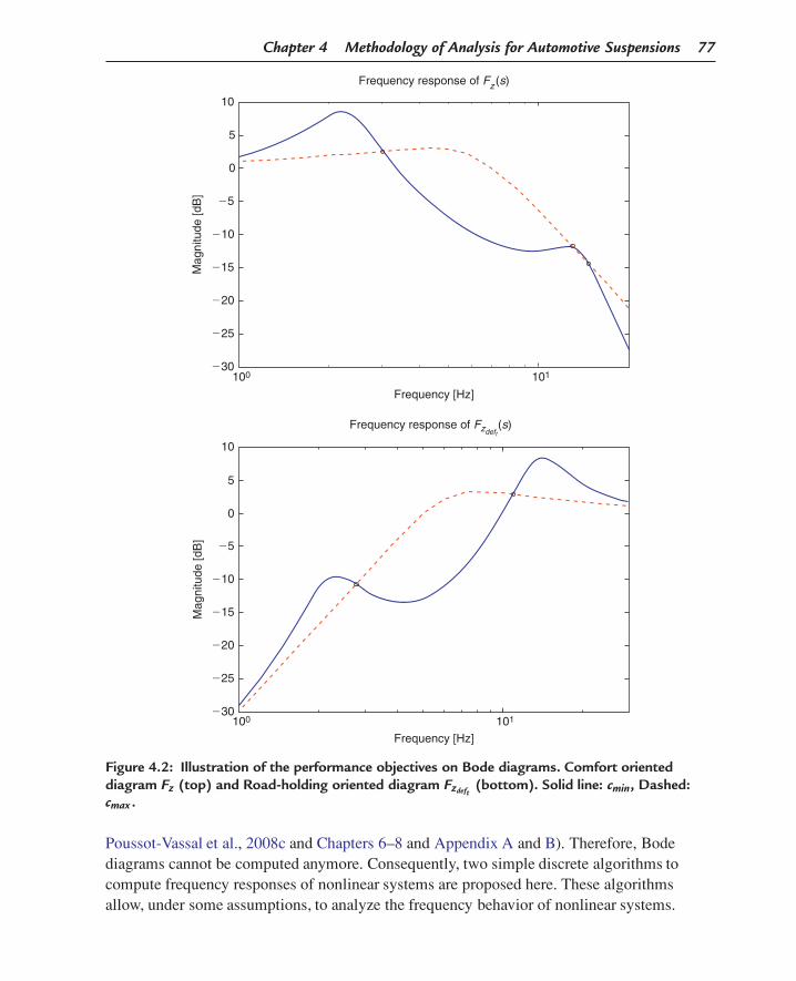
Figure 4.2 recalls the frequency responses of both main transfer functions under discussion inthis book, namely, Fz and Fzdeft

. Then let us define the comfort and road-holding performancesas follows.

4.1.4.1 Comfort

The vibration isolation between [0;20]Hz is evaluated by the transfer function Fz(s). Ideally,the vertical displacement of the chassis should be the same as the one of the road for lowfrequencies (lower than around 1 Hz) and attenuated for high frequencies (higher than 1 Hz),in order to filter undesirable vibrations. In practice, for low disturbances (zr < 3 cm), the


maximal gain occurring between 1 and 5 Hz of Fz(s) has to be lower than 1.8, and over thisfrequency, road disturbances should be filtered (see Sammier, 2001).

4.1.4.2 Road-Holding

As indicated before, it is evaluated using the transfer function Fzdeft(s) over the frequency

range of [0;30]Hz. For a good road-holding, the tire deflection should be attenuated for lowfrequencies, and filtered around the resonance frequency of the wheel and over. Moreover,especially for high frequencies, the wheel should always remain linked (i.e. in contact) tothe road.

Note that these objectives are consistent with the ones given in previous suspension analysisworks of Gillespie (1992) and Sammier et al. (2003). On Figure 4.2, the comfort androad-holding performances objectives are illustrated, considering the passive quarter-carmodel using the motorcycle parameters given in Table 1.2.

4.1.4.3 Deflection

The deflection signal should remain in the linear zone of the suspension system to avoid theend-stop zone (leading to discontinuities). This consideration is very important especiallywhen the comfort objective is to be reached.

Note that in this study, frequency limits will be fixed to 30 Hz. This choice is justified by thefact that, practically, higher frequencies are filtered by the vehicle mechanical elements.Therefore, it is not of great importance to extend the analysis over that frequency. Moreover,according to the quarter-car definition given in Chapter 3, this frequency limit is enough todescribe all the interesting behaviors (i.e. the two masses resonance peaks, the static gain, theattenuation area, etc.).

4.2 Frequency Domain Performance Evaluations

In the previous section, comfort and road-holding specifications were presented on aquarter-car vehicle, using “classical words”. This section is concerned with the description oftwo fundamental tools used throughout the book, namely: the frequency response (FR) andthe performance indexes. Let us now introduce the frequency domain based metrics used tomathematically characterize the suspension.

4.2.1 Nonlinear Frequency Response Computation

In order to evaluate the semi-active suspension performances, the frequency response (FR) ofthe system is evaluated. Since suspension models and/or controlled control algorithms may benonlinear, the closed-loop often turns to be nonlinear itself (see e.g. Aubouet et al., 2009;


100 101�30

�25

�20

�15

�10

�5

0

5

10

Mag

nitu

de [d

B]

Frequency response of Fz (s)

Frequency [Hz]

101

Frequency [Hz]100

�30

�25

�20

�15

�10

�5

0

5

10

Mag

nitu

de [d

B]

Frequency response of Fzdeft(s)

Figure 4.2: Illustration of the performance objectives on Bode diagrams. Comfort orienteddiagram Fz (top) and Road-holding oriented diagram Fzdeft

(bottom). Solid line: cmin, Dashed:cmax .

Poussot-Vassal et al., 2008c and Chapters 6–8 and Appendix A and B). Therefore, Bodediagrams cannot be computed anymore. Consequently, two simple discrete algorithms tocompute frequency responses of nonlinear systems are proposed here. These algorithmsallow, under some assumptions, to analyze the frequency behavior of nonlinear systems.


In the first one (Algorithm 1), the frequency response is evaluated frequency by frequencywhile the second one (Algorithm 2) excites multiple frequencies at the same time. For a linearsystem description, these two algorithms provide identical results, while for nonlinear systems,they may present some differences (but still provide similar results if signals are persistentenough). Note that the frequency representation is widely developed and used in both academicand industrial research since it provides a rich information set of the suspension performances.

According to Algorithm 1, the following comments should be kept into consideration:

• Applying this procedure to a linear system provides the so-called Bode diagram.• The P parameter aims at avoiding gain computation on transient behaviors of the nonlinear

system. By fixing P = 10 one computes the gain in the sinusoidal “steady state” behavior.• The interest in this FR computation (which is not representative of a real road profile

disturbance) is that it allows us to derive a Bode like diagram for nonlinear systems. In thisbook, this procedure is largely used to plot the frequency behavior of a suspension systemcontrolled (or not) through a nonlinear control law.

• Since the FR algorithm aims at characterizing the frequency response of nonlinearsystems, it is also important to note that the amplitude of the sinusoid disturbance willmodify the frequency response. Consequently, nonlinear analysis should also be carried

Algorithm 1 Nonlinear Frequency Response Computation F̃ – FR (Single Frequency)

To compute the approximate frequency response of F̃z( f ) – comfort characteristic – andF̃deft ( f ) – road-holding characteristic – of a (controlled) nonlinear suspension system, thefollowing procedure is applied:

1. A sinusoidal road disturbance zr (t) feeds the input of the nonlinear quarter vehicle models,over P periods such that:

zr (t) = A sin(2π ft) (4.6)

where A ∈ [1;5]cm, f ∈ [ f ; f ] ⊆ [1;30]Hz and t ∈ [P/ f ; P/ f ]s, where {P ∈ Z|P > 1}is the number of periods of the sinusoid feeding the system. Practically one may chooseP = 10.

2. The output signals y(t) are measured. Here, y(t) = z(t) (vertical suspended mass bounce)or z̈(t), and zde ft (t) = zt (t)− zr (t) (tire deflection).

3. For each signal the corresponding spectrum Y ( f ) of y(t) (and U( f ) of zr (t)) is computed(by means of a discrete Fourier Transform).

4. The power spectral density of Y ( f ) and U( f ) signals are computed; denoted as G y( f ) andGu( f ).

5. For each output signal of interest, the variance gain is computed as: F̃( f ) = G y( f )/Gu( f ).In our case, F̃z( f ) and F̃zde ft

( f ) signals are obtained.


through varying amplitudes. For the sake of readability, in this book, the disturbanceamplitude will often be reduced to one single amplitude where the suspension stays inits linear working point (i.e. A = 1 cm in Algorithm 1). Remember that on a realsuspension, nonlinearities will modify the dynamics (e.g. hysteresis phenomena, whichare often present in magnetorheological dampers, see Chapter 2).

Similarly to Algorithm 1, another approach can be used to derive the frequency response of anonlinear system. This approach consists in exciting the system at multiple frequencies atthe same time.

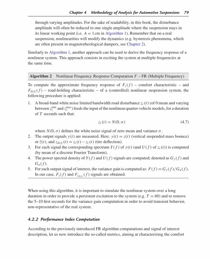
Algorithm 2 Nonlinear Frequency Response Computation F – FR (Multiple Frequency)

To compute the approximate frequency response of Fz( f ) – comfort characteristic – andFde ft( f ) – road-holding characteristic – of a (controlled) nonlinear suspension system, thefollowing procedure is applied:

1. A broad-band white noise limited bandwidth road disturbance zr (t) (of 0 mean and varyingbetween zmin

r and zmaxr ) feeds the input of the nonlinear quarter-vehicle models, for a duration

of T seconds such that:

zr (t) = N(0,σ ) (4.7)

where N(0,σ ) defines the white noise signal of zero mean and variance σ .2. The output signals y(t) are measured. Here, y(t) = z(t) (vertical suspended mass bounce)

or z̈(t), and zde ft (t) = zt (t)− zr (t) (tire deflection).3. For each signal the corresponding spectrum Y ( f ) of y(t) (and U( f ) of zr (t)) is computed

(by mean of a discrete Fourier Transform).4. The power spectral density of Y ( f ) and U( f ) signals are computed; denoted as G y( f ) and

Gu( f ).5. For each output signal of interest, the variance gain is computed as: F( f ) = G y( f )/Gu( f ).

In our case, Fz( f ) and Fzde ft( f ) signals are obtained.

When using this algorithm, it is important to simulate the nonlinear system over a longduration in order to provide a persistent excitation to the system (e.g. T = 60) and to removethe 5–10 first seconds for the variance gain computation in order to avoid transient behavior,non-representative of the real system.

4.2.2 Performance Index Computation

According to the previously introduced FR algorithm computations and signal of interestdescription, let us now introduce the so-called metrics, aiming at characterizing the comfort


and road-holding performances. These suspension performance measures (or indexes) aredefined as follows (note that two definitions are given, associated to each FR algorithm).

Definition 4.1 (Suspension performance measure J̃ -index). Let us define the functionC : R×R×R→ R, as follows:

C (X, f , f ) =∫ f

f|X ( f )|2d f (4.8)

where X ( f ) represents the frequency dependent signal of interest, obtained with Algorithm 1,f and f are the lower and upper bounds of the frequencies of interest. Then, the comfort androad-holding criteria are respectively defined as:

• J̃z̈, Comfort criterion (or J̃c):

J̃z̈ = C (F̃z̈,0,20)

C (F̃nomz̈ ,0,20)

(4.9)

• J̃zde ft, Road-holding criterion (or J̃rh):

J̃zde ft= C (F̃zde ft

,0,30)

C (F̃nomzde ft

,0,30)(4.10)

where F̃z̈ and F̃zde ftare the variance gains of the considered system obtained using

Algorithm 1. Then F̃nomz̈ and F̃nom

zde ftare the nominal suspension variance gains, i.e. the passive

uncontrolled reference suspension gains obtained by Algorithm 1 also.

Definition 4.2 (Suspension performance measure J -index). Let us define the functionC : R×R×R→ R, as follows:

C (X, t, t) =∫ t

t|x(t)|2dt (4.11)

where x(t) represents the time dependent signal of interest, obtained with the broad bandwhite noise signal used in the Algorithm 2, t and t represent the interval limits ofinterest. Then, the comfort and road-holding criteria are respectively defined as:

• Jz̈, Comfort criterion (or Jc):

Jz̈ = C (z̈, t , t)

C (z̈nom , t, t)(4.12)


• Jzde ft, Road-holding criterion (or Jrh):

Jzde ft= C (zde ft, t, t )

C (znomde ft

, t, t )(4.13)

where z̈ and zdeft are the time domain response signals obtained using Algorithm 2. Then z̈ nom

and znomdeft

are the time domain response signals of the passive uncontrolled referencesuspension gains obtained by Algorithm 2 also.

Remark 4.1 (Performance index interpretation). Performance measures given inDefinition 4.1 are ratios between the analyzed suspension and the reference suspensionconfiguration (which in our case will always be represented by a passive suspension witha nominal damping of c = 1500 Ns/m). Consequently, an improvement is obtained if theperformance measure is below 1. Therefore, if:

• Jz̈ > 1 or J̃z̈ > 1 (resp. Jz̈ < 1 or J̃z̈ < 1), it means that the analyzed suspension is less(resp. more) comfortable than the reference one.

• Jzde ft> 1 or J̃zde ft

> 1 (resp. Jzde ft< 1 or J̃zde ft

< 1), it means that the analyzed suspensionprovides worse (resp. better) road-holding performances than the reference one.

4.2.3 Numerical Discussion and Analysis

To illustrate the previously presented frequency domain response computation and theperformance index consistency, these metrics are now applied on a numerical example. Letus consider the passive quarter-car model, as in Definition 3.1 with the front motorcycleparameters given in Table 1.2. Then, the following damping values are evaluated:

• Nominal damping value, c = cnom = 1500 Ns/m, which is an average value, representing anice trade-off between comfort and road-holding performances.

• Soft damping value, c = cmin = 900 Ns/m, which is a low damping value, intuitivelyproviding more comfort oriented behavior (indeed, we will see that it is not completelytrue).

• Stiff damping value, c = cmax = 4300 Ns/m, which is a high damping value, intuitivelyproviding more road-holding oriented performances (indeed, we will see here again that itis not completely true).

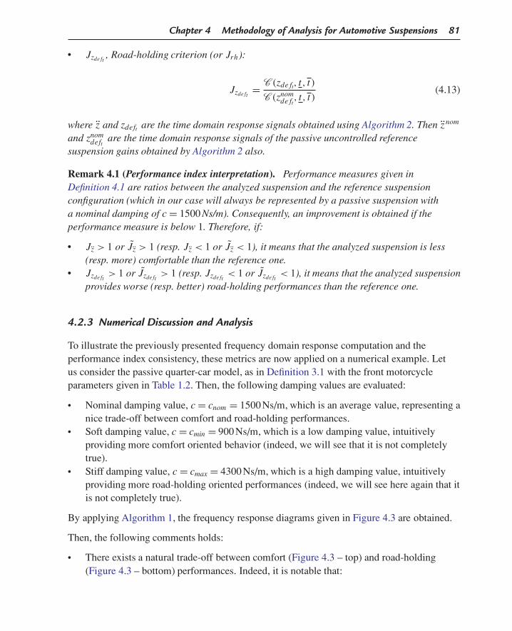
By applying Algorithm 1, the frequency response diagrams given in Figure 4.3 are obtained.

Then, the following comments holds:

• There exists a natural trade-off between comfort (Figure 4.3 – top) and road-holding(Figure 4.3 – bottom) performances. Indeed, it is notable that:


100�30

�25

�20

�15

�10

�5

0

5

10

Frequency [Hz]

Mag

nitu

de [d

B]

Frequency response of Fz

Passive (cnom)

Passive (cmin)

Passive (cmax)

�30

�25

�20

�15

�10

�5

0

5

10

Frequency [Hz]

Mag

nitu

de [d

B]

Frequency response of Fzdeft

101

100 101

Passive (cnom)

Passive (cmin)

Passive (cmax)

Figure 4.3: Nonlinear frequency responses (FR, obtained from Algorithm 1) of the passivequarter-car model for varying damping values: nominal c = 1500 Ns/m (solid line), softc = cmin = 900 Ns/m (dashed line) and stiff c = cmax = 4300 Ns/m (solid rounded line).Comfort oriented diagram F̃z (top) and Road-holding oriented diagram F̃zdef t

(bottom).


– No passive suspension configuration can provide both comfort (Fz) and road-holding(Fzde ft

) optimal characteristics.1

– No passive suspension configuration can globally improve filtering for either comfort(Fz) or road-holding (Fzde ft

) characteristics.• More specifically, the frequency space may roughly be divided in three zones:

– Low frequencies (in this case f ∈ [0;2]Hz), where the best filtering is achieved by thestiff damping configuration (c = cmax).

– Middle frequencies (in this case f ∈ [2;10]Hz), where the best filtering is achieved bythe soft damping configuration (c = cmin).

– High frequencies (in this case f ∈ [10;∞]Hz), where the best filtering is achieved by:* The stiff damping configuration (c = cmax), for road-holding objectives (bottom

frame).* The soft damping configuration (c = cmin), for comfort objectives (upper frame).

Let us note that, as illustrated in Chapter 5, this frequency space division is not so clear.

From that first frequency analysis, it appears that an optimal control should be able to adjustthe damping coefficient according to the road disturbance excitation (see Chapter 5 for moredetails). This analysis, justifies at a relatively high level, the use of a controlled damper toenhance the vehicle performances. From this analysis, it also appears that there is always atrade-off between comfort and road-holding performances. This trade-off simply means that apassive suspension cannot achieve both comfort and road-holding performances at the sametime, but, a controlled one should globally be better for both objectives. In Chapter 5, we willsee that controlled dampers cannot achieve optimal comfort and road-holding performances atthe same time.

Performance index is now investigated for the three damping configurations simulated onFigure 4.3 (i.e. either c = cnom = 1500 Ns/m, c = cmin = 900 Ns/m and c = cmax = 4300 Ns/m).Results are plotted on Figure 4.4.

According to the criteria in Definition 4.1, the suspension with nominal damping is selected asthe reference (nominal case). In Figure 4.4, both J̃c and J̃rh indexes of the passive nominaldamper are equal to 1. Then, according to the results of Figure 4.4, the following remarkshold:

• For a stiff suspension (c = cmax), the comfort criterion ( J̃c) is higher than one, hence thecar is uncomfortable (at least, less than the reference model), while the road-holdingcriterion ( J̃rh) is sightly lower than one, and hence provides better road-holding propertiesthan the passive one.

1 By optimal, one means, a better filtering i.e. a lower bound of the frequency response over all frequencies ofinterest; see Chapter 5 for more details.


0.5 1 1.5 2 2.50

0.2

0.4

0.6

0.8

1

1.2

1.4

1.6

1.8

2Normalized criteria: Comfort (left) Road-holding (right)

Passive (cnom)

Passive (cmin)

Passive (cmax)

Figure 4.4: Normalized performance criteria comparison for different damping values. Comfortcriterion – J̃c (left histogram set) and road-holding criterion – J̃rh (right histogram set).

• Conversely, when a soft suspension (c = cmin) is considered, the comfort criterion ( J̃c)

is lower than one, hence the car is comfortable, while the road-holding criterion ( J̃rh)

is higher than one, and hence provides worse road-holding performances than thepassive one.

Based on the same idea, these criteria can be evaluated for a large number of frozen dampingvalues c, leading to another interesting way to represent the trade-off between comfort androad-holding. On Figure 4.5, the performance indexes J̃c and J̃rh are evaluated for varyingdamping values (here c = [100, 10,000]). This figure illustrates the performance trade-offcurve of the passive suspension system. Each point of the curve gives the passive quarter-carmodel performance associated to a damping value; more specifically:

• the abscissa gives the comfort index ( J̃c);• the ordinate gives the road-holding index ( J̃rh);• while the line intensity changes as a function of the damping value c, (the darker, the

lower the damping is).

As defined, the point of coordinate (1;1) represents the passive nominal case. Then, bothpassive soft (c = cmin) and stiff (c = cmax) corresponding points are plotted on Figure 4.5.The interesting point to notice on this curve is that, as previously indicated by the frequencyresponses, the increase of the damping coefficient (i.e. c → ∞) will not improve the


Low damping

Comfort/Road-holding trade-off

Nominal damping

High damping

Roa

d-ho

ldin

g

1.4

1.3

1.2

1.1

1

0.80.8

0.9

Comfort

0.9 1 1.1 1.2 1.3 1.4 1.5 1.6 1.7

Figure 4.5: Normalized performance criteria trade-off ({ J̃c , J̃rh}) for a passive suspension system,with varying damping value c ∈ [100, 10 000] (solid line with varying intensity). Dots indicate thecriteria values for three frozen damping values (i.e. c = cmin = 900 Ns/m, c = cnom = 1500 Ns/mand c = cmax = 4300 Ns/m).

road-holding ( J̃rh), and conversely, the reduction of the damping value (i.e. c → 0) will notlead to a more comfortable vehicle ( J̃c). Therefore there exists an inherent trade-off foruncontrolled suspension. As we will see in Chapter 5, this trade-off is always true, even whendamper is perfectly controlled.

Remark 4.2 (About the trade-off curve). In the following chapters, this representation willbe re-used to:

• evaluate the best performances a controlled semi-active suspension system can achieve(Chapter 5);

• evaluate how semi-active strategies can improve passive suspension.

4.3 Other Time Domain Performance Evaluations

Up to now, only frequency domain analysis has been presented, in order to evaluate theglobal improvement. Here, time domain experiments are provided. The objective of thesetime domain experiments is to extend the frequency domain results, by evaluating the


0.4 0.45 0.5 0.55 0.6 0.650

0.01

0.02

0.03

0.04

0.05

0.06

t [s]

z r[m

]

Road disturbance profile (zr (t ))

100 101 102 103�220

�200

�180

�160

�140

�120

�100

�80

Frequency [Hz]

Gai

n [d

B]

Road disturbance spectrum (zr (f ))

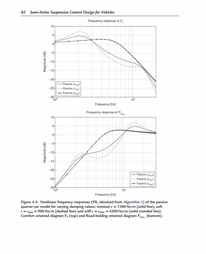
Figure 4.6: Bump road disturbance (top) and its time and frequency representation (bottom leftand right respectively).

suspension system subject to realistic road disturbances. The interest of these experiments isthat they are more easily understandable, and that they excite many frequencies at the sametime, while previous frequency tests excite one single frequency each time.

4.3.1 Bump Test

The bump test refers to a bump on the road which might be viewed as a high frequencyexcitation. The interest of this time domain experiment is that it is very likely to realize inpractice and to interpret. However, this test is only a complement to the previous ones, sinceit cannot represent all the suspension behaviors. Figure 4.6 illustrates a typical bump testprofile and its associated spectrum.

In the following, the previous test bench bump experiment is evaluated on the passivequarter-car model using motorcycle parameters. The experiments are done for two dampingconfigurations:


• Soft damping: c = cmin.• Stiff damping: c = cmax.

According to results given on Figure 4.7, the same comments as on the previous frequencyresults can be made. Basically, soft damping values provide lower accelerations and anoscillatory behavior, while stiff ones provide high accelerations and less oscillations. This

0 0.2 0.4 0.6 0.8 1 1.2 1.4 1.6 1.8 2�0.02

�0.01

0

0.01

0.02

0.03

0.04

0.05

0.06

z [m

]

�0.03

�0.02

�0.01

0

0.01

0.02

0.03

0.04

0.05

0 0.2 0.4 0.6 0.8 1 1.2 1.4 1.6 1.8 2

z def

�z t

�z r

[m]

Passive (cmin)

Passive (cmax)

Passive (cmin)

Passive (cmax)

t [s]

Chassis displacement

Tire deflection

t [s]

Figure 4.7: (Continued)


Passive (cmin)

Passive (cmax)

0 0.2 0.4 0.6 0.8 1 1.2 1.4 1.6 1.8 2�0.06

�0.04

�0.02

0

0.02

0.04

0.06

t [s]

Suspension deflection

z def

�z t

�z r

[m]

Figure 4.7: Road bump simulation of the passive quarter-car model for two configurations: harddamping (cmax, solid lines) and soft damping (cmin, dashed lines). Chassis displacement (z(t)),tire deflection (zdeft (t)) and suspension deflection (zdef (t)).

experiment is only given for practical issues, but will not give additional informationcompared to the frequency response.

4.3.2 Broad Band White Noise Test

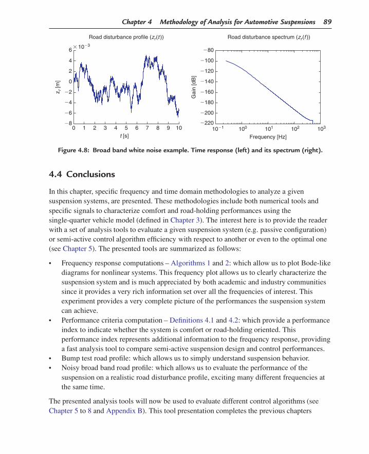
The white noise disturbance analysis consists in exciting the quarter-car model with a randomroad profile with limited bandwidth and amplitude, and analyzing the resulting performances.Since it represents a more realistic driving situation, this test is very interesting from theapplication point of view. The broad band white noise test is given on Figure 4.8. On the leftfigure, the broad band white noise is given in the time domain, while its associated spectrum isgiven on the right frame.

The frequency frame shows that the considered signal is attenuated as the frequency increases.Indeed this signal is generated as follows:

• Generate a random signal with zero mean value and a variance of 10 cm.• Apply an integral filter to this signal.

Since this signal is rich in frequency, the broad band white noise test is very interesting.However, it may be regarded as repetitive and hard to read compared to the frequencyresponse (FR) which gathers most of the important information a control engineer isinterested in. As a matter of fact, in this book, this experiment will not always be performed.


0 1 2 3 4 5 6 7 8 9 10�8

�6

�4

�2

0

2

4

6 � 10�3

t [s]

z r [m

]

Road disturbance profile (zr(t ))

10�1 100 101 102 103�220

�200

�180

�160

�140

�120

�100

�80

Frequency [Hz]

Gai

n [d

B]

Road disturbance spectrum (zr(f ))

Figure 4.8: Broad band white noise example. Time response (left) and its spectrum (right).

4.4 Conclusions

In this chapter, specific frequency and time domain methodologies to analyze a givensuspension systems, are presented. These methodologies include both numerical tools andspecific signals to characterize comfort and road-holding performances using thesingle-quarter vehicle model (defined in Chapter 3). The interest here is to provide the readerwith a set of analysis tools to evaluate a given suspension system (e.g. passive configuration)or semi-active control algorithm efficiency with respect to another or even to the optimal one(see Chapter 5). The presented tools are summarized as follows:

• Frequency response computations – Algorithms 1 and 2: which allow us to plot Bode-likediagrams for nonlinear systems. This frequency plot allows us to clearly characterize thesuspension system and is much appreciated by both academic and industry communitiessince it provides a very rich information set over all the frequencies of interest. Thisexperiment provides a very complete picture of the performances the suspension systemcan achieve.

• Performance criteria computation – Definitions 4.1 and 4.2: which provide a performanceindex to indicate whether the system is comfort or road-holding oriented. Thisperformance index represents additional information to the frequency response, providinga fast analysis tool to compare semi-active suspension design and control performances.

• Bump test road profile: which allows us to simply understand suspension behavior.• Noisy broad band road profile: which allows us to evaluate the performance of the

suspension on a realistic road disturbance profile, exciting many different frequencies atthe same time.

The presented analysis tools will now be used to evaluate different control algorithms (seeChapter 5 to 8 and Appendix B). This tool presentation completes the previous chapters


contents (Chapters 2 and 3) where controlled damper and vehicle models were presented.From now on, the reader is ready to analyze the principal semi-active control approachesexisting in the literature (Chapter 6) and evaluate the new approaches presented in thefollowing chapters (Chapters 5, 7 and 8).

The reader may also refer to the very complete work by Hrovat (1997), where suspensionperformance and analysis are well described.

Chapter 4 - Methodology of Analysis for Automotive Suspensions

Documents

Transcript of Chapter 4 - Methodology of Analysis for Automotive Suspensions