DEVELOPMENT OF A CONTROL STRATEGY FOR ROAD …etd.lib.metu.edu.tr/upload/12610392/index.pdf ·...

DEVELOPMENT OF A CONTROL STRATEGY FOR ROAD VEHICLES WITH SEMI-ACTIVE SUSPENSIONS USING A FULL VEHICLE RIDE

MODEL

A THESIS SUBMITTED TO THE GRADUATE SCHOOL OF NATURAL AND APPLIED SCIENCES

OF MIDDLE EAST TECHNICAL UNIVERSITY

BY

ZEYNEP ERDOĞAN

IN PARTIAL FULFILLMENT OF THE REQUIREMENTS FOR

THE DEGREE OF MASTER OF SCIENCE IN

MECHANICAL ENGINEERING

FEBRUARY 2009

Approval of the thesis:

DEVELOPMENT OF A CONTROL STRATEGY FOR ROAD VEHICLES WITH SEMI-ACTIVE SUSPENSIONS USING A FULL

VEHICLE RIDE MODEL

submitted by ZEYNEP ERDOĞAN in partial fulfilment of the requirements for the degree of Master of Science in Mechanical Engineering Department, Middle East Technical University by, Prof.Dr.Canan Özgen Dean, Graduate School of Natural Applied Sciences Prof.Dr.Süha Oral Head of Department, Mechanical Engineering Prof.Dr.Y.Samim Ünlüsoy Supervisor, Mechanical Engineering Dept., METU Examining Committee Members: Prof. Dr. Mehmet Çalışkan Mechanical Engineering Dept., METU Prof. Dr. Y. Samim Ünlüsoy Mechanical Engineering Dept., METU Asst. Prof. Dr. Yiğit Yazıcıoğlu Mechanical Engineering Dept., METU Dr. Gökhan Özgen Mechanical Engineering Dept., METU Asst. Prof. Dr. Kutluk Bilge Arıkan Mechatronics Engineering Dept., Atılım University Date: 12.02.2009

iii

I hereby declare that all information in this document has been obtained and presented in accordance with academic rules and ethical conduct. I also declare that, as required by these rules and conduct, I have fully cited and referenced all material and results that are not original to this work.

Name, Last name: Zeynep, Erdoğan

Signature:

iv

ABSTRACT

DEVELOPMENT OF A CONTROL STRATEGY FOR ROAD VEHICLES WITH SEMI-ACTIVE SUSPENSIONS USING A FULL RIDE VEHICLE MODEL

Erdoğan, Zeynep

M.S., Department of Mechanical Engineering

Supervisor: Prof. Dr. Y. Samim Ünlüsoy

February 2009, 112 pages

The main motivation of this study is the design of a control strategy for semi-active

vehicle suspension systems to improve ride comfort for road vehicles. In order to

achieve this objective, firstly the damping characteristics of Magnetorheological

dampers will be reviewed. Then an appropriate semi-active control strategy

manipulating the inputs of the dampers to create suitable damping forces will be

designed. Linear Quadratic Regulator (LQR) control strategy is the primary focus

area on semi-active control throughout this study. Further, skyhook controllers are

examined and compared with optimal LQR controllers. The semi-active controller is

tuned using a linearized full (4 wheel) vehicle ride model with seven degrees of

freedom. Some selected simulations are carried out by using a nonlinear model to

tune LQR controller in an effort to optimize bounce, pitch, and roll motion of the

vehicle. Time domain simulations and frequency response analysis are used to justify

the effectiveness of the proposed LQR control strategy.

Keywords: Semi-active Suspensions, Magnetorheological Damper, Linear Quadratic

Regulator, Optimal Control, Optimization, Skyhook, Full Vehicle Ride Model

v

ÖZ

YARI AKTĐF SÜSPANSĐYONLAR ĐÇĐN TAM ARAÇ MODELĐ KULLANARAK KONTROL STRATEJĐLERĐNĐN GELĐŞTĐRĐLMESĐ

Erdoğan, Zeynep

Yüksek Lisans, Makine Mühendisliği Bölümü

Tez Yöneticisi: Prof. Dr. Y. Samim Ünlüsoy

Şubat 2009, 112 sayfa

Bu tez çalışmasının amacı, yarı-aktif süspansiyon sistemleri için kullanılan kontrol

stratejilerinin yol araçlarının sürüş komforunu geliştirmek için tasarlanmasıdır. Bu

çalışmada öncelikle manyetoreolojik sönümleyiciler araştırılmış, daha sonra araç

modelinde süspansiyonların uygulaması gereken sönümleme kuvvetlerinin

belirlenebilmesi için yarı-aktif kontrol stratejisi geliştirilmiştir. Lineer Karesel

Durum Regülatörü (LKR) bu çalışmada öncelikle kullanılan yarı-aktif kontrol

stratejisidir. Buna ek olarak “Skyhook” kontrolcüsü incelenmiş ve LKR

kontrolcüsüyle performans açısından karşılaştırılmıştır. Yarı-aktif kontrol stratejisi

doğrusal yedi serbestlik dereceli (4 tekerlekli) araç modeli kullanılarak ayarlanmış;

seçilen bazı simülasyonlarla, doğrusal olmayan modelde sistemin zıplama, başvurma

ve yalpalama davranışları eniyilenmiştir. Zamana bağlı simülasyonlarla ve frekans

cevabı analizleriyle LKR denetleyicisinin yeterliliği gösterilmiştir.

Anahtar Kelimeler: Yarı aktif Süspansiyon, Manyetoreolojik Sönümleyici, Lineer

Karesel durum Regülatörü, Eniyi Denetim, Eniyileme, “Skyhook”, Tam Araç Sürüş

Konforu Modeli

vi

ACKNOWLEDGEMENTS

First, I would like to express my special thanks to my supervisor Prof. Dr. Y. Samim

Ünlüsoy, who has guided me to this topic with his experience, endlessly supported

and encouraged me. Additionally I want to thank Prof. Dr. Bülent Platin for opening

his doors when I needed help. I would also like to state my gratitude to my colleague

Kemal Çalışkan for his assistance in developing user interfaces in Matlab. Also,

financial support of TÜBĐTAK is also gratefully acknowledged.

It would not be easy for me to write my master degree thesis without the help and

support of my friends Tuğçe Yüksel, Ali Murat Kayıran, Zekai Murat Kılıç and

Bekir Bediz.

I would like to express my special thanks to Gökhan Tekin who has supported and

cheered me up in all my hard times and gave me the strength to carry on.

Finally I would also like to thank my precious parents Şükran and Esat Erdoğan for

their unconditional continuous support throughout my life. The last but not the least,

I would like to thank my sister Bilge Erdoğan for making me feel she is always

standing by my side despite the long distances between us.

vii

TABLE OF CONTENTS

ABSTRACT ................................................................................................................ iv

ÖZ ................................................................................................................................ v

ACKNOWLEDGEMENTS ....................................................................................... vi

TABLE OF CONTENTS ........................................................................................... vii

LIST OF FIGURES ..................................................................................................... x

LIST OF TABLES .................................................................................................... xiv

LIST OF SYMBOLS ................................................................................................. xv

LIST OF ABBREVIATIONS .................................................................................. xvii

1 INTRODUCTION ............................................................................................... 1

1.1 RESEARCH OBJECTIVES ................................................................................... 1

1.2 APPROACH ........................................................................................................... 2

1.3 BACKGROUND .................................................................................................... 2

1.3.1 MAGNETORHEOLOGICAL FLUID TECHNOLOGY .......................................... 3

1.4 LITERATURE SURVEY....................................................................................... 8

1.5 OUTLINE ............................................................................................................. 13

2 FULL-CAR VEHICLE RIDE MODEL ............................................................ 15

2.1 INTRODUCTION ................................................................................................ 15

2.2 EQUATIONS OF MOTION OF THE FULL-CAR RIDE MODEL ................... 16

2.2.1 NONLINEAR EQUATIONS WITH PASSIVE SUSPENSIONS .......................... 16

2.2.2 STATE SPACE REPRESENTATION OF THE LINEAR PASSIVE SYSTEM .... 18

2.2.3 EQUATIONS OF MOTION IN STATE SPACE FORM ....................................... 20

2.2.4 STATE SPACE REPRESENTATION OF THE LINEAR SEMI-ACTIVE

SYSTEM ................................................................................................................................ 24

3 SEMI-ACTIVE CONTROL STRATEGY ........................................................ 29

viii

3.1 INTRODUCTION ................................................................................................ 29

3.2 SENSOR REQUIREMENTS ............................................................................... 30

3.3 MR MODELLING ............................................................................................... 31

3.4 OPTIMAL CONTROL/ LINEAR QUADRATIC REGULATOR CONTROL

STRATEGY ...................................................................................................................... 31

3.4.1 A THEORETICAL LOOK INTO LINEAR QUADRATIC REGULATOR

CONTROL STRATEGY............................................................................................................ 32

3.4.2 THE LIMITATIONS OF TIME-INVARIANT LINEAR QUADRATIC

REGULATOR ............................................................................................................................ 33

3.4.3 FEASIBILITY OF LQR CONTROL INPUTS FOR SEMI-ACTIVE DAMPERS. 34

3.5 SKYHOOK, GROUNDHOOK CONTROL STRATEGY .................................. 39

4 SIMULATION MODEL .................................................................................... 41

4.1 SIMULINK MODEL ........................................................................................... 41

4.2 OPTIMAL CONTROLLER BLOCKS ................................................................ 41

4.3 SKYHOOK CONTROLLER BLOCKS .............................................................. 44

5 OPTIMIZATION PROCESS ............................................................................. 45

5.1 THEORETICAL BACKGROUND ..................................................................... 45

5.1.1 TRANSMISSIBILITY ANALYSIS OF QUARTER CAR MODEL ...................... 45

5.1.2 VIBRATION ANALYSIS OF FULL CAR RIDE MODEL ................................... 51

5.2 OPTIMIZATION FOR OPTIMAL CONTROL USING BUMP INPUT ............ 52

5.2.1 STAGE 1: OPTIMIZATION WITH RESPECT TO ONLY BOUNCE

WEIGHTING FACTOR ............................................................................................................. 53

5.2.2 STAGE 2: OPTIMIZATION WITH RESPECT TO ONLY PITCH WEIGHTING

FACTOR ................................................................................................................................ 55

5.2.3 STAGE 3: OPTIMIZATION WITH RESPECT TO BOUNCE ACCELERATION

FACTOR AND PITCH WEIGHTING FACTOR ...................................................................... 58

5.2.4 STAGE 4: OPTIMIZATION WITH RESPECT TO BOUNCE ACCELERATION,

PITCH AND ROLL WEIGHTING FACTOR ........................................................................... 64

5.3 3D BUMP OPTIMIZATION FOR SKYHOOK CONTROL STRATEGIES ..... 68

5.4 3D CHIRP INPUT ANALYSIS ........................................................................... 69

6 SIMULATION TESTS ...................................................................................... 75

6.1 SINUOSIDAL INPUT TEST ............................................................................... 75

6.2 BUMP&HUMP TEST .......................................................................................... 78

6.2.1 HALF SINUSOIDAL BUMP TEST SIMULATION 1 .......................................... 78

ix

6.2.2 HALF SINUSOIDAL BUMP TEST SIMULATION 2 .......................................... 82

6.2.3 HALF SINUSOIDAL HUMP TEST ....................................................................... 85

6.3 STEP INPUT TEST ............................................................................................. 87

6.4 RANDOM ROAD INPUT TEST ......................................................................... 90

7 CONCLUSION .................................................................................................. 95

REFERENCES ........................................................................................................... 97

APPENDICES

APPENDIX A .......................................................................................................... 101

A.1 GENERAL VIEW OF THE SIMULATION MODEL SIMULATION MODEL

………………………………………………………………………………… 101

A.2 ROLL AND PITCH MOTION OF THE VEHICLE .......................................... 102

A.3 COMPABILITY EQUATIONS BETWEEN CENTRE OF MASS AND

CORNERS OF THE VEHICLE ...................................................................................... 103

A.4 UNSPRUNG MASS MOTION .......................................................................... 104

A.5 BOUNCE MOTION OF THE VEHICLE .......................................................... 105

APPENDIX B .......................................................................................................... 106

APPENDIX C .......................................................................................................... 107

APPENDIX D .......................................................................................................... 110

APPENDIX E .......................................................................................................... 112

x

LIST OF FIGURES

FIGURES

Figure 1.1 Illustrative Sketch ....................................................................................... 5

Figure 1.2 The Characteristics of CARRERATM MagneShockTM Damper ................. 6

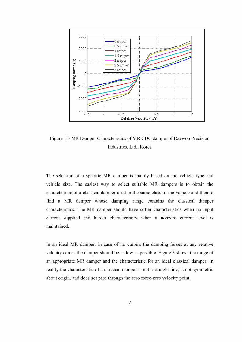
Figure 1.3 MR Damper Characteristics of MR CDC damper of Daewoo Precision

Industries, Ltd., Korea .................................................................................................. 7

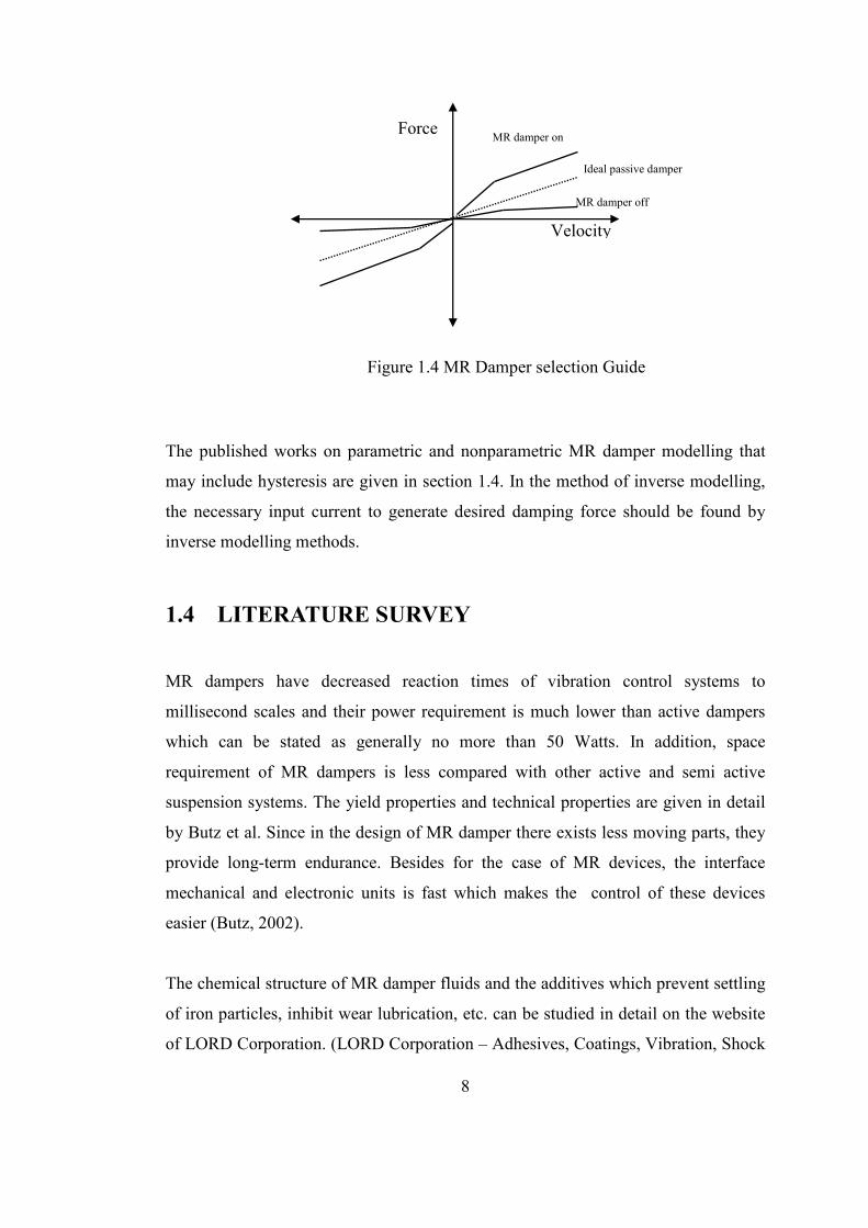
Figure 1.4 MR Damper selection Guide ...................................................................... 8

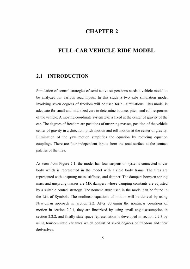
Figure 2.1 Full Car Ride Model ................................................................................. 16

Figure 3.1 Semi-Active Damper Control Concept ..................................................... 30

Figure 3.2 Admissible Damping Region of a Typical Semi-Active Damper ............ 34

Figure 3.3 Process of Clipping Optimal Forces to Admissible Damping Region ..... 36

Figure 3.4 Quarter Car Model .................................................................................... 40

Figure 4.1 Full State Feedback Optimal Control Simulink Model ............................ 42

Figure 4.2 MR Modelling And Force Clipping Simulink Model .............................. 43

Figure 4.3 Skyhook Controller Simulink Model........................................................ 44

Figure 5.1 Quarter Car Model .................................................................................... 45

Figure 5.2 Transmissibility of Sprung Mass Acceleration with Respect to Road Input

.................................................................................................................................... 46

Figure 5.3 Transmissibility of Sprung Mass Displacement with Respect to Road

Input ........................................................................................................................... 46

Figure 5.4 Transmissibility of Rattle Space with respect to Road Input ................... 47

Figure 5.5 Transmissibility of Unsprung Mass Acceleration with respect to Road

Input ........................................................................................................................... 48

Figure 5.6 Transmissibility of Tire Deflection with respect to Road Input ............... 48

xi

Figure 5.7 Weighting Constants for Sinusoidal Bump Body Bounce Acceleration

Optimization ............................................................................................................... 54

Figure 5.8 Bump Simulation Results (RMS Body Bounce Acceleration) ................. 54

Figure 5.9 Sinusoidal Bump Simulation Results (Peak To Peak Body Bounce

Acceleration) .............................................................................................................. 55

Figure 5.10 Weighting Constants for Sinusoidal Bump Pitch Angle Optimization .. 56

Figure 5.11 Sinusoidal Bump Simulation Results (RMS of Pitch Angle) ................. 57

Figure 5.12 Sinusoidal Bump Simulation Results (Peak To Peak Pitch Angle) ........ 57

Figure 5.13 Sinusoidal Bump Simulation Results (RMS of Bounce Acceleration) .. 60


Figure 5.15 Sinusoidal Bump Simulation Results (RMS of Bounce Acceleration) .. 63


Figure 5.17 Sinusoidal Bump 3D Simulation Results (RMS of Bounce Acceleration)

.................................................................................................................................... 67

Figure 5.18 Sinusoidal Bump 3D Simulation Results (RMS of Pitch Angle) ........... 67

Figure 5.19 Sinusoidal Bump 3D Simulation Results (RMS of Roll Angle) ............ 68

Figure 5.20 Power Spectral Density of Bounce Displacement and Acceleration -

Chirp Input from 4 Wheels ........................................................................................ 71

Figure 5.21 Power Spectral Density of Bounce Acceleration - Chirp Input from one

Wheel ......................................................................................................................... 71

Figure 5.22 Power Spectral Density of Pitch Motion - Chirp Input from one Wheel 72

Figure 5.23 Power Spectral Density Of Roll Motion - Chirp Input From One Wheel

.................................................................................................................................... 73

Figure 5.24 Power Spectral Density of Rattle Space Motion - Chirp Input from One

Wheel ......................................................................................................................... 74

Figure 6.1 Bounce Displacement and Acceleration versus Time – Sinusoidal Input 76

Figure 6.2 Pitch Angle versus Time - Sinusoidal Input ............................................. 76

Figure 6.3 Roll Angle versus Time - Sinusoidal Input .............................................. 77

Figure 6.4 Rattle Space versus Time - Sinusoidal Input ............................................ 77

xii

Figure 6.5 Road Input versus Time - Half Sinusoidal Bump Input Case 1 ............... 79

Figure 6.6 Bounce Displacement and Bounce Acceleration versus Time - Half

Sinusoidal Bump Case 1 ............................................................................................ 80

Figure 6.7 Pitch Angle versus Time - Half Sinusoidal Bump Case 1 ........................ 80

Figure 6.8 Roll Angle versus Time - Half Sinusoidal Bump Input Case 1 ................ 81

Figure 6.9 Rattle Space Motion of Front Left Suspension and Rear Right Suspension

versus Time - Half Sinusoidal Bump Input Case 1 .................................................... 81

Figure 6.10 Road Input versus Time - Half Sinusoidal Bump Input Case 2 ............. 82

Figure 6.11 Bounce Motion And Bounce Acceleration versus - Half Sinusoidal

Bump Input Case 2 ..................................................................................................... 83

Figure 6.12 Pitch Motion versus Time - Half Sinusoidal Bump Input Case 2 .......... 83

Figure 6.13 Roll Motion versus Time - Half Sinusoidal Bump Input Case 2 ............ 84

Figure 6.14 Rattle Space Motion of Front Left Suspension and Rear Right

Suspension versus Time - Half Sinusoidal Bump Input Case 2................................. 84

Figure 6.15 Road Input versus Time - Half Sinusoidal Hump Input ......................... 85


Hump Input ................................................................................................................ 86

Figure 6.17 Pitch Motion versus Time - Half Sinusoidal Hump Input ...................... 86


Suspension versus Time - Half Sinusoidal Hump Input ............................................ 87

Figure 6.19 Step Road Input versus Time .................................................................. 88

Figure 6.20 Bounce Motion versus Time Step Input ................................................. 88

Figure 6.21 Pitch Motion versus Time Step Input ..................................................... 89


Suspension versus Time - Step Input ......................................................................... 89

Figure 6.23 Random Road Input versus Time ........................................................... 90

Figure 6.24 MR and Passive Damper Characteristics ................................................ 92

Figure 6.25 Power Spectral Density of Bounce Displacement and Bounce

Acceleration of the existing MR damper ................................................................... 92

xiii


Acceleration of the fictious MR damper .................................................................... 93

Figure A.1 General view of the Simulink Model ..................................................... 101

Figure A.2 Simulink Model for Roll and Pitch Motion ........................................... 102

Figure A.3 Simulink Model for Compatibility Equations ....................................... 103

Figure A.4 Simulink Model of Unsprung Mass Motion .......................................... 104

Figure A.5 Simulink Model for Bounce Motion ...................................................... 105

Figure E.1 MR Data used in Simulations ................................................................ 112

xiv

LIST OF TABLES

TABLES

Table 1 Natural Frequencies of Full Car Ride Model ................................................ 51

Table 2 Weighting Constants for 2D Optimization ................................................... 59

Table 3 Weighting Constants for 3D Bump Optimization......................................... 65

Table 4 Performance Results for the MR Damper under Random Road Input ......... 94

Table 5 Performance Results for the Fictitious MR Damper under Random Road

Input ........................................................................................................................... 94

Table 6 Vehicle Data Used in Vehicle Simulations ................................................. 106

xv

LIST OF SYMBOLS

n

2

φ = pitch angle

ρ=road roughness parameter

ρ =weighting factor

σ cov ariance

θ = roll angle

a = longitudinal distance from sprung mass center to front suspension

A= state matrix of the vehicle in state space

=

representation

b = longitudinal distance from sprung mass center to rear suspension

B= disturbance matrix in state space representation

c = lateral distance from sprung mass center to right suspension

C

bl1

bl2

br1

=input matrix in state space representation/damping matrix

c = damping constant of rear left tyre

c = rear left MR damping consant between sprung and unsprung masses

c = damping constant of

br2

fl1

fl2

rear right tyre

c = rear right MR damping consant between sprung and unsprung masses

c = damping constant of front left tyre

c = front left MR damping consant between sprung and unsprung mas

fr1

fr2

g

ses

c = damping constant of front right tyre

c = front right MR damping consant between sprung and unsprung masses

d = lateral distance from sprung mass center to right suspension

G =groundhook con

s

bl

br

fl

fr

stant

G =skyhook constant

K=closed loop gain matrix/stiffness matrix

m = rear left unsprung mass

m = rear right unsprung mass

m = front left unsprung mass

m = front right unsprung mass

M= sprung mass

1 2 3

of the car

P ,P ,P =performance indices

Q,R,N=design matrices for quadratic cost functions

S=solution of algebraic riccati equation

xvi

bl0

bl1

bl2

u=input

v=velocity

w=disturbance

W=white noise

x=states in the state space representation of the vehicle model

z = road input to rear left tyre

z = position of rear left unsprung mass

z = position of r

br0

br1

br2

cg

fl0

ear left sprung mass

z = road input to rear right tyre

z = position of rear right unsprung mass

z = position of rear right sprung mass

z = position of sprung mass

z = road input to front left tyre

fl1

fl2

fr0

fr1

fr2

z = position of front left unsprung mass

z = position of front left sprung mass

z =road input to front right tyre

z = position of front right unsprung mass

z = position of front right sprung mas

1

2

s

z = position of unsprung mass in a quarter car model

z = position of sprung mass in a quarter car model

all first derivatives will have upscript " " and second derivatives will have " "ɺ ɺɺ

xvii

LIST OF ABBREVIATIONS

ER Electrorheological

FAMOS Frequency Adaptive Multi-objective

H2 H2 control

H∞ H infinity control

HILS Hardware-in-the-Loop Simulations

IMU Inertial Measurement Unit

LDT Linear Displacement Transducer

LQG Linear Quadratic Gaussian

LQR Linear Quadratic Regulator

MIMO Multi Input Multi Output System

MR Magnetorheological

OGS Optimal Gain Switching Target

PID Proportional Integral Derivative

PSD Power Spectral Density

RMS Root Mean Square

SID Simplified Inverse Dynamics

SISO Single Input Single Output System

1

CHAPTER 1

1

1 INTRODUCTION

1.1 RESEARCH OBJECTIVES

In classical vehicle dynamics, there exists three main subjects of interest: vehicle

handling, ride comfort, and performance. The first subject is mainly concerned on

stability and controllability of the vehicle by the driver during cornering manoeuvres.

The second subject refers to the quality of the isolation of vehicle passengers from

outer disturbances such as road bumps and roughness, external inputs, etc. Without

any doubt, the design of appropriate suspension systems is the most crucial part for

obtaining ride comfort objectives which will inevitably affect vehicle handling.

There are three types of suspension systems namely passive, semi-active, and active

suspension systems. The latter suspension systems are developed to improve

conventional passive suspension characteristics. Semi-active and active dampers can

adjust their forces according to road conditions. Active suspension systems are

superior in improving handling and ride characteristics of a vehicle whereas passive

dampers have the advantage of the simplicity and low cost. A semi-active suspension

system using magnetorheological (MR) dampers is a compromise between active and

passive suspension systems. They have lower cost than active suspension systems

and while they are superior in improving ride comfort and road holding to passive

suspensions. More general information on suspension system types can be found in

section 2.1.

The main objective of this study is to build a design methodology for constructing a

controller system for the semi active vehicle suspension systems to improve ride

2

comfort. The methodology targets basic ride comfort through controlling the vehicle

suspension system. The suspension system is to be designed to obtain a compromise

between different ride comfort objectives such as sprung mass acceleration roll and

pitch motions of the vehicle. The designed controller system will be tested in order to

verify its performance.

1.2 APPROACH

The study on semi-active suspensions is carried with Magnetorheological(MR)

dampers which are discussed in detail in section 2.2. Clipped Linear Quadratic

Regulator (LQR) optimal control strategy is chosen as the main control strategy to

minimize bounce acceleration, and roll and pitch motions of the vehicle by

modifying the damper characteristics. The full ride model (seven degree of freedom)

with the proposed controller is tested for several road inputs and the controller is

tuned based on the simulation tests that will be discussed in chapter 4.

1.3 BACKGROUND

In conventional vehicles, the suspension system between sprung and unsprung

masses is usually composed of a spring and a conventional damper in parallel. The

parameters of the spring and damper are set to make a compromise between ride

comfort and handling. To get better handling and ride comfort characteristics

simultaneously, the use of active and semi-active suspension systems has become a

recent focus area in automotive industry.

Active systems can supply and dissipate energy to/from a system. There is a force

actuator that can provide necessary force to the system. The response of the system

can be adjusted according to road inputs. The main disadvantage is the high power

demand from the vehicle power sources.

3

Semi-active damper systems can provide the variation of damping coefficient of the

damper. They, however, can only dissipate energy from the system. Power

requirement of these systems is usually lower than active suspensions. Although

active suspensions has superiority in performance, semi-active suspensions are more

feasible for implementation in vehicles because of their cost advantage, low power

requirement and simplicity.

Some varieties of semi-active devices are controllable friction devices, variable

orifice dampers, electrorheological (ER) fluid dampers, and magnetorheological

(MR) fluid dampers. The friction coefficient can be regulated in controllable friction

dampers, more information on controllable friction devices can be taken from

(Guglielmino, 2008). The orifice openings consequently are regulated in variable

orifice dampers such that necessary damping forces are generated (Rajamani, 2006).

MR and ER semi-active dampers are fluid dampers which change their viscosity

according to the current supplied to the system.

MR dampers have become the search focus for semi-active dampers, since their

available damping range and the response time are almost as good as active dampers

in spite of the lower power requirement. The next section provides more detailed

information on MR fluids and MR dampers.

1.3.1 MAGNETORHEOLOGICAL FLUID TECHNOLOGY

In the 1940’s, MR fluid technology and its possible application areas have become

known in the scientific areas. However the availability of MR fluids was greatly

enhanced later on by the development of electronic technology such as controllers,

microprocessors and sensors. After 1980, MR fluids have started to be used in many

application areas (Grad, 2006). The application areas of the MR technology are quite

wide. These applications can be seen from (Klingenberg, 2001). MR technology can

be used in prosthetic knees, in civil engineering to reduce earthquake effects in

structures, polishing industry, gun recoil mechanisms, and washing machines. One of

4

the main application areas is in the automotive industry. Besides its obvious use in

shock absorbers; it can also be used in clutches, passenger seat suspensions, and

brakes. The paper by Klingenberg also addresses the possible challenges in MR

technology like decreasing cost, overcoming sedimentation, and oxidation of iron

particles.

MR dampers were used as primary suspensions on models of Acura MDX, Audi TT,

Audi R8, Buick Lucerne, Cadillac DTS, Cadillac SLR, Cadillac SRX, Cadillac STS,

Chevrolet Corvette, Ferrari 599GTB and Holden HSV Commodore (Primary

Suspension, 2008).

1.3.1.1 Magnetorheological Fluid Characteristics

Magnetorheological (MR) fluids are kind of a fluid with magnetic particles that

change rheological characteristics in response to application of a magnetic field.

Magnetic particles align and develop yield strength in the presence of a magnetic

field. The yield strength of the fluid can be modified by changing the magnetic field

strength. Usually the yield stress increases by the magnetic field applied. In the work

of Klingenberg (Klingenberg, 2001), it is stated that the flow behaviour of MR fluids

is typically like a Bingham fluid which does not flow unless the stress exerted is

above the yield strength of the fluid. In the absence of a magnetic field, the fluid

behaviour is like Newtonian fluids. It is also claimed that the MR fluids are not

sensitive to contaminants and unaffected by temperature and the changes in

rheological behaviour of the fluid take less than 10 milliseconds (Technology

Compared, n.d.).

1.3.1.2 MR Damper Characteristics

MR dampers have received attention in engineering environments because they offer

variable damping characteristics. They are mainly used as semi active automotive

suspension systems. Thus, semi active devices are expected to offer effective

performance over a variety of amplitude and frequency ranges. Although the active

5

dampers are superior in order to reach that goal, they have higher power

requirements than semi active dampers and they cost. Considering the performances

of suppressing vibration of the sprung and unsprung masses, they achieve significant

performance achievement when compared to conventional passive suspensions.

Figure 1.1 Illustrative Sketch

MR dampers have nonlinear damping characteristics with hysteresis. MR damper

characteristics depend on both input current and the relative velocity across

suspension ends. The hysteresis can be seen from the illustrative Figure 1.1 which is

inspired from the article of Butz et. al. (Butz, 2002). Figure 1.1 shows the damping

force changes due to relative velocity at a specified constant current value. In low

relative velocity region across the suspension, the damping behaviour is quite

unpredictable, however in high relative velocity regions; the damping characteristic

is quite linear. The models used in simulations generally do not include hysteresis in

order to simplify and linearize the system.

Generally as the input current becomes higher, the damping force available at a

particular relative velocity becomes higher. From Figure 1.2 which shows the

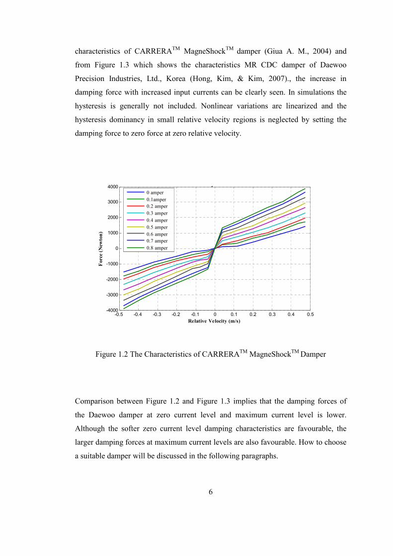
6

characteristics of CARRERATM MagneShockTM damper (Giua A. M., 2004) and

from Figure 1.3 which shows the characteristics MR CDC damper of Daewoo

Precision Industries, Ltd., Korea (Hong, Kim, & Kim, 2007)., the increase in

damping force with increased input currents can be clearly seen. In simulations the

hysteresis is generally not included. Nonlinear variations are linearized and the

hysteresis dominancy in small relative velocity regions is neglected by setting the

damping force to zero force at zero relative velocity.

Figure 1.2 The Characteristics of CARRERATM MagneShockTM Damper

Comparison between Figure 1.2 and Figure 1.3 implies that the damping forces of

the Daewoo damper at zero current level and maximum current level is lower.

Although the softer zero current level damping characteristics are favourable, the

larger damping forces at maximum current levels are also favourable. How to choose

a suitable damper will be discussed in the following paragraphs.

0

0.1

0.2

0.3

0.4

0.5

0.6

0.7

0.8

0.9

1

-0.5 -0.4 -0.3 -0.2 -0.1 0 0.1 0.2 0.3 0.4 0.5-4000

-3000

-2000

-1000

0

1000

2000

3000

4000

Relative Velocity (m/s)

For

ce (

New

ton

)

0 amper

0.1amper0.2 amper

0.3 amper

0.4 amper

0.5 amper

0.6 amper0.7 amper

0.8 amper

7

Figure 1.3 MR Damper Characteristics of MR CDC damper of Daewoo Precision

Industries, Ltd., Korea

The selection of a specific MR damper is mainly based on the vehicle type and

vehicle size. The easiest way to select suitable MR dampers is to obtain the

characteristic of a classical damper used in the same class of the vehicle and then to

find a MR damper whose damping range contains the classical damper

characteristics. The MR damper should have softer characteristics when no input

current supplied and harder characteristics when a nonzero current level is

maintained.

In an ideal MR damper, in case of no current the damping forces at any relative

velocity across the damper should be as low as possible. Figure 3 shows the range of

an appropriate MR damper and the characteristic for an ideal classical damper. In

reality the characteristic of a classical damper is not a straight line, is not symmetric

about origin, and does not pass through the zero force-zero velocity point.

8

The published works on parametric and nonparametric MR damper modelling that

may include hysteresis are given in section 1.4. In the method of inverse modelling,

the necessary input current to generate desired damping force should be found by

inverse modelling methods.

1.4 LITERATURE SURVEY

MR dampers have decreased reaction times of vibration control systems to

millisecond scales and their power requirement is much lower than active dampers

which can be stated as generally no more than 50 Watts. In addition, space

requirement of MR dampers is less compared with other active and semi active

suspension systems. The yield properties and technical properties are given in detail

by Butz et al. Since in the design of MR damper there exists less moving parts, they

provide long-term endurance. Besides for the case of MR devices, the interface

mechanical and electronic units is fast which makes the control of these devices

easier (Butz, 2002).

The chemical structure of MR damper fluids and the additives which prevent settling

of iron particles, inhibit wear lubrication, etc. can be studied in detail on the website

of LORD Corporation. (LORD Corporation – Adhesives, Coatings, Vibration, Shock

Force

Velocity

MR damper off

damping

MR damper on

Ideal passive damper

Figure 1.4 MR Damper selection Guide

9

& Motion Control., n.d.). LORD Corporation is one of the leading companies in MR

technology in corporation with Delphi's MagneRide™ shock absorbers, and

Carrera’s MagneShock™ automotive racing shocks absorbers. MR technology has

been adapted to Cadillac Seville STS and Chevrolet Corvette. Today the MagneRide

system is in production on the Cadillac SRX, SLR, and DTS and the new Buick

Lucerne. From the website of LORD Corporation (Primary Suspension, 2008),

introductory technical papers about the rheological, magnetic, and material properties

of various commercial MR fluids can be found. Also possible application areas can

be found in the article by Jolly et al.(Mark R. Jolly, 1999).

Modelling MR damper characteristics and behaviour estimation is generally done by

constructing look-up tables or estimated behaviour curves. Sung et al. (Sung K. C.,

2005) studied three modes of operation of MR dampers; namely flow (valve), shear

mode, and squeeze mode. The flow mode is more related to the thesis subject since

this mode is suitable for shock absorbers and dampers. The paper also discusses

other application areas of MR fluids and the problems encountered in application of

MR fluids.

To control MR dampers in real life including hysteresis, the modelling of hysteresis

phenomena by parametric and nonparametric models is studied by Butz et al (Butz,

2002). The parametric models include Bingham model, Bouc Wen hysteresis model,

and modified Bouc Wen model. Non-parametric models are based on a specific fluid

device. In the study reported by Dominguez et al, the Bouc–Wen model which is

extensively used to simulate the hysteresis behaviour of MR dampers is studied to

eliminate the differences between simulation and experimental results (Dominguez,

2004). In this work, the proposed methodology takes into consideration of the effect

of each term in the Bouc–Wen model over the hysteretic loop to tune this model.

To use the characteristics from the MR dampers properly, the inputs to the dampers

should be determined. This process is more applicable in inverse dynamic models.

However, since the MR damper models are highly nonlinear, Tsang et al. (Tsang,

2006) suggested simplification in the models. Simplified inverse dynamics (SID)

10

models were built for Bingham plasticity model and the Bouc–Wen hysteresis

model. In SID models the fluid yield stress or input current are computed to generate

the desirable damping forces demanded by various control strategies. Two

algorithms named “Piston Velocity Feedback (PVF)” and “Damper Force Feedback

(DFF)” were formulated. Numerical simulations are claimed to show the

effectiveness of the simulations.

Song et al. (Song, 2005) claim that efficiency of the models in computation time can

be enhanced by nonparametric models. It is stated that nonparametric models can be

solved with bigger integration step sizes than parametric models which enable real

time model based control algorithms. The study claims that the proposed

nonparametric models are able to accurately predict the damper force characteristics,

damper bilinear behaviour, hysteresis, and electromagnetic saturation.

The adaptation of the MR dampers to automotive suspensions will be studied in the

following. The semi-active suspensions will be tested for handling and ride comfort

criteria. The number of criteria that can be observed is based on the complexity of

the vehicle models. Full car models are the more complex models compared with

quarter and half car models.

Different control strategies exist for controlling the response of MR dampers.

Skyhook-groundhook, H2 / H∞, sliding mode, LQR/LQG, on-off, fuzzy, and PID

control strategies are commonly adapted to semi-active suspension systems involving

MR dampers. In the following paragraphs the literature survey on control strategies

will be given.

The first and commonly encountered type of control strategies is of skyhook control

type. Ahmadian et al. (Ahmadian M. P., 2000) have studied skyhook, groundhook,

and hybrid (a combination of skyhook and ground hook control strategies) control

experimentally on a quarter car model. According to the simulation results, the

hybrid control seems to have a compromise between skyhook and groundhook

control policy for vehicle handling and comfort. To get further details of skyhook

11

policy two publications are useful. Ahmadian et al. (Ahmadian M. S., 2004)

proposed two different formulations of skyhook policy to eliminate the sudden rise in

the damping force when the relative velocity across the suspension is zero. By

eliminating the rise, the increase of the sprung mass acceleration is prevented in

heavy truck suspension applications. Also in another paper by Ahmadian et al.

(Ahmadian M., 2004), skyhook control policy was used to minimize lateral and pitch

accelerations of the vehicle during maneuvers. Kim (Kim, 2007) is one of the

contributors to apply skyhook control strategy using a full car ride model on semi-

active suspension with MR dampers using four relative displacement sensors.

Estimation of absolute velocity of the sprung mass is also studied in this paper. A

field test study on skyhook controllers is done by Choi et al. This paper (Choi, Han,

& Sung, 2008) presents full vehicle tests with sky-hook controllers for bump and

random road inputs. In the bump test results, a reduction in vertical acceleration,

pitch angle, and suspension travel was claimed to be observed.

Optimal control strategies are widely used for MR dampers. H∞ and H2 control are

among most known types of optimal control strategies. These control strategies

enable robustness, which makes the system more stable. Du et al. (Du, 2005) has

given a H∞ example in a quarter car model. H∞ controller was designed using the

measurable suspension deflection and sprung mass velocity signals. Simulation

results under random excitation were claimed to indicate improvements comparable

to active suspensions. (Choi S. L., 2002) has also extended H∞ control of MR

dampers to full car ride model. This paper explains the design and manufacturing of

a MR damper based on Bingham model and H∞ controller was formulated with

robustness to the sprung mass uncertainties. This was accomplished by adopting the

loop shaping design procedure.

Another widely known optimal control strategy is LQR/LQG control strategy. If the

damper is ideal such that the damping forces can be generated without any

constraints, this control strategy would work without any need of modifications

because of the physical constraints in semi-active dampers that will be covered in

section 3.4.3. So modifications to LQR/LQG techniques should be developed. Zhang

12

et al. (Zhang, 2006) implemented Hrovat control algorithm which is a combination

of LQR and clipped optimal control laws implemented in a two degree of freedom

tracklayer suspension system. In the simulations carried, the improvement in

reducing vertical and rocking acceleration is claimed to be more than 30%. A similar

study on a two degree of vibration model was carried by Martynowicz et

al.(Martynowicz, 2007). In this study, the skyhook and LQ control algorithms were

compared. LQ control algorithm was found superior. Again, in a half car model

which involves passenger dynamics two MR dampers are adapted to a vehicle

suspension by Karkoub et al.(Karkoub, 2006). All the papers show that LQR

approach to MR dampers is a feasible idea.

While using LQR technique, there are some methods developed to constrain the

force generated by MR dampers. One of them is the two-phase design technique by

Giua et .al.(Giua, Seatzu, & Usai, 1999). The method used in the first phase is called

Optimal Gain Switching method which gives a bounded target control force by

switching different feedback gains. This method also calculates the region of state

space in which the control forces are bounded. In the second phase, the target control

force is approximated by controlling the damper coefficient. The article claims that

the use of a semi-active suspension leads to minimal loss with respect to optimal

performance of an active suspension. This work was carried on a quarter car model.

Same work was carried on a four degree of freedom model by Giua et al. (Giua A. S.,

2000). The same methodology was applied to a mixed suspension system for the

axletree of a road vehicle based on a linear model.

In another paper by Seatzu et al. (Giua A. M., 2004). LQR methodology was

adapted to two kinds of semi-active dampers named MR and solenoid valve damper

in a quarter car model. The updating frequency of the damping coefficient was taken

into consideration, and the expected value of damper coefficient was predicted. “An

asymptotic state observer was designed by minimizing the H2 norm of the transfer

function matrix among the error state estimate and the external disturbance”. Then,

the control law was formulated as an LQR problem.

13

Fuzzy control strategy is generally used as a combination of other control methods.

Wang et al. (Wang, 2005) made a study on optimal fuzzy control of a semi-active

suspension of a full vehicle model. Yu et al. (Yu, 2006) studied a combination of

fuzzy and groundhook control strategy on a quarter car model. Another fuzzy

application with a sliding mode controller is given by Zheng et al.(Zheng, 2007). In

this paper chattering of the sliding mode controller is claimed to be reduced

considerably and the controller is claimed to have good robustness. Li et al. (Li,

2004) has made a study on hybrid control with fuzzy control. The hybrid control

strategy changes the ratio of the groundhook and skyhook forces according to fuzzy

intelligent controller. The coordination controller is designed to coordinate the four

independent semi-active fuzzy logic controllers by adjusting their output parameters

according to the system feedback.

There are a number of other control strategies. To name some papers, one may

mention Liu et al.(Liu, 2004) has studied the variable control theory on car body

vibrations. Lu (Lu, 2004) has studied FAMOS (A frequency adaptive multi objective

suspension control strategy) which adjusts the control strategy for a given frequency

excitation on a quarter car model. In the paper by Choi et al. (Choi Y. P., 2000)

sliding mode controller was adapted to full car model with four independent

Electrorheological dampers. A sliding mode controller was formulated by treating

the sprung mass as uncertain parameter.

1.5 OUTLINE

The thesis work starts with a background of the state of the art of basic elements used

in the semi-active suspensions. Firstly suspension system types, MR technology and

MR damper properties are discussed in chapter 1. Literature survey on the control of

the MR dampers are given at the end of the chapter.

14

In chapter 2, the seven degree of freedom ride model is presented and the equations

of motions are derived with Newtonian approach. The state space representation is

also derived at the end of the chapter.

In chapter 3, the possible control strategies for semi-active dampers are studied and

the theoretical background of the control strategies is given, whereas in chapter 4, the

Matlab/Simulink model for seven degree ride model is studied. In chapter 5, the

chosen control strategy is examined considering its optimization phases.

In chapter 6, the inputs to the vehicle model is discussed and the results of

simulations of the controllers are presented accordingly. Finally chapter 0 serves as

the conclusive chapter of all former chapters and consists of conclusions reached on

this particular thesis subject.

15

CHAPTER 2

2 FULL-CAR VEHICLE RIDE MODEL

2.1 INTRODUCTION

Simulation of control strategies of semi-active suspensions needs a vehicle model to

be analyzed for various road inputs. In this study a two axle simulation model

involving seven degrees of freedom will be used for all simulations. This model is

adequate for small and mid-sized cars to determine bounce, pitch, and roll responses

of the vehicle. A moving coordinate system xyz is fixed at the center of gravity of the

car. The degrees of freedom are positions of unsprung masses, position of the vehicle

center of gravity in z direction, pitch motion and roll motion at the center of gravity.

Elimination of the yaw motion simplifies the equation by reducing equation

couplings. There are four independent inputs from the road surface at the contact

patches of the tires.

As seen from Figure 2.1, the model has four suspension systems connected to car

body which is represented in the model with a rigid body frame. The tires are

represented with unsprung mass, stiffness, and damper. The dampers between sprung

mass and unsprung masses are MR dampers whose damping constants are adjusted

by a suitable control strategy. The nomenclature used in the model can be found in

the List of Symbols. The nonlinear equations of motion will be derived by using

Newtonian approach in section 2.2. After obtaining the nonlinear equations of

motion in section 2.2.1, they are linearized by using small angle assumption in

section 2.2.2, and finally state space representation is developed in section 2.2.3 by

using fourteen state variables which consist of seven degrees of freedom and their

derivatives.

16

.

2.2 EQUATIONS OF MOTION OF THE FULL-CAR

RIDE MODEL

2.2.1 NONLINEAR EQUATIONS WITH PASSIVE

SUSPENSIONS

In passive suspensions, damping coefficients are assumed to be constant.

The equations of motions are derived using small angle assumption. Force balances

along the z-direction for each of the unsprung masses:

fl fl1 fl1 fl0 fl1 fl0 fl1 fl2 fl1 fl1 fl2 fl1 fl2 fl2 fl2 fl2m z k z c z (k k )z (c c )z k z c z= + − + − + + +ɺɺ ɺ ɺ ɺ (2.1)

fr fr1 fr1 rl0 fr1 fr0 fr1 fr2 fr1 fr1 fr2 fr1 fr2 fr2 fr2 fr2m z k z c z (k k )z (c c )z k z c z= + − + − + + +ɺɺ ɺ ɺ ɺ (2.2)

bl bl1 bl1 bl0 bl1 bl0 bl1 bl2 bl1 bl1 bl2 bl1 bl2 bl2 blr2 bl2m z k z c z (k k )z (c c )z k z c z= + − + − + + +ɺɺ ɺ ɺ ɺ (2.3)

2flz

1flz

0flz

2flc

1flc

2flk

1flk

lfm

2blz

1blz

0blz

2blc

1blc

2blk

1blk

b lm

2brz

1brz

0brz

2brc

1brc

2brk

1frk

b rm

2frz

1frz

0frz

2frc

1flc

2frk

1frk

frm

c

d

b a

y axis

z axis

x axis φ

θ

Figure 2.1 Full Car Ride Model

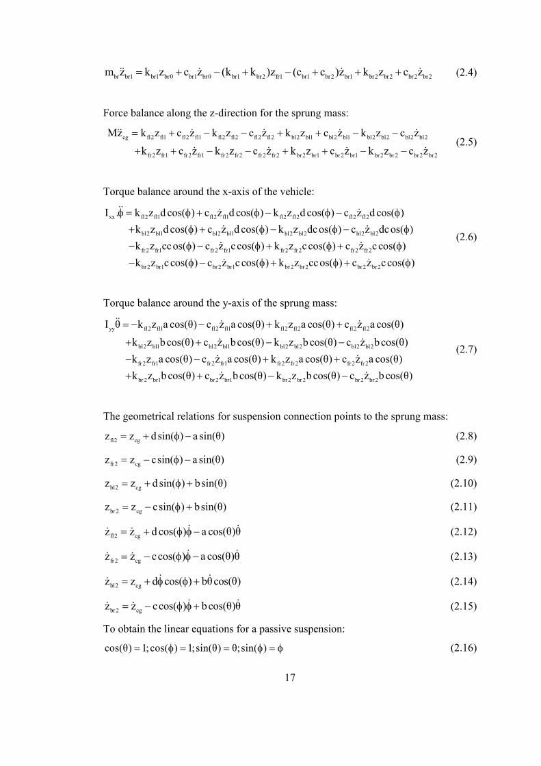
17

br br1 br1 br0 br1 br0 br1 br2 fr1 br1 br2 br1 br2 br2 br2 br2m z k z c z (k k )z (c c )z k z c z= + − + − + + +ɺɺ ɺ ɺ ɺ (2.4)

Force balance along the z-direction for the sprung mass:

cg fl2 fl1 fl2 fl1 fl2 fl2 fl2 fl2 bl2 bl1 bl2 bl1 bl2 bl2 bl2 bl2

fr2 fr1 fr2 fr1 fr2 fr2 fr2 fr2 br2 br1 br2 br1 br2 br2 br2 br2

Mz k z c z k z c z k z c z k z c z

k z c z k z c z k z c z k z c z

= + − − + + − −

+ + − − + + − −

ɺɺ ɺ ɺ ɺ ɺ

ɺ ɺ ɺ ɺ (2.5)

Torque balance around the x-axis of the vehicle:

xx fl2 fl1 fl2 fl1 fl2 fl2 fl2 fl2

bl2 bl1 bl2 bl1 bl2 bl2 bl2 bl2

fr2 fr1 fr2 fr1 fr2 fr2 fr2 fr2

I . k z d cos( ) c z d cos( ) k z d cos( ) c z d cos( )

k z d cos( ) c z d cos( ) k z dcos( ) c z dcos( )

k z ccos( ) c z ccos( ) k z ccos( ) c z c c

φ = φ + φ − φ − φ

+ φ + φ − φ − φ

− φ − φ + φ +

ɺɺ ɺ ɺ

ɺ ɺ

ɺ ɺ

br2 br1 br2 br1 br2 br2 br2 br2

os( )

k z c cos( ) c z c cos( ) k z ccos( ) c z ccos( )

φ

− φ − φ + φ + φɺ ɺ

(2.6)

Torque balance around the y-axis of the sprung mass:

yy fl2 fl1 fl2 fl1 fl2 fl2 fl2 fl2

bl2 bl1 bl2 bl1 bl2 bl2 bl2 bl2

fr2 fr1 fr2 fr1 fr2 fr2 fr2 fr2

I θ k z a cos(θ) c z a cos(θ) k z a cos(θ) c z a cos(θ)

k z bcos(θ) c z bcos(θ) k z b cos(θ) c z bcos(θ)

k z a cos(θ) c z a cos(θ) k z a cos(θ) c z a c

= − − + +

+ + − −

− − + +

ɺɺ ɺ ɺ

ɺ ɺ

ɺ ɺ

br2 br1 br2 br1 br2 br2 br2 br2

os(θ)

k z b cos(θ) c z bcos(θ) k z b cos(θ) c z b cos(θ)+ + − −ɺ ɺ

(2.7)

The geometrical relations for suspension connection points to the sprung mass:

fl2 cgz z dsin( ) a sin(θ)= + φ − (2.8)

fr2 cgz z csin( ) a sin(θ)= − φ − (2.9)

bl2 cgz z d sin( ) bsin(θ)= + φ + (2.10)

br2 cgz z csin( ) bsin(θ)= − φ + (2.11)

fl2 cgz z d cos( ) a cos(θ)θ= + φ φ−ɺ ɺɺ ɺ (2.12)

fr2 cgz z ccos( ) a cos(θ)θ= − φ φ−ɺ ɺɺ ɺ (2.13)

bl2 cgz z d cos( ) bθcos(θ)= + φ φ +ɺ ɺɺ (2.14)

br2 cgz z ccos( ) bcos(θ)θ= − φ φ+ɺ ɺɺ ɺ (2.15)

To obtain the linear equations for a passive suspension:

cos(θ) 1;cos( ) 1;sin(θ) θ;sin( )= φ = = φ = φ (2.16)

18

The geometrical relations become:

fr 2 cgz z c aθ= − φ− (2.17)

bl2 cgz z d bθ= + φ+ (2.18)

br2 cgz z c bθ= − φ+ (2.19)

fl2 cgz z d aθθ= + φφ−ɺ ɺɺ ɺ (2.20)

fr2 cgz z c aθθ= − φφ−ɺ ɺɺ ɺ (2.21)

bl2 cgz z d bθ= + φ+ɺ ɺɺ ɺ (2.22)

br2 cgz z c bθθ= − φφ+ɺ ɺɺ ɺ (2.23)

2.2.2 STATE SPACE REPRESENTATION OF THE LINEAR

PASSIVE SYSTEM

In the state space representation of the vehicle model with passive suspensions, all

equations of motion should be put in the form,

x Ax Cw= +ɺ (2.24)

where w represents the road disturbances:

[ ]T1 2 3 4 5 6 7 8w = w w w w w w w w

1 fl0 2 bl0 3 fr0 4 br0 5 bl0 6 bl0 7 bl0 8 bl0w = z ; w = z ; w = z ; w = z ; w = z ; w = z ; w = z ; w = zɺ ɺ ɺ ɺ

And x represents the state variables:

[ ]T1 2 3 4 5 6 7 8 9 10 11 12 13 14 x x x x x x x x x x x x x x x=

1 fl1 2 bl1 3 fr1 4 br1 5 cg 6 7

8 fl1 9 bl1 10 fr1 11 br1 12 cg 13 14

x = z ; x = z ; x =z ; x =z ; x =z ; x = ; x =θ

x = z ; x = z ; x =z ; x =z ; x =z ; x = ; x =θ

φ

φ ɺɺ ɺ ɺ ɺ ɺ

Derivatives will have " "ɺ and second derivates will have" "ɺɺ .

8 fl fl1 1 fl fl1 2 fl fl1 fl2 1 fl fl2 5

fl fl2 6 fl fl2 7 fl fl1 fl2 8

fl fl2 12 fl fl2 13 fl fl2 14

x 1/ m k .u 1/ m c .u 1/ m (k k ).x 1/ m k .x

1/ m k d x 1/ m k a x 1/ m (c c ).x

1/ m c .x 1/ m c d x 1/ m c a x

= + − + +

+ ⋅ − ⋅ − +

+ + ⋅ − ⋅

ɺ

(2.25)

19

9 bl bl1 3 bl bl1 4 bl bl1 bl2 2 bl bl2 5

bl bl2 6 bl bl2 7 bl bl1 bl2 9 bl blr2 12

bl blr2 13 bl blr2 14

x 1/ m k .u 1/ m c .u 1/ m (k k ).x 1/ m k .x

1/ m k d x 1/ m k b x 1/ m (c c ).x 1/ m c .x

1/ m c d x 1/ m c b x

= + − + +

+ ⋅ + ⋅ − + +

+ ⋅ + ⋅

ɺ

(2.26)

10 fr fr1 5 fr fr1 6 fr fr1 fr2 3 fr fr2 5

fr fr2 6 fr fr2 7 fr fr1 fr2 10 fr fr2 12

fr fr2 13 fr fr2 14

x 1/ m k .u 1/ m c .u 1/ m (k k ).x 1/ m k .x

1/ m k c x 1/ m k a x 1/ m (c c ) x 1/ m c x

1/ m c c x 1/ m c a x

= + − + +

− ⋅ − ⋅ − + ⋅ + ⋅

− ⋅ − ⋅

ɺ

(2.27)

11 br br1 7 br br1 8 br br1 br2 4 br br2 5

br br2 6 br br2 7 br br1 br2 11 br br2 12

br br2 13 br br2 14

x 1/ m k .u 1/ m c .u 1/ m (k k ).x 1/ m k .x

1/ m k c x 1/ m k b x 1/ m (c c ).x 1/ m c .x

1/ m c c x 1/ m c b x

= + − + +

− ⋅ + ⋅ − + +

− ⋅ + ⋅

ɺ

(2.28)

12 fl2 1 bl2 2 fr 2 3 br 2 4

fl2 bl2 fr 2 br 2 5

fl2 bl2 fr 2 br 2 6

fl2 bl2 fr 2 br 2 7 fl2 8 bl2 9

fr 2 10 br 2 11 f

x 1/ Mk x 1/ Mk x 1/ Mk x 1/ Mk x

1/ M( k k k k ) x

1/ M( k d k d k c k c) x

1/ M( k a k b k a k b) x 1/ M c .x 1/ M c x

1/ Mc x 1/ Mc .x 1/ M( c

= + ⋅ + ⋅ + ⋅ + ⋅

+ − − − − ⋅

+ − − + + ⋅

+ + − + − ⋅ + ⋅ + ⋅ ⋅

+ ⋅ + + −

ɺ

l2 bl2 br 2 br 2 12

fl2 bl2 fr 2 br 2 13

fl2 bl2 fr 2 br 2 14

c c c ).x

1/ M( c d c d c c c c) x

1/ M(c a c b c a c b) x

− − −

+ − − + + ⋅

+ − + − ⋅

(2.29)

13 yy fl2 1 yy bl2 2 yy fr2 3 yy br2 4

yy fl2 bl2 fr2 br2 5


2 2 2 2yy fl2 bl2 fr2 br2 7 yy fl2 8

yy bl2

x 1/ I k a x 1/ I k b x 1/ I k a x 1/ I k b x

1/ I (k a k b k a k b) x

1/ I (k ad k bd k ac k bc) x

1/ I ( k a k b k a k b ) x 1/ I c a x

1/ I c b x

= − ⋅ + ⋅ − ⋅ + ⋅

+ − + − ⋅

+ ⋅ − − + ⋅

+ − − − − ⋅ − ⋅

+ ⋅

ɺ

9 yy fr2 10 yy br2 11



2 2 2 2yy fl2 bl2 fr2 br2 14

1/ I c a x 1/ I c b x

1/ I (c a c b c a c b) x

1/ I (c ad c bd c ac c bc) x

1/ I ( c a c b c a c b ) x

− ⋅ + ⋅

+ − + − ⋅

+ − − + ⋅

+ − − − − ⋅

(2.30)

14 xx fl2 1 xx bl2 2 xx fr2 3 xx br2 4

xx fl2 bl2 fr2 br2 5

2 2 2 2xx fl2 bl2 fr2 br2 6


xx fl2 8 xx bl2

x 1/ I k d x 1/ I k d x 1/ I k c x 1/ I k c x

1/ I ( k d k d k c k c) x

1/ I ( k d k d k c k c ) x

1/ I ( k da k db k ca k cb) x

1/ I c d.x 1/ I c d

= + ⋅ + ⋅ − ⋅ − ⋅

+ − − + + ⋅

+ − − − − ⋅

+ + − − + ⋅

+ + ⋅

ɺ

9 xx fr2 10

xx br2 11 xx fl2 bl2 fr2 br2 12

2 2 2 2xx fl2 bl2 fr2 br2 13


x 1/ I c c x

1/ I c c x 1/ I ( c d c d c c c c) x

1/ I ( c d c d c c c c ) x

1/ I ( c da c db c ca c cb) x

− ⋅

− ⋅ + − − + + ⋅

+ − − − − ⋅

+ + − − + ⋅

(2.31)

20

2.2.3 EQUATIONS OF MOTION IN STATE SPACE FORM

[ ]11 12 13 14 15A A A A A A=

11 fl1 fl2 fl

bl1 bl2 bl

fr1 fr2 fr

br1 br2

br

fl2 bl2 fr2 br2

fl2 yy bl2 yy fr2 yy br2 yy

fl2 xx bl2 xx fr2 xx b

0 0 0 0

0 0 0 0

0 0 0 0

0 0 0 0

0 0 0 0

0 0 0 0

0 0 0 0

A (k k ) / m 0 0 0

0 (k k ) / m 0 0

0 0 (k k ) / m 0

(k k )0 0 0

m

k / M k / M k / M k / M

k a / I k b / I k a / I k b / I

k d / I k d / I k c / I k

= − +

− +

− +

+−

− −

− − r2 xxc / I

(2.32)

12

fl fl2 fl fl2

bl bl2 bl bl2

fr fr 2 fr fr 2

br br 2 br br 2

fl2 bl2 fr 2 br 2 fl2 bl2 fr 2

fl2 bl2 fr 2 br 2 yy

fl2 bl2 fr 2 br 2 xx

0 0

0 0

0 0

0 0

0 0

0 0

0 0A

1/ m k 1/ m k d

1/ m k 1/ m k d

1/ m k 1/ m k c

1/ m k 1/ m k c

(k k k k ) / M ( k d k d k c

(k a k b k a k b) / I

( k d k d k c k c) / I

=

−

+ −

− + + + − − + +

− + −

− − + +

br 2

fl2 bl2 fr 2 br 2 yy

2 2 2 2fl2 bl2 fr 2 br 2 xx

k c) / M

(k ad k bd k ac k bc) / I

( k d k d k c k c ) / I

− − + − − − −

(2.33)

21

fl1 fl2fl fl213

fl

bl1 bl2bl bl2

bl

fr fr 2

br br 2

fl2 bl2 fr 2 br 2 fl2 bl2

2 2 2 2fl2 bl2 fr2 br 2 yy fl2 yy bl2 yy

0 1 0

0 0 1

0 0 0

0 0 0

0 0 0

0 0 0

0 0 0

(c c )1/ m k a 0A

m

(c c )1/ m k b 0

m

1/ m k a 0 0

1/ m k b 0 0

1/ M ( k a k b k a k b) c / M c / M

( k a k b k a k b ) / I c a / I bc / I

(

+− −=

+−

−

+

⋅ + − + −

− − − − −

fl2 bl2 fr 2 br 2 xx fl2 xx bl2 xxk da k db k ca k cb) / I c d / I c d / I

+ − − +

(2.34)

14

fl2 fl

bl2 fl

bl1 bl2 bl fr2 fl

br1 br2 br br2 fl

fl2 br2 fl2 bl2 bl2 br2

fr2 yy br2 yy br2 fr2 bl2 fl2 yy

fr2 xx br2 x

0 0 0

0 0 0

1 0 0

0 1 0

0 0 1

0 0 0

0 0 0A

0 0 c / m

0 0 c / m

(c c ) / m 0 c / m

0 -(c c ) / m c / m

c / M c / M (c c c c ) / M

- ac / I bc / I (-bc ac - bc ac ) / I

-c c / I -c c / I

=

− +

+

− + + +

+ +

x bl2 fl2 br2 fr2 xx(-c d - c d c c c c) / I

+ +

(2.35)

22

fl2 fl2

f l fl

bl2 bl2

15 fl fl

fr2 fr2

fl fl

br2 br2

fl fl

bl2 fl2 br 2 fr2 br2 fr2 bl2 fl2

2 2 2 2fl2 fr2 br2 bl2 fr2 fl2 br2

yy

0 0

0 0

0 0

0 0

0 0

1 0

0 1

c d c a

m m

c d c b

A m m

c c c a

m m

c c c b

m m

-c d - c d c c c c) (-bc ac - bc ac )(

M M

(-ac d ac c - bc c bc d) -(a c a c b c b c-

I

−

=

− −

−

+ + + +

+ + + + + bl2

yy

2 2 2 2fr2 br2 fl2 bl2 fl2 fr2 br2 bl2

xx xx

)

I

-(c c c c c d c d ) -(-ac d ac c - bc c bc d)

I I

+ + + + +

(2.36)

23

[ ]11 12C C C=

11

fl fl1

bl bl1

fr fr1

br br1

0 0 0 0

0 0 0 0

0 0 0 0

0 0 0 0

0 0 0 0

0 0 0 0

0 0 0 0C

1/ m k 0 0 0

0 1/ m k 0 0

0 0 1/ m k 0

0 0 0 1/ m k

0 0 0 0

0 0 0 0

0 0 0 0

=

(2.37)

12

fl fl1

bl bl1

fr fr1

br br1

0 0 0 0

0 0 0 0

0 0 0 0

0 0 0 0

0 0 0 0

0 0 0 0

0 0 0 0C

1/ m c 0 0 0

0 1/ m c 0 0

0 0 1/ m c 0

0 0 0 1/ m c

0 0 0 0

0 0 0 0

0 0 0 0

=

(2.38)

24

2.2.4 STATE SPACE REPRESENTATION OF THE LINEAR

SEMI-ACTIVE SYSTEM

The state space representation of a semi-active suspension is different than passive

suspension since the damping coefficients are variable. To overcome this difficulty a

state space representation of the form described below will be used.

x=Ax+Bw+Cuɺ (2.39)

The state variables and the disturbances are defined in the same manner like in

section 2.2.3 where u represents the semi-active damping forces in the system:

Tdamperfl damperbl damperfr damperbru = F F F F (See list of symbols)

The equations become:

8 fl fl0 1 fl fl1 5 fl fl1 fl2 1 fl fl2 5

fl fl2 6 fl fl2 7 fl fl1 8 fl damperfl

x 1/ m k .u 1/ m c .u 1/ m (k k ).x 1/ m k .x

1/ m k d x 1/ m k a x 1/ m c .x 1/ m .F

= + − + +

+ ⋅ − ⋅ − +

ɺ

(2.40)

9 bl bl1 2 bl bl1 6 bl bl1 bl2 2 bl bl2 5

bl bl2 6 bl bl2 7 bl bl1 9 bl damperbl

x 1/ m k .u . 1/ m c .u 1/ m (k k ).x 1/ m k .x

1/ m k d x 1/ m k b x 1/ m c .x 1/ m F

= + − + +

+ ⋅ + ⋅ − + ⋅

ɺ

(2.41)

10 fr fr1 3 fr fr1 7 fr fr1 fr 2 3 fr fr2 5

fr fr2 6 fr fr2 7 fr fr1 10 fr damperfr

x 1/ m k .u . 1/ m c .u 1/ m (k k ).x 1/ m k .x

1/ m k c x 1/ m k a x 1/ m c .x 1/ m F

= + − + +

− ⋅ − ⋅ − + ⋅

ɺ

(2.42)

10 fr fr1 3 fr fr1 7 fr fr1 fr2 3 fr fr2 5

fr fr2 6 fr fr2 7 fr fr1 10 fr damperfr

x 1/ m k .u 1/ m c .u 1/ m (k k ).x 1/ m k .x

1/ m k c x 1/ m k a x 1/ m c x 1/ m F

= + − + +

− ⋅ − ⋅ − + ⋅

ɺ

(2.43)

11 br br1 4 br br1 8 br br1 br2 4 br br2 5

br br2 6 br br2 7 br br1 11 br damperbr

x 1/ m k .u 1/ m c .u 1/ m (k k ).x 1/ m k .x

1/ m k c x 1/ m k b x 1/ m c .x 1/ m F

= + − + +

− ⋅ + ⋅ − + ⋅

ɺ

(2.44)

12 fl2 1 bl2 2 fr2 3 br2 4

fl2 bl2 fr2 br2 5

fl2 bl2 fr2 br2 6

fl2 bl2 fr2 br2 7 damperfl

damperbl damperfr damperbr

x 1/ Mk x 1/ Mk x 1/ Mk x 1/ Mk x

1/ M( k k k k ) x

1/ M( k d k d k c k c) x

1/ M( k a k b k a k b) x 1/ M F

1/ M F 1/ M F 1/ M F

= + ⋅ + ⋅ + ⋅ + ⋅

+ − − − − ⋅

+ − − + + ⋅

+ + − + − ⋅ − ⋅

− ⋅ − ⋅ − ⋅

ɺ

(2.45)

25

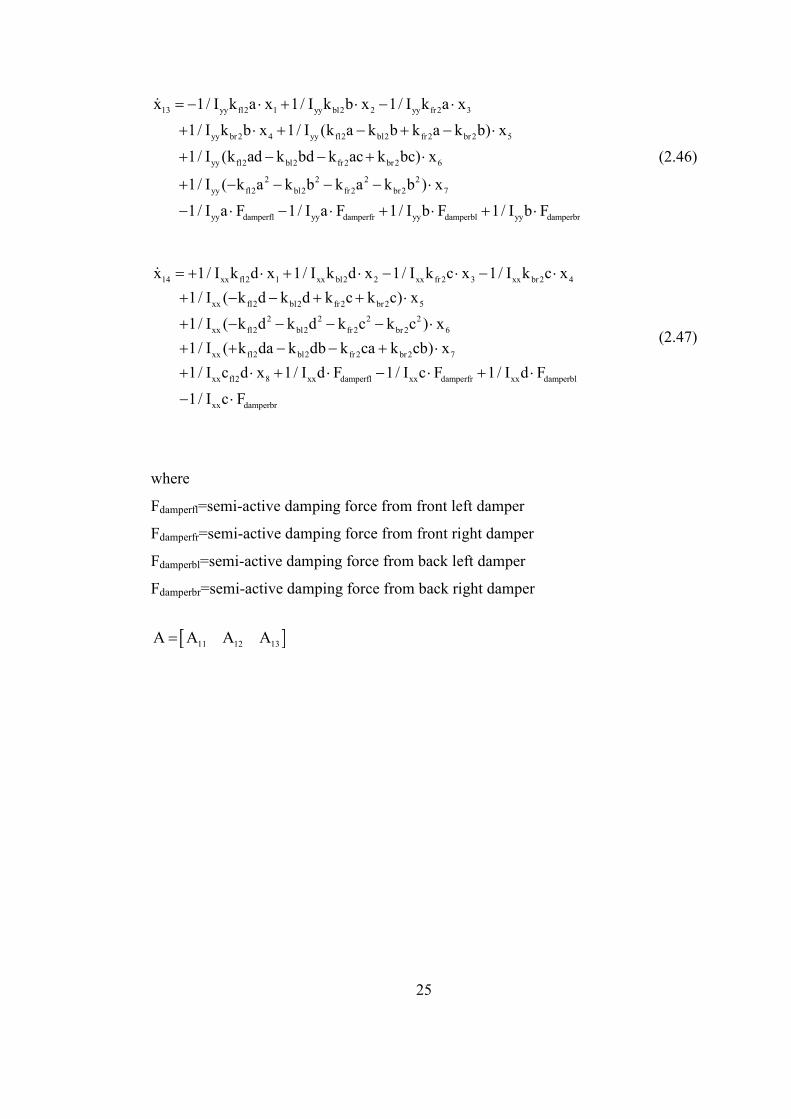
13 yy fl2 1 yy bl2 2 yy fr2 3

yy br2 4 yy fl2 bl2 fr2 br2 5


2 2 2 2yy fl2 bl2 fr2 br2 7

yy damperfl yy da

x 1/ I k a x 1/ I k b x 1/ I k a x

1/ I k b x 1/ I (k a k b k a k b) x

1/ I (k ad k bd k ac k bc) x

1/ I ( k a k b k a k b ) x

1/ I a F 1/ I a F

= − ⋅ + ⋅ − ⋅

+ ⋅ + − + − ⋅

+ − − + ⋅

+ − − − − ⋅

− ⋅ − ⋅

ɺ

mperfr yy damperbl yy damperbr1/ I b F 1/ I b F+ ⋅ + ⋅

(2.46)

14 xx fl2 1 xx bl2 2 xx fr2 3 xx br2 4


2 2 2 2xx fl2 bl2 fr2 br2 6


xx fl2 8 xx dam

x 1/ I k d x 1/ I k d x 1/ I k c x 1/ I k c x

1/ I ( k d k d k c k c) x

1/ I ( k d k d k c k c ) x

1/ I ( k da k db k ca k cb) x

1/ I c d x 1/ I d F

= + ⋅ + ⋅ − ⋅ − ⋅

+ − − + + ⋅

+ − − − − ⋅

+ + − − + ⋅

+ ⋅ + ⋅

ɺ

perfl xx damperfr xx damperbl

xx damperbr

1/ I c F 1/ I d F

1/ I c F

− ⋅ + ⋅

− ⋅

(2.47)

where

Fdamperfl=semi-active damping force from front left damper

Fdamperfr=semi-active damping force from front right damper

Fdamperbl=semi-active damping force from back left damper

Fdamperbr=semi-active damping force from back right damper

[ ]11 12 13A A A A=

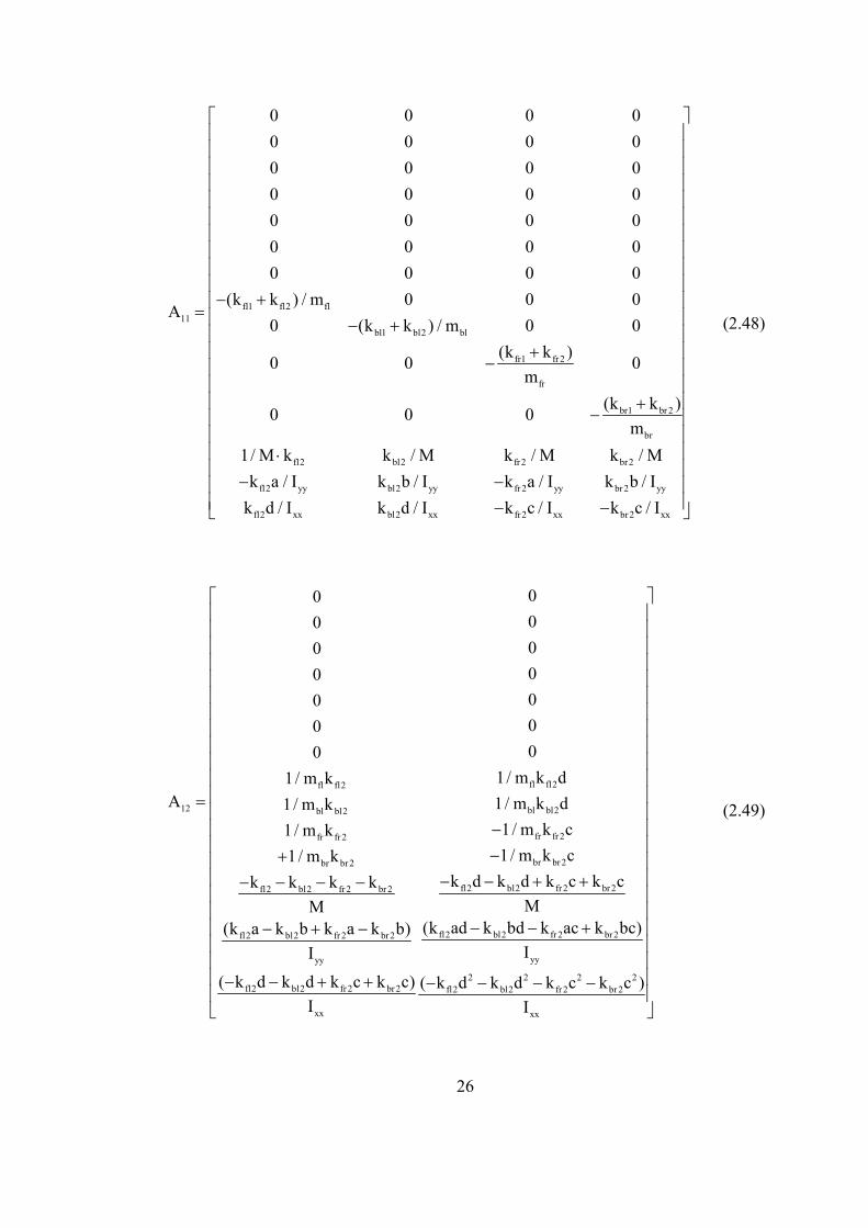
26

fl1 fl2 fl11

bl1 bl2 bl

fr1 fr2

fr

br1 br2

br

fl2 bl2 fr2 br2

fl2 yy bl2 yy fr2 yy br2 yy

fl2 xx bl2 xx fr2 xx

0 0 0 0

0 0 0 0

0 0 0 0

0 0 0 0

0 0 0 0

0 0 0 0

0 0 0 0

(k k ) / m 0 0 0A

0 (k k ) / m 0 0

(k k )0 0 0

m

(k k )0 0 0

m

1/ M k k / M k / M k / M

k a / I k b / I k a / I k b / I

k d / I k d / I k c / I k

− +=

− +

+−

+−

⋅

− −

− − br2 xxc / I

(2.48)

fl fl2fl fl2

12 bl bl2bl bl2

fr fr 2fr fr 2

br br 2br br 2

fl2 bl2 fr 2 br 2fl2 bl2 fr 2 br 2

fl2 bl2 fr 2 br 2

yy

fl2 bl2 fr 2 br 2

xx

00

00

00

00

00

00

00

1/ m k d1/ m kA 1/ m k d1/ m k

1/ m k c1/ m k

1/ m k c1/ m k

k d k d k c k ck k k k

MM(k a k b k a k b)

I

( k d k d k c k c)

I

=

−

−+

− − + +− − − −

− + −

− − + +

fl2 bl2 fr 2 br 2

yy

2 2 2 2fl2 bl2 fr 2 br 2

xx

(k ad k bd k ac k bc)

I

( k d k d k c k c )

I

− − + − − − −

(2.49)

27

fl fl2

13bl bl2

fr fr 2

br br 2

fl2 bl2 fr 2 br 2

2 2 2 2fl2 bl2 fr 2 br 2

yy

0 1 0 0 0 0 0 0

0 0 1 0 0 0 0 0

0 0 0 1 0 0 0 0

0 0 0 0 1 0 0 0

0 0 0 0 0 1 0 0

0 0 0 0 0 0 1 0

0 0 0 0 0 0 0 1

1/ m k a 0 0 0 0 0 0 0A

1/ m k b 0 0 0 0 0 0 0

1/ m k a 0 0 0 0 0 0 0

1/ m k b 0 0 0 0 0 0 0

1/ M(k a k b k a k b) 0 0 0 0 0 0 0

( k a k b k a k b )

I

−=

−

+

− + −

− − − −

fl2 bl2 fr2 br 2

xx

0 0 0 0 0 0 0

(k da k db k ca k cb)0 0 0 0 0 0 0

I

− − +

(2.50)

B matrix

fl fl1

bl bl1

fr fr1

br br1

0 0 0 0 0 0 0 0

0 0 0 0 0 0 0 0

0 0 0 0 0 0 0 0

0 0 0 0 0 0 0 0

0 0 0 0 0 0 0 0

0 0 0 0 0 0 0 0

0 0 0 0 0 0 0 0B

1/ m k 0 0 0 0 0 0 0

0 1/ m k 0 0 0 0 0 0

0 0 1/ m k 0 0 0 0 0

0 0 0 1/ m k 0 0 0 0

0 0 0 0 0 0 0 0

0 0 0 0 0 0 0 0

0 0 0 0 0 0 0 0

=

(2.51)

28

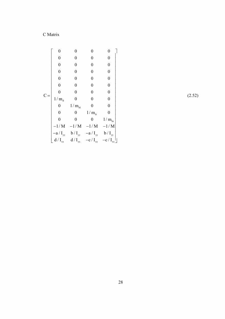
C Matrix

fl

bl

fr

br

yy yy yy yy

xx xx xx xx

0 0 0 0

0 0 0 0

0 0 0 0

0 0 0 0

0 0 0 0

0 0 0 0

0 0 0 0C

1/ m 0 0 0

0 1/ m 0 0

0 0 1/ m 0

0 0 0 1/ m

1/ M 1/ M 1/ M 1/ M

a / I b / I a / I b / I

d / I d / I c / I c / I

= − − − − − − − −

(2.52)

29

CHAPTER 3

3 SEMI-ACTIVE CONTROL STRATEGY

3.1 INTRODUCTION

The semi-active damping control concept is illustrated in Figure 3.1. The 7-dof

vehicle model has four force inputs from MR dampers and four disturbance inputs

from the road surface profile. The states of the seven degree of freedom model are

assumed to be measured or estimated and then fed back to the controller. The

controller determines required damper forces needed for a chosen control strategy.

The MR dampers should then be actuated by proper currents that will generate the

MR damping force inputs determined by the controller. After required currents are

calculated, MR dampers are actuated by these. In this work, the currents to provide

the desired damping forces are assumed to be correctly determined as long as the

forces are in the feasible damping range.

The control strategy is chosen as Linear Quadratic Regulator (LQR) and it will be

discussed in the next pages.

Figure

3.2 SENSOR

The selected LQR control

seven degrees of freedom vehicle model

freedoms and related

etc.) are needed to be fed back to the controller in order to determine the necessary

damper input currents. Thus, four accelerometers for tires and an IM

measuring unit) with one accelerometer and a three

four accelerometers should be mounted on wheel hubs to measure unsprung mass

accelerations. The IMU

of the vehicle to determine

computation. It can also be placed at other locations of the vehicle.

control, wire type linear displacement transducers (LDT) are also used to determine

rattle space displacement

displacements can also be derived from the unsprung mass accelerometers, but for

greater accuracy, LDTs are utilized. Following the measurement of these degrees of

freedoms, necessary calculations such as integration are performed to obtain

states which will be fed back.

30

igure 3.1 Semi-Active Damper Control Concept

REQUIREMENTS

control strategy controls bounce, pitch and roll

of freedom vehicle model. Fourteen states, which are degree

freedoms and related inputs (such bounce rate and bounce, roll rate and roll angle


damper input currents. Thus, four accelerometers for tires and an IM

measuring unit) with one accelerometer and a three-axes gyroscope are needed. The


The IMU and the accelerometer can be placed at the center of gravity

to determine roll, and pitch rates (yaw axis is neglected)

computation. It can also be placed at other locations of the vehicle.

type linear displacement transducers (LDT) are also used to determine

displacement changes (Choi, Han, Song, & Choi, 2007)



ary calculations such as integration are performed to obtain

states which will be fed back.

Active Damper Control Concept

pitch and roll motions of the

ich are degrees of

and bounce, roll rate and roll angle


damper input currents. Thus, four accelerometers for tires and an IMU (Inertial

axes gyroscope are needed. The


be placed at the center of gravity

roll, and pitch rates (yaw axis is neglected) for easy

computation. It can also be placed at other locations of the vehicle. For skyhook

type linear displacement transducers (LDT) are also used to determine

Choi, Han, Song, & Choi, 2007). The rattle space



ary calculations such as integration are performed to obtain fourteen

31

3.3 MR MODELLING

In the simulations to be carried, Matlab/Simulink will be used so that the empirically

obtained characteristics of MR dampers are simulated via lookup-tables which do not

rely on parametric or nonparametric models. Since the interpolation will be carried

between adjacent characteristics points, the characteristics are sampled as data points

from the experimental plots of characteristics curves by the help of a data

digitalization program. The sampling rate of the data points should be fine enough in

order to provide good accuracy and enable feasible computational time

simultaneously. One can set the interpolation linear or quadratic as a Matlab lookup-

tables property. In the simulations throughout the thesis work, inverse modelling to

find necessary current inputs to generate desired damping forces is not used. The

limits of the damping forces at a specified relative velocity across suspension are

used as the feasible damping range. However, in the implementation of the control

system or to be used in hardware in the loop simulations, inverse modelling will be

required. The necessary current input may then be determined by an Embedded M-

file block whose code is given in APPENDIX A. The Simulink block used for

calculating the current to generate desired damping force uses interpolation. This

interpolation is made between data points at the same relative velocity but at

different current levels to find the right input current for the required control input.

The MR characteristics used is given at APPENDIX E. The MR damper

characteristics used is selected considering the vehicle parameters in APPENDIX B

and existing dampers in section 1.3.1.2 in the light of the selection guide in section

1.3.1.2.

3.4 OPTIMAL CONTROL/ LINEAR QUADRATIC

REGULATOR CONTROL STRATEGY

In the case of full car ride model there are seven degrees of freedom which is

affected by four inputs from the road surface. In the case of controlling more than

one parameter as in the case of the scope of this thesis, developing a control strategy

32

is a tedious task. The control inputs should be chosen according to physical

constraints in the controlled plant and the semi-active damper force limitations.

Optimal control gives a systematic approach to solving this problem to minimize

chosen performance criterion (performance index or cost function) while the

equations of motion of the vehicle are satisfied. However when the control force

inputs are semi-active damper forces present in the vehicle, additional control

algorithms should be added to optimal control to satisfy semi-active damper physical

constraints. These additional control algorithms are discussed at 3.4.3.

3.4.1 A THEORETICAL LOOK INTO LINEAR QUADRATIC

REGULATOR CONTROL STRATEGY

The linear quadratic regulator is an optimal control problem where the plant state

equations are linear, the cost function is quadratic, and the test conditions consist of

random initial conditions and random disturbance inputs (B.Burl, 1999). The linear,

time invariant plant state equation is written as

( ) ( ) ( )x t Ax t Bw t Cu(t)= + +ɺ (3.1)

where x is the vector of states in the full ride vehicle model, u is the semi-active

damping forces, and w is the random road disturbances.

In the quadratic cost function of the type (Sinha, 2007):

( ) ( ) ( ) ( )T T T

0

J (x t Qx t u t Ru t 2x Nu(t))dt∞

= + +∫ (3.2)

where Q is a symmetric, a positive semi definite matrix and R is a symmetric

positive definite matrix. N is also positive a definite matrix.

The solution of the optimal control becomes (Naidu, 2003):

( ) ( )1 T Tu t R (B S N )x t−= − + (3.3)

where S is the solution of Algebraic Riccati Equation

T TA XS XSS X 0S Q+ − + = (3.4)

In the thesis the cost function is:

33

2 2 2 2 2 2 21 cg 2 3 4 damperfl damperfr damperbl damperbr

0

J [ (z ) ( ) ( ) (F F F F )]dt∞

= ρ + ρ θ +ρ φ +ρ + + +∫ ɺɺ (3.5)

where ρ1, ρ2, ρ3, ρ4 are weighting constants determined by trial and error process.

The constant ρ4 applies to the damping force inputs from four separate MR dampers.

3.4.2 THE LIMITATIONS OF TIME-INVARIANT LINEAR

QUADRATIC REGULATOR

The limitations of the time invariant LQR control strategy to be stable and have a

solution are given in (Matlab R2007b -The Language of Technical Computing, n.d.)

as follows:

1-The pair (A, C) should be stabilizable.

2-R>0 and Q-NR-1NT ≥0

3- (Q-NR-1NT, A- CR-1NT) has no unobservable mode on the imaginary axis.

The first condition holds for the system matrices A and C derived in section 2.2.4 for

the vehicle data specified in APPENDIX B. All the modes are stable. The other

criterions are to be checked for different cost functions. In this work Matlab (Matlab

R2007b -The Language of Technical Computing, n.d.) is used to determine full state

feedback gain matrix (K) . After specifying weighting factors; Q, R, and N matrices

are computed and fed to Matlab. The computation of a full state feedback matrix (K)

solution is only possible when all these criterions are met.

3.4.3 FEASIBILITY OF LQR C

ACTIVE DAMPERS

The required damping forces determined by the controller are not alway

since the forces do not lie in the admissible force region of the damper shown at

Figure 3.2.The forces applicable at a certain relative velocity should be between the

maximum force and the minimum force tha

supplied.

If it were an ideal active system that has the capability to give right damping forces,

the linear quadratic controller would work perfectly.

Figure 3.2 Admissible Damping Region

34

FEASIBILITY OF LQR CONTROL INPUTS FOR SE

ACTIVE DAMPERS

The required damping forces determined by the controller are not alway


.The forces applicable at a certain relative velocity should be between the

maximum force and the minimum force that can be attained by changing the current


the linear quadratic controller would work perfectly.

Admissible Damping Region of a Typical Semi-Active Damper

ONTROL INPUTS FOR SEMI-

The required damping forces determined by the controller are not always feasible


.The forces applicable at a certain relative velocity should be between the

t can be attained by changing the current


Active Damper

35

Possible approaches for this problem in feasibility of LQR inputs are discussed in the

next section:

3.4.3.1 Constrained Optimal Control

The main constraint in LQR control for semi-active dampers is that the damping

coefficient cannot be negative and cannot exceed some values. The work by

(Butsuen, 1989) formulated a constrained optimal control problem for a full car ride

model. He concluded that the difference in performance between clipped and

constrained optimal control is negligible.

The constrained optimal control problem becomes very complicated to solve for full

car ride models since it is a relatively complex model. The clipped optimal control

will be discussed in the next section as a potential solution.

3.4.3.2 Clipped Optimal Control

Clipped optimal control makes sure that if the desired force from the controller is in

the admissible region then it is applied by the MR dampers. If it is outside the region,

the control input forces are clipped to give the closest damping force to the desired

input as much as possible. The process is illustrated in Figure 3.3.

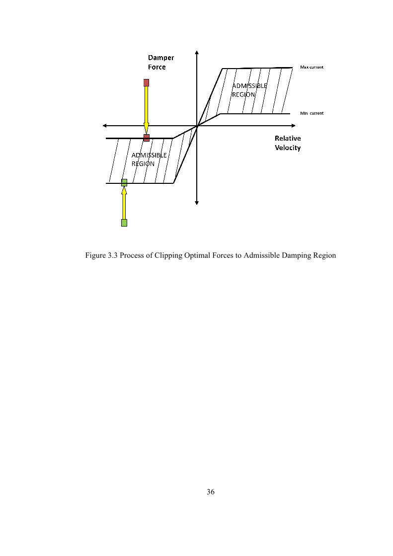
Figure 3.3 Process

36

Process of Clipping Optimal Forces to Admissible Damping Region

Admissible Damping Region

37

First of all the set of weighting constants that will be used in the quadratic

performance index given in equation 3.6 is chosen.

2 2 2 2 2 2 21 cg 2 3 4 damperfl damperfr damperbl damperbr

0

J [ρ (z ) ρ (θ) ρ ( ) ρ (F F F F )]dtφ∞

= + + + + + +∫ ɺɺ

(3.6)

This cost function index with the weighting constants is equivalent to the expression

( ) ( ) ( ) ( )T T T

0

J (x t Qx t u t Ru t 2x Nu(t))dt∞

= + +∫

(3.7)

Then the Q, R, and N matrices in the equivalent performance index are determined

by considering the equations of motion of the seven degree of freedom vehicle

model. The state space representation used in the cost function was determined at

section 2.2.4. Afterwards the necessary states are collected and the full state feedback

is computed by the LQR strategy while simulating the response of the vehicle to road

inputs. The closest damping force lying in the admissible region to the required

optimal force is determined and taken from the damper.

The weighting constants used in the cost function should be tuned. This tuning needs

an iteration process on different road conditions. From the simulations based on

specific road profiles, the weighting constants should be decided on user preference

to give emphasis to which parameter to be minimized. The tuning process must begin

with initial guesses. To make the initial guess properly, the response to an input of

the vehicle model with passive suspension should be examined. The scalar values of

the parameters in the performance index can be set proportionally by just examining

the values. As an example, the vehicle whose data is given at APPENDIX B can be

simulated over a road bump. From the results if one tries to minimize the bounce

acceleration, pitch angle or roll angle at the same importance level, one can start with

the weighting factor set of 8 4 41 2 3 4ρ 10 ; ρ 10 ; ρ 10 ; ρ 1= = = =

38

3.4.3.3 Optimal Gain Switching Control

The main methodology is proposed by (Giua, Seatzu, & Usai, 1999). As mentioned

in the literature survey, Section 1.4, Optimal Gain Switching method gives a

bounded target control force by switching between different feedback gains. There

exists two phases for the design. The cost function used in this strategy is as follows:

( ) ( ) ( ) ( )T Tm

0

(ρx t Q x t +v t Rv t )dt∞

∫

(3.8)

In the first phase, the Qm and R matrices are constants which are decided by

intuition, v(t) is the control input, and ρ is the controlled parameter to design a good

active suspension control law that will later be mimicked by the semi-active

suspension. When the system is far from the origin, low ρ should be used and when

the system is close to the origin large ρ can be used in order to satisfy the constraint

that the semi-active the magnitude of damping force cannot exceed a limit. This

method also calculates the region of state space in which the control forces are

bounded. The initial conditions that the system can have without violating the

constraint are analyzed for every ρ and stored as data. In the simulation, the largest ρ

that will cause the damping force satisfying the force magnitude constraint is chosen.

Then the force is the target control force is approximated by controlling the damper

coefficient.

The most complex part of this theory is calculating the initial conditions that will

satisfy the force magnitude constraint. If the work were to be carried on quarter car

model, the computing power would be adequate. However the computation difficulty

for 7 degree of freedom full-car ride model is a very serious complication.

39

3.5 SKYHOOK, GROUNDHOOK CONTROL

STRATEGY

These control strategies are simple but also effective in controlling the body bounce

motion. They are based on quarter car models and are not specially designed to

control pitch and roll motions. Skyhook control strategy is effective on reducing

sprung mass bounce acceleration and groundhook control strategy is very effective at

unsprung mass acceleration (Ahmadian M. P., 2000). Skyhook control strategy

applies damping force proportional to sprung mass velocity whereas groundhook

control strategy applies damping force proportional to unsprung mass velocity. Both

of these try to give no damping force depending on the sign of the relative velocity of

the damper ends, specified by the particular methodology described in equations 3.9-

12. The notation used for the quarter car model can be seen in Figure 3.4. A

combination of the skyhook and groundhook methods is also commonly used and

called hybrid control. In hybrid control, damping forces computed by skyhook and

groundhook controls are added in a proportion determined by the designer. Hybrid

control is a compromise between two classical strategies in minimizing sprung and

unsprung mass motions.

Skyhook control strategy is widely used in present applications. There are also

constraints in the skyhook control strategy. As in the LQR optimal control the

requested force is clipped towards the damper capability. For minimal damping

force, no current is supplied to the damper. However it still provides some damping.

If the requested damper force is larger than the maximum possible damping force,

the maximum input current is supplied to the damper. If the force is between the

limits, the requested force can be applied.

40

Classical Skyhook Control Strategy:

damper s 2 2 2 1

damper 2 2 1

F G z if z (z z ) 0

F 0 if z (z z ) 0

= − >

= − ≤

ɺ ɺ ɺ ɺ

ɺ ɺ ɺ (3.9)

Groundhook Control strategy:

damper g 1 1 2 1

damper 1 2 1

F G z if z (z z ) 0

F 0 if z (z z ) 0

= − <

= − ≥

ɺ ɺ ɺ ɺ

ɺ ɺ ɺ (3.10)

Hybrid Control Strategy:

(3.11)

where

skyhook s 2 2 2 1

skyhook 2 2 1

groundhook g 1 1 2 1

groundhook 1 2 1

σ G z if z (z z ) 0

σ 0 if z (z z ) 0

σ G z if z (z z ) 0

σ 0 if z (z z ) 0

= − >

= − ≤

= − <

= − ≥

ɺ ɺ ɺ ɺ

ɺ ɺ ɺ

ɺ ɺ ɺ ɺ

ɺ ɺ ɺ

(3.12)

Figure 3.4 Quarter Car Model

damper sky groundhookF ασ (1 α)σ= + −

1z

0blz

1c

2k

1k

um

sm

2z

damperF

41

CHAPTER 4

4 SIMULATION MODEL

4.1 SIMULINK MODEL

The simulation model and its graphical user interface are constructed using Matlab.

In the Simulink model, nonlinear seven degree of freedom ride model is built. Its

general structure is given in the Appendix A. The equations used to build the

Simulink model have been given in chapter 2. The main difference of the model from

a normal ride model is the additional embedded semi-active suspensions. The

Simulink model should contain an MR damper model and the block sets to control

the dampers independently. The MR damper models consist of lookup tables and the

block sets to control the dampers. The control blocks are built for optimal control. In

addition to optimal control blocks, the skyhook control blocks are also constructed

for comparison purposes between skyhook and optimal control. These blocks are

given at the next section.

4.2 OPTIMAL CONTROLLER BLOCKS

The optimal control blocks consist of products of the system states and the feedback

gains computed before the simulations. The optimal control block of front left

damper is illustrated in Figure 4.1

However the computed force for optimal control is not always feasible, so the block

given in Figure 4.2 should also be embedded. If the requested damping force is

outside the admissible damping region, the control input forces are redetermined to

42

give the closest damping force to the desired input as much as possible. If the desired

force is between the bounds of the available damping forces, no modification is done.

Figure 4.1 Full State Feedback Optimal Control Simulink Model

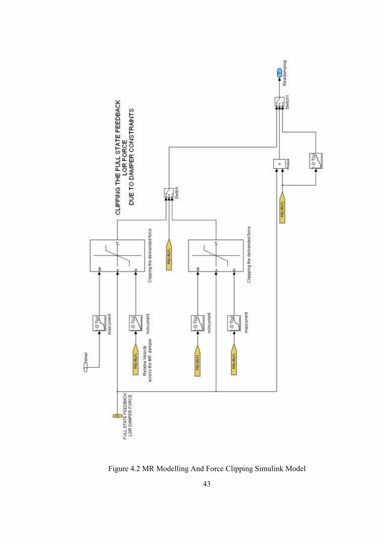
43

Figure 4.2 MR Modelling And Force Clipping Simulink Model

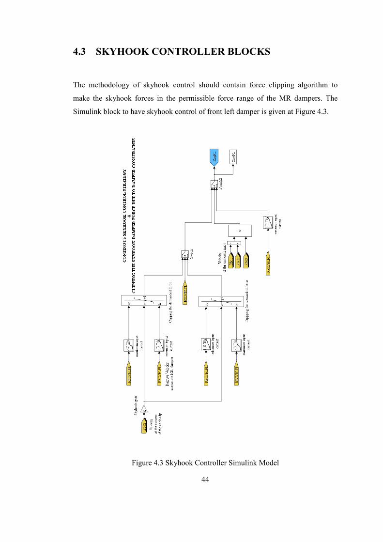
44

4.3 SKYHOOK CONTROLLER BLOCKS

The methodology of skyhook control should contain force clipping algorithm to

make the skyhook forces in the permissible force range of the MR dampers. The

Simulink block to have skyhook control of front left damper is given at Figure 4.3.

Figure 4.3 Skyhook Controller Simulink Model

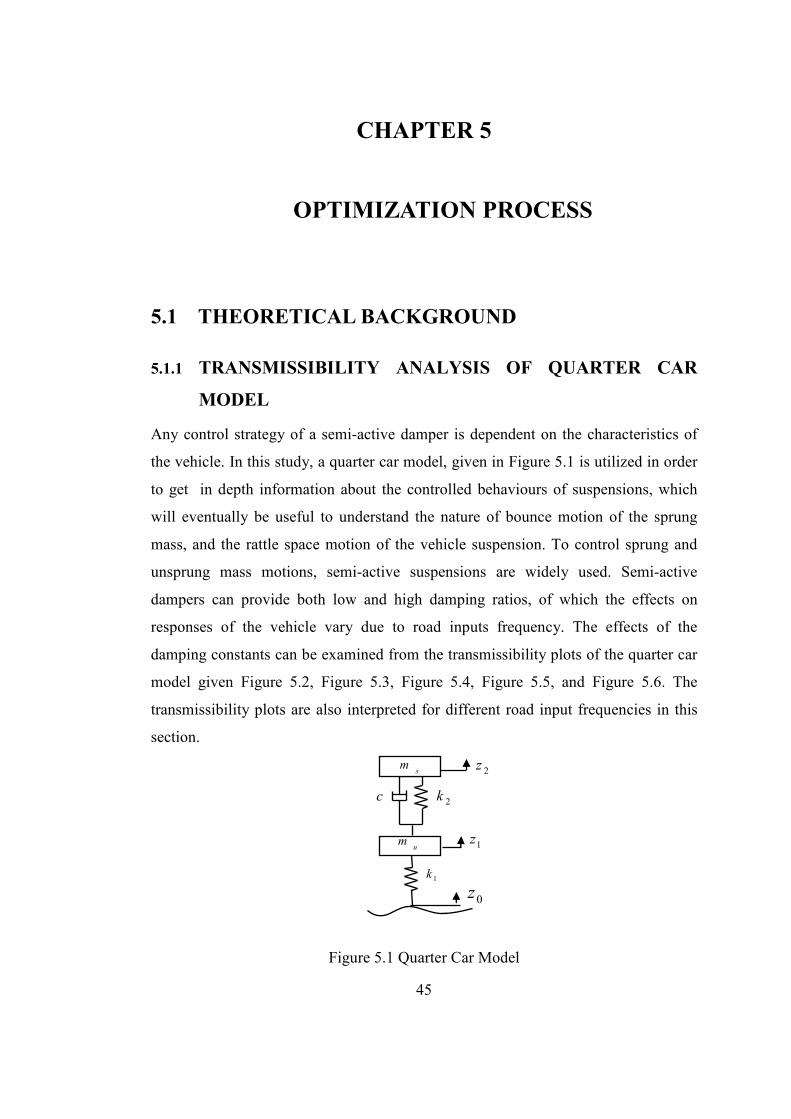
45

CHAPTER 5

5 OPTIMIZATION PROCESS

5.1 THEORETICAL BACKGROUND

5.1.1 TRANSMISSIBILITY ANALYSIS OF QUARTER CAR

MODEL

Any control strategy of a semi-active damper is dependent on the characteristics of

the vehicle. In this study, a quarter car model, given in Figure 5.1 is utilized in order

to get in depth information about the controlled behaviours of suspensions, which

will eventually be useful to understand the nature of bounce motion of the sprung

mass, and the rattle space motion of the vehicle suspension. To control sprung and

unsprung mass motions, semi-active suspensions are widely used. Semi-active

dampers can provide both low and high damping ratios, of which the effects on

responses of the vehicle vary due to road inputs frequency. The effects of the

damping constants can be examined from the transmissibility plots of the quarter car

model given Figure 5.2, Figure 5.3, Figure 5.4, Figure 5.5, and Figure 5.6. The

transmissibility plots are also interpreted for different road input frequencies in this

section.

Figure 5.1 Quarter Car Model

1z

0z

2k

1k

um

sm

2z

c

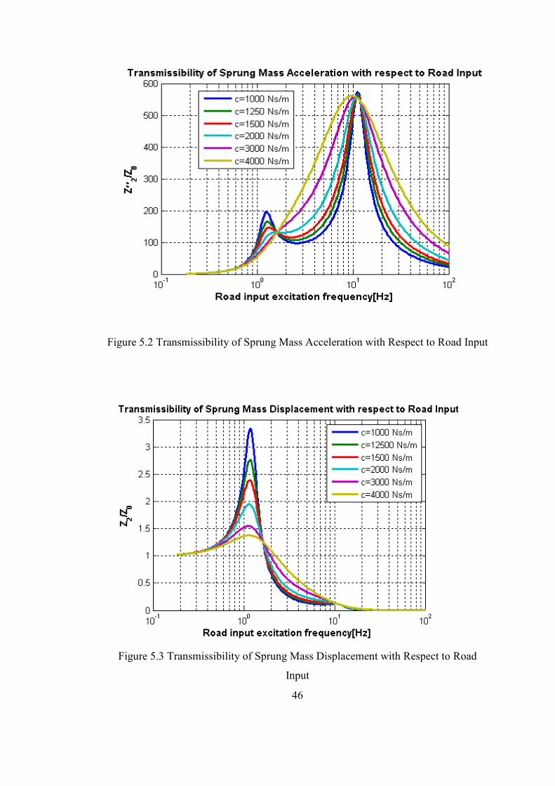
46

Figure 5.2 Transmissibility of Sprung Mass Acceleration with Respect to Road Input

Figure 5.3 Transmissibility of Sprung Mass Displacement with Respect to Road

Input

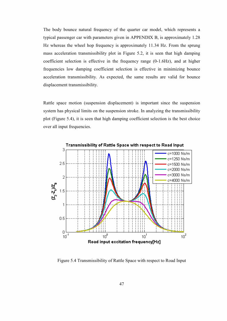
47

The body bounce natural frequency of the quarter car model, which represents a

typical passenger car with parameters given in APPENDIX B, is approximately 1.28

Hz whereas the wheel hop frequency is approximately 11.34 Hz. From the sprung

mass acceleration transmissibility plot in Figure 5.2, it is seen that high damping

coefficient selection is effective in the frequency range (0-1.6Hz), and at higher

frequencies low damping coefficient selection is effective in minimizing bounce

acceleration transmissibility. As expected, the same results are valid for bounce

displacement transmissibility.

Rattle space motion (suspension displacement) is important since the suspension

system has physical limits on the suspension stroke. In analyzing the transmissibility

plot (Figure 5.4), it is seen that high damping coefficient selection is the best choice

over all input frequencies.

Figure 5.4 Transmissibility of Rattle Space with respect to Road Input

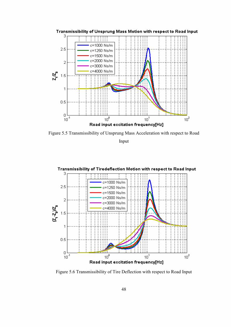
48

Figure 5.5 Transmissibility of Unsprung Mass Acceleration with respect to Road

Input

Figure 5.6 Transmissibility of Tire Deflection with respect to Road Input

49

It is observed that the transmissibility plot of unsprung mass displacement in Figure

5.5 is mainly affected by the damping coefficient of the suspension damper at the

wheel hop natural frequency. The unsprung mass motion together with tire deflection

transmissibility (Figure 5.6) is of concern in relation to vehicle handling rather than

ride comfort. On the other hand, excessive tire deflection may affect the vehicle

performance drastically. As can be seen from both plots, higher damping coefficient

selection is the best choice for isolation at frequencies greater than approximately 5

Hz and frequencies lower than 1.28 Hz. Selection of low damping coefficient proves

to be useful for input frequencies between 1.28 Hz and 5 Hz.

To sum up the results, one can divide the frequency range in 3 sections roughly as:

Region 1 - up to nearby body bounce natural frequency (1.3 Hz)

Region 2 - between body bounce natural frequency and 4.5 Hz

Region 3 - beyond 4.5 Hz

In region 1, minimizing the body bounce motion, sprung mass motion and rattle

space motion all together is only possible by choosing a damper with a high damping

coefficient. In region 2, minimizing body bounce motion and sprung mass motion is

best achieved by choosing a damper with a low damping coefficient. The rattle space

motion in region 2 is not very sensitive to damping coefficient changes, so its

optimization may be omitted to avoid unnecessary complexity.

In region 3, minimizing body bounce motion, sprung mass motion and rattle space

motion simultaneously is not possible. Therefore, a trade-off between these

optimization parameters should be made by the control algorithm designer. The

importance level of these motion transmissibilities defined by the control algorithm

designer, leads the choice between high and low damping coefficients. The main

advantage of the semi-active dampers is their ability to provide low, medium, and

high damping coefficients. It should be kept in mind that if in region 3 sprung mass

acceleration is wanted to be minimized so low damping coefficient will be selected

such that sprung mass and rattle space motion will be adversely affected. In case of

50

optimal control, if only bounce acceleration is chosen to be minimized, the damping

constant is chosen as low as possible in region 3 such that the transmissibilities of

rattle space and unsprung mass motion around wheel hop frequency increase.

Naturally semi-active dampers can be controlled based on the feedback of velocity,

and displacement measurements on vehicle states by supplying necessary current

inputs to them. For minimizing bounce acceleration the semi-active control supplies

maximum feasible current in the frequency regions 1 and 2. In region 3, the semi-

active damper should supply zero current to provide the lowest damping possible like

in the uncontrolled case where no current is supplied. Another drawback of lowering

the damping in region 3 is the tendency of increasing oscillation magnitudes due to

low damping. Although obtaining smaller bounce acceleration peak values, the RMS

values have the affinity to increase.

The optimal dampers attempt to maintain the most convenient damping forces based

on the states of the vehicle. Discussions about transmissibility plots are necessary to

analyze the potentials of a control method. A suitable control law for a quarter car

model can be defined as supplying maximum feasible current in the frequency region

1 and probably in region 2. In region 3, if only bounce acceleration is important, the

semi-active damper should supply null current, in which case the results will be the

same as those of uncontrolled case. Although low damping coefficients are desirable

in the frequency region 3, low damping levels can cause the vehicle to have

oscillations such that the settling time of the system is increased. If one has to

compromise between different optimization parameters in region 3, the damper

current should be regulated accordingly.

As a last statement, the study is carried on a quarter car model; however in the actual

control model the pitch and roll angles are also controlled. The LQR control strategy

will make the compromise between bounce acceleration, roll and pitch angle

minimization. The damper current will take values between maximum and minimum

current inputs possible to accomplish the compromise.

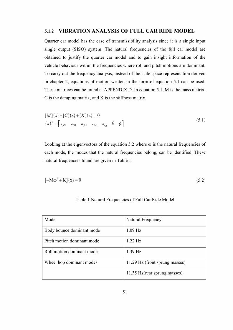
51

5.1.2 VIBRATION ANALYSIS OF FULL CAR RIDE MODEL

Quarter car model has the ease of transmissibility analysis since it is a single input

single output (SISO) system. The natural frequencies of the full car model are

obtained to justify the quarter car model and to gain insight information of the

vehicle behaviour within the frequencies where roll and pitch motions are dominant.

To carry out the frequency analysis, instead of the state space representation derived

in chapter 2, equations of motion written in the form of equation 5.1 can be used.

These matrices can be found at APPENDIX D. In equation 5.1, M is the mass matrix,

C is the damping matrix, and K is the stiffness matrix.

T1 1 1 1

[ ]{ } [ ]{ } [ ]{ } 0

{x}

+ + =

=

ɺɺ ɺ

fl bl fr br cg

M x C x K x

z z z z z θ φ (5.1)

Looking at the eigenvectors of the equation 5.2 where ω is the natural frequencies of

each mode, the modes that the natural frequencies belong, can be identified. These

natural frequencies found are given in Table 1.

2[ Mω K]{x} 0− + = (5.2)

Table 1 Natural Frequencies of Full Car Ride Model

Mode Natural Frequency

Body bounce dominant mode 1.09 Hz

Pitch motion dominant mode 1.22 Hz

Roll motion dominant mode 1.39 Hz

Wheel hop dominant modes 11.29 Hz (front sprung masses)

11.35 Hz(rear sprung masses)

52

5.2 OPTIMIZATION FOR OPTIMAL CONTROL

USING BUMP INPUT

In this section, an optimization process is carried out in order to demonstrate the

design procedure. A half sinusoidal bump with height of 3.5 cm and width of 1 m,

which represent a typical high speed trap, will be used as the input for the

optimization routine. The velocity of the vehicle will be varied from 5 kph to 90 kph

to make the input frequencies dominantly cover the range of 0.7Hz-15Hz. This

frequency range is selected since it covers the body bounce and wheel hop

frequencies and the range of frequencies in which the human body is the most

sensitive. The optimization for optimal control using bump input will be divided into

five stages for deeper analysis of the nature of optimization. In each stage,

optimization is carried out to investigate the best weighing factors at each vehicle

speed, followed by the decision process of a constant weighing factor covering all

velocities. RMS values and peak to peak motion amplitudes are plotted for each case

at every velocity. The stages are namely:

Stage 1: Optimization with respect to only bounce weighting factor

Stage 2: Optimization with respect to only pitch weighting factor

Stage 3: Optimization with respect to bounce acceleration and pitch weighting factor

Stage 4: Optimization with respect to bounce acceleration, pitch, and roll motion

weighting factor

The vehicle data is used in this section is taken from (Zuo & Nayfeh, 2003) .

However to get comparable results between uncontrolled case and passive case in

section 5.2.1, the damping constants used in simulations are modified. The front

damping constant is taken as 964 N.s/m and the rear damping constant is taken as

876 N.s/m. MR damper characteristic used is given at APPENDIX E.

53

5.2.1 STAGE 1: OPTIMIZATION WITH RESPECT TO ONLY

BOUNCE WEIGHTING FACTOR

At this stage, different bounce acceleration weighting factors are used for each

vehicle velocity in the range of 5-90 km/h which corresponds approximately the

frequency range of 0.7-15 Hz. In an iterative manner different bounce acceleration

weighting factors ( 1ρ ) are substituted for different vehicle velocities whereas

2 3 4ρ 0, ρ 0,andρ 1= = = . Then the outputs of the system are sorted with respect to

RMS values of the power of the bounce acceleration, the best factors that brings the

bounce acceleration RMS values to a minimum for each velocity are obtained. A

constant weighting factor is chosen in a way the system outputs do not differ highly

from minimal outputs. In figures, the weighting factors are plotted. In Figure 5.7, the

selected weighting factors are marked on the resulting plot. In Figure 5.8 and Figure

5.9, the RMS and peak to peak body bounce acceleration values for uncontrolled and

controlled cases of semi-active suspensions and also for the passive suspensions are

plotted. In the charts of Figure 5.8 and Figure 5.9, the time span used for calculating

the RMS values is between the time the front wheels encounter the road input and the

time the rear wheels encounter the road input. This time span is selected to focus on

the bounce motion rather than on both pitch and bounce motions.

It is seen from Figure 5.7 and Figure 5.8 that the constant weighting factor selection

does not affect the RMS values of bounce acceleration or peak-to-peak acceleration

values. The improvement in outputs of the car model for semi-active suspensions to

passive systems can be seen from the plots. Another important remark is that the

control strategy is effective at low velocities which mean low road frequency inputs.

The improvement is not clear at high frequencies. When investigated, it can also be

seen in the quarter car transmissibility plot in Figure 5.2 that the suspension needs a

higher damping ratio to reduce bounce acceleration transmissibility whereas it needs

lowest damping ratio at high frequencies. For high frequency regions, the lowest

damping coefficient means the uncontrolled case.

54

Figure 5.7 Weighting Constants for Sinusoidal Bump Body Bounce Acceleration

Optimization

Figure 5.8 Bump Simulation Results (RMS Body Bounce Acceleration)

5,0E+06

1,0E+07

1,0E+07

1,0E+07

1,0E+10

5,0E+06

1,0E+08 1,0E+07

1,0E+071,0E+07

1,0E+051,0E+08

5,0E+05

0,00

0,20

0,40

0,60

0,80

1,00

1,20

1,40

1,60

1,80

0 20 40 60 80 100

RM

S B

ou

nce

Acc

ele

rati

on

(m

/s2)

Velocity(kph)

Sinusoidal Bump Simulation

semiactive constant

weighting factor 10^7

semiactive best

weihting factors

0,00

0,20

0,40

0,60

0,80

1,00

1,20

1,40

1,60

1,80

0 20 40 60 80 100

RM

S(b

ou

nce

acc

ele

rati

on

m/s

2)

Velocity(kph)


semiactive_constant

passive

uncontrolled

semiactive_best

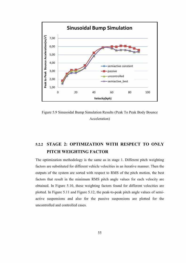
55

Figure 5.9 Sinusoidal Bump Simulation Results (Peak To Peak Body Bounce

Acceleration)

5.2.2 STAGE 2: OPTIMIZATION WITH RESPECT TO ONLY

PITCH WEIGHTING FACTOR

The optimization methodology is the same as in stage 1. Different pitch weighting

factors are substituted for different vehicle velocities in an iterative manner. Then the

outputs of the system are sorted with respect to RMS of the pitch motion, the best

factors that result in the minimum RMS pitch angle values for each velocity are

obtained. In Figure 5.10, these weighting factors found for different velocities are

plotted. In Figure 5.11 and Figure 5.12, the peak-to-peak pitch angle values of semi-

active suspensions and also for the passive suspensions are plotted for the

uncontrolled and controlled cases.

1,00

2,00

3,00

4,00

5,00

6,00

7,00

0 20 40 60 80 100

Pe

ak

to

Pe

ak

B

ou

nce

Acc

ele

rati

on

(m/s

2)

Velocity(kph)


semiactive constant

passive

uncontrolled

semiactive_best

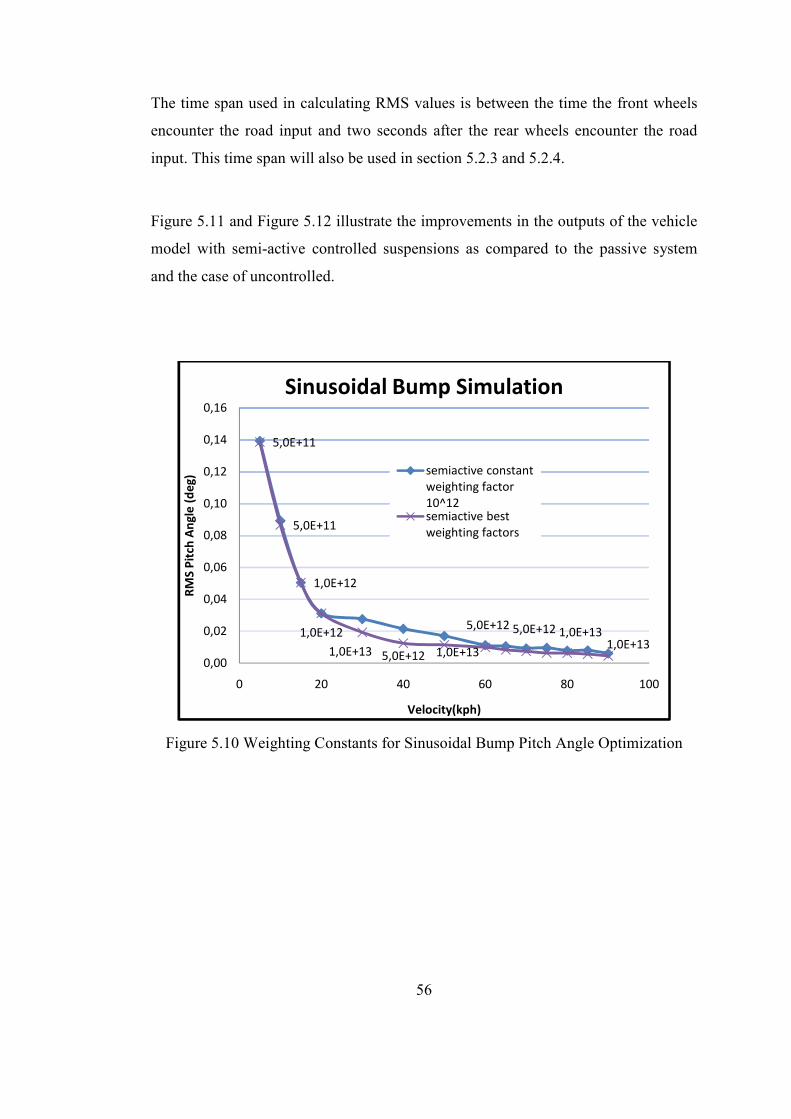
56

The time span used in calculating RMS values is between the time the front wheels

encounter the road input and two seconds after the rear wheels encounter the road

input. This time span will also be used in section 5.2.3 and 5.2.4.

Figure 5.11 and Figure 5.12 illustrate the improvements in the outputs of the vehicle

model with semi-active controlled suspensions as compared to the passive system

and the case of uncontrolled.

Figure 5.10 Weighting Constants for Sinusoidal Bump Pitch Angle Optimization

5,0E+11

5,0E+11

1,0E+12

1,0E+12

1,0E+13 5,0E+12 1,0E+13

5,0E+12 5,0E+12 1,0E+131,0E+13

0,00

0,02

0,04

0,06

0,08

0,10

0,12

0,14

0,16

0 20 40 60 80 100

RM

S P

itch

An

gle

(d

eg

)

Velocity(kph)


semiactive constant

weighting factor

10^12semiactive best

weighting factors

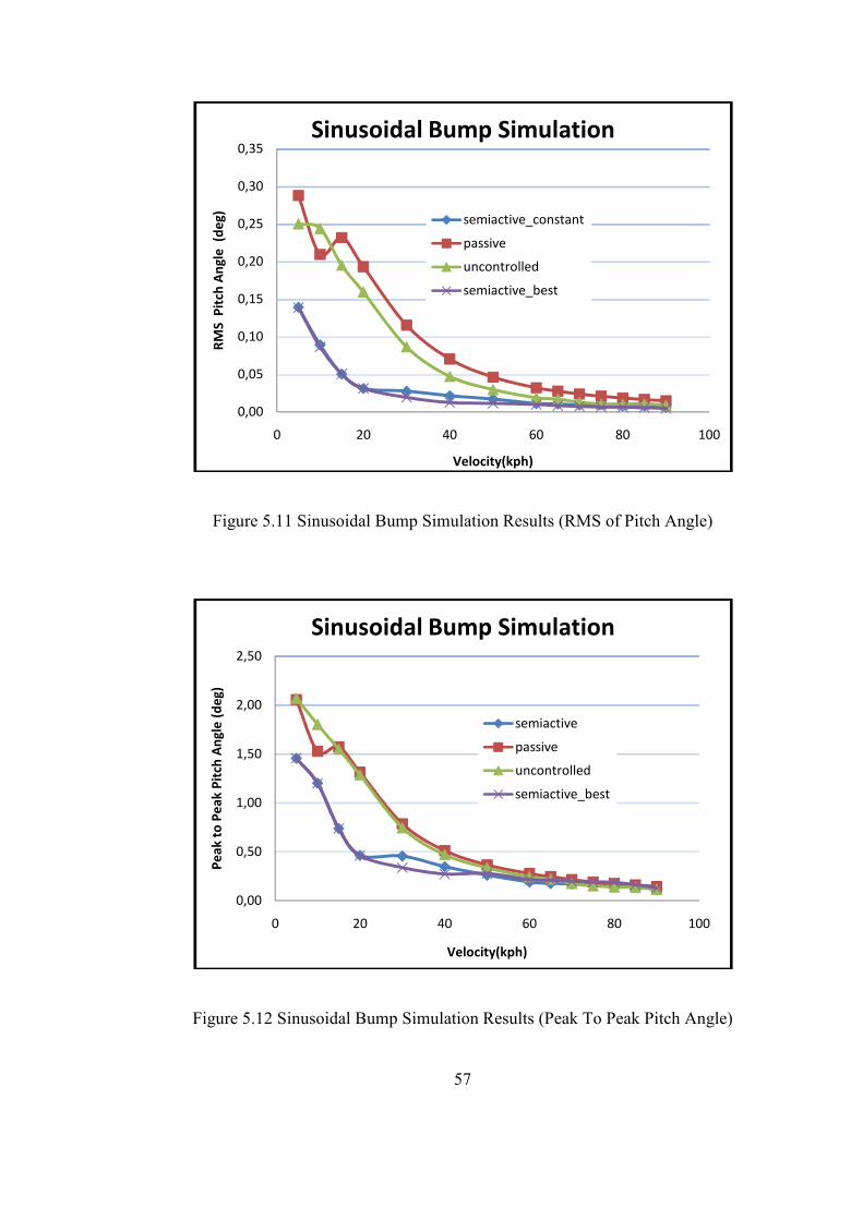
57

Figure 5.11 Sinusoidal Bump Simulation Results (RMS of Pitch Angle)

Figure 5.12 Sinusoidal Bump Simulation Results (Peak To Peak Pitch Angle)

0,00

0,05

0,10

0,15

0,20

0,25

0,30

0,35

0 20 40 60 80 100

RM

S P

itch

An

gle

(d

eg

)

Velocity(kph)


semiactive_constant

passive

uncontrolled

semiactive_best

0,00

0,50

1,00

1,50

2,00

2,50

0 20 40 60 80 100

Pe

ak

to

Pe

ak

Pit

ch A

ng

le (

de

g)

Velocity(kph)


semiactive

passive

uncontrolled

semiactive_best

58

5.2.3 STAGE 3: OPTIMIZATION WITH RESPECT TO BOUNCE

ACCELERATION FACTOR AND PITCH WEIGHTING

FACTOR

In this section, optimization to minimize both bounce acceleration and pitch angle

are studied. In this section, optimization to minimize both bounce acceleration and

pitch angle is 2D optimization which deals with two independent weighting factors.

This procedure will be named as 2D bump optimization. Since the number of states

to be minimized is increased, the complexity of optimization is also increased.

For the optimization process, the array of the bounce acceleration weighting factors

is taken as:

6 6 7 7 8 8 9 9 10 10 1 11

1 110 ,5 10 ,10 ,5 10 10 5 10 10 5 10 10 ,5 10 ,10ρ [ , , , , , 10 ],5⋅ ⋅ ⋅ ⋅ ⋅= ⋅

The pitch angle weighting factor arrays is given as:

8 9 9 10 10 11 11 12

2 125 10 10 5 10 10 ,5 10 ,10 ,5 10 ,10 ,5 1ρ , , , 0[ ]⋅ ⋅ ⋅ ⋅= ⋅

and the roll angle and the control input weighting factors are respectively:

3 4ρ 0, ρ 1= =

The set of velocities considered during the optimization is:

[5,10,15, 20,30, 40,50,60,65,70,75,80,85k h ]p ,90=

In Table 2, the weighting constants to obtain minimum RMS values for bounce

acceleration and pitch angle are listed for different vehicle speeds. Case A refers to

the minimization of RMS values of bounce acceleration, whereas Case B refers to

the minimization of RMS values of pitch angle. As seen from Table 2 , when bounce

acceleration is desired to be minimized, ρ2 takes lower values; whereas ρ1 takes

lower values for the pitch angle minimization.

As a comparison, the minimal values that can be attained by one parameter

optimization in 5.2.1 and 5.2.2 are examined in Figure 5.13 and Figure 5.14. The

59

time span used in calculating RMS values is between the time the front wheels

encounter the road input and two seconds after the rear wheels encounter the road

input. As can be seen from Figure 5.13, the two weighting factor optimization is

better than only bounce acceleration minimization. However, as it can be observed in

Figure 5.14 that there are no distinct performances differences in pitch angle

minimization

Table 2 Weighting Constants for 2D Optimization

Case A: 2D Optimization of RMS Bounce Acceleration Values

Case B: 2D Optimization of RMS Pitch Angle Values

Vehicle CASE A CASE B

Speed ρ1 ρ2 ρ1 ρ2

5 5.E+08 1.E+11 5.E+06 5.E+11

10 5.E+06 1.E+10 5.E+06 5.E+11

15 1.E+07 1.E+10 5.E+06 1.E+12

20 1.E+07 5.E+09 1.E+06 5.E+12

30 5.E+06 1.E+09 1.E+07 5.E+12

40 5.E+10 5.E+10 1.E+08 5.E+12

50 5.E+09 5.E+08 1.E+08 5.E+12

60 1.E+11 5.E+11 1.E+11 5.E+12

65 1.E+07 5.E+10 5.E+08 5.E+12

70 5.E+09 1.E+11 1.E+07 5.E+12

75 1.E+07 5.E+08 1.E+06 5.E+12

80 5.E+06 5.E+09 5.E+07 1.E+12

85 5.E+10 5.E+10 5.E+06 5.E+11

90 1.E+06 5.E+08 5.E+07 1.E+12

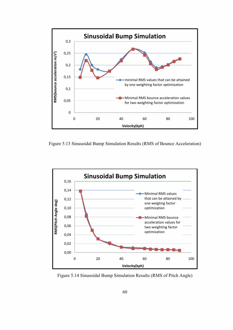
60

Figure 5.13 Sinusoidal Bump Simulation Results (RMS of Bounce Acceleration)


0

0,05

0,1

0,15

0,2

0,25

0,3

0 20 40 60 80 100

RM

S(b

ou

nce

acc

ele

rati

on

m/s

2)

Velocity(kph)


minimal RMS values that can be attained

by one weighting factor optimization

Minimal RMS bounce acceleration values

for two weighting factor optimization

0,00

0,02

0,04

0,06

0,08

0,10

0,12

0,14

0,16

0 20 40 60 80 100

RM

S(P

itch

An

gle

de

g)

Velocity(kph)


Minimal RMS values

that can be attained by

one weigting factor

optimization

Minimal RMS bounce

acceleration values for

two weighting factor

optimization

61

In this particular optimization procedure 1512 optimizations are carried, there should

be some predefined criteria in sorting the results of the optimizations. In the previous

study, with only one weighting factor optimization, it was seen that the bounce

acceleration and pitch angle differences between controlled and uncontrolled results

decrease as the vehicle velocity is increased. So the control effort is focused on low

velocity optimization. This analysis was carried out for 0 to 70 kph. A performance

criterion should be defined to measure the performance improvement in bounce

acceleration and pitch angle at each vehicle velocity:

cg cg

1

cg

z (uncontrolled) z (controlled)P

z (uncontrolled)

−=ɺɺ ɺɺ

ɺɺ (5.3)

2

(uncontrolled) (controlled)P

(uncontrolled)

φ −φ=

φ (5.4)

In this index RMS values of bounce acceleration and pitch angle are used. The time

to calculate RMS values is selected as two seconds after the bump enters the back

wheels. This time is far adequate to damp the oscillations. The indices are unitless

which make them easier to work with.

The following methodology is proposed for determining the optimum constant

weighting factors. P1 and P2 defined in equations 5.3 and 5.4 are found for each

weighting constant set and for different vehicle speeds. The weighting constants

which make P1 or P2 negative are removed from the list, so any controlled response

worse than uncontrolled responses is eliminated. Average P1 for each velocity is

calculated by calculating the average of the P1 values of the reduced list which only

contains superior performance than uncontrolled results. If bounce RMS

minimization is set as the first priority, the weighting constant sets for each velocity

that make P1 better than average P1 values should be emphasized. So by this

manipulation the new list is further reduced to weighting factor sets that minimize

the bounce acceleration more than average performance improvements at a specific

velocity. Analyzing the reduced list further, suitable factors at different vehicle

62

speeds are examined and the set of most frequently appearing weighting factors.

There can be several alternative solutions with which one can select good P1 and P2

indices. By this methodology, a suitable set for all vehicle speeds is chosen as

6 101 2ρ 5 10 ρ 10= ⋅ = among several alternatives. The effect of this methodology to

RMS values of bounce acceleration and pitch angle will be compared to minimal

values that can be attained by two parameter optimization at each velocity

In Figure 5.15 and Figure 5.16 constant weighting factor optimization for 1D and 2D

for all velocities, are also compared to passive and uncontrolled cases. As stated in

the beginning of section 5.2.3, 2D optimization corresponds to bounce acceleration

and pitch angle weighting factor optimization. 1D bump optimization corresponds to

optimization of only bounce acceleration factor or only pitch angle weighting factor.

1D constant parameter optimization constants were evaluated in sections 5.2.1 and

5.2.2.

As can be seen from Figure 5.15 and Figure 5.16 constant weighting factor

optimization for 2D cases is better in performance than other cases at low velocities.

The performance improvement is not so clear at velocities higher than 40 kph. This

result was expected because high frequency inputs as discussed in 5.1.1 needs

minimum damping which corresponds to uncontrolled case.

As can be seen from Figure 5.16, constant weighting factor optimization for 2D cases

is worse in performance than 1D case optimization. The reason is that the

methodology sets priority on minimization of bounce acceleration values. Both 1D

and 2D optimizations are better in performance than the uncontrolled cases.

63

Figure 5.15 Sinusoidal Bump Simulation Results (RMS of Bounce Acceleration)


0,00

0,05

0,10

0,15

0,20

0,25

0,30

0,35

0,40

0,45

0,50

0 20 40 60 80 100

RM

S B

bo

un

ce A

cce

lera

tio

n (

m/s

2)

Velocity(kph)


semiactive_constant_2D_optimization

passive

uncontrolled

semiactive_constant_1D_optimization

0,00

0,05

0,10

0,15

0,20

0,25

0,30

0,35

0,40

0 20 40 60 80 100

RM

S P

itch

An

gle

(d

eg

)

Velocity(kph)


semiactive_constant_2

D_optimization

passive

uncontrolled

constant_semiactive_1

D_optimization

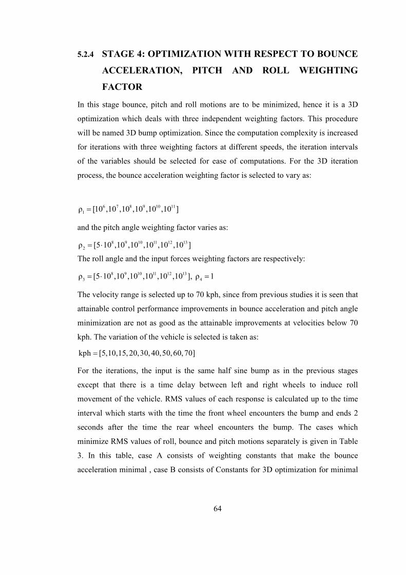
64

5.2.4 STAGE 4: OPTIMIZATION WITH RESPECT TO BOUNCE

ACCELERATION, PITCH AND ROLL WEIGHTING

FACTOR

In this stage bounce, pitch and roll motions are to be minimized, hence it is a 3D

optimization which deals with three independent weighting factors. This procedure

will be named 3D bump optimization. Since the computation complexity is increased

for iterations with three weighting factors at different speeds, the iteration intervals

of the variables should be selected for ease of computations. For the 3D iteration

process, the bounce acceleration weighting factor is selected to vary as:

6 7 8 9 101

11ρ [ , ,10 ,10 10 10 10 ,10, ]=

and the pitch angle weighting factor varies as:

8 9 10 11 12 12

35 10 10 10 ,1ρ [ , 0 ,10 ,10 ],= ⋅

The roll angle and the input forces weighting factors are respectively:

8 9 1 13 4

0 11 12 35 10 10 10 ,10 ,10 ,1ρ [ 10, , ], ρ⋅= =

The velocity range is selected up to 70 kph, since from previous studies it is seen that

attainable control performance improvements in bounce acceleration and pitch angle

minimization are not as good as the attainable improvements at velocities below 70

kph. The variation of the vehicle is selected is taken as:

[5,10,15, 20,30, 40,50,60kph , 70]=

For the iterations, the input is the same half sine bump as in the previous stages

except that there is a time delay between left and right wheels to induce roll

movement of the vehicle. RMS values of each response is calculated up to the time

interval which starts with the time the front wheel encounters the bump and ends 2

seconds after the time the rear wheel encounters the bump. The cases which

minimize RMS values of roll, bounce and pitch motions separately is given in Table

3. In this table, case A consists of weighting constants that make the bounce

acceleration minimal , case B consists of Constants for 3D optimization for minimal

65

pitch angles whereas case C consists of Constants for 3D optimization for minimal

roll angles.

Table 3 Weighting Constants for 3D Bump Optimization

Case A: 3D Optimization for Minimal RMS Bounce Acceleration Values

Case B: 3D Optimization for Minimal RMS Pitch Angle Values

Case C: 3D Optimization or Minimal RMS Roll Angle Values

Vehicle CASE A CASE B CASE C

ρ1 ρ2 ρ3 ρ1 ρ2 ρ3 ρ1 ρ2 ρ3

Speed

5 1.E+06 1.E+11 1.E+11 1.E+06 1.E+12 1.E+11 1.E+06 5.E+08 1.E+12

10 1.E+08 1.E+10 1.E+09 1.E+06 1.E+12 1.E+11 1.E+06 1.E+09 1.E+12

15 1.E+10 1.E+10 1.E+09 1.E+08 1.E+12 5.E+08 1.E+08 1.E+09 1.E+12

20 1.E+10 1.E+10 1.E+11 1.E+07 1.E+12 5.E+08 1.E+08 1.E+10 1.E+12

30 1.E+08 1.E+10 1.E+11 1.E+08 1.E+12 1.E+09 1.E+11 1.E+09 1.E+12

40 1.E+10 1.E+11 1.E+10 1.E+07 1.E+12 1.E+12 1.E+06 1.E+11 5.E+08

50 1.E+06 1.E+11 5.E+08 1.E+07 1.E+12 1.E+11 1.E+11 1.E+11 1.E+11

60 1.E+06 1.E+11 1.E+11 1.E+06 1.E+12 1.E+12 1.E+09 1.E+12 1.E+11

70 1.E+06 1.E+12 1.E+09 1.E+09 1.E+12 1.E+09 1.E+11 1.E+12 1.E+11

The following methodology which was proposed in 5.2.3 is now extended for 3D

optimization. P1, P2 and P3 which are defined in equation (5.5), (5.6) and (5.7) are

found for each weighting constant set and for different vehicle speeds. The weighting

constants which makes P1, P2, or P3 negative is removed from the list, so any

controlled response worse than uncontrolled responses is eliminated. Average P1 for

each velocity is calculated by calculating the average of the P1 values of the reduced

list which only contains superior performance achievements than uncontrolled

results. If bounce RMS minimization is set as the first priority, the weighting

constant sets that make P1 better than average P1 values should be emphasized. So by

66

this manipulation the new list is further reduced to weighting factor sets that

minimize the bounce acceleration more than average at a specific velocity. The list

can be further reduced by applying same procedure for P2 and P3. However this type

of overall reduction for P1, P2, and P3. was not feasible in finding the most frequently

appearing weighting factor sets for every vehicle speed, since a suitable weighting

factor set could not be found after the overall reduction in the list. So the procedure is

only carried for P1 and P3. The emphasis is given to minimization of bounce

acceleration and roll angle. Analyzing the reduced list, the suitable factors at

different vehicle speeds are examined and are found. There can be several alternative

solutions which one can select with good P1 and P3 indices. By this methodology, a

suitable set for all vehicle speeds is chosen as 6 10 101 2 2ρ 5 10 ρ 10 ρ 10= ⋅ = = among

several alternatives.

cg cg

1

cg

z (uncontrolled) z (controlled)P

z (uncontrolled)

−=ɺɺ ɺɺ

ɺɺ (5.5)

2

(uncontrolled) (controlled)P

(uncontrolled)

φ −φ=

φ (5.6)

3

θ(uncontrolled) θ(controlled)P

θ(uncontrolled)

−=

(5.7)

The effect of this methodology for RMS values of bounce acceleration is given in

Figure 5.17 . As can be seen there is a performance improvement of the control

strategy between uncontrolled and controlled results. By using semi-active constant

factors there is a slight performance decrease from optimal ones, the performance

increase is better from uncontrolled and controlled results. The plots for roll angle

and pitch angle RMS values are given in Figure 5.18 and Figure 5.19.

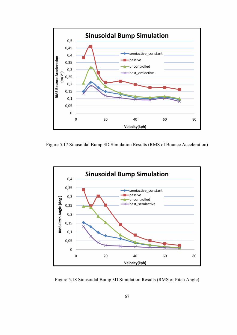
67

Figure 5.17 Sinusoidal Bump 3D Simulation Results (RMS of Bounce Acceleration)

Figure 5.18 Sinusoidal Bump 3D Simulation Results (RMS of Pitch Angle)

0

0,05

0,1

0,15

0,2

0,25

0,3

0,35

0,4

0,45

0,5

0 20 40 60 80

RM

S B

ou

nce

Acc

ele

rati

on

(m/s

2)

Velocity(kph)


semiactive_constant

passive

uncontrolled

best_emiactive

0

0,05

0,1

0,15

0,2

0,25

0,3

0,35

0,4

0 20 40 60 80

RM

S P

itch

An

gle

(d

eg

)

Velocity(kph)


semiactive_constant

passive

uncontrolled

best_semiactive

68

Figure 5.19 Sinusoidal Bump 3D Simulation Results (RMS of Roll Angle)

5.3 3D BUMP OPTIMIZATION FOR SKYHOOK

CONTROL STRATEGIES

Skyhook control strategy for semi-active suspension control is widely used. So for

comparison purposes with the optimal control approach used in this study, a

reference skyhook controller will be developed and tested. The same optimization

process described in section 5.2 should be done to find front and rear skyhook

damping constants for skyhook control algorithm. Since the vehicle is symmetric

about the roll axis, the optimization process is carried for front and rear skyhook

constants. Also since the centre of gravity is close to the front side, the front damping

constant is expected to be selected higher than or equal to the rear damping

constants. The possible skyhook gains are selected as [1500 2500 3000 3500 4000

4500 5000 5500 6000 7000 8000 9000]. Some sample trials lead to a range of

0

0,02

0,04

0,06

0,08

0,1

0,12

0 20 40 60 80

RM

S R

oll

An

gle

(De

g)

Velocity(kph)


semiactive_constant

passive

uncontrolled

best_semaictive

69

skyhook damping values between 2500 and 6000. Hence the damping range between

these constants is divided more finely than the entire range. The velocity variations

are selected same as the section 5.2 and taken as [5 10 15 20 30 40 50 60 70] kph.

The optimization procedure is done to minimize the bounce acceleration, pitch angle,

and roll angle as was done in section 5.2. Suitable performance criterion for P1, P2,

and P3 are evaluated for different vehicle speeds going on the same bump. The 3D

optimization strategy for skyhook control procedure is easier to handle since only

two damping constants are to be found whereas in 3D optimization three weighting

factors were determined. The same methodology in section 5.2.4 is carried for this

optimization. The front damping is selected as 5000Ns/m whereas the rear damping

is selected as 4500 Ns/m. The results from skyhook control will now be compared

with optimal control in section 5.4.

5.4 3D CHIRP INPUT ANALYSIS

When comparative results between different control strategies are needed to verify a

design under general conditions, frequency response techniques are commonly used.

Since the model is nonlinear, the classical approach for obtaining frequency response

cannot be used. For nonlinear systems, hammer inputs and chirp inputs are generally

used to find the frequency response.

The 7-dof vehicle ride model can be excited with a chirp signal to determine its

frequency response. The chirp signal is generated in Matlab Simulink by a chirp

signal block which generates a sine wave whose frequency increases at a linear rate

with time. This simulation enables a frequency domain analysis. Although the chirp

input test cannot be generalized, it gives an idea about the efficiency of the

controller. The fast Fourier transform of the system outputs for a given chirp input

gives an idea of the response of the system for different frequencies. The simulation

input will contain all frequencies between 0.1 Hz to 17 Hz. This frequency range

covers the basic frequency range interest of the ride comfort for passengers. Chirp

input time is selected as 70 seconds. The sine input amplitude is selected as 0.035 m.

70

The inputs to left and right wheels should have a time delay difference to induce roll

motion. The time difference between rear and front wheels is based on the vehicle

speed. The time delay between wheels complicates the frequency response by

dispersing the expected peaks at natural frequencies. This effect can be seen from

Figure 5.20 which represents the bounce motion response when the chirp inputs

applied at the front wheels. The same inputs are assumed to excite the back wheels

with a time delay corresponding to a vehicle speed of 72 kph. Also a time delay of

0.05 seconds is applied to the right wheels with respect to left wheels to create roll

motion.

To overcome the difficulty of four separate inputs, the inputs which have same

characteristics at each wheel should be applied at the same time. There should also

be no delay between the wheels for clarity in frequency response Since the four

inputs of same characteristics are meaningless, the vehicle is assumed to be affected

from only one wheel to get a clear frequency response. This situation is evidently

fictitious; however it gives a measure of the frequency response. Giving input to only

one of the wheels can excite both roll, pitch, and bounce motions. The corresponding

frequency responses are given for this special input in the following figures. In the

legends, “SUBoptimal” is used to represent the clipped optimal law. To the rest of

the chirp input analysis in this section and the simulations in section 6, the vehicle

data (Zuo & Nayfeh, 2003) in APPENDIX B will be used.

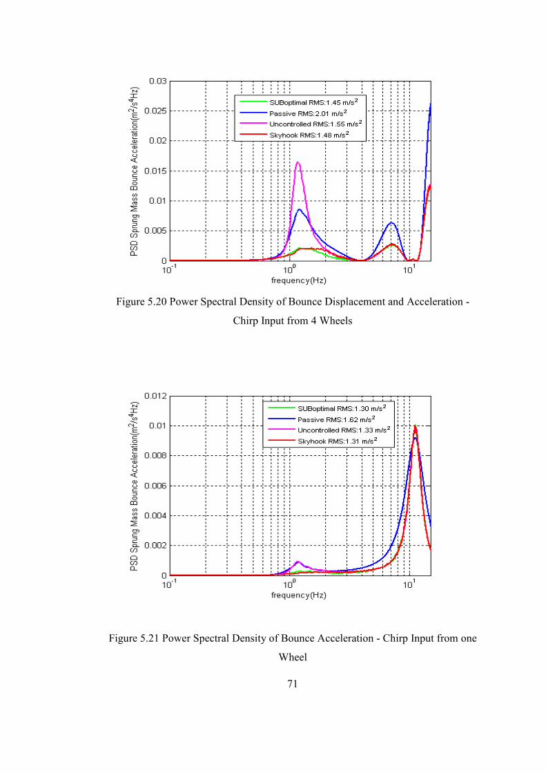
71

Figure 5.20 Power Spectral Density of Bounce Displacement and Acceleration -

Chirp Input from 4 Wheels

Figure 5.21 Power Spectral Density of Bounce Acceleration - Chirp Input from one

Wheel

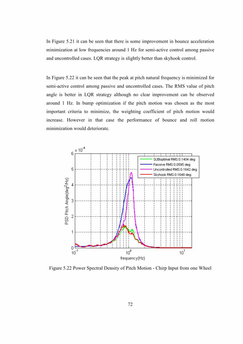
72

In Figure 5.21 it can be seen that there is some improvement in bounce acceleration

minimization at low frequencies around 1 Hz for semi-active control among passive

and uncontrolled cases. LQR strategy is slightly better than skyhook control.

In Figure 5.22 it can be seen that the peak at pitch natural frequency is minimized for

semi-active control among passive and uncontrolled cases. The RMS value of pitch

angle is better in LQR strategy although no clear improvement can be observed

around 1 Hz. In bump optimization if the pitch motion was chosen as the most

important criteria to minimize, the weighting coefficient of pitch motion would

increase. However in that case the performance of bounce and roll motion

minimization would deteriorate.

Figure 5.22 Power Spectral Density of Pitch Motion - Chirp Input from one Wheel

73

In Figure 5.23 it can be seen that there is also an improvement for semi-active

suspensions in roll motion minimization at low frequencies around 1 Hz. The RMS

values for both accelerations and motions are also minimal for semi-active control

among passive and uncontrolled cases. In semi-active controls, the LQR controller

performance is better than skyhook controllers.

As can be seen from Figure 5.24, rattle space movement is minimized at frequencies

around 1 Hz.

Figure 5.23 Power Spectral Density Of Roll Motion - Chirp Input From One Wheel

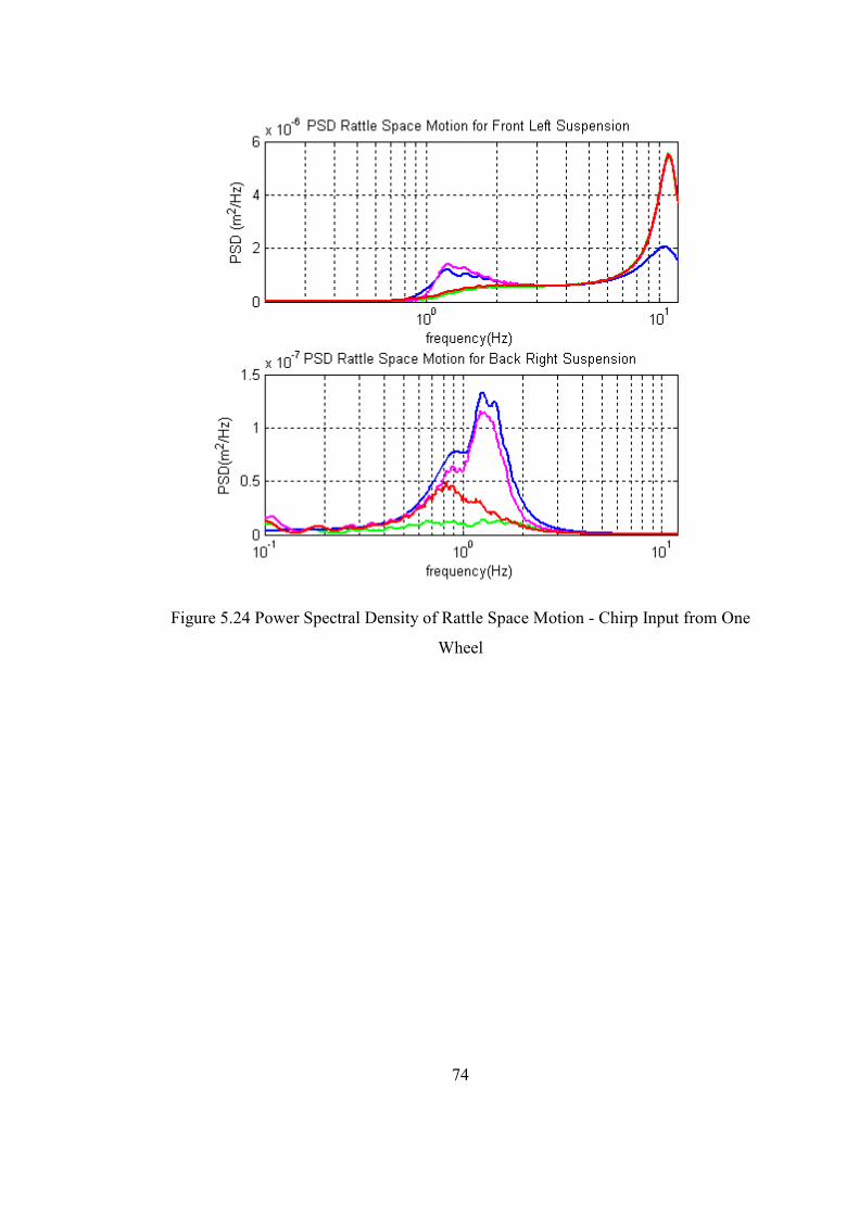
74

Figure 5.24 Power Spectral Density of Rattle Space Motion - Chirp Input from One

Wheel

75

CHAPTER 6

6 SIMULATION TESTS

6.1 SINUOSIDAL INPUT TEST

This input is proposed to examine the response of the vehicle near the natural

frequencies of bounce, pitch, and roll motions. The input is selected as a continuous

1 Hz sinusoidal input with an amplitude of 3.5 cm which corresponds to a width of

0.69 m and a velocity of 5 kph. There is a time delay between front and rear wheels

dependent on the velocity of the car. To induce roll motion the sinusoidal input is

only applied with a time shift of 0.2 radian between left and right sides of the car.

The time responses are plotted in Figure 6.1, Figure 6.2, Figure 6.3, and Figure 6.4.

.The Root Mean Square values (RMS) for each control policy computed in the time

span of 10 seconds can be seen in the legends of the plots.

In Figure 6.1, the bounce displacement is plotted .The transient behaviour is due to

the time delay between front and rear wheels. There is high frequency oscillation

added to 1 Hz oscillations in bounce acceleration due to the limits of semi-active

control for the minimal and maximum damping forces. As can be seen there is a

significant reduction of bounce motion for semi-active control.

In Figure 6.7 and Figure 6.8 the improvements of pitch and roll motions can be seen

respectively.

76

Figure 6.1 Bounce Displacement and Acceleration versus Time – Sinusoidal Input

Figure 6.2 Pitch Angle versus Time - Sinusoidal Input

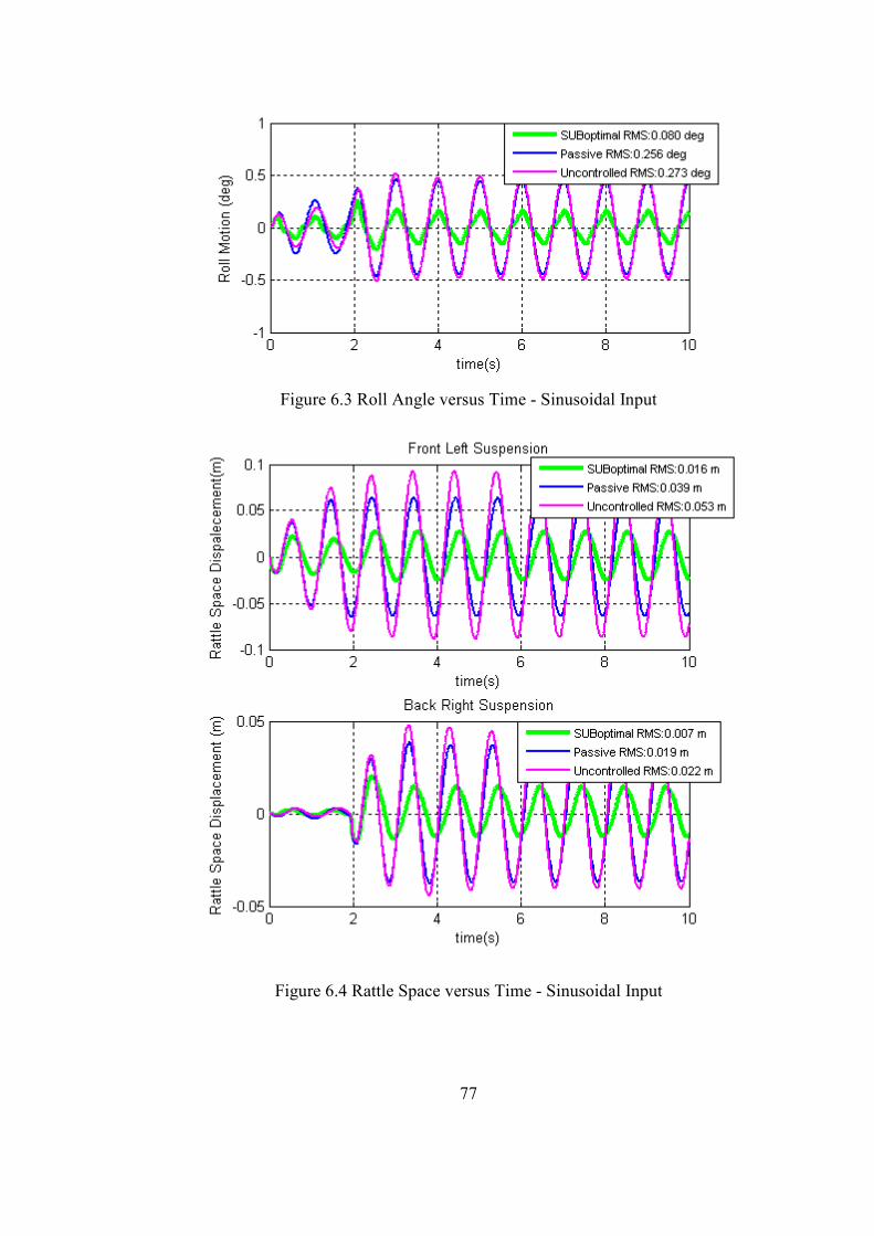
77

Figure 6.3 Roll Angle versus Time - Sinusoidal Input

Figure 6.4 Rattle Space versus Time - Sinusoidal Input

78

6.2 BUMP&HUMP TEST

The inputs will correspond to single bumps or humps that will pass through two

axles or only right or left wheels of the vehicle. The speed of the vehicle is taken as

30-50 kph since the speed limit in city centers where speed control humps is used.

The geometrical information about more commonly used humps can be found from

the document of TS 6283(Turkish Standard Institution, 1998). In this work it is stated

that the length of the half sinusoidal flat humps is between 3.6 m to 3.8 m whereas

the height of the bump is 7.5 to 10 cm.

In case of the half sinusoidal short bumps the width of the bump has the length 30 to

100 cm whereas the height of the bump is between 3 to 10 cm.

6.2.1 HALF SINUSOIDAL BUMP TEST SIMULATION 1

This input is proposed to examine the transient response of the vehicle due to bump

inputs. The input is selected as a half sinusoidal bump with a height of 3.5 cm and

with a width of 1 meter at a velocity of 9 kph. There is a time delay between front

and rear wheels dependent on the velocity of the car. To induce roll motion the

sinusoidal input is only applied to the left side of the car. The input can be also seen

from Figure 6.5. The settling time of three control policies can be identified from the

time response plots in Figure 6.6, Figure 6.7, Figure 6.8, and Figure 6.9. The RMS

values for the time span of 5 seconds are given in the legends of the figures.

79

Figure 6.5 Road Input versus Time - Half Sinusoidal Bump Input Case 1

This type of input excitation is applied to give low frequency road inputs. The

improvements are very clear for settling time, peak to peak value minimization, and

RMS minimization of the system outputs. As was discussed in section 5.1.1 the

improvement of ride comfort and handling is possible for low frequency range as can

also be seen for the cases of this input.

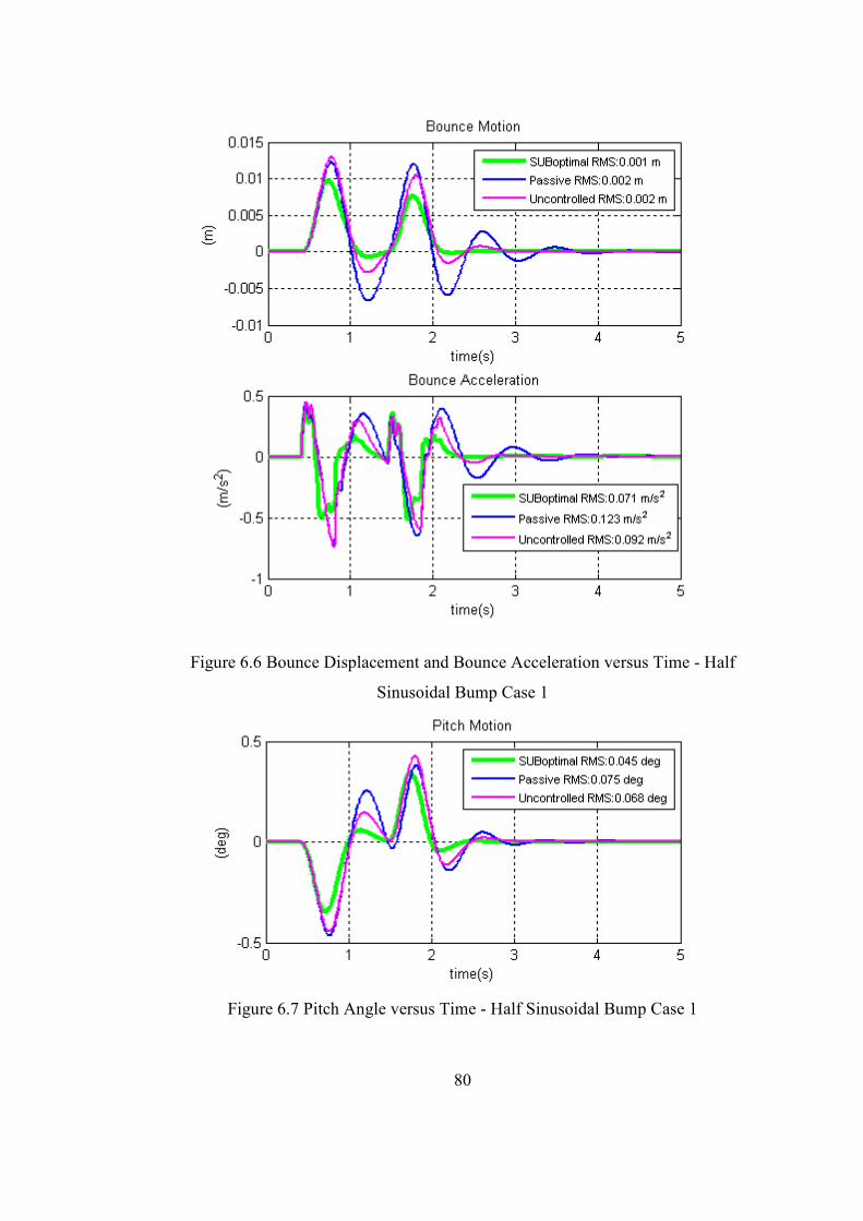
80

Figure 6.6 Bounce Displacement and Bounce Acceleration versus Time - Half

Sinusoidal Bump Case 1

Figure 6.7 Pitch Angle versus Time - Half Sinusoidal Bump Case 1

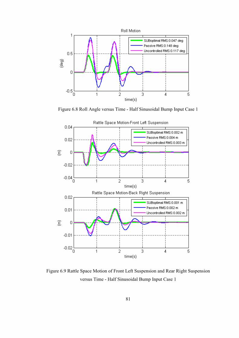
81

Figure 6.8 Roll Angle versus Time - Half Sinusoidal Bump Input Case 1

Figure 6.9 Rattle Space Motion of Front Left Suspension and Rear Right Suspension

versus Time - Half Sinusoidal Bump Input Case 1

82

6.2.2 HALF SINUSOIDAL BUMP TEST SIMULATION 2

The input is selected as a half sinusoidal bump with a height of 7 cm and with a

width of 0.8 m at a velocity of 30 kph. This bump is also used in the work (Choi,

Han, Song, & Choi, 2007). The bump is modified to induce roll motion of the

vehicle. The half sinusoidal input is only applied to the left side of the car. The input

can be also seen from Figure 6.10

The settling time of three control policies can be identified from the time response

plots in Figure 6.11, Figure 6.12, Figure 6.13 and Figure 6.14. The RMS values for

the time span of 5 seconds are given in the legends of the figures.

Figure 6.10 Road Input versus Time - Half Sinusoidal Bump Input Case 2

As can be seen from Figure 6.11 there is an improvement of bounce acceleration

minimization with respect to passive suspensions, however this improvement is not

clear between controlled and uncontrolled cases. The reason is for bounce

acceleration minimization at high frequencies the damping force should be minimal.

The settling time, RMS, and peak to peak values are minimal for semi-active

suspension for bounce, pitch, and roll and rattle space motion.

83


Bump Input Case 2

Figure 6.12 Pitch Motion versus Time - Half Sinusoidal Bump Input Case 2

84

Figure 6.13 Roll Motion versus Time - Half Sinusoidal Bump Input Case 2


Suspension versus Time - Half Sinusoidal Bump Input Case 2

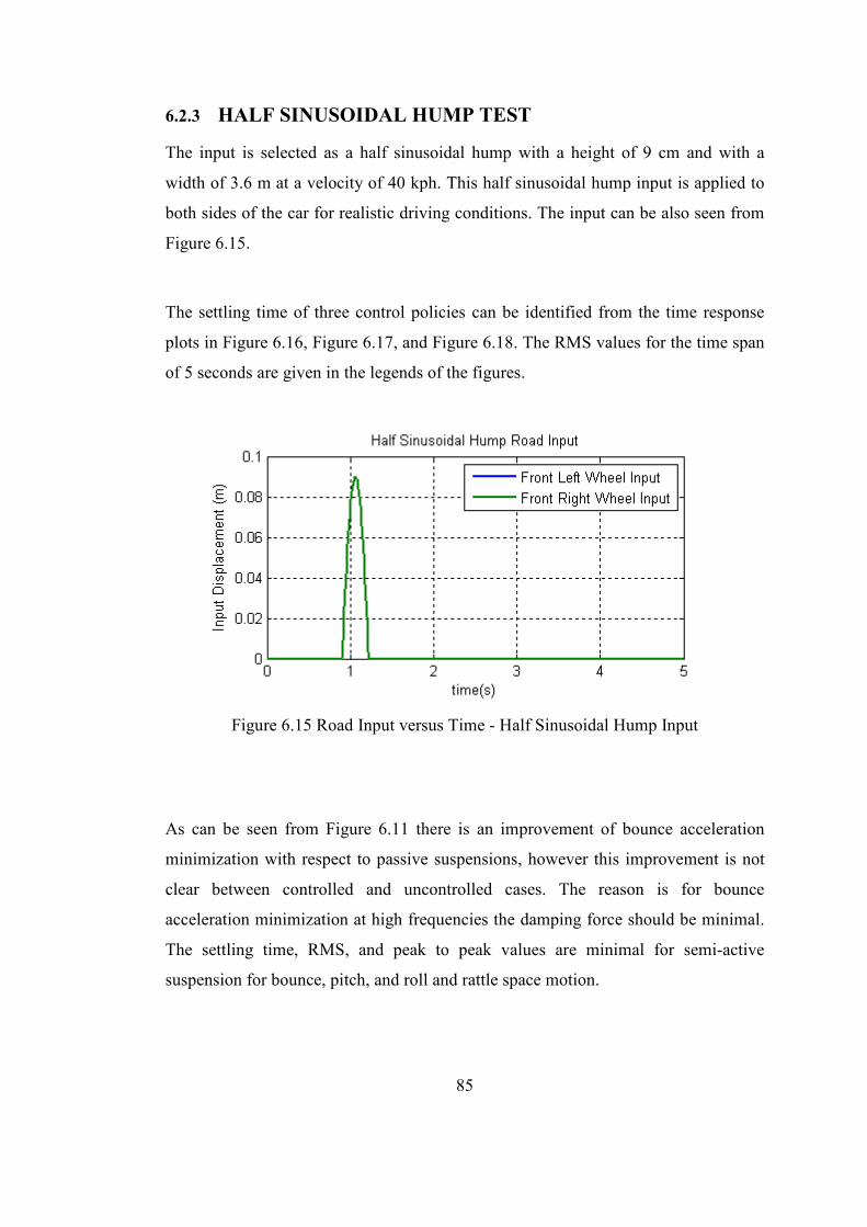
85

6.2.3 HALF SINUSOIDAL HUMP TEST

The input is selected as a half sinusoidal hump with a height of 9 cm and with a

width of 3.6 m at a velocity of 40 kph. This half sinusoidal hump input is applied to

both sides of the car for realistic driving conditions. The input can be also seen from

Figure 6.15.

The settling time of three control policies can be identified from the time response

plots in Figure 6.16, Figure 6.17, and Figure 6.18. The RMS values for the time span

of 5 seconds are given in the legends of the figures.

Figure 6.15 Road Input versus Time - Half Sinusoidal Hump Input

As can be seen from Figure 6.11 there is an improvement of bounce acceleration

minimization with respect to passive suspensions, however this improvement is not

clear between controlled and uncontrolled cases. The reason is for bounce

acceleration minimization at high frequencies the damping force should be minimal.

The settling time, RMS, and peak to peak values are minimal for semi-active

suspension for bounce, pitch, and roll and rattle space motion.

86


Hump Input

Figure 6.17 Pitch Motion versus Time - Half Sinusoidal Hump Input

87


Suspension versus Time - Half Sinusoidal Hump Input

6.3 STEP INPUT TEST

This simulation is carried for determining transient response characteristics. The

settling time can be seen from the plots. The step input height (Figure 6.19) is taken

as 10 cm at a vehicle velocity of 60 kph. For this input the roll motion characteristics

cannot be investigated, since the input does not differ for left and right side of the

vehicle. In Figure 6.20 bounce motion characteristics are plotted whereas in Figure

6.21 and Figure 6.22 pitch angle and rattle space motion is plotted accordingly. As

can be seen from the plots, the settling time for pitch, roll, and bounce motion

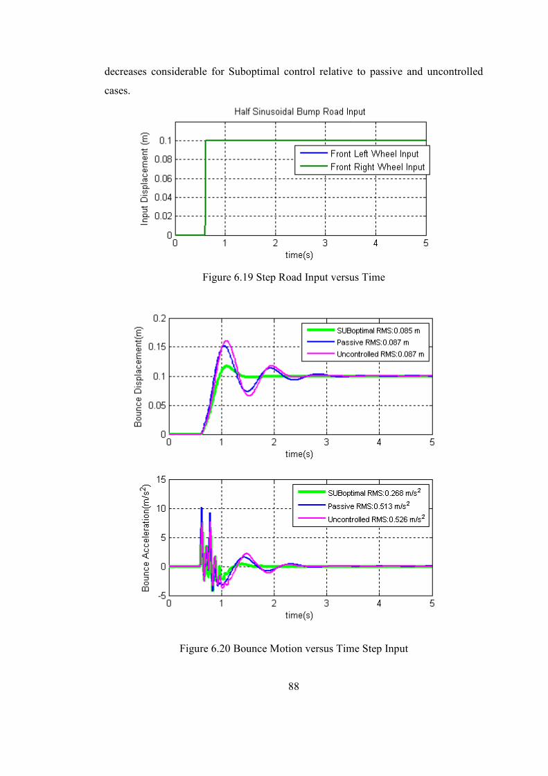
88

decreases considerable for Suboptimal control relative to passive and uncontrolled

cases.

Figure 6.19 Step Road Input versus Time

Figure 6.20 Bounce Motion versus Time Step Input

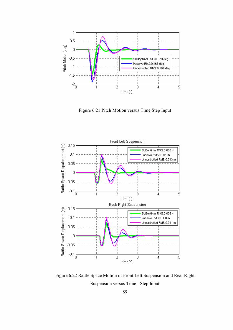
89

Figure 6.21 Pitch Motion versus Time Step Input


Suspension versus Time - Step Input

90

6.4 RANDOM ROAD INPUT TEST

Random road input test is carried with a white noise velocity input to have an idea of

the frequency response of the vehicle. The random road input represents the general

road conditions. The road excitation for a random process with a zero mean

described by the equation:

z ρVz VW+ =ɺ 6.1

where V is the vehicle velocity, z is the road input, W is a white noise of power

spectral intensity of 22σ ρV , 2σ is the variance of road irregularity and ρ is the road

roughness parameter. The road inputs are calculated separately for the left and right

side wheels. The inputs generated for each side of the vehicle are transferred to the

back axle with a time delay depending on the vehicle speed.

For this simulation, the velocity of the vehicle is assumed to be 72 kph, 1ρ 0,45m−=

and 2 2σ 300mm= .In Figure 6.23, the time traces of left and right side road inputs are

plotted.

Figure 6.23 Random Road Input versus Time

91

The performance of the MR damper in minimizing bounce motion is seen in Figure

6.25. The vehicle parameters in APPENDIX B and the MR damper characteristics

are adopted from the work of (Hong, Kim, & Kim, 2007). The relative velocity

values across the damper for a random input is very low and at zero current level

near these relative velocities, the MR damper is stiffer than passive dampers as can

be seen from Figure 6.24. This deteriorates the performance of the controller. The

PSD of the bounce motion shows that the passive damper behaviour becomes

superior at high frequency inputs especially for bounce acceleration minimization.

If theoretically zero current damping forces of MR dampers (uncontrolled Mr

damper characteristic) are reduced to 1/3 of the original damping force characteristic,

the improvement between controlled, uncontrolled, and passive cases become

clearer. The PSD of the fictitious MR damper under random road input is given in

Figure 6.26.

To analyze the RMS values of bounce, pitch and roll motions for MR damper and

fictitious MR damper, a performance criterion is proposed. The performance in

minimizing RMS values is defined by the percentage of the difference between the

obtained value and the passive suspension corresponding RMS value to the passive

suspension RMS value. In the Table 4 the performance improvements are seen for

MR damper. As expected the passive damper is better in bounce motion and pitch

motion minimization, since the damper is stiffer in that region. For the fictitious

damper whose minimum level damping is decreased to one third of the original there

are tangible performance improvements in bounce, pitch and roll motions as shown

in Table 5. As seen, semi-active dampers should be selected in a way that the feasible

damping range should have a broadened damping range which also includes a

suitable passive suspension damping characteristic inside.

92

Figure 6.24 MR and Passive Damper Characteristics


Acceleration of the existing MR damper

93


Acceleration of the fictious MR damper

94

Table 4 Performance Results for the MR Damper under Random Road Input

Performance Improvement of the

Semi-active Control with respect

to Passive Suspension

Performance Improvement of

the Uncontrolled Dampers

with respect to Passive

Suspension

Bounce Motion -50.0% -50.0%

Bounce Acceleration -31.1% -31.3%

Pitch Motion -12.5% -18.8%

Roll Motion 30.6% 6.8%

Table 5 Performance Results for the Fictitious MR Damper under Random Road

Input

Performance Improvement of the

Semi-active Control with respect

to Passive Suspension

Performance Improvement of

the Uncontrolled Dampers

with respect to Passive

Suspension

Bounce Motion 0.0% -25.0%

Bounce Acceleration 16.7% 5.4%

Pitch Motion 17.2% -12.5%

Roll Motion 42.8% -7.3%

95

CHAPTER 7

CONCLUSION

Based on the simulation results, it was seen that semi-active MR dampers are capable

of improving ride comfort by minimizing the bounce, pitch, and roll motion response

with respect to passive dampers and uncontrolled case of semi-active MR dampers.

The settling time and peak responses were reduced. The basic disadvantage of semi-

active control is the worsening of rattle space responses. The increase in rattle space

motion is not significant enough to create problems in suspension stroke limits.

When implementing the semi-active controller, safety measures can be taken in case

of extreme motions of rattle space motion by changing the control strategy.

For today the semi-active damping range for MR dampers is limited. Generally they

are stiff in low relative velocities. This problem affects the random road input

responses adversely. If the semi-active damping range could be broadened, the

results would get better as was shown in section 6.4. The bigger the semi-active

damping range, the more the performance of semi-active controllers improves.

LQR control algorithm is a systematic way to determine how to accomplish a given

task. This strategy can be extended to take into account of the passenger seat motions

and rattle space motion across dampers. The effectiveness of this strategy can be

seen from the simulation results in section 6.1, 6.2, 6.3 and 6.4. The responses

around 1 Hz which is near to body bounce frequency, show the improvement in ride

comfort.

96

Skyhook control is an alternative control strategy which has nearly as significant

improvements as LQR control does. Comparing the performances of skyhook and

LQR control, LQR control is better in minimizing bounce acceleration and roll angle

than skyhook control. The improvement of pitch angle minimization for LQR

controllers is superior to classical passive suspensions; however the performance is

not superior to skyhook controller. This was because more importance was given on

reducing bounce and roll motion in LQR while tuning weighting constants.

The relative performance improvement is comparable to the easiness of

implementation of the skyhook control strategy. LQR control for full car ride model

needs full state feedback of 14 states whereas for skyhook control 8 state feedback is

sufficient. The choice between two control strategies depends on the user

expectations.

As a final remark, the main scope of optimal LQR control can be extended in various

aspects. The LQR controller can be combined with fuzzy controller to compensate

extreme conditions that deviates from normal road inputs. Different weighting factor

sets can be used depending on the vehicle states. The genetic algorithm may be used

in the optimization process of the weighting factors in the LQR controller. Also the

seven degree of freedom model can be extended with additional degree of freedoms

like the driver seat degree of freedom. In addition the cost function index can be

extended to cover rattle space motion. Finally control techniques may be developed

further with Hardware-in-the-Loop (HIL) simulations.

97

REFERENCES

Ahmadian M., S. D. (2004). "Can Semiactive Dampers with Skyhook Control

Improve Roll Stability of Passengers Vehicles?". 2004-01-2099.

Ahmadian, M. P. (2000). A Quarter-Car Experimental Analysis of Alternative Semi

active Control Methods. 11.

Ahmadian, M. S. (2004). No-Jerk Skyhook Control Methods for semiactive

Suspensions. 126.

B.Burl, J. (1999). Linear Optimal Control H2 and Hinfinity Methods. Addison

Wesley.

Butsuen, T. (1989). The Design of Semiactive Suspensions for Automotive Vehicles.

Massachusetts Institute of Technology.

Butz, T. v. (2002). Modeling and Simulation of Electro- and Magnetorheological

Fluid Dampers. 82 (1).

Choi, S. L. (2002). H∞ Control Performance of a Full-Vehicle Suspension Featuring

Magnetorheological Dampers. 38 (5), 341-360.

Choi, S.-B., Han, Y.-M., & Sung, K.-G. (2008). Vibration control of vehicle

suspension. s. 189-204.

Choi, S.-B., Han, Y.-M., Song, H. J., & Choi, H. J. (2007). Field Test on Vibration

Control of Vehicle Suspension System Featuring ER Shock Absorbers. Journal of

Intelligent Material Systems and Structures , 18.

Choi, Y. P. (2000). A Sliding Mode Control of a Full-Car Electrorheological

Suspension System Via Hardware in-the-Loop Simulation. 122.

Dominguez, A. S. (2004). Modeling the Hysteresis Phenomenon of

Magnetorheological Dampers. 13, 1351-1361.

Du, H. S. (2005). Semi-active H∞ Control of Vehicle Suspension with MR Dampers.

283, 981-996.

98

Giua, A. M. (2004). “'Design of a Predictive Semiactive Suspension System. 41 (4),

277-300.

Giua, A. S. (2000). A Mixed Suspension System for a Half-Car Vehicle Model. 10,

375-397.

Giua, A., Seatzu, C., & Usai, G. (1999). Semiactive Suspension Design with an

Optimal Gain Switching Target. Vehicle System Dynamics International Journal of

Vehicle Mechanics and Mobility .

Grad, P. (2006, December). Against the flow - Smart fluids that can change their

viscosity in real time. Engineering & Technology , 1 (9), s. 34-37.

Guglielmino, E. S. (2008). Semi-active Suspension Control - Improved Vehicle Ride

and Road Friendliness . Springer.

Hong, K.-S., Kim, T.-S., & Kim, R.-K. (2007). Sensitivity Control of a Semi-Active

Suspension System Equipped with MR-Dampers. International Conference on

Control, Automation and Systems. Seoul, Korea: IEEE Xplore.

Hong, K.-S., Kim, T.-S., & Kim, R.-K. (2007). Sensitivity Control of a Semi-Active

Suspension System Equipped with MR-Dampers. International Conference on

Control, Automation and Systems 2007. COEX, Seoul, Korea.

Karkoub, M. Z. (2006). Active/semi-active suspension control using

magnetorheological actuators. 37 (1), 35-44.

Kim, R. H. (2007). Skyhook Control Using a Full-Vehicle Model and Four Relative

Displacement Sensors.

Klingenberg, D. J. (2001). Magnetorheology:Applications and Challenges. Aiche

Journal , 17 No:2 249, 246-249.

Li, R. C. (2004). Fuzzy Intelligent Control of Automotive Vibration via Magneto-

rheological Damper. 1-3.

Liu, Y. M. (2004). Controllable Vibration of the Car-Body Using

Magnetorheological Fluid Damper. 41, 627-636.

Lu, J. (2004). A Frequency-Adaptive Multi-Objective Suspension Control Strategy,.

126.

99

Mark R. Jolly, M. R. (1999). Properties and Applications of Commercial

Magnetorheological Fluids.

Martynowicz, P. S. (2007). Experimental Study of Vibration Control in a two Degree

of Freedom Pitch-Plane Model of a Magnetorheological Vehicle Suspension. 26 (2).

Matlab R2007b -The Language of Technical Computing. (n.d.). LQR. Control

System Toolbox .

MR Fluid Techology. (n.d.). Retrieved 01. 07, 2009, from LORD Corporation-

Adhesives, Coatings, Vibration, Shock & Motion Control:

http://www.lord.com/Home/MagnetoRheologicalMRFluid/MRFluidTechnology/Wh

atisMR/tabid/3772/Default.aspx

(n.d.). Retrieved 01 07, 2009, from LORD Corporation – Adhesives, Coatings,

Vibration, Shock & Motion Control.: www.lord.com

Naidu, D. S. (2003). Optimal Control Systems. CRC PRESS.

Ogata, K. Modern Control Engineering-Fourth Edition. Upper Saddle River,New

Jersey: Prentice Hall.

Primary Suspension. (2008). Retrieved 05 08, 2008, from LORD Corporation –

Adhesives, Coatings, Vibration, Shock & Motion Control:

http://www.lord.com/Home/MagnetoRheologicalMRFluid/Applications/PrimarySus

pension/tabid/3329/Default.aspx

Rajamani, R. (2006). Vehicle Dynamics and Control. Springer.

Sinha, A. (2007). Linear Systems Optimal and Robust Control. CRC Press.

Song, X. A. (2005). Modeling Magnetorheological Dampers with Application of

Nonparametric Approach. 16.

Sung, K. C. (2005). Performance Comparison of Mr Dampers with Three Different

Working Modes: Shear, Flow and Mixed Mode. 19 (7,8,9), 1556-1562.

Sung, K.-G., Han, Y.-M., Cho, J.-W., & Choi, S.-B. (2008). Vibration control of

vehicle ER suspension system using fuzzy moving sliding mode controller. Journal

of Sound and Vibration , 1004-1019.

Technology Compared. (n.d.). Retrieved 01 07, 2009, from Lord Corporation-

Adhesives,Coatings,Vibration,and Shock& Motion Control:

100

http://www.lord.com/Home/MagnetoRheologicalMRFluid/MRFluidTechnology/Tec

hnologyCompared/tabid/3773/Default.aspx

Tsang, H. S. (2006). “Simplified inverse dynamics models for MR fluid dampers. 28,

327-341.

Turkish Standard Institution. (1998). Speed Control Humps. Turkish Standard, TS

6283/T3 .

Wang, H. H. (2005). Optimal Fuzzy Control of a Semi-active Suspension of a Full-

Vehicle Model using MR Dampers. 19 (7,8,9), 1513-1519.

Yu, M. L. (2006). Study on MR Semi-active Suspension System and its Road

Testing.

Zhang, C. O. (2006). Parameter optimization and analysis of a vehicle suspension

system controlled by magnetorheological fluid dampers.

Zheng, L. L. (2007). The Design of a Fuzzy-sliding Mode Controller of Semi-active

Suspension Systems with MR Dampers.

Zuo, L., & Nayfeh, S. A. (2003). Structured H2 Optimization of Vehicle Suspensions

Based on Multi-Wheel Models. Vol. 40, 351–371.

101

A APPENDIX A

A.1 GENERAL VIEW OF THE SIMULATION MODEL

SIMULATION MODEL

Figure A.1 General view of the Simulink Model

A.2 ROLL AND PITCH MOTIO

Figure

102

ROLL AND PITCH MOTION OF THE VEHICLE

Figure A.2 Simulink Model for Roll and Pitch Motion

N OF THE VEHICLE

Simulink Model for Roll and Pitch Motion

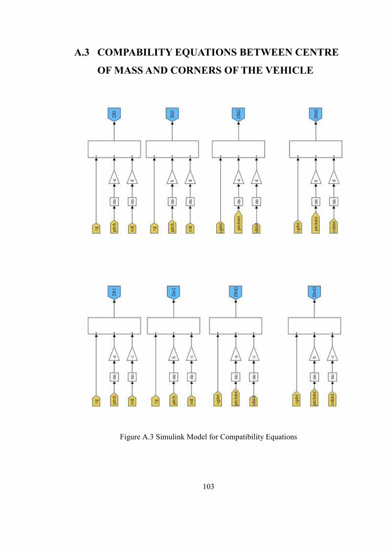
103

A.3 COMPABILITY EQUATIONS BETWEEN CENTRE

OF MASS AND CORNERS OF THE VEHICLE

Figure A.3 Simulink Model for Compatibility Equations

104

A.4 UNSPRUNG MASS MOTION

Figure A.4 Simulink Model of Unsprung Mass Motion

105

A.5 BOUNCE MOTION OF THE VEHICLE

Figure A.5 Simulink Model for Bounce Motion

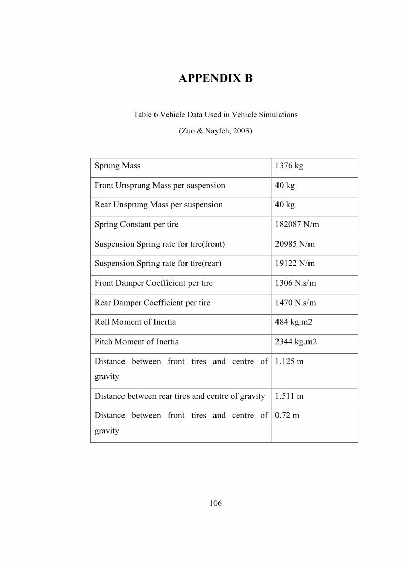
106

B APPENDIX B

Table 6 Vehicle Data Used in Vehicle Simulations

(Zuo & Nayfeh, 2003)

Sprung Mass 1376 kg

Front Unsprung Mass per suspension 40 kg

Rear Unsprung Mass per suspension 40 kg

Spring Constant per tire 182087 N/m

Suspension Spring rate for tire(front) 20985 N/m

Suspension Spring rate for tire(rear) 19122 N/m

Front Damper Coefficient per tire 1306 N.s/m

Rear Damper Coefficient per tire 1470 N.s/m

Roll Moment of Inertia 484 kg.m2

Pitch Moment of Inertia 2344 kg.m2

Distance between front tires and centre of

gravity

1.125 m

Distance between rear tires and centre of gravity 1.511 m

Distance between front tires and centre of

gravity

0.72 m

107

C APPENDIX C

The m-file code used in embedded Matlab/Simulink block to find necessary input

currents for requested damping forces is given here. The logic of this code is briefly:

1-The lookup tables are separately prepared for each current.

2-At a given relative velocity, the damping forces that can be generated at each

current is fed to the embedded function block.

3-By the function of “min”, the two current values which give closest forces to

desired force is found.

4-Linear interpolation is carried between the two currents to find the necessary

currents.

5-As will be discussed if the current is not feasible, the current will be modified.

The code:

function [optcurrent,index,index2,opteski] = fcn(wanted,relvel,f1,f2,f3,f4,f5,f6,f7,f8,f9,current1,current2,current3,current4,current5,current6,current7,current8,current9,count,minlimited,maxlimited,forceminlimit) % This block supports an embeddable subset of the MATLAB language. % See the help menu for details. %the array of forces that can be generated at different current levels at a specific relative velocity: f=[f1 f2 f3 f4 f5 f6 f7 f8 f9]; %the array of available current levels: current=[current1 current2 current3 current4 current5 current6 current7 current8 current9]; delta=[0 0 0 0 0 0 0 0 0]; %each delta represents the difference between demanded force and available force %at a specific current level at a specific relative velocity delta(1)=wanted-f1; delta(2)=wanted-f2; delta(3)=wanted-f3; delta(4)=wanted-f4; delta(5)=wanted-f5; delta(6)=wanted-f6;

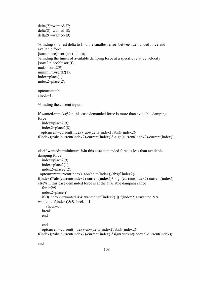
108

delta(7)=wanted-f7; delta(8)=wanted-f8; delta(9)=wanted-f9; %finding smallest delta to find the smallest error between demanded force and available force [sortt,place]=sort(abs(delta)); %finding the limits of available damping force at a specific relative velocity [sortt2,place2]=sort(f); maks=sortt2(9); minimum=sortt2(1); index=place(1); index2=place(2); optcurrent=0; check=1; %finding the current input: if wanted>=maks;%in this case demanded force is more than available damping force index=place2(9); index2=place2(8); optcurrent=current(index)+abs(delta(index))/abs(f(index2)-f(index))*abs(current(index2)-current(index))*-sign(current(index2)-current(index)); elseif wanted<=minimum;%in this case demanded force is less than available damping force index=place2(9); index=place2(1); index2=place2(2); optcurrent=current(index)+abs(delta(index))/abs(f(index2)-f(index))*abs(current(index2)-current(index))*-sign(current(index2)-current(index)); else%in this case demanded force is at the available damping range for i=2:9 index2=place(i); if (f(index)<=wanted && wanted<=f(index2))||( f(index2)<=wanted && wanted<=f(index))&&check==1 check=0; break end end optcurrent=current(index)+abs(delta(index))/abs(f(index2)-f(index))*abs(current(index2)-current(index))*sign(current(index2)-current(index)); end

109

opteski=optcurrent; %Clipping the input current levels: if optcurrent>maxlimited optcurrent=maxlimited; elseif optcurrent<minlimited optcurrent=minlimited; end y = optcurrent;

110

D APPENDIX D

The mass matrix is given as:

fl

bl

fr

fl

xx

yy

m 0 0 0 0 0 0

0 m 0 0 0 0 0

0 0 m 0 0 0 0

0 0 0 m 0 0 0M

0 0 0 0 M 0 0

0 0 0 0 0 I 0

0 0 0 0 0 0 I

=

(D.1)

The stiffness matrix K is written as:

[ ]1 2 3K K K K=

(D.2)

fl1 fl2

bl1 bl2

fr1 fr2

br1 br2

fl2 bl2 fr2 br2

fl2 bl2 fr2 br2

fl2 bl2 fr2 br2

(k k ) 0 0 0

0 (k k ) 0 0

0 0 (k k ) 0

K 0 0 0 (k k )1

k k k k

k a k b k a k b

k d k d k c k c

+ + +

= + − − − −

− − − −

(D.3)

111

fl2 fl2

bl2 bl2

fr 2 fr2

br 2 br2

fl2 bl2 fr 2 br 2 fl2 bl2 fr2 br 2

fl2 bl2 fr 2 br2 fl2 bl2 fr2 br 2

2 2 2 2fl2 bl2 fr 2 br2 fl2 bl2 fr 2 br 2

k k d

k k d

k k c

K k k c2

k k k k k d k d k c k c

k a k b k a k b k ad k bd k ac k bc

k d k d k c k c k d k d k c k c

− −

− − − +

= − + + + + + + − −

− + − + − + + −

+ − − + + +

(D.4)

fl2

bl2

fr 2

br 2

fl2 bl2 fr 2 br 2

fl2 bl2 fr 2 br 2

fl2 bl2 fr 2 br 2

k a

k b

k a

K k b3

k a k b k a k b

2 2 2 2k a k b k a k b

k da k db k ca k cb

− = − − + − + + + + + − + + −

(D.5)

112

E APPENDIX E

Figure E.1 MR Data used in Simulations

DEVELOPMENT OF A CONTROL STRATEGY FOR ROAD …etd.lib.metu.edu.tr/upload/12610392/index.pdf ·...

Documents

Transcript of DEVELOPMENT OF A CONTROL STRATEGY FOR ROAD …etd.lib.metu.edu.tr/upload/12610392/index.pdf ·...