COMPUTATIONAL ANALYSIS OF A MULTISTAGE AXIAL COMPRESSOR

by

CHAITHANYA MAMIDOJU

Presented to the Faculty of the Graduate School of

The University of Texas at Arlington in Partial Fulfillment

of the Requirements

for the Degree of

MASTER OF SCIENCE IN AEROSPACE ENGINEERING

THE UNIVERSITY OF TEXAS AT ARLINGTON

May 2014

Copyright c© by CHAITHANYA MAMIDOJU 2014

All Rights Reserved

To my parents Vanisri and Srinivas Mamidoju

and my brother Kranthi Kumar.

ACKNOWLEDGEMENTS

I express my deep gratitude to my thesis supervisor and mentor Dr. Brian H

Dennis for putting a lot of faith in me and making me feel that I always belonged here.

If only I could achieve half the amount of work he does in a day I would be happy.

Doing research and coursework with him has taught me a lot, especially approaching

a problem and coming up with new ideas.

I am deeply honored and previleged to have two stalwarts of the Mechanical and

Aerospace Department, Dr. Zhen Xue Han and Dr. Bo P Wang in my committee.

I would like to thank my love Yashwanth M Swamy for continuous support and

encouragement throughout my Masters study. I am also grateful to my friends Shilpa

Andam, Mahesan Revathi Sanjay, Ravi Kiran Paturi for for sticking with me through

thick and thin. I would also like to thank all my close friends at UTA for taking the

responsibility of being my local guardians.

Finally, I am thankful to my CFD lab colleagues for being with me and for

their valuable inputs. I would also like to thank my well-wishers for their love and

support. I am also grateful to all my past and present teachers who have a played a

stellar role in shaping up my career.

Above all, I would like to express my deepest gratitude to my parents Srinivas

Mamidoju and Vani Sri Mamidoju, to whom I owe my existence and to my brother

Kranthi Kumar Mamidoju for moral support. They cherished my highs, pulled me

out of the lows, but most importantly, they made me a good human being.

April 21, 2014

iv

ABSTRACT

COMPUTATIONAL ANALYSIS OF A MULTISTAGE AXIAL COMPRESSOR

CHAITHANYA MAMIDOJU, M.S.

The University of Texas at Arlington, 2014

Supervising Professor: Brian H Dennis

Turbomachines are used extensively in Aerospace, Power Generation, and Oil

& Gas Industries. Efficiency of these machines is often an important factor and has

led to the continuous effort to improve the design to achieve better efficiency. The

axial flow compressor is a major component in a gas turbine with the turbine’s overall

performance depending strongly on compressor performance. Traditional analysis of

axial compressors involves throughflow calculations, isolated blade passage analysis,

Quasi-3D blade-to-blade analysis, single-stage (rotor-stator) analysis, and multi-stage

analysis involving larger design cycles.

In the current study, the detailed flow through a 15 stage axial compressor is

analyzed using a 3-D Navier Stokes CFD solver in a parallel computing environment.

Methodology is described for steady state (frozen rotor stator) analysis of one blade

passage per component. Various effects such as mesh type and density, boundary con-

ditions, tip clearance and numerical issues such as turbulence model choice, advection

model choice, and parallel processing performance are analyzed. A high sensitivity

of the predictions to the above was found. Physical explanation to the flow features

v

observed in the computational study are given. The total pressure rise verses mass

flow rate was computed.

vi

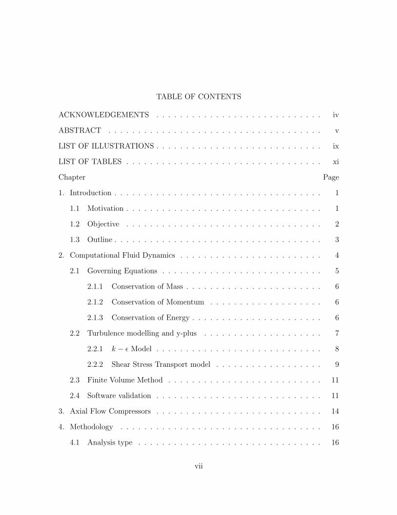
TABLE OF CONTENTS

ACKNOWLEDGEMENTS . . . . . . . . . . . . . . . . . . . . . . . . . . . . iv

ABSTRACT . . . . . . . . . . . . . . . . . . . . . . . . . . . . . . . . . . . . v

LIST OF ILLUSTRATIONS . . . . . . . . . . . . . . . . . . . . . . . . . . . . ix

LIST OF TABLES . . . . . . . . . . . . . . . . . . . . . . . . . . . . . . . . . xi

Chapter Page

1. Introduction . . . . . . . . . . . . . . . . . . . . . . . . . . . . . . . . . . . 1

1.1 Motivation . . . . . . . . . . . . . . . . . . . . . . . . . . . . . . . . . 1

1.2 Objective . . . . . . . . . . . . . . . . . . . . . . . . . . . . . . . . . 2

1.3 Outline . . . . . . . . . . . . . . . . . . . . . . . . . . . . . . . . . . . 3

2. Computational Fluid Dynamics . . . . . . . . . . . . . . . . . . . . . . . . 4

2.1 Governing Equations . . . . . . . . . . . . . . . . . . . . . . . . . . . 5

2.1.1 Conservation of Mass . . . . . . . . . . . . . . . . . . . . . . . 6

2.1.2 Conservation of Momentum . . . . . . . . . . . . . . . . . . . 6

2.1.3 Conservation of Energy . . . . . . . . . . . . . . . . . . . . . . 6

2.2 Turbulence modelling and y-plus . . . . . . . . . . . . . . . . . . . . 7

2.2.1 k − ε Model . . . . . . . . . . . . . . . . . . . . . . . . . . . . 8

2.2.2 Shear Stress Transport model . . . . . . . . . . . . . . . . . . 9

2.3 Finite Volume Method . . . . . . . . . . . . . . . . . . . . . . . . . . 11

2.4 Software validation . . . . . . . . . . . . . . . . . . . . . . . . . . . . 11

3. Axial Flow Compressors . . . . . . . . . . . . . . . . . . . . . . . . . . . . 14

4. Methodology . . . . . . . . . . . . . . . . . . . . . . . . . . . . . . . . . . 16

4.1 Analysis type . . . . . . . . . . . . . . . . . . . . . . . . . . . . . . . 16

vii

4.2 Parallel Processing . . . . . . . . . . . . . . . . . . . . . . . . . . . . 19

4.2.1 Partitioning step . . . . . . . . . . . . . . . . . . . . . . . . . 19

4.2.2 Running step . . . . . . . . . . . . . . . . . . . . . . . . . . . 20

4.3 Preliminary studies . . . . . . . . . . . . . . . . . . . . . . . . . . . . 21

4.3.1 Turbulence Modelling . . . . . . . . . . . . . . . . . . . . . . . 21

4.3.2 Meshing . . . . . . . . . . . . . . . . . . . . . . . . . . . . . . 23

4.4 Computational study using three climatic conditions . . . . . . . . . 24

5. Results and Discussions . . . . . . . . . . . . . . . . . . . . . . . . . . . . 26

5.1 Outlet Static Pressure of 180 kPa for three climatic conditions . . . . 26

5.2 Outlet Static Pressure of 180 kPa, 270 kPa and 300 kPa for winter

condition . . . . . . . . . . . . . . . . . . . . . . . . . . . . . . . . . . 28

6. Concluding Remarks . . . . . . . . . . . . . . . . . . . . . . . . . . . . . . 35

6.1 Future work . . . . . . . . . . . . . . . . . . . . . . . . . . . . . . . . 36

Appendix

A. INPUT CODE FOR PARALLEL PROCESSING . . . . . . . . . . . . . . 37

REFERENCES . . . . . . . . . . . . . . . . . . . . . . . . . . . . . . . . . . . 39

BIOGRAPHICAL STATEMENT . . . . . . . . . . . . . . . . . . . . . . . . . 41

viii

LIST OF ILLUSTRATIONS

Figure Page

1.1 Aeolipile developed by Hero of Alexandria 120 BC . . . . . . . . . . . 1

1.2 48-Stage Axial Flow Compressor made by Parsons in 1904 . . . . . . 2

1.3 Westinghouse J-30 ’yankee’ 10-stage Axial Flow Compressor [1] . . . . 3

2.1 Hub-to-tip and blade-to-blade stream surfaces . . . . . . . . . . . . . 4

2.2 Subdivisions of the near-wall region [6] . . . . . . . . . . . . . . . . . 10

2.3 Plot of Total Pressure ratio and Normalized mass flow of Experimental

Analysis [7] . . . . . . . . . . . . . . . . . . . . . . . . . . . . . . . . . 12

2.4 Plot of Total Pressure ratio and Normalized mass flow of Computational

Analysis . . . . . . . . . . . . . . . . . . . . . . . . . . . . . . . . . . . 13

3.1 A typical multistage axial flow compressor (Rolls-Royce, 1992) [8] . . 14

3.2 Pressure and velocity profiles (Rolls-Royce, 1992) [8] . . . . . . . . . . 15

4.1 Meridonial view of 15 stage compressor . . . . . . . . . . . . . . . . . 17

4.2 Flynn’s Taxonomy [10] . . . . . . . . . . . . . . . . . . . . . . . . . . 18

4.3 Bisection type mesh partitioning [?] . . . . . . . . . . . . . . . . . . . 20

4.4 Parallel computers in CFD lab at UTA . . . . . . . . . . . . . . . . . 21

4.5 Eddy Viscosity of the compressor using κ - ε turbulence model . . . . 22

4.6 Eddy Viscosity of the compressor using SST turbulence model . . . . 22

4.7 Plot of Total Pressure Ratio to Mass Flow Rate . . . . . . . . . . . . 23

4.8 Topology at Mid-span of a Rotor . . . . . . . . . . . . . . . . . . . . . 24

5.1 360 degree view of the compressor . . . . . . . . . . . . . . . . . . . . 26

5.2 Graph of Total Pressure Ratio versus Stage Number . . . . . . . . . . 27

ix

5.3 Pressure contour at 50 percent mid span for Exit Static Pressure = 180

kPa in winter . . . . . . . . . . . . . . . . . . . . . . . . . . . . . . . . 28

5.4 Pressure contour at 50 percent mid span for Exit Static Pressure = 180

kPa in average climate . . . . . . . . . . . . . . . . . . . . . . . . . . . 29

5.5 Pressure contour at 50 percent mid span for Exit Static Pressure = 180

kPa in summer . . . . . . . . . . . . . . . . . . . . . . . . . . . . . . . 29

5.6 Velocity Vector plot at 50 percent mid span for Exit Static Pressure =

180 kPa in winter . . . . . . . . . . . . . . . . . . . . . . . . . . . . . 30

5.7 Velocity vector plot at 50 percent mid span for Exit Static Pressure =

180 kPa in average climate . . . . . . . . . . . . . . . . . . . . . . . . 30

5.8 Velocity vector plot at 50 percent mid span for Exit Static Pressure =

180 kPa in summer . . . . . . . . . . . . . . . . . . . . . . . . . . . . . 31

5.9 Graph of Total Pressure Ratio versus Stage Number for winter condition 32

5.10 Graph of Total Pressure Ratio versus mass flow rate for winter condition 33

5.11 Pressure contour at 50 percent mid span for Exit Static Pressure = 270

kPa in winter . . . . . . . . . . . . . . . . . . . . . . . . . . . . . . . . 33

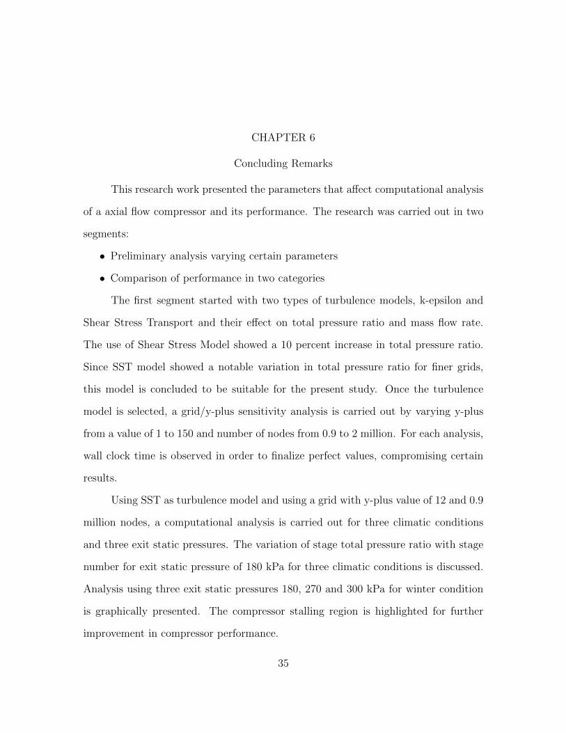
5.12 Velocity vector plot at 50 percent mid span for Exit Static Pressure =

270 kPa in winter . . . . . . . . . . . . . . . . . . . . . . . . . . . . . 34

x

LIST OF TABLES

Table Page

4.1 Number of Blades of Rotor and Stator . . . . . . . . . . . . . . . . . 17

4.2 Total Pressure ratio and computational time for y-plus values and num-

ber of nodes . . . . . . . . . . . . . . . . . . . . . . . . . . . . . . . . . 25

4.3 Boundary conditions of 3 climatic conditions . . . . . . . . . . . . . . 25

5.1 Overall Total Pressure ratio and Inlet mass flow rate for three climatic

conditions . . . . . . . . . . . . . . . . . . . . . . . . . . . . . . . . . . 27

xi

CHAPTER 1

Introduction

1.1 Motivation

Turbomachines are used extensively in Aerospace, Power Generation, and Oil

and Gas Industries. Efficiency of these machines is often an important factor and has

led to the continuous effort to improve the design to achieve better efficiency. From the

man’s beginning to 1700 AD, all the motive power was provided by men or animals.

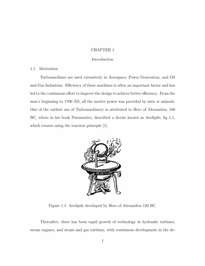
One of the earliest use of Turbomachinery is attributed to Hero of Alexandria, 100

BC, where in his book Pneumatics, described a devise known as Aeolipile, fig 1.1,

which rotates using the reaction principle [1].

Figure 1.1. Aeolipile developed by Hero of Alexandria 120 BC.

Thereafter, there has been rapid growth of technology in hydraulic turbines,

steam engines, and steam and gas turbines, with continuous development in the de-

1

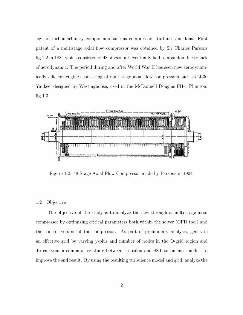
sign of turbomachinery components such as compressors, turbines and fans. First

patent of a multistage axial flow compressor was obtained by Sir Charles Parsons

fig 1.2 in 1884 which consisted of 48 stages but eventually had to abandon due to lack

of aerodynamic. The period during and after World War II has seen new aerodynam-

ically efficient engines consisting of multistage axial flow compressors such as ’J-30

Yankee’ designed by Westinghouse, used in the McDonnell Douglas FH-1 Phantom

fig 1.3.

Figure 1.2. 48-Stage Axial Flow Compressor made by Parsons in 1904.

1.2 Objective

The objective of the study is to analyze the flow through a multi-stage axial

compressor by optimizing critical parameters both within the solver (CFD tool) and

the control volume of the compressor. As part of preliminary analysis, generate

an effective grid by varying y-plus and number of nodes in the O-grid region and

To carryout a comparative study between k-epsilon and SST turbulence models to

improve the end result. By using the resulting turbulence model and grid, analyze the

2

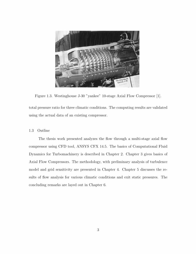
Figure 1.3. Westinghouse J-30 ”yankee” 10-stage Axial Flow Compressor [1].

total pressure ratio for three climatic conditions. The computing results are validated

using the actual data of an existing compressor.

1.3 Outline

The thesis work presented analyzes the flow through a multi-stage axial flow

compressor using CFD tool, ANSYS CFX 14.5. The basics of Computational Fluid

Dynamics for Turbomachinery is described in Chapter 2. Chapter 3 gives basics of

Axial Flow Compressors. The methodology, with preliminary analysis of turbulence

model and grid sensitivity are presented in Chapter 4. Chapter 5 discusses the re-

sults of flow analysis for various climatic conditions and exit static pressures. The

concluding remarks are layed out in Chapter 6.

3

CHAPTER 2

Computational Fluid Dynamics

Computational Fluid Dynamics, commonly known as CFD, is a method of solv-

ing the governing equations of a fluid flow using numerical techniques and computing

power. When compared to traditional methods, such as wind tunnel tests that involve

destructive testing, numerical analysis is much faster, cost effective and feasible. The

usage of these numerical techniques is comparatively higher in the design of Turbo-

machinery than in any other field. The application of the same, dates back to 1940s

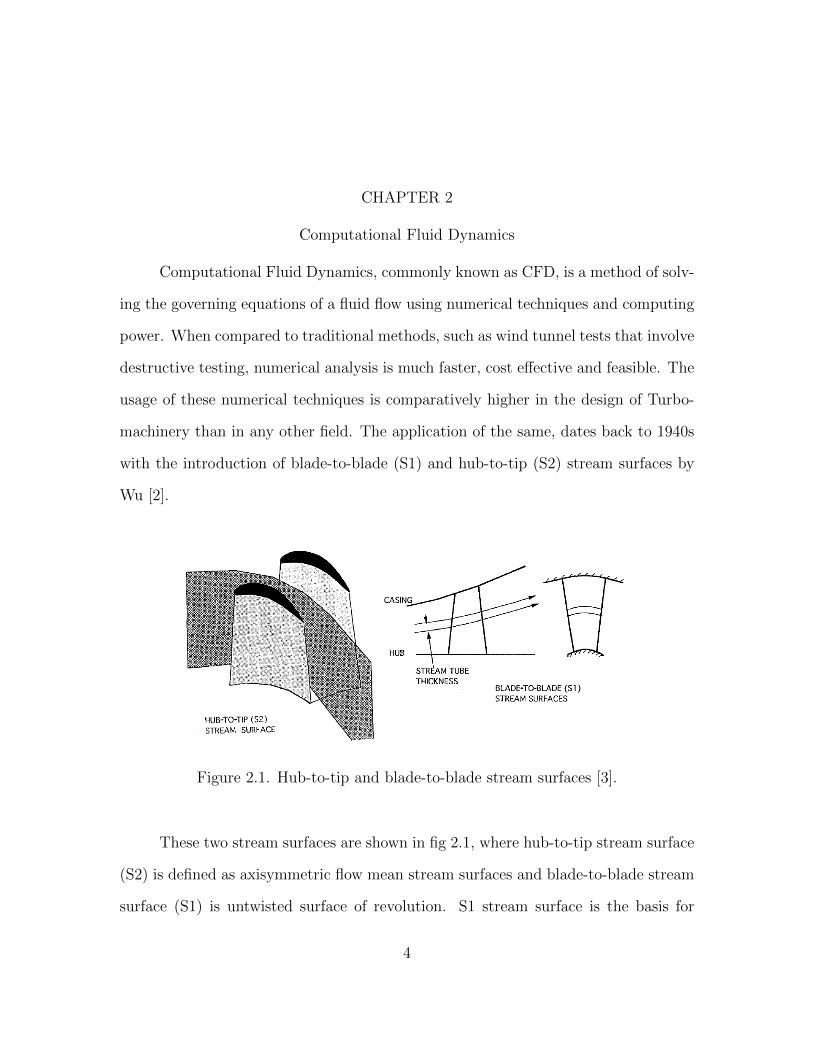
with the introduction of blade-to-blade (S1) and hub-to-tip (S2) stream surfaces by

Wu [2].

Figure 2.1. Hub-to-tip and blade-to-blade stream surfaces [3].

These two stream surfaces are shown in fig 2.1, where hub-to-tip stream surface

(S2) is defined as axisymmetric flow mean stream surfaces and blade-to-blade stream

surface (S1) is untwisted surface of revolution. S1 stream surface is the basis for

4

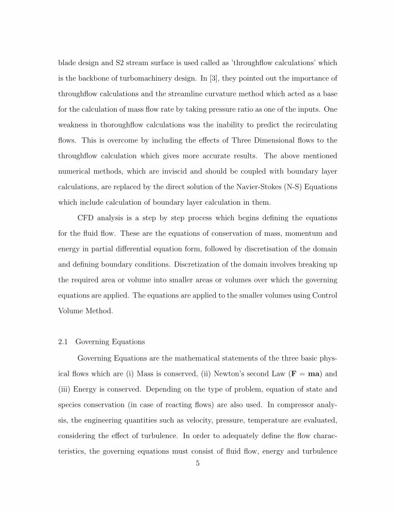
blade design and S2 stream surface is used called as ’throughflow calculations’ which

is the backbone of turbomachinery design. In [3], they pointed out the importance of

throughflow calculations and the streamline curvature method which acted as a base

for the calculation of mass flow rate by taking pressure ratio as one of the inputs. One

weakness in thoroughflow calculations was the inability to predict the recirculating

flows. This is overcome by including the effects of Three Dimensional flows to the

throughflow calculation which gives more accurate results. The above mentioned

numerical methods, which are inviscid and should be coupled with boundary layer

calculations, are replaced by the direct solution of the Navier-Stokes (N-S) Equations

which include calculation of boundary layer calculation in them.

CFD analysis is a step by step process which begins defining the equations

for the fluid flow. These are the equations of conservation of mass, momentum and

energy in partial differential equation form, followed by discretisation of the domain

and defining boundary conditions. Discretization of the domain involves breaking up

the required area or volume into smaller areas or volumes over which the governing

equations are applied. The equations are applied to the smaller volumes using Control

Volume Method.

2.1 Governing Equations

Governing Equations are the mathematical statements of the three basic phys-

ical flows which are (i) Mass is conserved, (ii) Newton’s second Law (F = ma) and

(iii) Energy is conserved. Depending on the type of problem, equation of state and

species conservation (in case of reacting flows) are also used. In compressor analy-

sis, the engineering quantities such as velocity, pressure, temperature are evaluated,

considering the effect of turbulence. In order to adequately define the flow charac-

teristics, the governing equations must consist of fluid flow, energy and turbulence

5

models. Descriptions of the equations used and an explanation of how these are

applied is explained below. For the derivations of each equation, refer to [4]

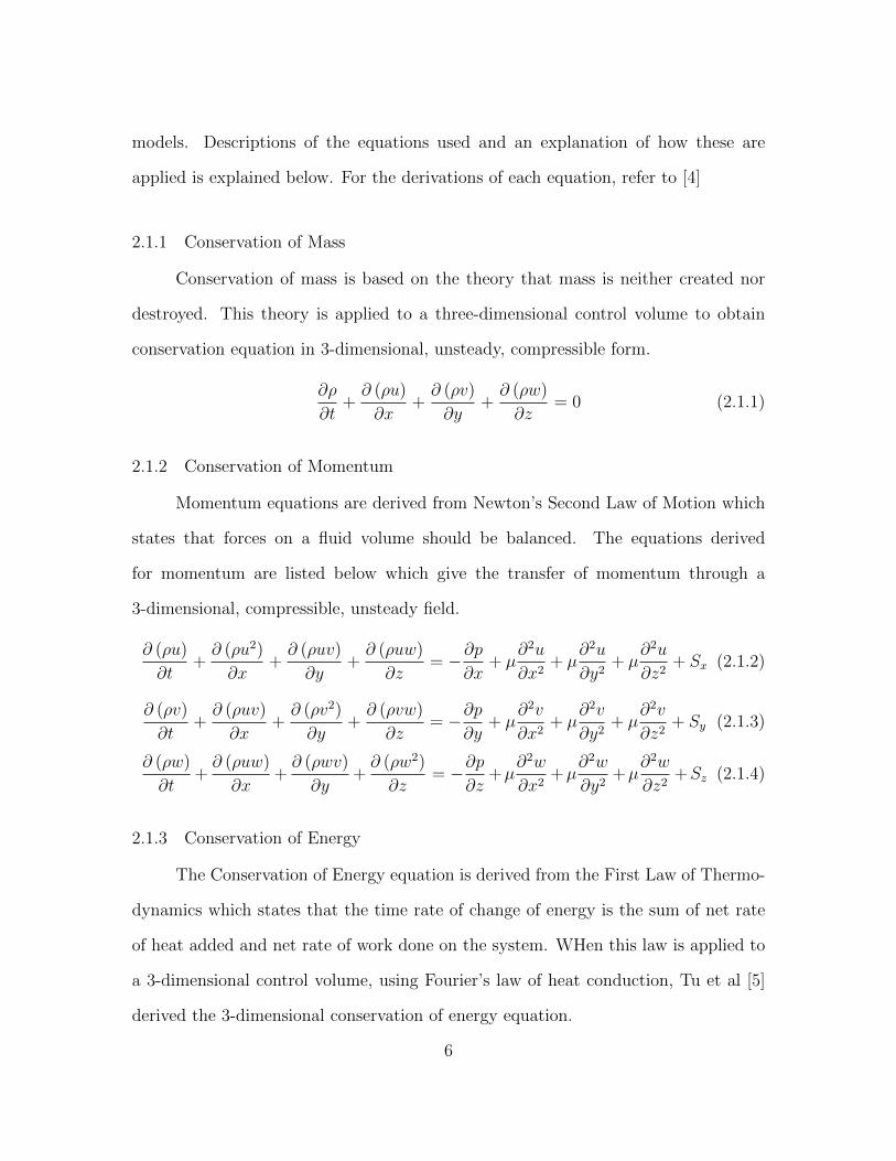
2.1.1 Conservation of Mass

Conservation of mass is based on the theory that mass is neither created nor

destroyed. This theory is applied to a three-dimensional control volume to obtain

conservation equation in 3-dimensional, unsteady, compressible form.

∂ρ

∂t+∂ (ρu)

∂x+∂ (ρv)

∂y+∂ (ρw)

∂z= 0 (2.1.1)

2.1.2 Conservation of Momentum

Momentum equations are derived from Newton’s Second Law of Motion which

states that forces on a fluid volume should be balanced. The equations derived

for momentum are listed below which give the transfer of momentum through a

3-dimensional, compressible, unsteady field.

∂ (ρu)

∂t+∂ (ρu2)

∂x+∂ (ρuv)

∂y+∂ (ρuw)

∂z= −∂p

∂x+ µ

∂2u

∂x2+ µ

∂2u

∂y2+ µ

∂2u

∂z2+ Sx (2.1.2)

∂ (ρv)

∂t+∂ (ρuv)

∂x+∂ (ρv2)

∂y+∂ (ρvw)

∂z= −∂p

∂y+ µ

∂2v

∂x2+ µ

∂2v

∂y2+ µ

∂2v

∂z2+ Sy (2.1.3)

∂ (ρw)

∂t+∂ (ρuw)

∂x+∂ (ρwv)

∂y+∂ (ρw2)

∂z= −∂p

∂z+µ

∂2w

∂x2+µ

∂2w

∂y2+µ

∂2w

∂z2+Sz (2.1.4)

2.1.3 Conservation of Energy

The Conservation of Energy equation is derived from the First Law of Thermo-

dynamics which states that the time rate of change of energy is the sum of net rate

of heat added and net rate of work done on the system. WHen this law is applied to

a 3-dimensional control volume, using Fourier’s law of heat conduction, Tu et al [5]

derived the 3-dimensional conservation of energy equation.

6

∂T

∂t+∂uT

∂x+∂vT

∂y+∂wT

∂z=

k

ρCp

[∂2T

∂x2+∂2T

∂y2+∂2T

∂z2

]+

1

ρCp

∂p

∂t+

Φ

ρCp(2.1.5)

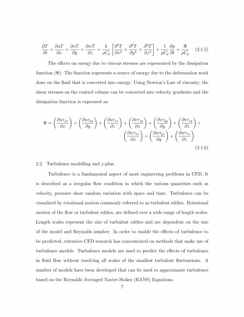
The effects on energy due to viscous stresses are represented by the dissipation

function (Φ). The function represents a source of energy due to the deformation work

done on the fluid that is converted into energy. Using Newton’s Law of viscosity, the

shear stresses on the control volume can be converted into velocity gradients and the

dissipation function is expressed as:

Φ =

(∂uτxx∂x

)+

(∂uτyx∂y

)+

(∂uτzx∂z

)+

(∂vτxy∂x

)+

(∂vτyy∂y

)+

(∂vτzy∂z

)+(

∂wτxz∂x

)+

(∂wτyz∂y

)+

(∂wτzz∂z

)(2.1.6)

2.2 Turbulence modelling and y-plus

Turbulence is a fundamental aspect of most engineering problems in CFD. It

is described as a irregular flow condition in which the various quantities such as

velocity, pressure show random variation with space and time. Turbulence can be

visualized by rotational motion commonly referred to as turbulent eddies. Rotational

motion of the flow or turbulent eddies, are defined over a wide range of length scales.

Length scales represent the size of turbulent eddies and are dependent on the size

of the model and Reynolds number. In order to enable the effects of turbulence to

be predicted, extensive CFD research has concentrated on methods that make use of

turbulence models. Turbulence models are used to predict the effects of turbulence

in fluid flow without resolving all scales of the smallest turbulent fluctuations. A

number of models have been developed that can be used to approximate turbulence

based on the Reynolds Averaged Navier-Stokes (RANS) Equations.

7

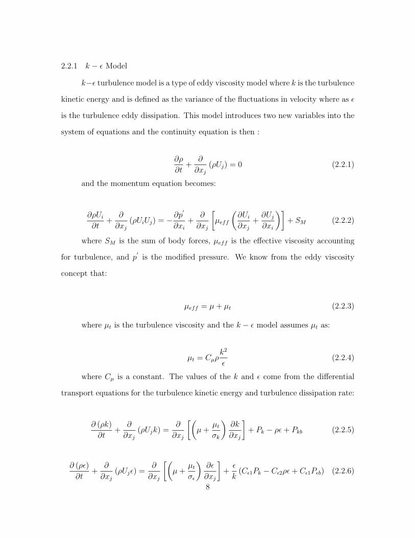
2.2.1 k − ε Model

k−ε turbulence model is a type of eddy viscosity model where k is the turbulence

kinetic energy and is defined as the variance of the fluctuations in velocity where as ε

is the turbulence eddy dissipation. This model introduces two new variables into the

system of equations and the continuity equation is then :

∂ρ

∂t+

∂

∂xj(ρUj) = 0 (2.2.1)

and the momentum equation becomes:

∂ρUi∂t

+∂

∂xj(ρUiUj) = −∂p

′

∂xi+

∂

∂xj

[µeff

(∂Ui∂xj

+∂Uj∂xi

)]+ SM (2.2.2)

where SM is the sum of body forces, µeff is the effective viscosity accounting

for turbulence, and p′

is the modified pressure. We know from the eddy viscosity

concept that:

µeff = µ+ µt (2.2.3)

where µt is the turbulence viscosity and the k − ε model assumes µt as:

µt = Cµρk2

ε(2.2.4)

where Cµ is a constant. The values of the k and ε come from the differential

transport equations for the turbulence kinetic energy and turbulence dissipation rate:

∂ (ρk)

∂t+

∂

∂xj(ρUjk) =

∂

∂xj

[(µ+

µtσk

)∂k

∂xj

]+ Pk − ρε+ Pkb (2.2.5)

∂ (ρε)

∂t+

∂

∂xj(ρUjε) =

∂

∂xj

[(µ+

µtσε

)∂ε

∂xj

]+ε

k(Cε1Pk − Cε2ρε+ Cε1Pεb) (2.2.6)

8

where Cε1, Cε2, σk and σε are constants.

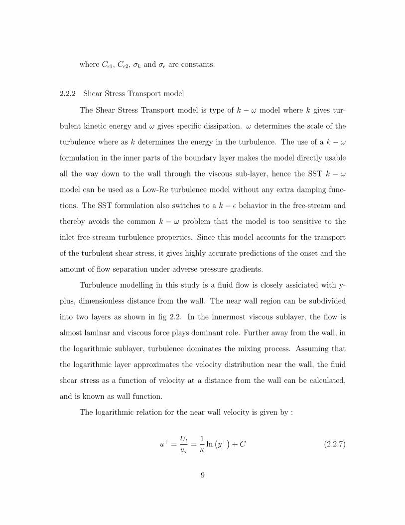
2.2.2 Shear Stress Transport model

The Shear Stress Transport model is type of k − ω model where k gives tur-

bulent kinetic energy and ω gives specific dissipation. ω determines the scale of the

turbulence where as k determines the energy in the turbulence. The use of a k − ω

formulation in the inner parts of the boundary layer makes the model directly usable

all the way down to the wall through the viscous sub-layer, hence the SST k − ω

model can be used as a Low-Re turbulence model without any extra damping func-

tions. The SST formulation also switches to a k − ε behavior in the free-stream and

thereby avoids the common k − ω problem that the model is too sensitive to the

inlet free-stream turbulence properties. Since this model accounts for the transport

of the turbulent shear stress, it gives highly accurate predictions of the onset and the

amount of flow separation under adverse pressure gradients.

Turbulence modelling in this study is a fluid flow is closely assiciated with y-

plus, dimensionless distance from the wall. The near wall region can be subdivided

into two layers as shown in fig 2.2. In the innermost viscous sublayer, the flow is

almost laminar and viscous force plays dominant role. Further away from the wall, in

the logarithmic sublayer, turbulence dominates the mixing process. Assuming that

the logarithmic layer approximates the velocity distribution near the wall, the fluid

shear stress as a function of velocity at a distance from the wall can be calculated,

and is known as wall function.

The logarithmic relation for the near wall velocity is given by :

u+ =Utuτ

=1

κln(y+)

+ C (2.2.7)

9

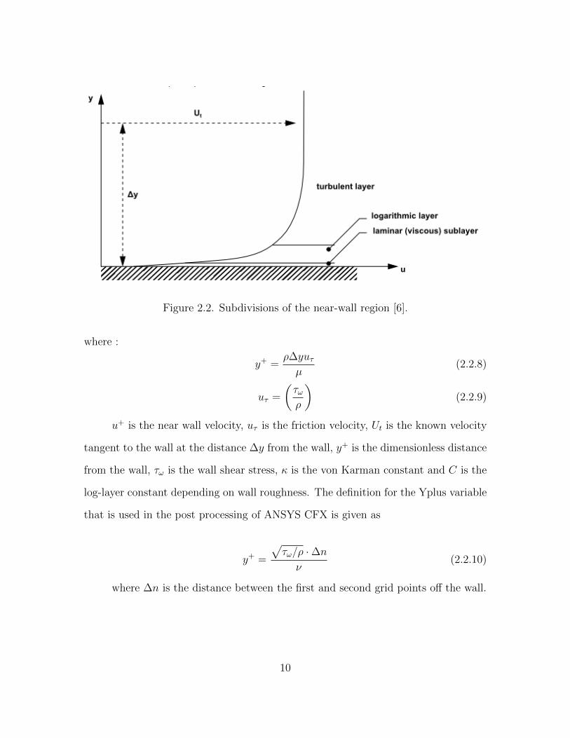
Figure 2.2. Subdivisions of the near-wall region [6].

where :

y+ =ρ∆yuτµ

(2.2.8)

uτ =

(τωρ

)(2.2.9)

u+ is the near wall velocity, uτ is the friction velocity, Ut is the known velocity

tangent to the wall at the distance ∆y from the wall, y+ is the dimensionless distance

from the wall, τω is the wall shear stress, κ is the von Karman constant and C is the

log-layer constant depending on wall roughness. The definition for the Yplus variable

that is used in the post processing of ANSYS CFX is given as

y+ =

√τω/ρ · ∆n

ν(2.2.10)

where ∆n is the distance between the first and second grid points off the wall.

10

2.3 Finite Volume Method

Once the governing equations are defined, the domain is discretized for the

equations to be applied. The Finite Volume Method (FVM) is the most widely ap-

plied method in CFD. The FVM discretizes the governing equations directly in the

physical space. Since this method works with the control volume and not the grid

intersection points, it can accommodate any type of grid, structured or unstructured.

The conservation equations are integrated over each control volume, and Gauss’ Di-

vergence Theorem is applied to evaluate cell centered values from values at the cell

faces. The variable values at the cell faces are averaged values from the adjacent cell

centers (First-Order Upwind) or the adjacent two cells (Second Order Upwind). Since

the discrete equations are more diffuse than the original differential equations, the

First Order Upwinding Method (FOU) introduces some numerical diffusion and even

more where large gradients exist. However, the FOU method converges faster than

SOU methods and can be used with higher Courant Numbers to increase convergence

rates. The FOU scheme is utilized in this analysis since it is a design analysis and

the convergence rate (or time) is a major factor in retrieving a design solution. Refer

to Tu, et al [5] for more information.

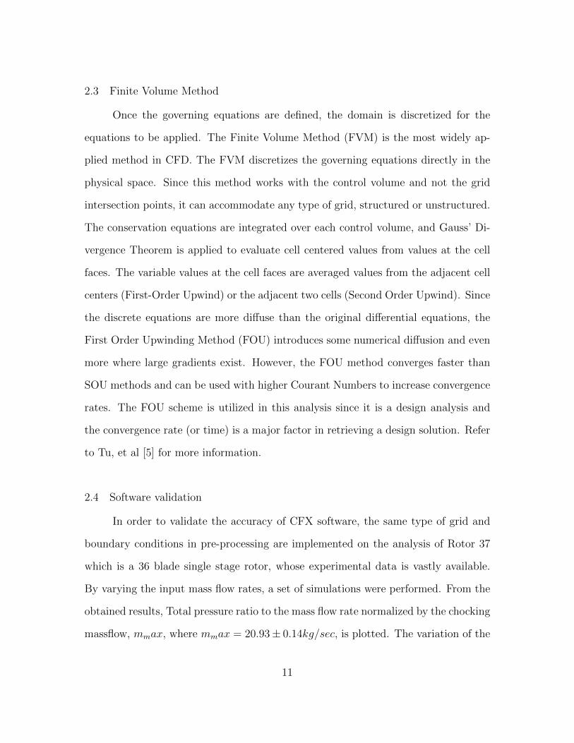
2.4 Software validation

In order to validate the accuracy of CFX software, the same type of grid and

boundary conditions in pre-processing are implemented on the analysis of Rotor 37

which is a 36 blade single stage rotor, whose experimental data is vastly available.

By varying the input mass flow rates, a set of simulations were performed. From the

obtained results, Total pressure ratio to the mass flow rate normalized by the chocking

massflow, mmax, where mmax = 20.93± 0.14kg/sec, is plotted. The variation of the

11

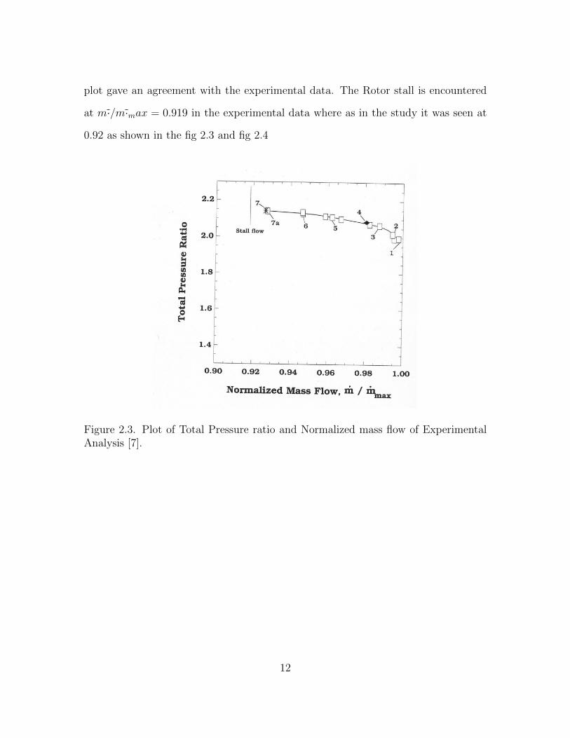
plot gave an agreement with the experimental data. The Rotor stall is encountered

at m·/m·max = 0.919 in the experimental data where as in the study it was seen at

0.92 as shown in the fig 2.3 and fig 2.4

Figure 2.3. Plot of Total Pressure ratio and Normalized mass flow of ExperimentalAnalysis [7].

12

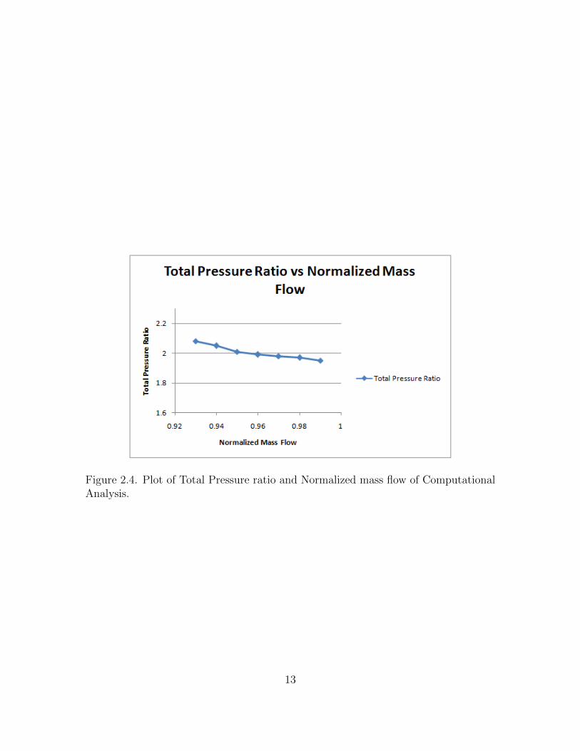
Figure 2.4. Plot of Total Pressure ratio and Normalized mass flow of ComputationalAnalysis.

13

CHAPTER 3

Axial Flow Compressors

An Axial Flow compressors is typically made of alternating rows of rotors (ro-

tating blades) and stators (stationary blades) as shown in fig 3.1. The first stationary

row is called inlet guide vanes or IGV. Each successive rotor-stator pair is called a

compressor stage.

Figure 3.1. A typical multistage axial flow compressor (Rolls-Royce, 1992) [8].

The working of a compressor is based on the energy exchanges. Consider the

Bernoulli Equation, where PT is the stagnation pressure, a measure of the total

energy carried in the flow, p is the static pressure, a measure of the internal energy,

and the velocity terms, a measure of kinetic energy associated with three components

of velocity, u is radial, v is tangential, w is axial.

14

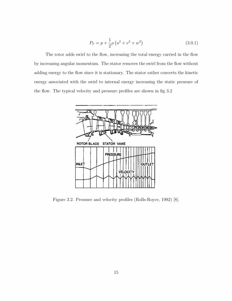
PT = p+1

2ρ(u2 + v2 + w2

)(3.0.1)

The rotor adds swirl to the flow, increasing the total energy carried in the flow

by increasing angular momentum. The stator removes the swirl from the flow without

adding energy to the flow since it is stationary. The stator rather converts the kinetic

energy associated with the swirl to internal energy increasing the static pressure of

the flow. The typical velocity and pressure profiles are shown in fig 3.2

Figure 3.2. Pressure and velocity profiles (Rolls-Royce, 1992) [8].

15

CHAPTER 4

Methodology

Computational Fluid Dynamics has been used to analyze the flow through ro-

tating machines in general and axial compressors particularly. In current study, a

15 stage axial flow compressor is analyzed using commercial CFD package CFX 14.5

which has integrated pre and post processing capabilities. The compressor consists

of 31 blade rows, with an inlet guide vane (IGV) used for blast furnace [9]. The

compressor flow path is that of a constant diameter. The hub-tip radius ratio ranges

from 0.615 at the inlet blade to 0.798 at the outlet blade. The airfoils of all the 31

blade rows belong to NACA 65-series and the rotor blades have constant airfoil shape

from hub to tip. The number of blades in each row of rotor and stator are given in

the Table 4.1. The IGV, first and second stage stator constitutes of twisted blades

while the rest are straight as shown in fig 4.1.

A 3D Navier Stokes solver, Ansys CFX [6] is used to analyse. The flow solver

consists of three stages. The pre-processing where, geometry, mesh, boundary condi-

tions are set. THe defined file is then solved using serial or a parallel solver and once

the solver converges, the results file is then analysed in post- processing segment.

4.1 Analysis type

Steady State analysis where model flows do not change with time is carried out

in this study. Here the steady conditions are assumed to have been reached after

a relatively long interval. Frozen rotor simulations are implemented where rotating

and stationary parts have a fixed relative position. This type of simulation is also

16

Table 4.1. Number of Blades of Rotor and Stator

Rotor Number of Blades Stator Number of Blades0 28

1 27 1 282 27 2 363 33 3 304 31 4 305 31 5 266 37 6 267 37 7 288 37 8 369 37 9 3610 47 10 3611 47 11 3612 47 12 3613 47 13 3614 47 14 3615 47 15 36

Figure 4.1. Meridonial view of 15 stage compressor.

17

called multiple frame of reference approach where a frame transformation is done to

include the rotating effect on the rotating sections. With a frozen-rotor simulation

rotating wakes, secondary flows, leading edge pressure increases etc will always stay

in exactly the same positions which makes the simulation dependent on exactly how

the rotors and the stators are positioned. When compared to mixing plane approach

where a coupling between tangential averages on both sides of the interface between

rotor and stator is done, a frozen rotor approach provides a local coupling imposing

the local flow conditions from one row to the other.

Figure 4.2. Flynn’s Taxonomy [10].

18

4.2 Parallel Processing

Complex flow fields in turbomachine require high performance computer to solve

governing equations to meet memory, cost and time constraints. Parallel computing is

the simultaneous operation of multiple computational tasks on a computer system. It

has been an integral part of computing system from their beginning with the earliest

reference appears to be the description by L. Menabrea of Charles Babbages computer

[11]. For many years the taxonomy of Flynn has been used for the classification of high

performance computers.[12]. This classification is based on the way instruction and

data streams are handled. The classification is shown in fig 4.2.SISD refers to Single

Instruction Single Data Stream, the class of a traditional computer like PC. SIMD is

the Single Instruction Multiple Data Stream type architecture which is implemented

by the solver used in research. This model runs identical versions of the code on

one or more processors. The third type is MISD which is Multiple Instruction Single

Data Stream type, used in Space Shuttle flight control computer. Parallel processing

is explained with respect to CFX solver. The overall parallel run procedure is divided

in two two categories : (1) Partitioning step and (2) Running step.

4.2.1 Partitioning step

Partitioning is the process of dividing the mesh into a number of partitions each

of which may be solved by a separate processor. Several partitioning methods have

been developed, but most are based on recursive bisection and differ only in the bi-

section step. The original mesh is first decomposed into two meshes of approximately

equal size. The decomposition is then repeated recursively until the required number

of partitions is obtained. The fig 4.3 describes the process. MeTiS Partitioning model

based on multilevel k-way algorithm are implemented in current study.

19

Figure 4.3. Bisection type mesh partitioning [6].

4.2.2 Running step

A running step is where the mesh partitions are solved using separate processes

(a master and one or more slave partitions), with each process working on its own par-

tition. Simulation control and user interaction, as well as the input/output phases

of parallel run are performed by master process. This approach guarantees good

parallel performance and scalability of the parallel code. Communication between

processes during parallel run is performed using PVM (Parallel Virtual Machine) or

MPI (Message Passing Interface) libraries. For homogeneous distributed machines

and multi-processor machines, MPI has been shown to give improved parallel effi-

ciency over the PVM libraries. Detailed information can be obtained in any Parallel

Computing texts books.

The parallel computers fig 4.4 available in Computational Fluid Dynamics Lab-

oratory of University of Texas at Arlington are used for the analysis. There are a

total of nine nodes, each consisting of four cores. The Linux operating system is used

20

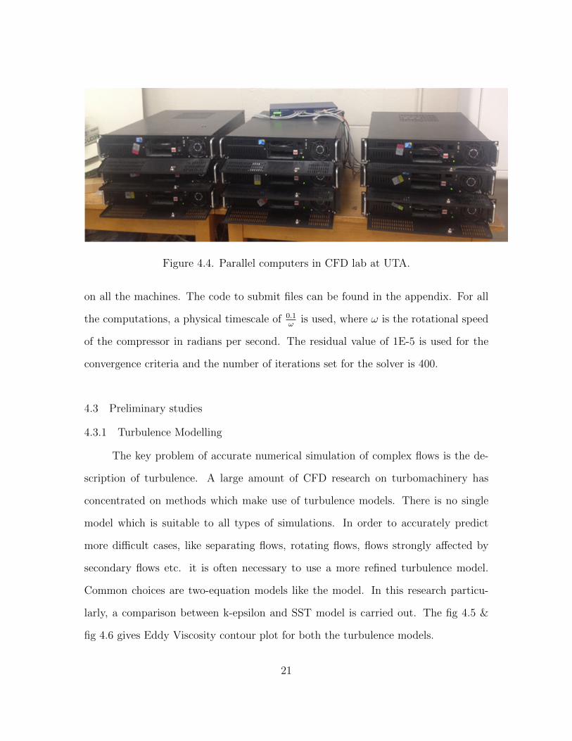
Figure 4.4. Parallel computers in CFD lab at UTA.

on all the machines. The code to submit files can be found in the appendix. For all

the computations, a physical timescale of 0.1ω

is used, where ω is the rotational speed

of the compressor in radians per second. The residual value of 1E-5 is used for the

convergence criteria and the number of iterations set for the solver is 400.

4.3 Preliminary studies

4.3.1 Turbulence Modelling

The key problem of accurate numerical simulation of complex flows is the de-

scription of turbulence. A large amount of CFD research on turbomachinery has

concentrated on methods which make use of turbulence models. There is no single

model which is suitable to all types of simulations. In order to accurately predict

more difficult cases, like separating flows, rotating flows, flows strongly affected by

secondary flows etc. it is often necessary to use a more refined turbulence model.

Common choices are two-equation models like the model. In this research particu-

larly, a comparison between k-epsilon and SST model is carried out. The fig 4.5 &

fig 4.6 gives Eddy Viscosity contour plot for both the turbulence models.

21

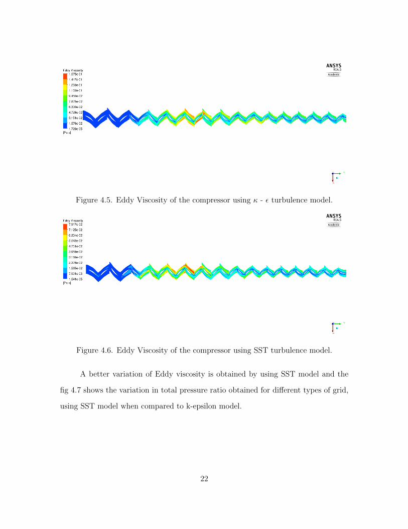
Figure 4.5. Eddy Viscosity of the compressor using κ - ε turbulence model.

Figure 4.6. Eddy Viscosity of the compressor using SST turbulence model.

A better variation of Eddy viscosity is obtained by using SST model and the

fig 4.7 shows the variation in total pressure ratio obtained for different types of grid,

using SST model when compared to k-epsilon model.

22

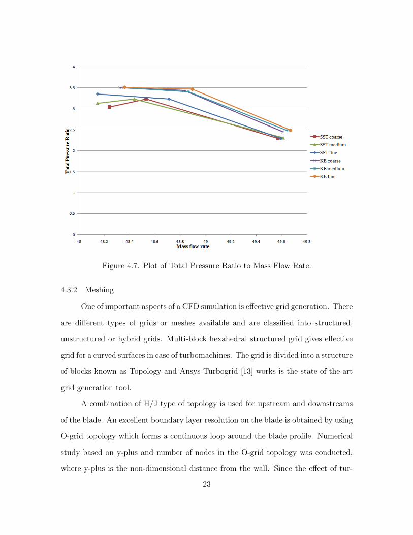
Figure 4.7. Plot of Total Pressure Ratio to Mass Flow Rate.

4.3.2 Meshing

One of important aspects of a CFD simulation is effective grid generation. There

are different types of grids or meshes available and are classified into structured,

unstructured or hybrid grids. Multi-block hexahedral structured grid gives effective

grid for a curved surfaces in case of turbomachines. The grid is divided into a structure

of blocks known as Topology and Ansys Turbogrid [13] works is the state-of-the-art

grid generation tool.

A combination of H/J type of topology is used for upstream and downstreams

of the blade. An excellent boundary layer resolution on the blade is obtained by using

O-grid topology which forms a continuous loop around the blade profile. Numerical

study based on y-plus and number of nodes in the O-grid topology was conducted,

where y-plus is the non-dimensional distance from the wall. Since the effect of tur-

23

Figure 4.8. Topology at Mid-span of a Rotor.

bulence and boundary layer changes are predominant in regions closer to the blade,

the refinement of mesh is carried out in o-grid region. Three nodes are used for each

analysis and total time for the simulation is also given. The analysis is carried out us-

ing SST turbulence model, which assumes linear wall function at lower y-plus values.

The Table 4.2 gives the Total pressure ratio for a set of y-plus values and number of

nodes in O-grid. The lower the y-plus value, more resolution of the viscous sublayer

is obtained. A yplus value of 12 is chosen for further analysis since the desired out-

puts do not much vary from yplus value of 1 and choosing the former, also lowers

computational time and complexity.

4.4 Computational study using three climatic conditions

The Shear Stress Transport as the turbulence model with a y-plus of 12 and

number of o-grid elements of 11 for meshing, are used for the analysis of compressor

24

Table 4.2. Total Pressure ratio and computational time for y-plus values and numberof nodes

No. of O-gridElements (N) No. of nodes Y-plus 1 Y-plus 12 Y-plus 70 Y-plus 150

in million11 0.9 3.2334 3.2312 3.2404 3.2471

3.5 hrs 3.5 hrs 3.5 hrs 3.5 hrs15 1.1 3.2339 3.2317 3.2420 3.2477

3.25 hrs 4 hrs 4 hrs 4.25 hrs20 1.3 3.2347 3.2328 3.2431 3.2482

4.5 hrs 4.5 hrs 5 hrs 5 hrs25 1.6 3.2365 3.2335 3.2440 3.2480

4.5 hrs 5 hrs 5 hrs 5 hrs32 2.0 3.2371 3.2347 3.2401 3.2471

5.5 hrs 5.5 hrs 5.5 hrs 5.5 hrs

for three sets of conditions. The details of the boundary conditions are given in

Table 4.3 and outlet Static pressures of 180, 270, 300, 330, 400, 480 are applied for

each of the climatic conditions to examine the performance.

Table 4.3. Boundary conditions of 3 climatic conditions

Boundary Winter Average Summerconditions

Inlet total pressure 90 89 88(kPa)

Inlet total temperature 257.15 303.45 281.25(K)

Rotation speed 5100 5100 5100rpm

25

CHAPTER 5

Results and Discussions

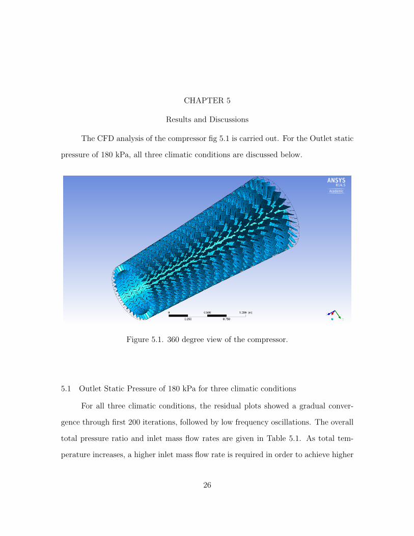
The CFD analysis of the compressor fig 5.1 is carried out. For the Outlet static

pressure of 180 kPa, all three climatic conditions are discussed below.

Figure 5.1. 360 degree view of the compressor.

5.1 Outlet Static Pressure of 180 kPa for three climatic conditions

For all three climatic conditions, the residual plots showed a gradual conver-

gence through first 200 iterations, followed by low frequency oscillations. The overall

total pressure ratio and inlet mass flow rates are given in Table 5.1. As total tem-

perature increases, a higher inlet mass flow rate is required in order to achieve higher

26

performance. One way to increase the mass flow rate is by varying stagger angles of

the stators.

Table 5.1. Overall Total Pressure ratio and Inlet mass flow rate for three climaticconditions

Climatic conditions Total Pressure Ratio Inlet mass flow ratein kg/s

Winter 2.2956 49.5951Average 2.2760 44.7284Summer 2.2722 40.9430

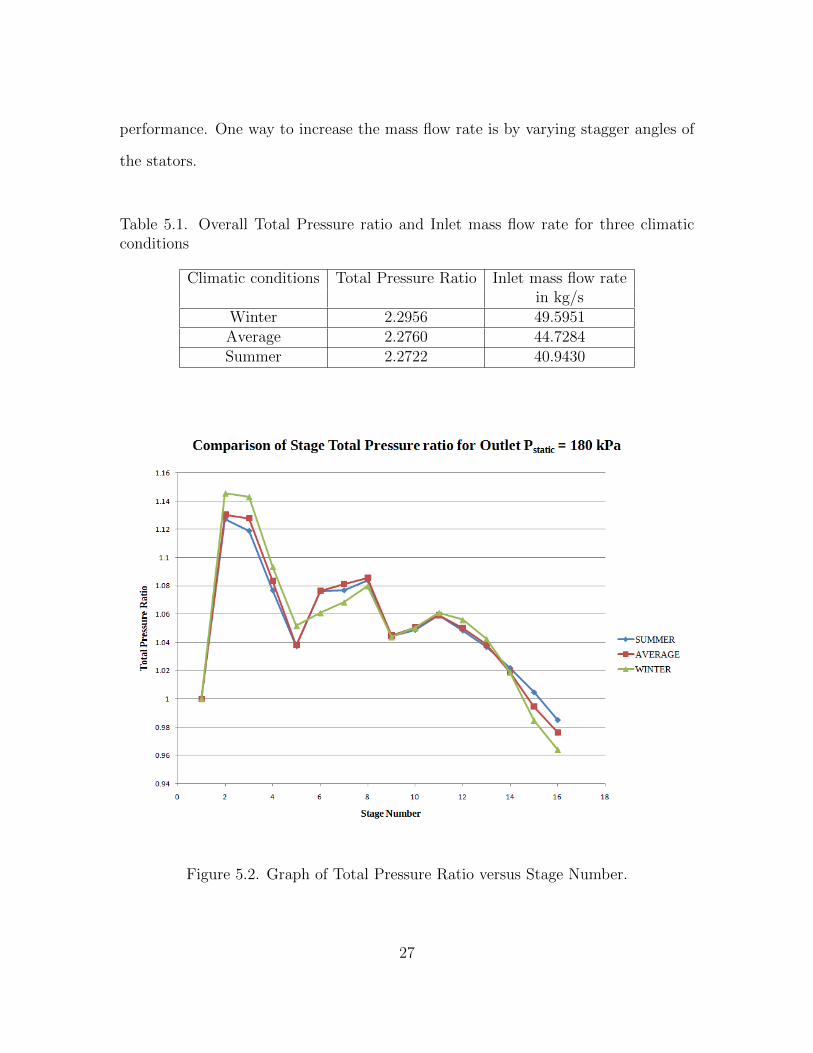
Figure 5.2. Graph of Total Pressure Ratio versus Stage Number.

27

The fig 5.2 shows plot of Total Pressure ratio versus stage number for all three

conditions. For all three conditions, it is seen that variation of total pressure ratio

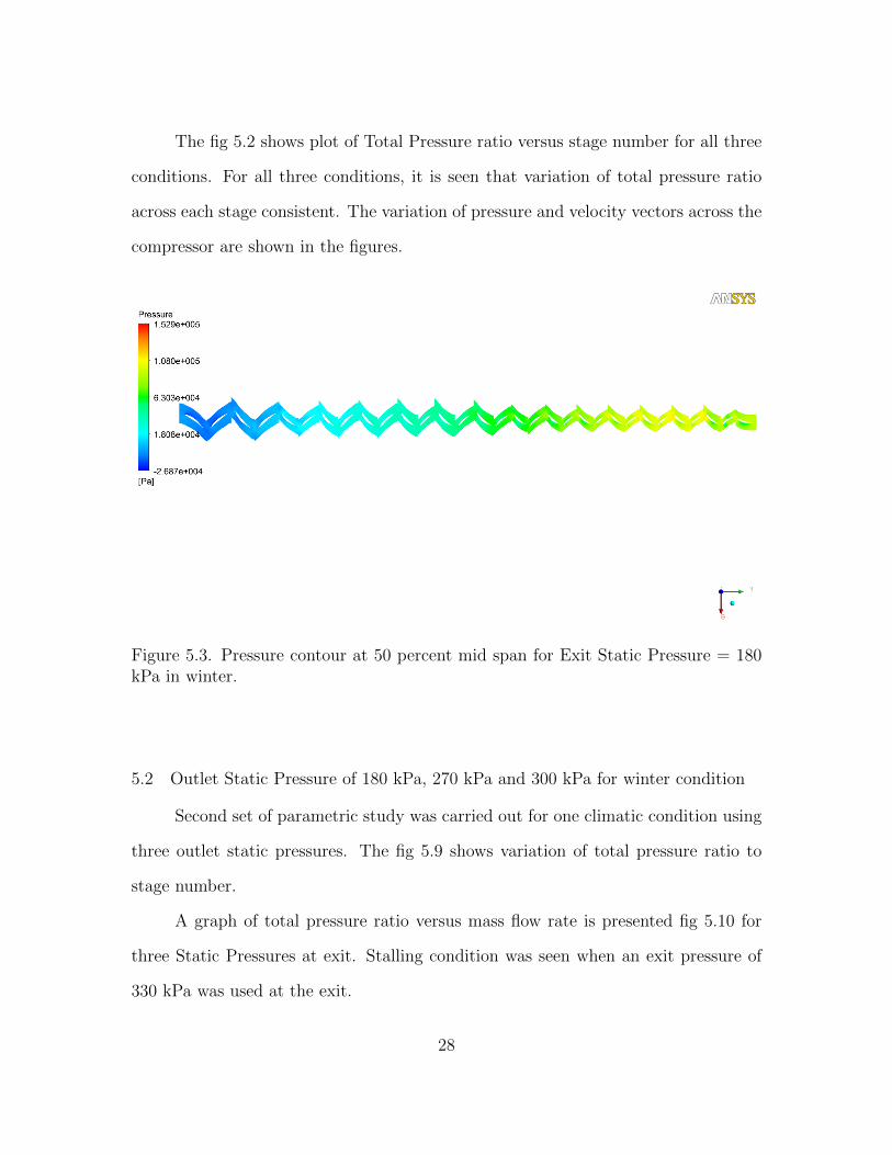
across each stage consistent. The variation of pressure and velocity vectors across the

compressor are shown in the figures.

Figure 5.3. Pressure contour at 50 percent mid span for Exit Static Pressure = 180kPa in winter.

5.2 Outlet Static Pressure of 180 kPa, 270 kPa and 300 kPa for winter condition

Second set of parametric study was carried out for one climatic condition using

three outlet static pressures. The fig 5.9 shows variation of total pressure ratio to

stage number.

A graph of total pressure ratio versus mass flow rate is presented fig 5.10 for

three Static Pressures at exit. Stalling condition was seen when an exit pressure of

330 kPa was used at the exit.

28

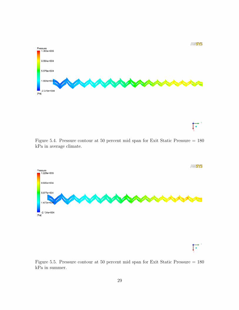
Figure 5.4. Pressure contour at 50 percent mid span for Exit Static Pressure = 180kPa in average climate.

Figure 5.5. Pressure contour at 50 percent mid span for Exit Static Pressure = 180kPa in summer.

29

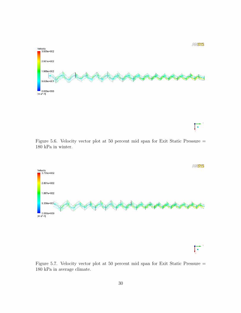
Figure 5.6. Velocity vector plot at 50 percent mid span for Exit Static Pressure =180 kPa in winter.

Figure 5.7. Velocity vector plot at 50 percent mid span for Exit Static Pressure =180 kPa in average climate.

30

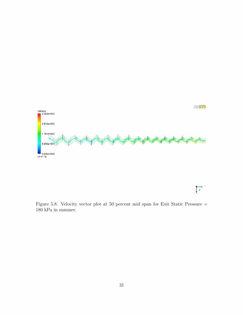
Figure 5.8. Velocity vector plot at 50 percent mid span for Exit Static Pressure =180 kPa in summer.

31

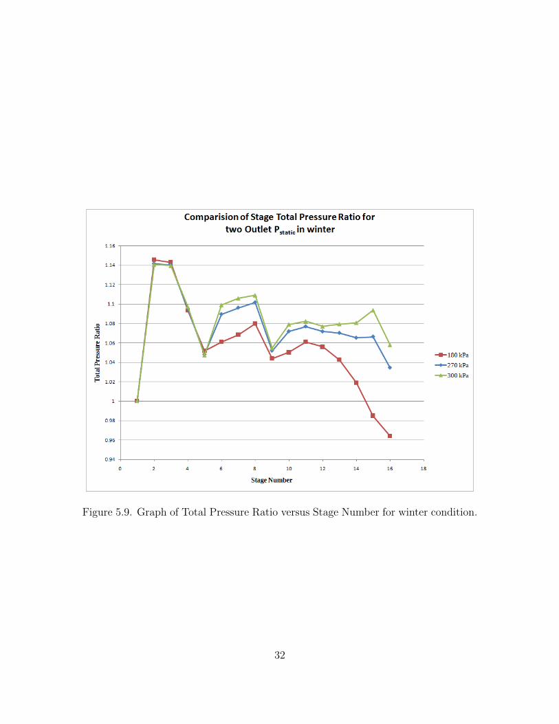
Figure 5.9. Graph of Total Pressure Ratio versus Stage Number for winter condition.

32

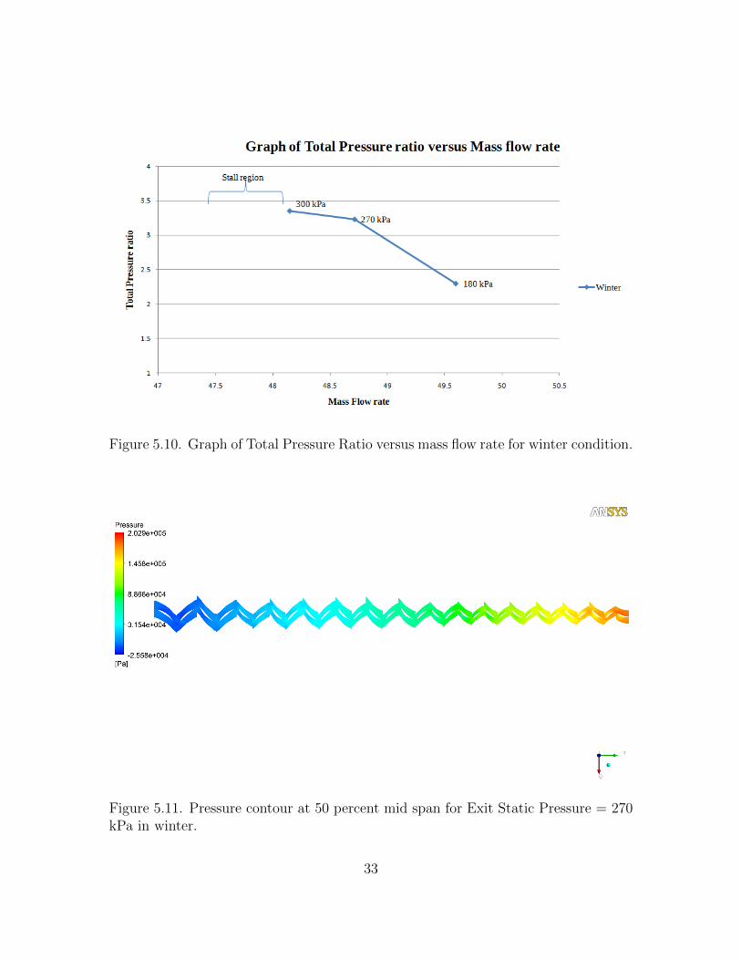
Figure 5.10. Graph of Total Pressure Ratio versus mass flow rate for winter condition.

Figure 5.11. Pressure contour at 50 percent mid span for Exit Static Pressure = 270kPa in winter.

33

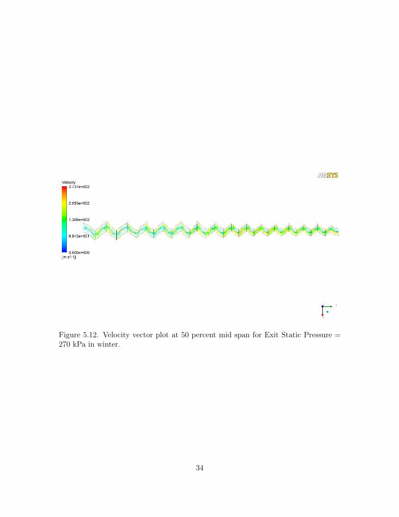
Figure 5.12. Velocity vector plot at 50 percent mid span for Exit Static Pressure =270 kPa in winter.

34

CHAPTER 6

Concluding Remarks

This research work presented the parameters that affect computational analysis

of a axial flow compressor and its performance. The research was carried out in two

segments:

• Preliminary analysis varying certain parameters

• Comparison of performance in two categories

The first segment started with two types of turbulence models, k-epsilon and

Shear Stress Transport and their effect on total pressure ratio and mass flow rate.

The use of Shear Stress Model showed a 10 percent increase in total pressure ratio.

Since SST model showed a notable variation in total pressure ratio for finer grids,

this model is concluded to be suitable for the present study. Once the turbulence

model is selected, a grid/y-plus sensitivity analysis is carried out by varying y-plus

from a value of 1 to 150 and number of nodes from 0.9 to 2 million. For each analysis,

wall clock time is observed in order to finalize perfect values, compromising certain

results.

Using SST as turbulence model and using a grid with y-plus value of 12 and 0.9

million nodes, a computational analysis is carried out for three climatic conditions

and three exit static pressures. The variation of stage total pressure ratio with stage

number for exit static pressure of 180 kPa for three climatic conditions is discussed.

Analysis using three exit static pressures 180, 270 and 300 kPa for winter condition

is graphically presented. The compressor stalling region is highlighted for further

improvement in compressor performance.

35

6.1 Future work

The results of the steady state analysis form base settings for the transient

analysis of the compressor. A transient analysis gives in depth knowledge on the

onset of flow seperation and flow transition between rotor and stator. The range of

compressor performance can be further increased by changing the stagger angles of

the stators in order to allow more mass flow rate at different climatic conditions.

36

APPENDIX A

INPUT CODE FOR PARALLEL PROCESSING

37

!/bin/csh

Batch file for running CFX jobs

start in the directory where the job was

submitted

-cwd

total number of nodes requested(each node has 4 processors)

-l qty.eq.9,quad

name of the job

-N s15ex

commands to be executed

call parallel CFX using ’paracfx’ script. Options can be added in quotes.

setenv PATH /usr/bin:PATH

rm -rf /tmp/*.dat /tmp/pvm*

time paracfx ” -solver-double -def 15 y12 s15.def ”

38

REFERENCES

[1] C. B. Meher-homji, “The Historical Evolution of Turbomachinery,” 2000.

[2] T. D. Canonsburg, “ANSYS CFX-Pre User ’ s Guide,” vol. 15317, no. October,

pp. 724–746, 2012.

[3] R. U. E. Ancelle, CFD Validation for Propulsion System Components ( la Vali-

dation CFD des organes des propdseurs ), 1998.

[4] MIT, “Multistage axial flow compressors.”

[5] Wikipedia, “Flynn’s taxonomy - Wikipedia, the free encyclopedia.”

[6] T. D. Canonsburg, “ANSYS CFX-Solver Theory Guide,” vol. 15317, no. October,

pp. 724–746, 2012.

[7] W. Chung-Hua, “ADVISORY COMMITTEE TECHNICAL NOTE 2302,” no.

March, 1951.

[8] J. D. Denton and W. N. Dawes, “Computational fluid dynamics for turboma-

chinery,” vol. 213, 1990.

[9] J. C. Tanhill, D. A. Anderson, and R. H. Pletcher, Computational Fluid Mechan-

ics And Heat Transfer - Anderson.pdf, 1997.

[10] T. Jiyuan, Y. Guan Heng, and L. Chaoqun, Computational Fluid Dynamics: A

Practical Approach. Butterworth-Heinemann, 2008.

[11] H. Chang, W. Zhao, D. Jin, Z. Peng, and X. Gui, “Numerical investigation

of base-setting of stators stagger angles for a 15-stage axial-flow compressor,”

Journal of Thermal Science, vol. 23, no. 1, pp. 36–44, Jan. 2014. [Online].

Available: http://link.springer.com/10.1007/s11630-014-0674-x

[12] D. D. Knight, “Parallel Computing in Computational Fluid Dynamics.”

39

[13] D. Roose and R. V. Driessche, “Parallel Computers and Parallel Algorithms for

CFD : An Introduction,” Tech. Rep.

[14] T. D. Canonsburg, “ANSYS TurboGrid User ’ s Guide,” vol. 15317, no. October,

pp. 724–746, 2012.

40

BIOGRAPHICAL STATEMENT

Chaithanya Mamidoju was born in the city of Nirmal, India in 1991. She ob-

tained a Bachelor’s degree in Aeronautical Engineering with a major in Aerodynamics

and Propulsion from Jawaharlal Nehru Technological University, Hyderabad in 2012.

After graduation she then came to the United States in Fall 2012 to pursue an M.S.

degree program in Aerospace Engineering at the University of Texas at Arlington.

Chaithanya has been a Tutor at the UTS for Student Support Services for Un-

dergraduate Students. Her research interests include Computational Fluid Dynamics,

Engineering Analysis and Design Optimization. She is currently working in the CFD

Lab with Dr. Brian Dennis. She is a student member of AIAA and SWE.

41