Computable General Equilibrium Models for the

Analysis of Energy and Climate Policies

Ian Sue Wing∗

Dept. of Geography and Environment, Boston University

Joint Program on the Science and Policy of Global Change, MIT

Prepared for the International Handbook of Energy Economics

Abstract

This chapter is a simple, rigorous, practically-oriented exposition of computable general

equilibrium (CGE) modeling. The general algebraic framework of a CGE model is developed

from microeconomic fundamentals, and employed to illustrate (i) how a model may be cali-

brated using the economic data in a social accounting matrix, (ii) how the resulting system of

numerical equations may be solved for the equilibrium values of economic variables, and (iii)

how perturbing this equilibrium by introducing price or quantity distortions facilitates analysis

of the economy-wide impacts of energy and climate policies.

JEL Classification: C68, D58, H22, Q43

Keywords : general equilibrium, CGE models, policy analysis, taxation

∗Rm. 461, 675 Commonwealth Ave., Boston MA 02215. Phone: (617) 353-5741. Email: isw@bu.edu. I amindebted to the U.S. Department of Energy Office of Science (BER) for support under grants DE-FG02-02ER63484and DE-FG02-06ER64204.

1

1 Introduction

Walrasian general equilibrium prevails when supply and demand are equalized across all of the

interconnected markets in the economy. Computable general equilibrium (CGE) models are sim-

ulations that combine the abstract general equilibrium structure formalized by Arrow and Debreu

with realistic economic data to solve numerically for the levels of supply, demand and price that

support equilibrium across a specified set of markets.

CGE models have emerged as a standard pseudo-empirical tool for policy evaluation. Their

strength lies in their ability to prospectively elucidate the character and magnitude of the economic

impacts of energy and environmental policies. Perhaps the most important of these applications is

the analysis of measures to reduce greenhouses gas (GHG) emissions—principally carbon dioxide

(CO2) from the combustion of fossil fuels. In the decade since the survey by Bhattacharyya (1996)

there has been an explosion in this literature on this topic, with over 150 articles in peer-reviewed

books and journals and an even greater number of working papers and technical reports. GHG

mitigation policies can incorporate a range of instruments ranging from taxes and subsidies to

income transfer schemes to quotas on the carbon content of energy goods. The fact that energy

is an input to virtually every economic activity, coupled with the limited possibilities to substitute

other commodities for fossil fuels, imply that these policies’ effects will ripple through multiple

markets, with far larger consequences than energy’s small share of national income might suggest.

This phenomenon is the central motivation for the general equilibrium approach.

But, notwithstanding their popularity, CGE models continue to be viewed in some quarters

as a “black box”, whose complex internal workings obfuscate the linkages between their outputs

and features of their input data, algebraic structure, or method of solution, and worse, allow ques-

tionable assumptions to be hidden within them that end up driving their results.1 This chapter

addresses this presumption by opening up the black box to scrutiny, elucidating the simple alge-

braic framework shared by all CGE models (regardless of their size or apparent complexity), the

2

key features of their data base and the calibration methods used to incorporate this information into

their algebraic framework, and the numerical techniques used to solve the resulting mathematical

programming problem.

To accomplish all this in a single article it will be necessary to move beyond a traditional

survey of the modeling literature, which is necessarily broad, and of which many examples have

recently been published (e.g., Conrad, 1999, 2001; Bergman, 2005). I take the different approach

of concisely synthesizing material which is usually spread across a broad cross-section of the

energy economics, policy and modeling literatures.2 Taking a cue from earlier work (Shoven and

Whalley, 1984; Kehoe and Kehoe, 1995; Kehoe, 1998a) I employ the microeconomic foundations

of consumer and producer maximization to develop a framework that both straightforward and

sufficiently general to represent a CGE model of arbitrary size and dimension. This framework

is then used to demonstrate in a practical fashion how a social accounting matrix may be used to

calibrate the coefficients of the model equations, how the resulting system of numerical equations

is solved, and how the equilibrium thus solved for may be perturbed and the results used to analyze

the economic effects of various types of energy policies. The result is a transparent and systematic,

yet also theoretically coherent and reasonably comprehensive, introduction to the subject of CGE

modeling.

The plan of the chapter is as follows. Section 2 introduces the circular flow of the economy, and

demonstrates how it serves as the fundamental conceptual starting point for Walrasian equilibrium

theory that underlies a CGE model. Section 3 presents a social accounting matrix and illustrates

how the algebra of its accounting rules reflects the conditions of general equilibrium. Section 4

develops these relationships into a workable CGE model using the device of the constant elasticity

of substitution (CES) economy in which households have CES preferences and firms have CES

production technology. Section 5 uses the CES economy to illustrate how models are numerically

calibrated, while 6 discusses issues which arise in solving CGE models. Section 7 explains how

CGE models are used to analyze energy and climate policies. An application is presented in section

3

8, in which the CES economy is employed to elucidate the impact of limiting CO2 emissions in

the U.S. Section 9 offers a brief summary and concluding remarks.

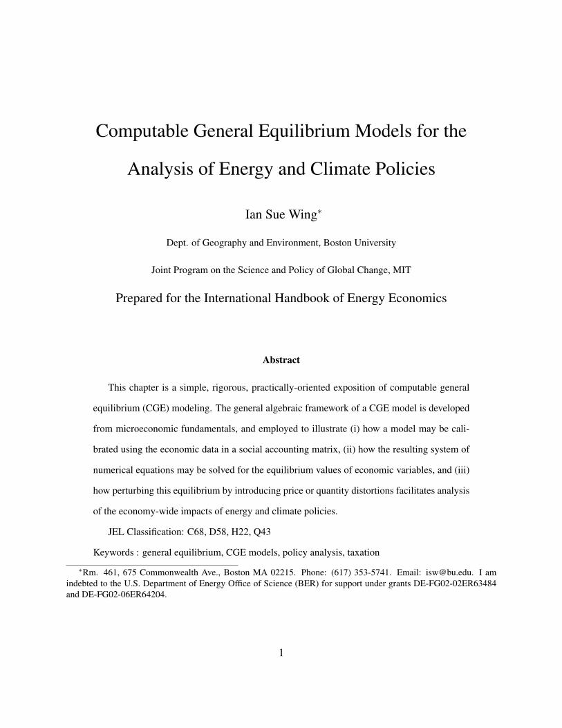
Figure 1: The Circular Flow

Government

Taxes Taxes

Goods & Services

Goods & Services

Factor Markets

Firms

Households

Expenditure

Profits/ Factor Income

Goods & Services

Factor Inputs

Product Markets

Payments Goods and factors

2 Foundations: The Circular Flow and Walrasian Equilibrium

The fundamental conceptual starting point for a CGE model is the circular flow of commodities in

a closed economy, shown in Figure 1. The main actors in the diagram are households, who own

the factors of production and are the final consumers of produced commodities, and firms, who

rent the factors of production from the households for the purpose of producing goods and services

that the households then consume. Many CGE models also explicitly represent the government,

4

but its role in the circular flow is often passive: to collect taxes and disburse these revenues to firms

and households as subsidies and lump-sum transfers, subject to rules of budgetary balance that are

specified by the analyst. In tracing the circular flow one can start with the supply of factor inputs

(e.g. labor and capital services) to the firms and continue to the supply of goods and services from

the firms to the households, who in turn control the supply of factor services. One may also begin

with payments, which households receive for the services of labor and capital provided to firms by

their primary factor endowment, and which are then used as income to pay producing sectors for

the goods and services that the households consume.

Equilibrium in the economic flows in Figure 1 results in the conservation of both product and

value. Conservation of product, which holds even when the economy is not in equilibrium, reflects

the physical principle of material balance that the quantity of a factor with which households are

endowed, or of a commodity that is produced by firms, must be completely absorbed by the firms or

households (respectively) in the rest of the economy. Conservation of value reflects the accounting

principle of budgetary balance that for each activity in the economy the value of expenditures

on inputs (i.e., price × quantity) must be balanced by the value of the income that it earns, and

that each unit of expenditure has to purchase some amount of some type of commodity. The

implication is that neither product nor value can appear out of nowhere: each activity’s production

or endowment must be matched by others’ uses, and each activity’s income must be balanced by

others’ expenditures. Nor can product or value disappear: a transfer of purchasing power can

only be effected through an opposing transfer of some positive amount of some produced good or

primary factor service, and vice versa.

These accounting rules are the cornerstones of Walrasian general equilibrium. Conservation of

product, by ensuring that the flows of goods and factors must be absorbed by the production and

consumption activities in the economy, is an expression of the principle of no free disposability. It

implies that firms’ outputs are fully consumed by households, and that households’ endowment of

primary factors is in turn fully employed by firms. Thus, for a given commodity the quantity pro-

5

duced must equal the sum of the quantities of that are demanded by the other firms and households

in the economy. Analogously, for a given factor the quantities demanded by firms must completely

exhaust the aggregate supply endowed to the households. This is the familiar condition of market

clearance.

Conservation of value implies that the sum total of revenue from the production of goods must

be allocated either to households as receipts for primary factors rentals, to other industries as pay-

ments for intermediate inputs, or to the government as taxes. The value of a unit of each commodity

in the economy must then equal the sum of the values of all the inputs used to produce it: the cost

of the inputs of intermediate materials as well as the payments to the primary factors employed

in its production. The principle of conservation of value thus simultaneously reflects constancy of

returns to scale in production and perfectly competitive markets for produced commodities. These

conditions imply that in equilibrium producers make zero profit.3

Lastly, the returns to households’ endowments of primary factors, which are the value of their

factor rentals to producers, constitute income which the households exhaust on goods purchases.

The fact that households’ factor endowments are fully employed, so that no amount of any factor

is left idle, and that households exhaust their income, purchasing some amount of commodities—

even for the purpose of saving, reflects the principle of balanced-budget accounting known as

income balance. One can also think of this principle as a zero profit condition on the production

of a “utility good”, whose quantity is given by the aggregate value of households’ expenditures

on commodities, and whose price is the marginal utility of aggregate consumption, or the unit

expenditure index.

As I go on to demonstrate, CGE models employ the market clearance, zero profit and income

balance conditions to solve simultaneously for the set of prices and the allocation of goods and

factors that support general equilibrium. Walrasian equilibrium is defined not by the transaction

processes through which this allocation comes about, but by the allocation itself, which is made

up of the components of the circular flow shown by solid lines in Figure 1. General equilibrium is

6

therefore customarily modeled in terms of barter trade in commodities and factors, without the need

to explicitly keep track of (or even represent) the compensating financial transfers. Consequently,

it is rare for CGE models to explicitly include money as a commodity. Nevertheless, the relative

values of the different commodities and factors still need to be made denominated using some

common unit of account. This is accomplished by expressing the simulated flows in terms of the

value of one commodity (the so-called numeraire good) whose price is fixed. For this reason, CGE

models only solve for relative prices. I expand on this point in Section 4.

3 The Algebra of Equilibrium and the Social Accounting Ma-

trix

We now outline the algebraic expression of the circular flow, and its use in tabulating the economic

data on which CGE models are calibrated. Consider a hypothetical closed economy made up of

N industries, each of which produces its own type of commodity, and an unspecified number

of households that jointly own an endowment of F different types of primary factors. Three

key assumptions about this economy simplify the analysis which follows. First, there are no tax

or subsidy distortions, or quantitative restrictions on transactions. Second, the households act

collectively as a single representative agent who rents out the factors to the industries in exchange

for income. Households then spend the latter to purchase the N commodities for the purpose

of satisfying D types of demands (e.g., demands for goods for the purposes of consumption and

investment). Third, each industry behaves as a representative firm that hires inputs of the F primary

factors and uses quantities of theN commodities as intermediate inputs to produce a quantity y of

its own type of output.

I use the indices i = {1, . . . , N} to indicate the set of commodities, j = {1, . . . ,N} to in-

dicate the set of industry sectors, f = {1, . . . ,F} to indicate the set of primary factors, and

7

d = {1, . . . ,D} to indicate the set of final demands. The circular flow of the economy can be

completely characterized by three data matrices: anN ×N input-output matrix of industries’ uses

of commodities as intermediate inputs, X, an F ×N matrix of primary factor inputs to industries,

V, and an N ×D matrix of commodity uses by final demand activities, G.

It is straightforward to establish how the elements of the three matrices may be arranged to

reflect the logic of the circular flow. First, commodity market clearance implies that the value of

gross output of industry i, which is the value of the aggregate supply of the ith commodity (yi)

must equal the sum of the values of the j intermediate uses (xi,j) and the d final demands (gi,d)

which absorb that commodity:

yi =N∑j=1

xi,j +D∑d=1

gi,d (1)

Similarly, factor market clearance implies that the sum of firms’ individual uses of each primary

factor (vf,j) fully utilize the representative agent’s corresponding endowment (V f ):

V f =N∑j=1

vf,j (2)

Second, the fact that industries make zero profit implies that the value of gross output of the j th

sector (yj) must equal the sum of the benchmark values of inputs of the i intermediate goods, xi,j ,

and f primary factors, vf,j , employed by that industry’s production process:

yj =N∑i=1

xi,j +F∑f=1

vfj (3)

Third, the representative agent’s income, I, is made up of the receipts from the rental of primary

factors—all of which are assumed to be fully employed. The resulting income must balance the

agent’s gross expenditure on satisfaction of commodity demands. Together, these conditions imply

that income is equivalent to the sum of the elements of V, which in turn must equal the sum of the

8

Figure 2: A Social Accounting Matrix

← j → ← d → Row Total1 . . . N 1 . . . D

↑ 1 y1

i... X G

...↓ N yN

↑ 1 V 1

f... V

...↓ F V F

ColumnTotal y1 . . . yN G1 . . . GD

elements of G. Thus, by eq. (2),

I =F∑f=1

V f =N∑i=1

D∑d=1

gid (4)

The accounting relationships in eqs. (1)-(4) jointly imply that, in order to reflect the logic of the

circular flow, the matrices X, V and G should be arranged according to Figure 2(a). This diagram

is an accounting tableau known as a social accounting matrix (SAM), which is a snapshot of the

inter-industry and inter-activity flows of value within an economy at equilibrium in a particular

benchmark period. The SAM is an array of input-output accounts that are denominated in the units

of value of the period for which the flows in the economy are recorded, typically the currency of

the benchmark year. Each account is represented by a row and a column, and the cell elements

record the payment from the account of a column to the account of a row. Thus, an account’s

components of income of (i.e., the value of receipts from the sale of a commodity) appear along

its row, and the components of its expenditure (i.e., the values of the inputs to a demand activity or

the production of a good) appear along its column (King 1985).

The structure the SAM reflects the principle of double-entry book-keeping, which requires that

9

for each account, total revenue-the row total-must equal total expenditure-the column total. This

is apparent from Figure fig:sam(a), where the sum across any row in the upper quadrants X and

G is equivalent to the expression for goods market clearance from eq. (1), and the sum across any

row in the south-west quadrant V is equivalent to the expressions for factor market clearance from

eq. (2). Likewise, the sum down any column of the left-hand quadrants X and V is equivalent to

the expression for zero-profit in industries from eq. (3). Furthermore, once these conditions hold,

the sums of the elements of the northeast and southwest quadrants (G and V, respectively) should

equal one another, which is equivalent to the income balance relationship from eq. (4). The latter

simply reflects the intuition that in a closed economy GDP (the aggregate of the components of

expenditure) is equal to value added (the aggregate of the components of income). These properties

make the SAM an ideal data base from which to construct a CGE model.

4 From a SAM to a CGE Model: The CES Economy

CGE models’ algebraic framework results from the imposition of the axioms of producer and

consumer maximization on the accounting framework of the SAM. To illustrate this point I use

the pedagogic device of a constant elasticity of substitution (CES) economy in which households

are treated as a representative agent with CES preferences and industry sectors are modeled as

representative producers with CES production technologies. While the algebra thus far has all been

developed in terms of flows of value, in the subsequent analysis it will be necessary to distinguish

between the prices and quantities of goods and factors. I therefore use pi and wf to denote the

prices of commodities and factors, respectively, and use xi,j , vf,j and gi,d (i.e., without bars) to

indicate the quantity components of the previously-defined value variables.

10

4.1 Households

The objective of the representative agent is to maximize utility (u) by choosing levels of goods

consumption (gi,C), subject to ruling commodity prices (pi) and the agent’s budget constraint.

The agent may also demand goods and services for purposes other than consumption (C). In

the present example, I assume that d = {C,O}, where O indicates other final demands (e.g., sav-

ing/investment) which are given by the exogenous vector gi,O. Using eq. (4), the agent’s disposable

income is then:

µ =F∑f=1

wfVf −N∑i=1

pigi,O, (5)

which allows us to specify the agent’s problem as:

maxgi,C

u[g1,C , . . . , gN ,C ] s.t. µ =N∑i=1

pigi,C . (6)

We assume that the representative agent has CES preferences, so that her utility function is

u =

(N∑i=1

αig(ω−1)/ωi,C

)ω/(ω−1)

,

where the αis are the technical coefficients of the utility function, and ω is the elasticity of substi-

tution.

Rather than solve (6) directly, it is advantageous to solve the dual expenditure minimization

problem. The agent therefore seeks to minimize her expenditure to gain a unit of utility (θ), subject

to the constraint of her utility function by choosing the levels of unit commodity demands, (gi,C):

mingi,C

θ =N∑i=1

pigi,C s.t. 1 =

(N∑i=1

αig(ω−1)/ωi,C

)ω/(ω−1)

. (6′)

The variable θ is known as the unit expenditure index, and can be interpreted as the marginal

11

utility of aggregate consumption. The solution to this problem is the vector of unit demands for

the consumption of commodities (gi,C = αωi θωp−ωi ), which implies the conditional final demands:

gi,C = gi,Cu = αωi θωp−ωi u, (7)

where u indicates the representative agent’s level of activity.

4.2 Producers

Each producer maximizes profit (πj) by choosing levels of intermediate inputs (xi,j) and primary

factors (vf,j) to produce output (yj), subject to the ruling prices of output (pj) intermediate inputs

(pi), factors (wf ) and the constraint of its production technology (ϑj). The j th producer’s problem

is thus:

maxxi,j , vf,j

πj = pjyj −N∑i=1

pixi,j +F∑f=1

wfvf,j s.t. yj = ϑj[x1,j, . . . , xN ,j; v1,j, . . . , vF ,j] (8)

Producers have CES technology, so that the production function ϑj takes the form

yj =

(N∑i=1

βi,jx(σj−1)/σj

i,j +F∑f=1

γf,jv(σj−1)/σj

f,j

)σj/(σj−1)

,

where, βi,j and γi,j are the technical coefficients on intermediate commodities and primary factors

respectively, while σj denotes each industry’s elasticity of substitution.

Instead of solving (8) directly, it will prove useful to solve the dual cost minimization problem.

Firm j seeks to minimize its unit cost subject to the constraint of its production technology by

12

choosing the levels of the unit input demands for commodities (xi,j) and the primary factor (vf,j):

minxi,j , vf,j

pj =N∑i=1

pixi,j+F∑f=1

wf vf,j s.t. 1 =

(N∑i=1

βi,jx(σj−1)/σj

i,j +F∑f=1

γf,j v(σj−1)/σj

f,j

)σj/(σj−1)

(8′)

The solution to this problem yields the unit demands for inputs of intermediate commodities and

primary factors (xi,j = βσj

i,jpσj

j p−σj

i and vh,j = γσj

f,jpσj

j w−σj

f ), which imply the conditional input

demands:

xi,j = xi,jyj = βσj

i,jpσj

j p−σj

i yj, , (9)

vf,j = vf,jyj = γσj

f,jpσj

j w−σj

f yj, (10)

where yj indicates producers’ activity levels.

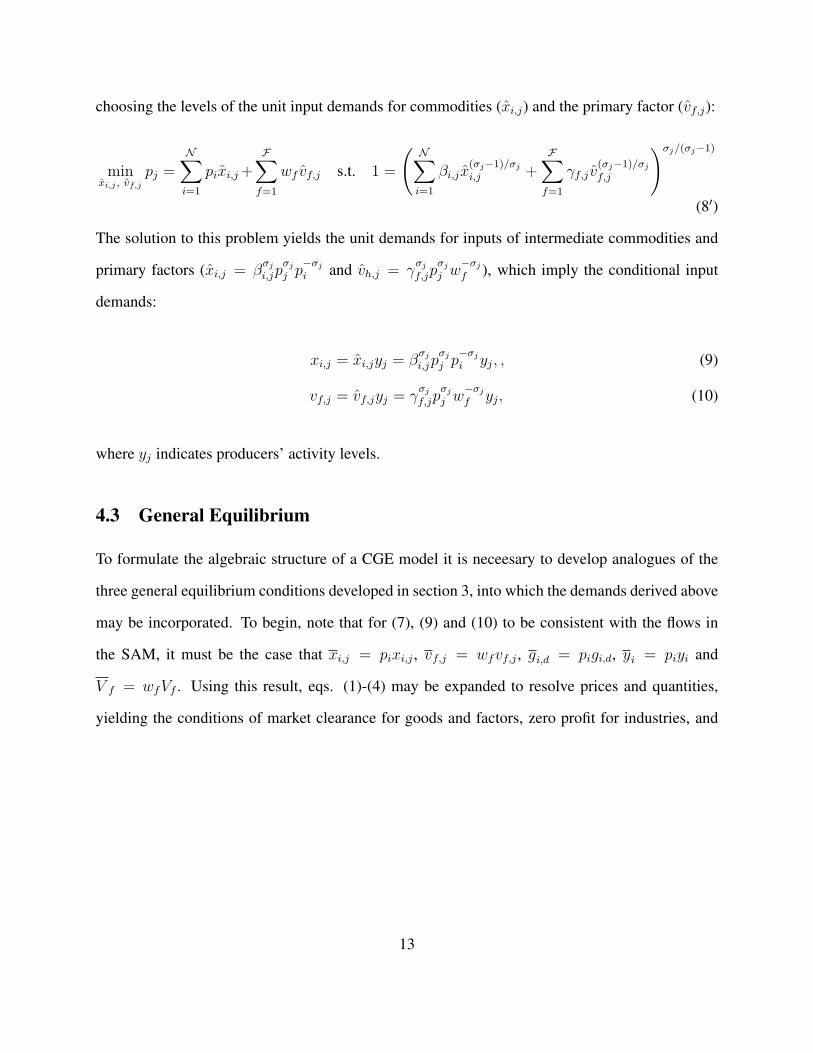
4.3 General Equilibrium

To formulate the algebraic structure of a CGE model it is neceesary to develop analogues of the

three general equilibrium conditions developed in section 3, into which the demands derived above

may be incorporated. To begin, note that for (7), (9) and (10) to be consistent with the flows in

the SAM, it must be the case that xi,j = pixi,j , vf,j = wfvf,j , gi,d = pigi,d, yi = piyi and

V f = wfVf . Using this result, eqs. (1)-(4) may be expanded to resolve prices and quantities,

yielding the conditions of market clearance for goods and factors, zero profit for industries, and

13

income balance for the representative agent:

piyi = pi

(N∑j=1

xi,j + gi,C + gi,O

), (1′)

wVf = wN∑j=1

vf,j, (2′)

pjyj =N∑i=1

pixi,jyj +F∑f=1

wf vf,jyj, (3′)

µ =F∑f=1

wfVf −N∑i=1

pigi,O =N∑i=1

pigi,Cu = θu. (4′)

A crucial insight, due to Mathiesen (1985a,b), is that eqs. (1′)-(4′) are analogous to the Karush-

Kuhn-Tucker conditions for the optimal allocation of commodities and factors and the distribution

of activities in the economy.4 In particular, the variable which is the common factor in each of the

foregoing equations exhibits complementary slackness with respect to the corresponding residual

primal or dual constraint. Far from being a mere technical detail, this characteristic is what has

revolutionized the formulation and solution of CGE models.

The economic intuition behind complementary slackness is straightforward. In (3′), any pro-

ducer earning negative profit will shut down with an output of zero; accordingly, the expression

for unit profit is complementary to the relevant producer’s level of activity (yj). The constraint

qualification may therefore be written:

pj <N∑i=1

pixi,j +F∑f=1

wf vf,j, yj = 0 or pj =N∑i=1

pixi,j +F∑f=1

wf vf,j, yj > 0 (11)

An additional insight is that similar logic applies to the representative agent, whose optimal con-

sumption decision can be thought of as zero profit in the “production” of utility: if the cost of the

goods necessary to generate a unit of final consumption exceeds the latter’s marginal utility, then

14

there will be no consumption activity. The extreme right-hand equality in (4′) therefore implies:

θ <N∑i=1

pigi,C , u = 0 or θ =N∑i=1

pigi,C , u > 0 (12)

In (1′) and (2′), any commodity or factor which is in excess supply will have a price of zero;

therefore the balance between supply and demand for each of these inputs is complementary to the

corresponding price level (pj and wf , respectively).

yi >N∑j=1

xi,j + gi,C + gi,O, pi = 0 or yi =N∑j=1

xi,j + gi,C + gi,O, pi > 0 (13)

Vf >N∑j=1

vf,j, wf = 0 or Vf =N∑j=1

vf,j, wf > 0 (14)

The incorporation of utility as a good within the equilibrium framework permits the specification

of a market clearance condition for u, which states that a supply of utility in excess of that provided

by consumption results in zero unit expenditure:

u > µ/θ, θ = 0, or u = µ/θ, θ ≥ 0 (15)

Finally, it is worth noting that the definition of disposable income, which is restated as the

extreme left-hand equality in (4′), does not exhibit complementary slackness with respect to any of

its constituent variables, and moreover is made redundant by (15). In the specification of general

equilibrium it plays the simple role of an accounting identity. One way to make this role explicit is

to designate the unit expenditure index as the numeraire price by fixing θ = 1. This automatically

drops eq. (15) by fixing µ = u.

15

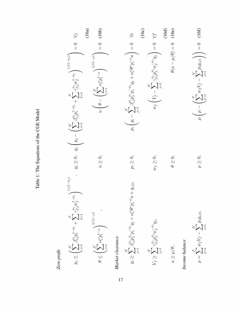
4.4 The CGE model in a Complementarity Format

The specification of a CGE model in a complementarity format involves pairing each of the ex-

pressions (11)-(15) with the associated complementary variable so as to make complementarity

explicit (Rutherford, 1995). Using (7), (9) and (10) to make the appropriate substitutions yields

the algebraic system (16a)-(16f) shown in Table 1. These equations are what is referred to as “a

CGE model”.

This system defines the pseudo-excess demand correspondence of the economy:

Ξ(z) ≥ 0, z ≥ 0, z′Ξ(z) = 0, (16)

where Ξ = {p, θ,y,V , u,m}′ is the stacked vector of 2N+F+3 equations and z = {y, u,p,w, θ,m}

is the 2N + F + 3-vector of unknowns:5

1. N + 1 zero profit inequalities {p, θ} in as many unknowns {y, u},

2. N + F + 1 market clearance inequalities {y,V , u} as many unknowns {p,w, θ}, and

3. A single income definition equation (µ) in a single unknown (µ).

Henceforth I use the shorthand notation “⊥” to denote the complementary slackness relationship

exhibited by the model’s equations and its associated variables, writing (16) compactly as:

Ξ(z) ≥ 0, ⊥ z.

Note that in equilibrium the equations in the rightmost column of Table 1 will all be satisfied with

equality, while the variables in the middle column will all be positive.

16

Tabl

e1:

The

Equ

atio

nsof

the

CG

EM

odel

Zero

profi

t

p j≤

( N ∑ i=1

βσ

j

i,jp1−σ

j

i+

F ∑ f=

1

γσ

j

f,jw

1−σ

j

f

) 1/(1−σ

j)

,y j≥

0,y j

p j−

( N ∑ i=1

βσ

j

i,jp1−σ

j

i+

F ∑ f=

1

γσ

j

f,jw

1−σ

j

f

) 1/(1−σ

j) =

0∀j (1

6a)

θ≤

( N ∑ i=1

αω ip1−ω

i

) 1/(1−ω)

,u≥

0,u

θ−( N ∑ i=

1

αω ip1−ω

i

) 1/(1−ω) =

0(1

6b)

Mar

ketc

lear

ance

y i≥

N ∑ j=1

βσ

j

i,jpσ

j

jp−

σj

iy j

+αω iθωp−

ωiu

+g i,O,

p i≥

0,p i

( y i−

N ∑ j=1

βσ

j

i,jpσ

j

jp−

σj

iy j

+αω iθωp−

ωiu

) =0∀i (1

6c)

Vf≥

N ∑ j=1

γσ

j

f,jpσ

j

jw−σ

j

fy j,

wf≥

0,wf

( Vf−

N ∑ j=1

γσ

j

f,jpσ

j

jw−σ

j

fy j

) =0∀f (1

6d)

u≥µ/θ,

θ≥

0,θ(u−µ/θ

)=

0(1

6e)

Inco

me

bala

nce

µ=

F ∑ f=

1

wfVf−

N ∑ i=1

p ig i,O,

µ≥

0,µ

( µ−

( F ∑ f=

1

wfVf−

N ∑ i=1

p ig i,O

)) =0

(16f

)

17

5 Numerical Calibration

The problem in eq. (16) is highly non-linear, with the result that a closed-form solution for z

does not exist. This is the reason for the “C” in CGE models: to find the general equilibrium of

an economy with realistic utility and production functions, the corresponding system of equations

must be calibrated on a SAM introduced in section 3 to generate a numerical problem that can be

solved using optimization techniques.

To numerically calibrate our example CES economy, we need to establish equivalence between

eqs. (1)-(4) and (1′)-(4′). There are different ways of doing this, depending on what kind of infor-

mation is available in addition to the SAM. Most frequently however, data on benchmark prices are

lacking.6 In this situation the simplest method to “fit” eq. (16) to the benchmark equilibrium in the

SAM is to treat the price variables as indices with benchmark values of unity: pi = wf = θ = 1,

and treat the activity and income variables as real values which are set equal to the row and column

totals in the SAM: xi,j = xi,j , vf,j = vf,j , gi,d = gi,d, yi = yi, Vf = V f , u = µ = GC . Then, the

technical coefficients of the cost and expenditure equations may be computed by substituting these

conditions into the demand functions (7), (9) and (10):

αi,C =(gi,C/GC

)1/ω, βi,j =

(xi,j/yj

)1/σj and γf,j =(vf,j/yj

)1/σj . (17)

This result is essentially the same as the “calibrated share form” of of CES function (see, e.g.,

Böhringer et al., 2003).

Inserting the foregoing calibrated parameters into the expressions in Table 1, along with values

for the elasticities of substitution σ and ω specified by the analyst, generates a system of numerical

inequalities in which constitutes the actual CGE model. It is particularly important to realize that

to satisfy the resulting expressions with equality, one simply has to set the price variables equal

to unity and the quantity variables equal to the corresponding values in the SAM. This procedure,

18

known as benchmark replication, permits the analyst to verify that the calibration is correct. The

intuition is that since a balanced SAM represents the initial equilibrium of the model, plugging

the values in the SAM back into the calibrated numerical pseudo-excess demand correspondence

should yield an equilibrium.

Note that (17) allows us to replace the terms αωi,C , βσj

i,j and γσj

f,j in eq. (16) with coefficients

given by the ratio of the relevant cells of the SAM and the corresponding column totals. The

key implication is that the values of the substitution elasticities have no practical impact on the

benchmark equilibrium, which makes intuitive sense because the model’s initial equilibrium is de-

termined by SAM, and is therefore consistent with an infinite number of potential values for σ and

ω. The corollary is that the substitution possibilities in the economy—i.e., the degree of adjustment

of economic quantities in response to changes in prices, both within and between sectors—are fun-

damentally determined by the SAM.

Figure 3: Calibration, the Elasticity of Substitution, and Adjustment to Price Changes E / Y σL Isoquant

/E Y′

σH Isoquant

A

A′

B

B′

P

/E Y

M / Y /M Y P ′M Y/

19

A simple example clarifies this point. Figure 3 illustrates the intra-industry margin of substi-

tution for a hypothetical industry that produces output, Y , from inputs of energy, E and materials,

M . Benchmark data on the values of the inputs (E andM ) and output (Y = E+M ), together with

the assumption of unitary prices (given by the −45◦ line PP ), define a unique calibration point:

A. An infinite number of potential isoquants pass through this point, so to pin down the industry’s

specific technology it is necessary to make an assumption about the elasticity of substitution (σ).

A low or a high value for this parameter (σL or σH) makes the isoquant more or less highly curved,

thus admitting a smaller or larger adjustment in input intensities in response to a given rotation of

the relative price line, A→ B. The locus of the calibration point is equally important for this pro-

cess: starting from another benchmark input distribution, A′ (where Y = E′+M

′), the difference

between the new pattern of adjustment (A′ → B′) and the original is easily as large as the shift

induced by a change in σ.

This discussion raises the question of how precisely to determine the elasticity of substitution,

which turns out to be a thorny issue. In our simple CES economy there are more free parameters

than there are model equations or observations of benchmark data, which makes (17) an under-

determined mathematical problem. This difficulty is magnified in real-world CGE models, in

which it has become popular to specify industries’ cost and consumers’ expenditure functions

using hierarchical CES functions, each of which has multiple elasticities of substitution.

The nested production and cost functions in the Goulder (1995) model are shown in Figure 4,

in which each node of the tree denotes the output of a CES function and the branches denote the

relevant inputs. In each industry, the substitution possibilities among capital (K), labor (L), energy

(E) and materials (M ) are controlled by five elasticity parameters: substitution between primary

factors (KL) and intermediate goods (EM ) by σO, capital-labor substitution by σKL, energy-

material substitution by σEM , inter-fuel substitution by σE , and substitution among non-energy

intermediate inputs by σM .

It is not possible to either estimate or compute the values of these elasticities without a host

20

Figure 4: Goulder (1995) KLEM Production Structure

qO

σE

σKLEM

σM

qKL qEM

qM

σEM

qE

qK qL

σKL ← X

mq → ← q → Xe

pO

σE

σKLEM

σM

pKL pEM

pM

σEM

pE

pK pL

σKL ← X

mp → ← Xep →

qO

σE

σKLEM

σM

qKL qEM

qM

σEM

qE

qK qL

σKL ← X

mq → ← q → Xe

pO

σE

σKLEM

σM

pKL pEM

pM

σEM

pE

pK pL

σKL ← X

mp → ← Xep →

A. Production B. Cost

Notes: pO, qO = price and quantity of output; P = {pK , pL, pE , pM}, Q = {qK , qL, qE , qM} = price and quantityof capital, labor, energy and materials; pX

e , qXe = price and quantity of intermediate energy commodities; pX

m, qXm =

price and quantity of intermediate material commodities; pKL, qKL = price and quantity of value-added composite;pEM , pEM = price and quantity of energy-materials composite.

of auxiliary information.7 Faced with this data constraint, modelers frequently resort to selecting

values for these parameters from the empirical literature based on judgment and assumptions.

The ad-hoc nature of this process has been criticized by mainstream empirical economists (e.g.,

Jorgenson, 1984; McKitrick, 1998), who advocate an econometric approach to CGE modeling in

which the pseudo-excess demand correspondence is built up from statistically estimated cost and

expenditure functions.

The econometric approach remedies the problematic inconsistency between the nested CES

functional forms employed in models and the flexible power series approximations of arbitrary cost

or expenditure functions employed by empirical studies, which estimate the pairwise Allen-Uzawa

elasticities of substitution (AUES) among the various inputs to production and consumption. For

example, the Translog form of the cost function in Figure 4 might specify the logarithm of the

21

output price as a quadratic function of the logarithms of the input prices (P) and time (t):

log pO = δ0 + δP log P′ + δT t+ 12log Pδ′PP log P + δPT log P′t+ 1

2δTT t

2, (18)

where δ0, δT , δTT , δP , δPP , and δPT are vectors of parameters to be estimated. By Shepard’s

Lemma, the derivative of this expression with respect to the logarithms of the input prices yields a

vector of input cost shares, s = {sK , sL, sE, sM}:

∂ log pO

∂ log P′ =diag(PQ′)

pOqO= s′ = δ′P + log PδPP + δ′PT t, (19)

where Q is the vector of input quantities.

Estimating (18) and (19) as a system yields a vector of numerically calibrated linear equations

which may be used in our example model as an alternative to eq. (17). We would need to substitute

(18) in place of the CES cost function (16a), and substitute commodity and factor demands derived

from (19) into the market clearance conditions (16c) and (16d). Substitution possibilities would

then be determined by the AUES between each pair of inputs k and l: ζkl = 1+ δkl/(sksl

), where

s indicates the mean value of each input’s share of total cost in the data sample. Note that our

original assumption of CES technology implies that ζKL,j = ζKE,j = ζKM,j = ζLE,j = ζLM,j =

ζEM,j = σj , which is a stringent restriction on the estimated parameters. Dawkins et al. (2001)

provide an excellent survey of these issues.

Despite its rigor, this approach is not without drawbacks. First and foremost, it is data intensive,

requiring time series observations of prices and quantities of the inputs and outputs for every

industry represented in the CGE model. Oftentimes such data are simply not available, which

has sharply limited its appeal.8 A second, more subtle shortcoming involves flexible functional

forms themselves. For the general equilibrium condition of no free disposability to be satisfied,

the simulated cost shares must be strictly positive at all prices. But it has long been known (e.g.,

22

Lutton and LeBlanc (1984)) that large and negative estimated values of δPP can give rise to cost

shares which are negative! For this reason, Perroni and Rutherford (1998) argue that flexible

functional forms lack global regularity, in the sense that (18) or (19) are not guaranteed to map an

arbitrary vector of positive prices into R+. In practice, it is not possible to predict a priori when

such problems will arise, and in any case, modelers have come up with ad-hoc countermeasures.9

Nevertheless, this remains remains an important issue for energy and climate policy simulations,

as the imposition of a sufficiently high tax on energy (say) may cause pE to increase outside of the

historical range of values, with the result that sE < 0 if the own- or cross-price energy elasticities

are sufficiently large.

6 Computation of Equilibrium

6.1 Solution Algorithms: A Sketch

The calibration procedure transforms (16) into a square system of numerical inequalities known as

a mixed complementarity problem or MCP (Ferris and Pang, 1997), which may be solved using

algorithms that are now routinely embodied in modern, commercially-available software systems

for optimization. Mathiesen (1985a,b) and Rutherford (1987) describe the basic approach, which

is essentially a Newton-type algorithm. The algorithm iteratively solves a sequence of linear com-

plementarity problems or LCPs (Cottle et al., 1992), each of which is a first-order Taylor series

expansion of the non-linear function Ξ. The LCP solved at each iteration is thus one of finding

z ≥ 0 s.t. ξ1 + ξ2z ≥ 0, zT (ξ1 + ξ2z) = 0 (20)

where, linearizing Ξ around z{ι}, the state vector of prices, activity levels and income at iteration

ι, ξ1[z{ι}] = ∇Ξ[z{ι}]z{ι} − Ξ[z{ι}] and ξ2[z{ι}] = ∇Ξ[z{ι}]. The value of z that solves the sub-

problem (20) at the ιth iteration is z?{ι}. Then, starting from an initial point, z{0}, the algorithm

23

generates a sequence of vectors z which is propagated according to the linesearch:

z{ι+1} = λ{ι}z?{ι} + (1− λ{ι})z{ι−1} (21)

where the parameter λ{ι} controls the length of the forward step at each iteration. The conver-

gence criterion for the algorithm made up of eqs. (20) and (21) is ‖Ξ(z?)‖ < ϕ, the maximum

level of excess demand, profit or income at which the economy is deemed by the analyst to have

attained equilibrium. The operations research literature now contains numerous refinements to

this approach, based on path-following homotopy methods described in Kehoe (1991, pp. 2061-

2065) and Eaves and Schmedders (1999).10 In modern software implementations, ϕ is routinely

six orders of magnitude smaller than the value of aggregate income.

6.2 A Digression on the Existence and Uniqueness of Equilibrium

The foregoing exposition raises the question of how good are CGE models at finding an equilib-

rium. Experience with the routine use of CGE models calibrated on real-world economic data to

solve for equilibria with a variety of price and quantity distortions would seem to indicate that the

procedures outlined above are robust. However, an answer to this question is both involved and

elusive, as it hinges on three important underlying issues which span the theoretical and empirical

literatures on general equilibrium: the existence, uniqueness, and stability of equilibrium. Clearly,

these are desirable attributes of a CGE model, as they imply that its solutions are both deterministic

and robust to perturbations along the path to equilibrium (i.e., as λ{ι} changes).

Textbook treatments of the theory of general equilibrium emphasize two properties that Ξ

should satisfy. The first is the weak axiom of revealed preference (WARP), whereby an economy

with multiple households exhibits a stable preference ordering over consumption bundles in the

space of all possible prices and income levels, ruling out the potential for non-homothetic shifts

in households’ consumption vectors due to changes in the distribution of income with prices held

24

constant. A sufficient condition for this property to hold is that households’ preferences admit

aggregation up to well-behaved community utility function, which is the representative agent as-

sumption. The second property is gross substitutability (GS), where the aggregate demand for any

commodity or factor is non-decreasing in the prices of all other goods and factors. Where this

condition holds, a vector of equilibrium prices exists and is unique up to scalar multiple (Varian,

1992).

One can think of these properties as economic interpretations of the sufficient conditions for

a unique solution to (16). From a mathematical standpoint, a (locally) unique solution for z can

be recovered from the inverse of the pseudo-excess demand correspondence. The inverse function

theorem implies that a sufficient condition for the existence of Ξ−1 is that the jacobian of the

pseudo-excess demand correspondence is non-singular, which requires −∇Ξ to be positive semi-

definite. Loosely speaking, GS and WARP both imply that det(−∇Ξ) is non-negative; generally

that it is positive (Kehoe, 1985). But in real-world CGE models with many sectors and agents, each

specified using highly non-linear nested utility and production functions, closed-form analytical

proofs of this condition impossible. For this reason, an emerging area of computational economic

research is the development of algorithms to test the positive determinant property at each iteration

step of the numerical sub-problem.

Theoretical studies of general equilibrium have focused on finding the least restrictive condi-

tions on Ξ that enable WARP and/or GS to ensure uniqueness, and have largely circumvented the

details of algebraic functional forms employed in applied models. The signal exception is Mas-

Colell’s (1991) proof that so-called “super Cobb-Douglas economies”—i.e., those with CES utility

and production functions and greater-than-unitary substitution elasticities—are guaranteed to have

a unique equilibrium in the absence of taxes and other distortions. Although this result is both

directly relevant and encouraging, it is tempered by concern that the introduction of tax distortions

can induce multiple equilibria, even in models with a representative consumer and convex pro-

duction technologies.11 The potential for distortions to introduce instability is worrying because,

25

as the next section will elaborate, CGE models are the workhorse of the empirical analysis of the

incidence of price and quantity policies’ distortionary effects.

Empirical tests of these problem have focused on the construction, diagnosis and analysis of

multiple equilibria in simple, highly stylized CGE models. Kehoe (1998b) analyzes a model that

has two consumers, each with Cobb-Douglas preferences, and four commodities produced with

an activity analysis technology. The model’s pseudo-excess demand correspondence satisfies the

GS property, yet it exhibits three equilibria, indicating the minor role played by the GS condition

in determining the equilibrium of economies with production. However, changing the model’s

production functions to Cobb-Douglas technologies collapses the number of equilibria to one, cor-

roborating Mas-Colell’s result. Kehoe (1998b) concludes that the only guarantees of uniqueness

are the very restrictive conditions of a representative consumer and complete reversibility of pro-

duction. The latter condition implies that the supply side of the economy is an input-output system

where there is no joint production and consumers possess no initial holdings of produced goods,

but do hold initial endowments of at least one non-reproducible commodity or factor.

Whether these conditions ensure uniqueness in the presence of energy policy distortions re-

mains a question. The point of contention is the complex feedback effects on commodity demands

and producers’ activity levels of the rents generated by these policies, which redound to the repre-

sentative agent. Whalley and Zhang (2002) illustrate pure exchange economies that have either a

unique equilibrium without taxes and multiple equilibria with taxes, or multiple equilibria without

taxes and a unique equilibrium with the introduction of a small tax. Kehoe (1998b) shows that

sufficient condition for uniqueness in the presence of a tax distortion is that the weighted sum of

the income effects, in which the weights are given by the “efficiency” or net-of-tax prices, must be

positive. In the presence of pre-existing distortions in the benchmark SAM, the fact that calibration

of the model will set all prices to unity makes this condition easy to verify. However, if taxes are

specified as algebraic functions of variables within the model, this condition may be difficult to

check prior to actually running the model and inspecting the equilibrium to which it converges.

26

The intuition is that, with a specified revenue requirement and endogenous taxes, even models that

satisfy all of the other prerequisites for uniqueness will have a Laffer curve that yields two equilib-

ria, one in which the tax rate is high and the other in which it is low.12 All this suggests the lurking

possibility that multiplicity may be induced by changes in tax parameters, and may be difficult to

predict ex ante, or detect.

It is therefore unsurprising that tests of multiplicity of equilibria in real-world CGE models

are few and far between.13 Research in this area is ongoing, focusing on translating theoretical

results into numerical diagnostic tools (e.g., Dakhlia, 1999). But without the ability to test for—or

remedy—the problem of multiple equilibria, most applied work proceeds on the assumption that

the solutions generated by their simulations are unique and stable. As Dakhlia (1999) points out,

whether this is in fact the case, or whether multiplicity usually just goes undetected, is still an open

question. The remainder of the chapter deals with the effects of exogenous distortions in more

detail.

7 Modeling Energy and Climate Policies

Policy variables in CGE models most often take the form of parameters that are exogenously

specified by the analyst, and are either price-based—i.e., taxes and subsidies, or quantity-based—

i.e., constraints on demand and/or supply. Beginning with the initial equilibrium represented in

the SAM, a change one or more of these parameters perturbs the vector of prices and activity

levels, causing the economy to converge to a new equilibrium. To evaluate the effect of the policy

represented by this change, the analyst compares the pre- and post-change equilibrium vectors of

prices, activity levels, and income levels, subject to the caveats of the accuracy and realism of the

model’s assumptions.

This approach has the advantage of measuring policies’ ultimate impact on consumers’ ag-

gregate well-being in a theoretically consistent way, by quantifying the change in the income and

27

consumption of the representative agent that result from the myriad supply-demand interactions

among the markets in the economy. Ironically, this functionality is at the root of the “black box”

criticism articulated in the introduction, as policymakers may be tempted to treat CGE models as a

sort of economic crystal ball. By contrast, CGE models’ usefulness as tool for policy analysis owes

less to their predictive accuracy, and more to their ability to shed light on the mechanisms responsi-

ble for the transmission of price and quantity adjustments among markets. Therefore, CGE models

should properly be regarded as computational laboratories within which to analyze the dynamics

of the economic interactions from which policies derive their impacts.

The remainder of the chapter focuses its attention on production in the energy sectors and the

uses of energy commodities in the economy. It bears emphasizing that energy commodities are

reproducible, created by combining inputs of natural resources (i.e., primary energy reserves) with

labor, capital and intermediate goods. Accordingly, I assume that the vectors of commodities and

industries are partitioned into subsets of E energy goods/sectors, indexed by e, andM non-energy

material goods/sectors, indexed by m.

7.1 Price Instruments

It is easiest to illustrate the impact on equilibrium of price instruments such as taxes and subsidies.

Within CGE models, taxes are typically specified in an ad-valorem fashion, whereby a tax at a

given rate determines the fractional increase in the price level of the taxed commodity. For exam-

ple, an ad-valorem tax at rate τ on the output of industry e drives a wedge between the producer

price of output, pe, and the consumer price, (1+τ)pe, in the process generating revenue from the ye

units of output in the amount of τpeye. A subsidy which lowers the price may be also incorporated

in this way, by specifying τ < 0.

Conceptually, there are three types of markets in the economy in which basic energy taxes or

subsidies can be levied: the markets for the output of energy sectors (indicated by the superscript

28

Y ), the market for consumption of energy (indicated by the superscript C), and the markets for

energy inputs to production in each industry (indicated by the superscript X). Let the tax or

subsidy rates that correspond to each of these markets be denoted by τYe , τCe and τXe,j , respectively.

These ad-valorem rates are easily integrated into our CES economy by treating them as exogenous

policy parameters. The representative agent’s problem becomes

mingi,C

θ =E∑e=1

(1 + τCe )(1 + τYe )pege,C +M∑m=1

pmgm,C s.t. 1 =

(N∑i=1

αig(ω−1)/ωi,C

)ω/(ω−1)

, (6′′)

while the producer’s problem becomes

minxi,j , vf,j

pj =E∑e=1

(1 + τXe,j)(1 + τYe )pexe,j +M∑m=1

pmxm,j +F∑f=1

wf vf,j

s.t. 1 =

(N∑i=1

βi,jx(σj−1)/σj

i,j +F∑f=1

γf,j v(σj−1)/σj

f,j

)σj/(σj−1)

, (8′′)

giving rise to new final and intermediate demands for energy commodities:

ge,C = αωe θω((1 + τCe )(1 + τYe )pe

)−ωu, (22)

xe,j = βσj

e,jpσj

j

((1 + τXe,j)(1 + τYe )pe

)−σjyj. (23)

Every tax (subsidy) generates a positive (negative) revenue stream that increments (decrements)

the income of some consumer while negatively (positively) affecting the production and absorption

of the commodity in question. In representative-agent models, the simplest way to represent this

phenomenon is to treat the government as a passive entity that collects tax revenue and immediately

recycles it to the single household as a lump-sum supplement to the income from factor returns.

This approach circumvents the need to represent the government as an explicit sector within the

model; taxes and subsidies may be specified simply as transfers of purchasing power from to and

29

from the representative agent. In this situation, the demand functions (22) and (23), as well as

the necessary adjustments to income lead to the transformation of (16) into the new pseudo-excess

demand correspondence (24):

pj ≤

(E∑e=1

βσj

e,j

((1 + τXe,j)(1 + τYe )pe

)1−σj

+M∑m=1

βσj

m,jp1−σjm +

F∑f=1

γσj

f,jw1−σj

f

)1/(1−σj)

⊥ yj (24a)

θ ≤

(E∑e=1

αωe((1 + τCe )(1 + τYe )pe

)1−ω+

M∑m=1

αωmp1−ωm

)1/(1−ω)

⊥ u (24b)

ye ≥N∑j=1

βσj

e,jpσj

j

((1 + τXe,j)(1 + τYe )pe

)−σjyj

+ αωe θω((1 + τCe )(1 + τYe )pe

)−ωu+ ge,O ⊥ pe

ym ≥N∑j=1

βσj

m,jpσj

j p−σjm yj + αωmθ

ωp−ωm u+ gm,O ⊥ pm (24c)

Vf ≥N∑j=1

γσj

f,jpσj

j w−σj

f yj ⊥ wf (24d)

u ≥ µ/θ, ⊥ θ (24e)

µ =F∑f=1

wfVf −N∑i=1

pigi,O +E∑e=1

τYe peye

+E∑e=1

τCe (1 + τCe )−ω((1 + τYe )pe

)1−ωαωe θ

ωu

+E∑e=1

N∑j=1

τXe,j(1 + τXe,j)−σj((1 + τYe )pe

)1−σjβσj

e,jpσj

j yj ⊥ µ (24f)

The foregoing system of equations may be solved for a new, tariff-ridden equilibrium, whose

price and quantity allocation may be compared with that of the original benchmark equilibrium

without taxes.14 The measure of the taxes’ aggregate impact on economic well-being is equivalent

30

variation. This is approximated by the change in the representative agent’s consumption (u) with

respect to the initial equilibrium, which is the loss of household’s real purchasing power induced

by the distortion in relative prices. It is noteworthy that the most significant adjustments to the

original pseudo-excess demand correspondence are the additional terms in the income definition

equation (24f). The implication is that the welfare effect of a single tax or subsidy depends on the

interactions among a myriad of factors: the level of the tax and the distribution of other taxes and

subsidies across all markets in the economy, the characteristics of the particular market in which

the tax is levied, the linkages between this market and the others in the economy, and the values of

the vectors of calibrated parameters α, β and γ.

The ability to rigorously account for the income consequences of inter-market price and quan-

tity adjustments is what sets the current approach apart from partial equilibrium analysis. But it

also highlights a kernel of truth to the black box criticism. The non-linearity and dimensionality

of the pseudo-excess demand correspondence make it difficult to intuit the net impact of adding

or removing a single distortion, even in models with only a modest number of sectors and/or

households. Moreover, to sort through and understand the web of interactions that give rise to the

post-tax equilibrium often requires the analyst to undertake a significant amount ex post analysis

and testing.

7.2 Quantity Instruments

In comparison with taxes, quantity instruments vary widely in their characteristics and methods of

application. It is useful to draw a distinction between the instrument itself, which is represented

by one or more exogenous quantity parameters, and its effect on supply or demand in a particular

market or set of markets, which must be expressed using one or more auxiliary equations. Al-

though quantity instruments may be simple to parameterize, capturing the subtle characteristics

of their economic effects through proper formulation of the auxiliary equations can sometimes be

31

Figure 5: Quantity Instruments: Taxonomy and Examples

Relative Absolute

Direct Renewable Portfolio Standard Rationing/Supply Curtailment

Indirect GHG Intensity Cap GHG Emission Cap

a challenge. Modeling quantity constraints within the complementarity framework necessitates

the introduction of an additional (dual) variable with which the (primal) auxiliary equation can

be paired. Intuitively, the quantity distortion defined by this equation generates a complementary

price distortion which has the same effect as a tax or a subsidy. Thus, while in the previous section

the price distortion was an exogenous parameter, here it is a shadow price—an endogenous vari-

able that exhibits complementary slackness with respect to the quantity instrument. Furthermore,

as with taxes, quantity distortions generate a stream of rents that must be allocated somewhere in

the economy.

The auxiliary equation is often specified as a rationing constraint in which the quantity instru-

ment sets an upper or lower bound on the supply and/or use of one or more energy commodities.

Such constraints may be direct, where the energy good in question itself is the subject of restriction,

or indirect, where some attribute of the good (e.g., its CO2 content) is being limited. They may also

be expressed in absolute or relative terms, with the former corresponding to an exogenous limit on

energy or its attributes, and the latter tying these quantities to other variables in the economy.

Figure 5 summarizes these considerations and provides examples. Production and/or consump-

tion of an energy commodity may be rationed directly, a situation which corresponds to a curtail-

ment of energy supply, or the sorts of direct government intervention in markets seen in times of

crisis. As well, policies such as the renewable portfolio standard (RPS), which has emerged as a

popular means to promote alternative sources of electricity supply, act as a relative rationing con-

straint by imposing a lower bound on the production of renewable energy that is indexed to the

32

sales of conventional energy. In contrast to such direct measures, policies such as climate change

mitigation limit the emissions from a portfolio of fossil fuels, which ends up indirectly and endoge-

nously curtailing demand for the most CO2-intensive fuels. Finally, emission caps may be posed

in a relative form such as the intensity target discussed by Ellerman and Sue Wing (2003). By

judiciously choosing the level of such a target, the ex-ante impact on GHG emissions and the sup-

ply and demand for energy can be the same as its absolute counterpart under certainty. However,

the introduction of ex-post uncertainty (e.g., by simulating the CGE model with different elasticity

parameters) will lead to the targets denominated in absolute and intensity terms having different

economic effects.15

The case of pure rationing is straightforward. Returning to the no-tariff world of eq. (16),

assume there is a particular energy commodity (say, e′) whose supply faces a binding quantity

limit qe′ . The endogenous ad-valorem equivalent tax for the rationing instrument is the output

tariff τYe′ , which is complementary to the following additional equation:

ye′ ≤ qe′ ⊥ τYe′ , (25g)

and the income definition equation (16f) becomes:

µ =F∑f=1

wfVf −N∑i=1

pigi,O + τYe′ qe′ ⊥ µ, (25f)

while the other equations in the pseudo-excess demand correspondence remain unchanged. The

last term on the right-hand side is the pure rent from constraining supply, which are assumed to

redound to the representative agent. It is possible to make alternative assumptions about where to

allocate this stream of revenue. For example, we could model the rents as accruing to a particular

industry (say, j′), by defining an endogenous ad-valorem subsidy to that sector’s output (τYj′ < 0)

in which the value of the subsidy revenue was constrained to equal the value of the rent: τYe′ qe′ =

33

τYj′ pj′yj′ . This constraint would constitute an additional auxiliary equation, to which τYj′ would

be the complementary variable. Moreover, it would be necessary to re-specify the zero profit and

market clearance conditions in a manner similar to (24a) and (24c) to account for the distortionary

effects of the subsidy on relative prices.

The second example is an RPS policy in which the government mandates that a proportion of

the aggregate energy supply (ρ ∈ (0, 1)) must come from renewable sources. Let the set of energy

industries be partitioned into conventional and renewable sources, indicated by EC and ER, re-

spectively, and suppose that each unit of activity in these sectors, ye, generates εe physical units of

energy. Then the RPS can be expressed by the rationing constraint∑

e∈ER εeye ≥ ρ∑E

e=1 εeye. To

comply with the standard, energy suppliers must collectively tax themselves to finance the produc-

tion of ρ units of renewable energy for every unit of energy produced systemwide. The marginal

financing charge per unit of aggregate energy supplied can be thought of as an endogenous tax,

τRPS, whose proceeds are recycled to renewable energy producers. Every energy firms therefore

pays an additional cost ρτRPS per unit of energy produced, while renewable suppliers as a group

receive the full τRPS per unit of energy they produce.16

An intuitive way of understanding this result is to think of the RPS as a tradable renewable en-

ergy credit scheme (see, e.g., Baron and Serret, 2002). A unit of energy supplied by a renewable

producer generates one credit which may be sold, whereas a unit of energy produced—regardless

of its origin—requires the purchase of ρ credits as a renewable financing charge. An important im-

plication is that, in contrast to the rationing example, the RPS does not create pure rents—it merely

redistributes revenue from conventional to renewable energy producers, with indirect impact on ag-

gregate income which operates through the prices of energy commodities.17 Accordingly, all the

action occurs in the zero profit condition for industries:

pj ≤

(N∑i=1

βσj

i,jp1−σjm +

F∑f=1

γσj

f,jw1−σj

f

)1/(1−σj)

⊥ yj j ∈M

34

pj ≤

(N∑i=1

βσj

i,jp1−σjm +

F∑f=1

γσj

f,jw1−σj

f

)1/(1−σj)

+ ρτRPS ⊥ yj j ∈ EC

pj + τRPS ≤

(N∑i=1

βσj

i,jp1−σjm +

F∑f=1

γσj

f,jw1−σj

f

)1/(1−σj)

+ ρτRPS ⊥ yj j ∈ ER, (26a)

while the rationing constraint merely determines the value of the auxiliary financing charge:

∑e∈ER

εeye ≥ ρE∑e=1

εeye ⊥ τRPS. (26g)

and the income definition (16f) and other equations remain unchanged.

The final policy I examine is a cap on aggregate emissions of CO2. It is necessary to establish

the relationship between the levels of production and demand activities and the quantity of emis-

sions. The simplest way to proceed is to assume a fixed stoichiometric relationship between the

quantity of emissions in the benchmark year and the value of aggregate demand for the fossil fuel

commodities which generate them, expressed as a set of commodity-specific emission coefficients

(φe). An tax on emissions (τCO2) therefore creates a set of commodity taxes that are differentiated

according to the carbon contents of energy goods, adding a markup to the price of each fossil fuel

in the amount of τCO2φe.

Let QCO2 denote a quantitative CO2 target which sets an upper bound on the emissions from

aggregate fossil fuel use. The shadow price on this constraint is the tax τCO2 , which can be

thought of as the endogenous market-clearing price of emission allowances in an economy-wide

cap-and-trade scheme. Interestingly, in the present setting the two main methods for allocating

allowances—auctioning and grandfathering to firms—are modeled in the same way and gener-

ate identical welfare impacts. Grandfathering allowances is equivalent to defining a new factor

of production that increases the profitability of firms but at the same time is also owned by the

households, so that the returns to permits accrue as income to the representative agent. Likewise,

35

auctioning allowances generates additional government revenue which is then immediately recy-

cled to the representative agent in a lump sum.

As in (24), the price distortion simultaneously affects the zero profit and market clearance and

income balance conditions:

pj ≤

(E∑e=1

βσj

e,j

(pe + τCO2φe

)1−σj

+M∑m=1

βσj

m,jp1−σjm +

F∑f=1

γσj

f,jw1−σj

f

)1/(1−σj)

⊥ yj (27a)

θ ≤

(E∑e=1

αωe(pe + τCO2φe

)1−ω+

M∑m=1

αωmp1−ωm

)1/(1−ω)

⊥ u (27b)

ye ≥N∑j=1

βσj

e,jpσj

j

(pe + τCO2φe

)−σj yj

+ αωe θω(pe + τCO2φe

)−ωu+ ge,O ⊥ pe

ym ≥N∑j=1

βσj

m,jpσj

j p−σjm yj + αωmθ

ωp−ωm u+ gm,O ⊥ pm (27c)

µ =F∑f=1

wfVf −

(E∑e=1

(pe + τCO2φe)ge,O +M∑m=1

pmgm,O

)+ τCO2QCO2 ⊥ µ (27f)

while the rationing constraint is denominated in terms of intermediate and final demands for fossil

energy:

QCO2 ≥E∑e=1

φe

(N∑j=1

βσj

e,jpσj

j

(pe + τCO2φe

)−σj yj

+αωe θω(pe + τCO2φe

)−ωu+ ge,O

)⊥ τCO2 , (27g)

and the market clearance conditions for factors and utility are the same as in (24). Note that in the

present closed-economy model the rationing constraint (27g) could have been expressed simply as

36

QCO2 ≥∑E

e=1 φeye. However, in an open-economy model where trade in energy goods creates a

divergence between the production and consumption of fossil fuels, the real source of emissions is

consumption, as specified in eq. (27g).

One final point deserves mention. With either a price or a quantity instrument, the direct

effect of a policy on the welfare of the representative agent operates through two channels: the

substitution effect in consumption induced by changes commodity prices, and the income effect

of changes in factor remuneration induced by shifts in factor prices. The latter is indicated by the

change in the magnitude of the first term on the right-hand side of the income definition equation,

and can be thought of as a summary measure of the policy’s primary economic burden in terms

of its factor incidence. But it bears emphasizing that neither this quantity, nor GDP, nor even

the “Harberger triangle” welfare approximation (which in the case of output taxes τYj that induce

changes in production ∆yj is given by 12

∑j τ

Yj ∆yj—see Hines, 1999) is sufficient to capture the

full range of general equilibrium impacts on consumers’ utility. The theoretically correct summary

welfare measure is the quantity of aggregate consumption indicated by the activity level u. The

implication is that the choice of numeraire influences the measurement of policies’ welfare effects

(e.g., Hosoe, 2000): designating θ as the numeraire price equates utility with the expression for

disposable income.

8 A Realistic Worked Example: The Impacts of Abating Fossil-

Fuel CO2 Emissions in the U.S.

This section undertakes a simple yet realistic application of the CES economy developed above.

The goal is to shed light on the macroeconomic costs of reducing emissions of CO2 from the

combustion of fossil-fuels in the U.S.

37

8.1 Model Structure

The simulation is an extension of the CES economy developed in the previous sections. The struc-

ture of the economy is summarized in Figure 6(a). Firms are classified into eight broad sectoral

groupings: coal mining, crude oil and gas mining, natural gas distribution, refined petroleum, elec-

tric power, energy-intensive manufacturing (an amalgam of the chemical, ferrous and non-ferrous

metal, pulp and paper, and stone, clay and glass industries), purchased transportation, and a com-

posite of the remaining manufacturing, service, and primary extractive industries in the economy.

Households are modeled as a representative agent, who is endowed with fixed quantities of three

primary factors: labor, capital, and primary energy resources. While the first two of these can

be re-allocated among industries in response to inter-sectoral shifts in factor demand, energy re-

sources play the role of sector-specific fixed factors, of which there is one type in coal mining,

another in crude oil and gas and a third in electricity.

An important feature of the model is the presence of pre-existing distortions. Real-world GHG

mitigation policies will generate interactions between the distortionary effects of quantitative limits

or Pigovian fees on emissions and the pre-existing tax system, particularly taxes on labor, capital

and fossil fuels. The simplest way of accounting for these impacts is to introduce pre-existing

ad-valorem taxes on production and imports (τYj ), which are assumed to be levied on the output

of each industry. As before (cf. eq. (27f)), I assume that the revenue raised by both these taxes

and the auctioning or grandfathering of emission allowances is recycled to the representative agent

in a lump sum. However, a key result from the large literature on the impacts of environmental

policies in the presence of prior tax distortions (see, e.g., Goulder, 2002) is that the alternative use

of permit revenues to finance a revenue-neutral reduction in τYj has the potential to significantly

lower the welfare cost of the emission constraint.

Industries’ outputs are produced by combining inputs of intermediate energy and non-energy

goods with primary factors. A signal characteristic of climate change mitigation policies is that

38

higher fossil-fuel prices induce an expansion of carbon-free sources of energy supply, the bulk of

which occur in the electric power sector. Accordingly, I apply the single-level CES function of

the previous sections to every sector except electric power (sector 5), where a bi-level nested CES

function is used to model the substitution between fossil fuel electric generation (5(a)) and carbon-

free primary electricity (5(b)—a composite of nuclear, hydro and renewables), each of which is

represented by the CES functions used in other industries. To distinguish between these subsectors

I assume that all conventional intermediate energy inputs to electric power are used by 5(a), while

5(b) is entirely responsible for the sector’s demand for primary energy resources.

However, even this simple structure significantly complicates the specification of the excess-

demand correspondence. It is necessary to introduce new activity variables for the fossil and

renewable subsectors y5(a) and y5(b), as well as complementary dual variables p5(a) and p5(b) to track

the marginal costs of these activities. Then, incorporating the electricity subsectors into the set of

activities as j = {1, . . . , 5(a), 5(b), . . . , 8} while keeping electricity as a homogeneous commodity

with i = {1, . . . , 5, . . . , 8}, the resulting model is:

pj ≤

(∑e

βσj

e,j

((1 + τYe )pe + τCO2φe

)1−σj

+∑m

βσj

m,j

((1 + τYm)pm

)1−σj

+∑f=L,K

γσj

f,jw1−σj

f + γσj

R,jw1−σj

R,j

)1/(1−σj)

⊥ yj

p5 ≤(ηϑ5(a),5 p

1−ϑ5(a) + ηϑ5(b),5 p

1−ϑ5(b)

)1/(1−ϑ) ⊥ y5 (28a)

θ ≤

(∑e

αωe((1 + τYe )pe + τCO2φe

)1−ω+∑m

αωm((1 + τYm)pm

)1−ω)1/(1−ω)

⊥ u (28b)

ye ≥∑j

βσj

e,jpσj

j

((1 + τYe )pe + τCO2φe

)−σjyj

39

+ αωe θω((1 + τYe )pe + τCO2φe

)−ωu+ ge,O ⊥ pe

ym ≥∑j

βσj

m,jpσj

j

((1 + τYm)pm

)−σjyj

+ αωmθω((1 + τYm)pm

)−ωu+ gm,O ⊥ pm

yi ≥ ηϑi,5pϑ5p

−ϑi y5 ⊥ pi, i = 5(a), 5(b) (28c)

Vf ≥∑j

γσj

f,jpσj

j w−σj

f yj ⊥ wf , f = K,L

VR,j ≥ γσj

R,jpσj

j w−σj

R,j yj ⊥ wR,j (28d)

u ≥ µ/θ, ⊥ θ = 1 (28e)

µ =∑f=K,L

wfVf +∑j

wR,jVR,j

−∑e

((1 + τYe )pe + τCO2φe

)ge,O

−∑m

((1 + τYm)pm

)gm,O

+ τCO2QCO2 +∑i

τYi piyi ⊥ µ (28f)

QCO2 ≥∑e

φe

(∑j

βσj

e,jpσj

j

((1 + τYe )pe + τCO2φe

)−σjyj

+αωe θω((1 + τYe )pe + τCO2φe

)−ωu+ ge,O

)⊥ τCO2 , (28g)

The final term on the right-hand side of (28f) represents the revenue from pre-existing taxes

recycled to the representative agent. Interactions between QCO2 and τYj occur through the effect of

the former on industries’ output prices and activity levels. We shall see that, apart from its direct

impact on factor remuneration, the indirect effect of an emission limit is to provide additional

income from recycled CO2 permit-cum-tax revenues while at the same time attenuating the revenue

from pre-existing taxes through its distortionary impact on commodity prices. With θ selected as

the numeraire, the sum of these three effects determines the policy’s aggregate welfare impact.

40

8.2 Data and Calibration

The SAM used to calibrate the model in (28) is constructed from the Bureau of Labor Statistics’

200-sector nominal make and use tables for the year 2004, using the industry technology assump-

tion.18 The components of value added are disaggregated using data on industries’ shares of labor,

capital, taxes and subsidies in GDP from the Bureau of Economic Analysis GDP by Industry ac-

counts. The resulting benchmark flow table is aggregated to eight sectoral groupings outlined

above, and scaled to approximate the U.S. economy in the year 2005 using the growth rate of real

GDP. Adjustments were made to the intermediate transactions matrix to match Energy Information

Administration (EIA) statistics on fossil fuel use, especially in the electric power sector, and to the

factor supply matrix to disaggregate natural resource inputs from the returns to capital, follow-

ing Sue Wing (2001). Finally, since 28.4% of the electricity generated in 2005 was supplied by

carbon-free primary energy (nuclear, hydro and renewables), the electric power sector was split to

disaggregate these sources of supply from fossil fuels.19

The final SAM is shown in Figure 6(b). While its structure is similar to Figure 2, it dis-

aggregates the fossil fuel and carbon-free electricity subsectors, and includes an additional vec-

tor of benchmark payments of net taxes on production and imports in each industry (Ψ). These

distortions affect the benchmark equilibrium, and therefore need to be taken into account in cal-

ibrating the model. As these flows are assumed to represent payments of taxes on industries’

outputs, it is a simple matter to find the ad-valorem net tax rates implied by the SAM (τYj =

ψj/yj) and employ the result to compute the technical coefficients along the lines of eq. (17):

αi,C =(gi,C/GC

)1/ω(1 + τYi ), and for the non-electric sectors, βi,j =

(xi,j/yj

)1/σj (1 + τYj ) and

γf,j =(vf,j/yj

)1/σj (1 + τYj ).

To calibrate the electric power cost function we need to deal with the fact that the tax payments

recorded in the SAM are not apportioned between the subsector activities. Indexing the subsectors

by k = 5(a), 5(b), a simple solution is to define the gross-of tax level of activity of the aggregate

41

Figure 6: Model Sectoral Structure and Database

Energy (e) Non-energy (m) Final Demands

1. Coal mining 6. Energy-intensive industries C Private consumption

2. Crude oil and gas 7. Transportation O Other (Investment

3. Gas works and distribution 8. Other industries + Government + Net Exports)

4. Refined petroleum Primary factors (f )

5. Electric power L Labor

(a) Fossil fuel generation K Capital

(b) Carbon-free generation R Primary energy resources

(a) Sectoral structure

1 2 3 4 5(a) 5(b) 6 7 8 C O Total

1 0.207 0.000 0.000 0.001 2.748 0.000 0.216 0.002 0.277 0.008 0.514 3.973

2 0.006 2.181 5.501 19.417 0.000 0.000 0.591 0.533 1.491 0.000 -15.072 14.648

3 0.000 0.018 0.105 0.294 3.343 0.000 0.408 0.059 1.956 4.287 0.023 10.494

4 0.093 0.153 0.104 4.369 0.513 0.000 2.375 4.858 15.241 8.871 -2.084 34.492

5 0.034 0.133 0.013 0.220 0.021 0.000 1.195 0.288 13.740 14.392 -0.035 30.002

6 0.063 0.312 0.023 0.692 0.179 0.071 16.679 0.348 48.898 21.713 -6.456 82.521

7 0.141 0.150 0.808 1.069 0.966 0.383 3.071 6.477 27.023 15.565 7.770 63.422

8 0.646 4.098 0.525 3.989 2.613 1.037 25.696 19.972 684.784 755.850 405.703 1904.913

L 1.009 1.078 0.823 0.968 2.908 1.154 15.897 20.179 667.040 711.058

K 0.972 3.168 2.160 3.320 7.248 2.875 15.484 9.081 365.512 409.819

R 0.648 2.592 0.000 0.000 0.000 0.533 0.000 0.000 0.000 3.773

ψ 0.154 0.765 0.430 0.151 3.413 0.908 1.626 78.952 86.399

Total 3.973 14.648 10.494 34.492 30.002 82.521 63.422 1904.913 820.685 390.363 3355.512

qCO2 2,094 1,170 2,487 5,751

φe 0.053 0.011 0.007

Monetary flows: 1010 2004 dollars, CO2 emissions (qCO2): 106 tons, Emission coefficients (φ): tons CO2 per dollar.ψ Payments of state and federal taxes on production and imports net of subsidies.GDP: $12.1 Trillion, Gross output: $33.6 Trillion.

(b) Benchmark social accounts for the year 2005

42

electric power sector as y5 =∑

k yk + ψ5, where yk =∑

i xi,k +∑

f vf,k denotes the net-of-tax

levels of activity of the subsectors. The technical coefficients may then be computed on a gross-

of-tax basis as ηk = (yk/y5)1/ϑ (1 + τY5 ) at the upper level of the production hierarchy, and on a

net-of-tax basis as βi,k = (xi,k/yk)1/σk and γf,k = (vf,k/yk)

1/σk at the lower level.

The final parameters necessary to calibrate the model are the substitution elasticities. In the ab-

sence of specific elasticity estimates I employ values in the range commonly found in the literature

(cf. McKibbin and Wilcoxen, 1998). For simplicity I assume that substitution in the consump-

tion of commodities is inelastic, and set ω = 0.5. Substitution among inputs to production are

also assumed to be uniformly inelastic, and to keep things simple I assume that the corresponding

elasticities values are identical in all sectors: σj = 0.8 ∀j. The top-level elasticity in the electric

power sector is different, however, because of the fossil fuel and carbon-free generation subsectors

are near-perfect substitutes for one another in the production electricity. To reflect this fact, I set

ϑ = 10. If we plug these parameter values and the relevant flows from the SAM into the foregoing

calibration equations, simulation of the resulting model replicates the initial distorted equilibrium

in Figure 6(b).

8.3 Policy Analysis

The policy I consider is a limit on aggregate CO2 emissions in the year 2012, which may be

analyzed using a three-step procedure. The first step is to establish the link between emissions

and the demands for the various fossil fuels solved for by the model in monetary terms. For this

purpose I employ U.S. EPA (2007) data on the CO2 emissions associated with the aggregate use

of each fuel in 2005, indicated by qCO2e in Figure 6(b). The emission coefficients are computed by

dividing this quantity by the aggregate demand for each fossil fuel in the SAM (φe = qCO2e /ye),

which enables the calibration run of the model to replicate aggregate CO2 emissions.

The second step is to project the future baseline emission level in 2010, by simulating the future

43

expansion of the economy and the decline in its CO2 intensity. Economic growth is modeled by

scaling the benchmark endowments of primary factors upward at the average annual growth rate

of GDP observed over the period 1999-2006 in the national income and product accounts (2.6%).

This results in simulated GDP growth of approximately 15% from 2005 to 2012. To model the

decline in aggregate emission intensity I scale the coefficients on energy in the model’s cost and

expenditure functions (αe and βe,j) downward at the average annual rate of decline in the CO2-

GDP ratio over the period 1999-2005 tabulated by EIA (-1.7%). This is essentially the same as

introducing an index of autonomous energy efficiency improvement (AEEI) into the model. The

AEEI is a popular device for simply representing the non-price induced secular decline in the

aggregate energy- or emissions intensity commonly observed in developed economies.20 Here, its

effect is to reduce the simulated aggregate CO2 intensity by just under 8% from 2005 to 2012.

Table 2(a) summarizes the characteristics of the no-policy “business-as-usual” (BAU) economy

in 2012. Projected emissions from fossil fuels are 6183 million tons (MT) of CO2, some 7% above

2005 levels, which represents a slightly faster growth of emissions than has been observed since

1999. The bulk of CO2 emanates from the fossil electric subsector where the majority of the

nation’s coal is burned. The other significant contributions to aggregate emissions are made by the

“rest-of-economy” sector, which is responsible for the bulk of petroleum demand, and household

consumption, which uses substantial amounts of both petroleum and natural gas.

The third step is to solve the model with a quantity restriction on CO2 emission as a counter-

factual policy scenario. The emission target is loosely based on the proposed Climate Stewardship

and Innovation Act of 2007 (S.280/H.R. 620), which seeks to limit annual emissions of a basket

of six GHGs to 6130 MT over the period 2012-2019. As non-CO2 GHGs are not accounted for

within the model, an assumption needs to be made regarding the policy’s impact on CO2. For

simplicity I assume that CO2 emitted from fossil-fuel combustion is limited in the same proportion

that fossil CO2 contributes to aggregate GHG emissions in 2005: 79% of the 7,260 MT of total

GHG emissions on a carbon-equivalent basis (U.S. EPA, 2007). The result is a CO2 target of 4856

44

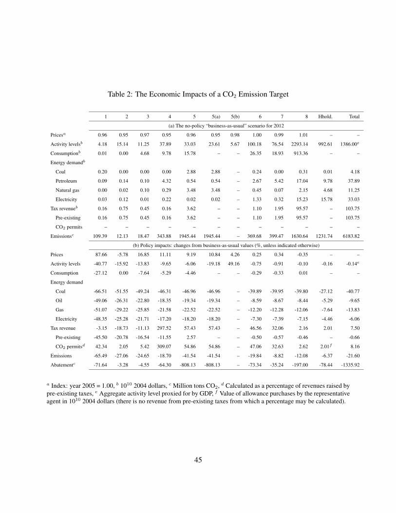
Table 2: The Economic Impacts of a CO2 Emission Target

1 2 3 4 5 5(a) 5(b) 6 7 8 Hhold. Total

(a) The no-policy “business-as-usual” scenario for 2012

Pricesa 0.96 0.95 0.97 0.95 0.96 0.95 0.98 1.00 0.99 1.01 – –

Activity levelsb 4.18 15.14 11.25 37.89 33.03 23.61 5.67 100.18 76.54 2293.14 992.61 1386.00e

Consumptionb 0.01 0.00 4.68 9.78 15.78 – – 26.35 18.93 913.36 – –

Energy demandb

Coal 0.20 0.00 0.00 0.00 2.88 2.88 – 0.24 0.00 0.31 0.01 4.18

Petroleum 0.09 0.14 0.10 4.32 0.54 0.54 – 2.67 5.42 17.04 9.78 37.89

Natural gas 0.00 0.02 0.10 0.29 3.48 3.48 – 0.45 0.07 2.15 4.68 11.25

Electricity 0.03 0.12 0.01 0.22 0.02 0.02 – 1.33 0.32 15.23 15.78 33.03

Tax revenueb 0.16 0.75 0.45 0.16 3.62 – – 1.10 1.95 95.57 – 103.75

Pre-existing 0.16 0.75 0.45 0.16 3.62 – – 1.10 1.95 95.57 – 103.75

CO2 permits – – – – – – – – – – – –

Emissionsc 109.39 12.13 18.47 343.88 1945.44 1945.44 – 369.68 399.47 1630.64 1231.74 6183.82

(b) Policy impacts: changes from business-as-usual values (%, unless indicated otherwise)

Prices 87.66 -5.78 16.85 11.11 9.19 10.84 4.26 0.25 0.34 -0.35 – –

Activity levels -40.77 -15.92 -13.83 -9.65 -6.06 -19.18 49.16 -0.75 -0.91 -0.10 -0.16 -0.14e

Consumption -27.12 0.00 -7.64 -5.29 -4.46 – – -0.29 -0.33 0.01 – –

Energy demand

Coal -66.51 -51.55 -49.24 -46.31 -46.96 -46.96 – -39.89 -39.95 -39.80 -27.12 -40.77

Oil -49.06 -26.31 -22.80 -18.35 -19.34 -19.34 – -8.59 -8.67 -8.44 -5.29 -9.65

Gas -51.07 -29.22 -25.85 -21.58 -22.52 -22.52 – -12.20 -12.28 -12.06 -7.64 -13.83

Electricity -48.35 -25.28 -21.71 -17.20 -18.20 -18.20 – -7.30 -7.39 -7.15 -4.46 -6.06

Tax revenue -3.15 -18.73 -11.13 297.52 57.43 57.43 – 46.56 32.06 2.16 2.01 7.50

Pre-existing -45.50 -20.78 -16.54 -11.55 2.57 – – -0.50 -0.57 -0.46 – -0.66

CO2 permitsd 42.34 2.05 5.42 309.07 54.86 54.86 – 47.06 32.63 2.62 2.01f 8.16

Emissions -65.49 -27.06 -24.65 -18.70 -41.54 -41.54 – -19.84 -8.82 -12.08 -6.37 -21.60

Abatementc -71.64 -3.28 -4.55 -64.30 -808.13 -808.13 – -73.34 -35.24 -197.00 -78.44 -1335.92

a Index: year 2005 = 1.00, b 1010 2004 dollars, c Million tons CO2, d Calculated as a percentage of revenues raised bypre-existing taxes, e Aggregate activity level proxied for by GDP, f Value of allowance purchases by the representativeagent in 1010 2004 dollars (there is no revenue from pre-existing taxes from which a percentage may be calculated).

45

MT, approximately 16% below the 2005 emission level and 22% below the BAU scenario.

The impacts of the policy are shown in Table 2(b). Constraining emissions induces significant

increases in fossil fuel prices, particularly the price of coal, which almost doubles. The price of

electricity rises as well, but only by 9%, reflecting both power generators’ ability to substitute

non-energy intermediate goods and labor and capital for fossil fuels, and the ability of carbon-free

electric generators to expand supply. Thus, on a percentage basis the electricity price increase

is smaller than the rise in the marginal cost of fossil generation, but is twice as large as the rise

in the marginal cost of carbon-free power. Prices of non-energy commodities exhibit a negligi-

ble response, while the price of crude oil and gas mining falls with the demand for that sector’s

output.21

Overall, the output of the energy sectors is sharply curtailed. At one extreme, coal production

declines by 41%, with double-digit declines in the demand for this fuel in every sector. At the other

extreme, the generation of electric power declines by a mere six percent, with reductions in demand

of a similar magnitude in non-energy sectors and three to eight times that in the energy sectors.

However, this aggregate picture belies the fact that the fossil fuel subsector declines by 19%, while

the carbon-free subsector experiences a massive expansion in its output, which increases nearly

50%. As before, the impact on production in non-energy sectors is very slight, with slight declines

in output of less than one percent.

The most vigorous CO2 abatement occurs in coal mining and fossil-fuel electricity generation,

while the largest quantities of emissions are reduced by the fossil power and rest-of-economy sec-

tors, with household consumption, transportation, coal mining and petroleum accounting for most

of the remaining cuts. For the most part, these reductions have a negative impact on the revenue

raised by pre-existing taxes, especially in energy industries. The signal exception is electric power,

whose output is buoyed and prices are moderated by the expansion of carbon-free generation, but

the overall effect of the emission target on revenue from benchmark taxes is less than 1%. This

outcome is in contrast to the recycled revenues from CO2 allowances, which account for an 8%

46

increase in tax revenue over the BAU scenario, and mostly emanate from the electric power, rest-

of-economy and final consumption sectors.

Finally, looking at the impact on the economy as a whole, the shadow price on the emission

target is modest: $17.50 per ton, GDP falls by 0.14% relative to its BAU level, while the decline in

aggregate consumption is slightly larger: 0.16%, all of which suggest that the macroeconomic costs

of the emission target are modest. However, both the price of CO2 and the attendant welfare losses

are much smaller than those computed by Paltsev et al. (2007) using the MIT-EPPA model, a large-

scale multi-regional simulation that resolves emissions of non-CO2 GHGs and their abatement

possibilities in addition to representing the frictions associated with the “putty-clay” character of

capital adjustments (Paltsev et al., 2005). Exploring these and other sources of divergence helps

to shed light on the limitations of the modeling approach pursued thus far, as well as initiate

discussion of methods for addressing them which fall under the rubric of advanced topics that

space constraints prevent me from dealing with here.

8.4 Caveats, and Potential Remedies

Returning to the black-box critique, it is useful to note that underlying the results in Table 2 are

several driving forces whose precise effects on the macroeconomic costs of the policy shock have

not been explicitly quantified. One one hand, decomposition analysis is a structured method for

undertaking this kind of investigation which is gaining popularity because of its ability to accom-

modate simulations with large numbers of sectors, regions and exogenous parameters (see, e.g.,

Harrison et al., 2000; Paltsev, 2001; Böhringer and Rutherford, 2002). On the other hand, con-

structing highly stylized maquette models with a simplified structure and few sectors can also go

a long way toward making the constituent economic interactions transparent. But this also implies

that the present results should be taken with a grain of salt: simplified models such as the CES

economy inevitably gloss over important real-world features of the economy that have potentially

47

important implications for the effects of the policy under consideration. I go on to discuss come of

these caveats below.

The first limitation is that consumption is the only price-responsive category of final uses. The

constant “other final demand” vector implies that the economy’s net export position and level of

investment are both invariant to the emission limit, which is highly unrealistic. Addressing this

shortcoming requires the modeler to disaggregate both gross trade flows and investment and model

them as endogenous variables, with imports and exports specified as functions of the joint effects

of changes in aggregate income and the level of gross-of-carbon-tax domestic prices in relation to

world prices, and investment responding to the forward-looking behavior of households and the

adjustment of saving and investment behavior to the policy shock. The model can then be re-cast

in the format of a small open economy (e.g., Harrison et al., 1997), with imports and exports

linked by a balance-of-payments constraint, and commodity inputs to production and final uses

represented as Armington (1969) composites of imported and domestically-produced varieties.

Specifying and calibrating a fully forward-looking CGE model in the complementarity format

of equilibrium is too complex an undertaking discuss here, and in any case Lau et al. (2002) provide

an excellent introduction to the fundamentals. Recursive dynamic CGE models, which solve for a

sequence of static equilibria chained together by intertemporal equations that update the economy’s

primary factor endowments and adjust the values of key time-varying parameters, have proven far

more popular due to their comparative simplicity. The core of these models’ dynamic process is

an investment equation that uses the values of current-period variables to approximate the theoret-

ically correct intertemporal demand for new capital formation. The realism of the present model

could be markedly improved by enabling aggregate investment to adjust endogenously through the

incorporation of a similar investment demand scheme.

A second limitation is the model’s neglect of the important influences of capital malleability

(the ability to adjust the factor proportions of production processes which employ extant capital)

and intersectoral capital mobility on the short-run costs of emission constraints (Jacoby and Sue

48

Wing, 1999). At issue is the treatment of capital as homogeneous and capable of being friction-

lessly reallocated as relative prices change, which casues to production exhibit complete reversibil-

ity. But in reality, changes in production activity of the magnitude seen in Table 2 would likely

necessitate the scrappage and retrofit of energy-using capital on a massive scale, incurring substan-

tial costs of adjustment. Such frictions may be captured by designating a portion of each sector’s

capital input as extant capital which is responsible for the production of output using a fixed input

proportions technology. The likely consequence will be a substantial reduction in the mobility

of—and returns to—capital, especially in declining sectors, with concomitantly larger abatement

costs and reductions in welfare.

A third limitation is that, like capital, labor is modeled as being in inelastic supply. This,

combined with the full employment assumption typical of many CGE models, implies that the

reduction in the labor demanded by declining fossil fuel and energy-using sectors cannot result

in unemployment. Instead, the wage falls, allowing the labor market to clear and surplus labor

to move to other sectors, where it is re-absorbed. But in reality labor is likely to be far less

mobile, implying that these types of price and quantity adjustments will occur more slowly, with

the appearance of frictional unemployment in the interim. This phenomenon is easily simulated

by introducing a labor supply curve into the model, through which the fall in the wage reduces

the representative agent’s endowment of labor.22 Depending on the value of the labor supply

elasticity the distorted equilibrium may exhibit significant unemployment, but general equilibrium

interactions make it difficult to predict whether the welfare loss from an emission limit will be

larger or smaller than in the inelastic labor supply case.

Lastly, perhaps the biggest deficiency of the current model is the CES assumption itself. Real-

world policy analysis models routinely represent consumers’ and producers’ substitution possibil-

ities using nested CES functions whose substitution elasticities that vary simultaneously among

levels of the nesting structure and across sectors. The present model therefore underestimates the

degree of inter-sectoral heterogeneity in substitution possibilities, implying that the results in Ta-

49

ble 2 are subject to a range of biases in different directions. When faced with these sorts of issues,

analysts typically undertake a sensitivity analysis to compare the results of simulations with dif-

ferent combinations of values for the various parameters in their models. However, the application

of structured uncertainty analysis techniques that employ empirically-derived probability distribu-

tions over input parameters (e.g., Webster and Cho, 2006) has the potential to dramatically enhance

our understanding of the scope and consequences of uncertainties in CGE models’ structure and

assumptions, and thereby generate robust insights into policies’ economic impacts.

9 Summary

This paper has provided a lucid, rigorous and practically-oriented introduction to the fundamentals

of computable general equilibrium modeling. The objective has been to de-mystify CGE models

and their use in analyzing energy and climate policies by developing a simple, transparent and

comprehensive framework within which to conceptualize their structural underpinnings, numeri-

cal parameterization, mechanisms of solution and techniques of application. Beginning with the

circular flow of the economy, the logic and rules of social accounting matrices were developed,

and it was demonstrated how imposing the axioms of producer and consumer maximization on

this conceptual edifice facilitation the construction of a synthetic economy that could then be cal-

ibrated on these data. There followed a description of the techniques of numerical calibration and

solution techniques, and a discussion of their implications for the uniqueness and stability of the

simulated equilibria. The focus then shifted to techniques of application, introducing the kinds of

structural modifications that allow CGE models to analyze the economy-wide impacts of various

price and quantity distortions that arise in energy and environmental policy, which culminated in a

practical demonstration using realistic numerical example.

Despite the broad swath of territory covered by this survey, space constraints have precluded

discussion of many of the methodological tricks of the trade that are standard in CGE analyses of

50

energy and climate policy. In particular, this chapter’s closed-economy focus has paid scant atten-

tion to important issues of trade closure rules, model calibration in the presence of pre-existing im-

port tariffs and/or export levies, or the specification and calibration of multi-region models which

combine SAMs for individual economies with data on interregional trade flows. My hope is that

the base of practical and theoretical knowledge developed here lays the groundwork for the study

of these and other advanced topics in applied general equilibrium analysis.

Notes

1e.g., Panagariya and Duttagupta (2001): “Unearthing the features of CGE models that drive

[their results] is often a time-consuming exercise. This is because their sheer size, facilitated

by recent advances in computer technology, makes it difficult to pinpoint the precise source of a

particular result. They often remain a black box. Indeed, frequently, authors are themselves unable

to explain their results intuitively and, when pressed, resort to uninformative answers...”

2Of the numerous articles that use CGE simulations, the vast majority document only those

attributes of their models that are relevant to the application at hand, or merely write down the

model’s equations with a minimum of explanation. On the other hand, expository books and

manuals are often exhaustively detailed (e.g., Shoven and Whalley, 1992; Ginsburgh and Keyzer,

1997; Lofgren et al., 2002), and those in articles focused on applied numerical optimization (e.g.,

Rutherford 1995; Ferris and Pang 1997) often involve a high level of mathematical abstraction,

neither of which make it easy for the uninitiated to quickly grasp the basics. Finally, although

pedagogic articles (e.g., Devarajan et al 1997; Rutherford 1999; Rutherford and Paltsev 1999;

Paltsev 2004) often provide a lucid introduction to the fundamentals, they tend to emphasize either

models’ structural descriptions or the details of the mathematical software packages used to build

them, and have given short shrift to CGE models’ theoretical basis or procedures for calibration.

3Together, these conditions imply that with unfettered competition firms will continue to enter

51

the economy’s markets for goods until profits are competed away to zero.

4See also the simple example by Paltsev (2004).

5This simply a mathematical statement of Walras’ Law (see e.g., Varian (1992, p. 343).)

6See Kehoe (1998a) for description of an alternative procedure when price data are available.

7Cf. Arndt et al. (2002), who develop a maximum-entropy data assimilation technique for

calibrating substitution elasticities based on auxiliary information on prices and subjective bounds

on parameter values.

8Econometric CGE models have been developed by Jorgenson (1984), McKibbin and Wilcoxen

(1998), McKitrick (1998) and Fisher-Vanden and Ho (2007).

9See, e.g., Wilcoxen (1988) p. 127, especially footnote 2.

10See Dirkse and Ferris (1995); Ferris et al. (2000); Ferris and Kanzow (2002) for details of the

algorithms and discussions of their convergence properties. The seminal theoretical work on this

topic is Garcia and Zangwill (1981).

11Kehoe (1985) indicates that early findings along these lines by Foster and Sonnenschein (1970)

and Hatta (1977) require at least one commodity to be an inferior good, a phenomenon which

practically never arises in applied work on energy policy.

12I am grateful to Tim Kehoe for this insight.

13Kehoe and Whalley (1985) find no evidence of multiplicity in the Fullerton et al. (1981) and

Kehoe and Serra-Puche (1983) tax models, while reports of multiple equilibria are restricted to

models with increasing returns (Mercenier, 1995; Denny et al., 1997).

14Note that, for positive tax rates the tax revenue terms in these expressions are will be non-

negative, satisfying the condition for uniqueness discussed in section 6.2.

15Section 5’s discussion of the invariance of models’ benchmark replication to the values of their

substitution parameters figures prominently here. Imagine two static models, each with different

substitution elasticities, calibrated so as to reproduce the same benchmark SAM in the absence of

policy-induced distortions. An absolute emission limit can be imposed on the first model, and the

52

value of GDP in the resulting distorted equilibrium used to compute an ex-ante equivalent inten-

sity target. Imposing this target on the first model will yield the same distorted equilibrium, but

constraining the second model with this target will have different impacts as a result the alternative

parameterization’s effect on GDP.

16Observe that the revenue raised from all producers is∑E

e=1 ρτRPSεeye, while that received

by renewable producers is∑

e∈ER τRPSεeye. Equating these expressions and canceling τRPS on

both sides of the resulting expression yields the rationing constraint in the text. The implication

is that the marginal financing charge exhibits complementary slackness with respect to the RPS

constraint: the latter is either binding and τRPS > 0, or it is non-binding and τRPS = 0.

17I am grateful to Tom Rutherford for pointing this out to me.

18For details see, e.g., Reinert and Roland-Holst (1992). Gabriel Medeiros of the Bureau of

Economic Analysis provided sterling assistance with the procedure.

19The column disaggregation of the sector was performed very simply: 28.4% of labor, capital

and non-energy intermediate inputs, as well as all of the primary energy resource inputs, were

allocated to carbon-free electricity generation, while the remaining inputs of intermediate goods

and primary factors were allocated to fossil-fuel electricity generation. Sue Wing (2008) develops a

more sophisticated method of disaggregating individual technologies from an aggregate economic

sector.

20Sue Wing and Eckaus (2007) provide an in-depth discussion of the AEEI’s conceptual short-

comings, empirical basis and use in CGE models.

21Note that the price increases shown in the table correspond to the gross-of-CO2 markup prices

of fossil fuels. Net-of-markup fossil fuel prices decline sharply as a consequence of shrinking

demand.

22Balistreri (2002) develops a sophisticated external economies approach in which a slump in

aggregate labor demand induces greater unemployment.

53

References

Armington, P. S. (1969). A theory of demand for products distinguished by place of production.

IMF Staff Papers 16(1), 170–201.

Arndt, C., S. Robinson, and F. Tarp (2002). Parameter estimation for a computable general equi-

librium model: a maximum entropy approach. Economic Modelling 19(3), 375–398.

Balistreri, E. J. (2002). Operationalizing equilibrium unemployment: A general equilibrium exter-

nal economies approach. Journal of Economic Dynamics and Control 26, 347–374.

Baron, R. and Y. Serret (2002). Renewable energy certificates: Trading instruments for the promo-

tion of renewable energy. In Implementing domestic tradeable permits: Recent developments

and future challenges, pp. 105–140. Paris: OECD.

Bergman, L. (2005). CGE modeling of environmental policy and resource management. In K.-G.

Maler and J. R. Vincent (Eds.), Handbook of Environmental Economics Vol. 3, pp. 1273–1306.

Elsevier.

Bhattacharyya, S. C. (1996). Applied general equilibrium models for energy studies: a survey.

Energy Economics 18, 145–164.

Böhringer, C. and T. F. Rutherford (2002). Carbon abatement and international spillovers. Envi-

ronmental and Resource Economics 22(3), 391–417.

Böhringer, C., T. F. Rutherford, and W. Wiegard (2003). Computable general equilibrium analysis:

Opening a black box. Discussion Paper No. 03-56, ZEW, Mannheim, Germany.

Conrad, K. (1999). Computable general equilibrium models for environmental economics and

policy analysis. In J. van den Bergh (Ed.), Handbook of Environmental and Resource Economics,

pp. 1061–1087. Cheltenham: Edward Elgar.

54

Conrad, K. (2001). Computable general equilibrium models in environmental and resource eco-

nomics. In T. Tietenberg and H. Folmer (Eds.), The International Yearbook of Environmental

and Resource Economics 2002/2003, pp. 66–114. Edward Elgar.

Cottle, R. W., J.-S. Pang, and R. E. Stone (1992). The Linear Complementarity Problem. Boston,

MA: Academic Press.

Dakhlia, S. (1999). Testing for a unique equilibrium in applied general equilibrium models. Jour-

nal of Economic Dynamics and Control 23, 1281–1297.

Dawkins, C., T. Srinivasan, and J. Whalley (2001). Calibration. In J. Heckman and E. Leamer

(Eds.), Handbook of Econometrics Vol. 5, pp. 3653–3703. Amsterdam: Elsevier Science.

Denny, K., A. Hannan, and K. O’Rourke (1997). Fiscal increasing returns, unemployment and

multiple equilibria: “evidence” from a computable general equilibrium model. mimeo, Univer-

sity College Dublin, Ireland.

Dirkse, S. P. and M. C. Ferris (1995). The PATH solver: A non-monotone stabilization scheme for

mixed complementarity problems. Optimization Methods and Software 5, 123–156.

Eaves, B. C. and K. Schmedders (1999). General equilibrium models and homotopy methods.

Journal of Economic Dynamics and Control 23, 1249–1279.

Ellerman, A. D. and I. Sue Wing (2003). Absolute vs. intensity-based emission caps. Climate

Policy 3(Supplement 2), S7–S20.

Ferris, M. C. and C. Kanzow (2002). Complementarity and related problems. In P. Pardalos

and M. Resende (Eds.), Handbook of Applied Optimization, pp. 514–530. New York: Oxford

University Press.

55

Ferris, M. C., T. S. Munson, and D. Ralph (2000). A homotopy method for mixed complementarity

problems based on the PATH solver. In D. Griffiths and G. Watson (Eds.), Numerical Analysis

1999, pp. 143–167. London: Chapman and Hall.

Ferris, M. C. and J.-S. Pang (1997). Engineering and economic applications of complementarity

problems. SIAM Review 39(4), 669–713.

Fisher-Vanden, K. and M. S. Ho (2007). How do market reforms affect China’s responsiveness to

environmental policy? Journal of Development Economics 82(1), 200–233.

Foster, E. and H. Sonnenschein (1970). Price distortion and economic welfare. Econometrica 38,

281–297.

Fullerton, D., A. King, J. B. Shoven, and J. Whalley (1981). Corporate tax integration in the United

States: a general equilibrium approach. American Economic Review 71, 677–691.

Garcia, C. and W. I. Zangwill (1981). Pathways to Solutions, Fixed Points, and Equilibria. Engle-

wood Cliffs: Prentice-Hall.

Ginsburgh, V. and M. Keyzer (1997). The Structure of Applied General Equilibrium Models.

Cambridge MA: MIT Press.

Goulder, L. H. (1995). Effects of carbon taxes in an economy with prior tax distortions: An

intertemporal general equilibrium analysis. Journal of Environmental Economics and Manage-

ment 29, 271–297.

Goulder, L. H. (Ed.) (2002). Environmental Policy Making in Economies With Prior Tax Distor-

tions. Northampton MA: Edward Elgar.

Harrison, G. W., T. F. Rutherford, and D. G. Tarr (1997). Quantifying the uruguay round. Economic

Journal 107, 1405–30.

56

Harrison, W. J., J. M. Horridge, and K. Pearson (2000). Decomposing simulation results with

respect to exogenous shocks. Computational Economics 15, 227–249.

Hatta, T. (1977). A theory of piecemeal policy recommendations. Review of Economic Studies 44,

1–21.

Hines, J. R. (1999). Three sides of Harberger triangles. Journal of Economic Perspectives 13,

167–188.

Hosoe, N. (2000). Dependency of simulation results on the choice of numeraire. Applied Eco-

nomics Letters 7, 475–477.

Jacoby, H. D. and I. Sue Wing (1999). Adjustment time, capital malleability, and policy cost.

Energy Journal Special Issue: The Costs of the Kyoto Protocol: A Multi-Model Evaluation,

73–92.

Jorgenson, D. W. (1984). Econometric methods for applied general equilibrium analysis. In

H. Scarf and J. B. Shoven (Eds.), Applied General Equilibrium Analysis, pp. 139–207. Cam-

bridge: Cambridge University Press.

Kehoe, P. J. and T. J. Kehoe (1995). A primer on static applied general equilibrium models. In

P. J. Kehoe and T. J. Kehoe (Eds.), Modeling North American Economic Integration, pp. 1–31.

Boston: Kluwer Academic Publishers.

Kehoe, T. J. (1985). The comparative statics properties of tax models. Canadian Journal of

Economics 18, 314–334.

Kehoe, T. J. (1991). Computation and multiplicity of equilibria. In W. Hildenbrand and H. Son-

nenschein (Eds.), Handbook of Mathematical Economics Vol. IV, pp. 2049–2143. Amsterdam:

North-Holland.

57

Kehoe, T. J. (1998a). Social accounting matrices and applied general equilibrium models. In

I. Begg and S. Henry (Eds.), Applied Economics and Public Policy, pp. 59–87. Cambridge:

Cambridge University Press.

Kehoe, T. J. (1998b). Uniqueness and stability. In A. P. Kirman (Ed.), Elements of General

Equilibrium Analysis, pp. 38–87. Basil Blackwell.

Kehoe, T. J. and J. Serra-Puche (1983). A computational general equilibrium model with en-

dogenous unemployment: An analysis of the 1980 fiscal reform in mexico. Journal of Public

Economics 22, 1–26.

Kehoe, T. J. and J. L. Whalley (1985). Uniqueness of equilibrium in large-scale numerical general

equilibrium models. Journal of Public Economics 28, 247–254.

Lau, M., A. Pahlke, and T. Rutherford (2002). Approximating infinite-horizon models in a com-

plementarity format: A primer in dynamic general equilibrium analysis. Journal of Economic

Dynamics and Control 26, 577–609.

Lofgren, H., R. Harris, and S. Robinson (2002). A standard computable general equilibrium (CGE)

model in GAMS. Microcomputers in Policy Research Working Paper No. 5, International Food

Policy Research Institute, Washington DC.

Lutton, T. and M. LeBlanc (1984). A comparison of multivariate Logit and Translog models for

energy and nonenergy input cost share analysis. Energy Journal 5(4), 45–54.

Mas-Colell, A. (1991). On the uniqueness of equilibrium once again. In W. A. Barnett, B. Cornet,

C. D’Aspremont, J. Gabszewicz, and A. Mas-Colell (Eds.), Equilibrium Theory and Applica-

tions: Proceedings of the Sixth International Symposium in Economic Theory and Econometrics,

pp. 275–296. New York: Cambridge University Press.

58

Mathiesen, L. (1985a). Computation of economic equilibria by a sequence of linear complemen-

tarity problems. Mathematical Programming Study 23, 144–162.

Mathiesen, L. (1985b). Computational experience in solving equilibrium models by a sequence of

linear complementarity problems. Operations Research 33, 1225–1250.

McKibbin, W. and P. J. Wilcoxen (1998). The theoretical and empirical structure of the G-Cubed

model. Economic Modelling 16(1), 123–148.

McKitrick, R. R. (1998). The econometric critique of applied general equilibrium modelling: The

role of functional forms. Economic Modelling 15, 543–573.

Mercenier, J. (1995). Nonuniqueness of solutions in applied general equilibrium models with scale

economies and imperfect competition. Economic Theory 6, 161–177.

Paltsev, S. (2001). The Kyoto Protocol: Regional and sectoral contributions to the carbon leakage.

Energy Journal 22, 53–79.

Paltsev, S. (2004). Moving from static to dynamic general equilibrium economic models (notes

for a beginner in MPSGE). Technical Note No. 4, MIT Joint Program on the Science & Policy

of Global Change.

Paltsev, S., J. Reilly, H. Jacoby, R. Eckaus, J. McFarland, M. Sarofim, M. Asadoorian, and

M. Babiker (2005). The mit emissions prediction and policy analysis (eppa) model: Version

4. Report No. 125, MIT Joint Program for the Science and Policy of Global Change.

Paltsev, S., J. M. Reilly, H. D. Jacoby, A. C. Gurgel, G. E. Metcalf, A. P. Sokolov, and J. F.

Holak (2007). Assessment of U.S. cap-and-trade proposals. Working Paper No. 13176, National

Bureau of Economic Research.

59

Panagariya, A. and R. Duttagupta (2001). The ‘gains’ from preferential trade liberalization in the

CGE models: Where do they come from? In S. Lahiri (Ed.), Regionalism and Globalization:

Theory and Practice, pp. 39–60. London: Routledge.

Perroni, C. and T. F. Rutherford (1998). A comparison of the performance of flexible functional

forms for use in applied general equilibrium modelling. Computational Economics 11(3), 245–

263.

Reinert, K. A. and D. W. Roland-Holst (1992). A detailed social accounting matrix for the USA,

1988. Economic Systems Research 4, 173–87.

Rutherford, T. F. (1987). Implementational issues and computational performance solving applied

general equilibrium models with SLCP. Cowles Foundation Discussion Paper No. 837, Yale

University.

Rutherford, T. F. (1995). Extensions of GAMS for complementarity problems arising in applied

economic analysis. Journal of Economic Dynamics and Control 19, 1299–1324.

Shoven, J. B. and J. L. Whalley (1984). Applied general equilibrium models of taxation and

international trade: An introduction and survey. Journal of Economic Literature 22, 1007–1051.

Shoven, J. B. and J. L. Whalley (1992). Applying General Equilibrium. Cambridge: Cambridge

University Press.

Sue Wing, I. (2001). Induced Technical Change in CGE Models for Climate Policy Analysis. Ph.

D. thesis, Massachusetts Institute of Technology.

Sue Wing, I. (2008). The synthesis of bottom-up and top-down approaches to climate policy mod-

eling: Electric power technology detail in a social accounting framework. Energy Economics In

Press.

60

Sue Wing, I. and R. S. Eckaus (2007). The decline in U.S. energy intensity: Its origins and

implications for long-run CO2 emission projections. Energy Policy 35, 5267U5286.

U.S. EPA (2007). Inventory of U.S. Greenhouse Gas Emissions and Sinks: 1990-2005. Washington

DC: Government Printing Office.

Varian, H. R. (1992). Microeconomic Analysis. New York: Norton.

Webster, M. and C.-H. Cho (2006). Analysis of variability and correlation in long-term economic

growth rates. Energy Economics 28, 653–666.

Whalley, J. and S. Zhang (2002). Tax induced multiple equilibria. mimeo, University of Western

Ontario.

Wilcoxen, P. J. (1988). The Effects of Environmental Regulation and Energy Prices on U.S. Eco-

nomic Performance. Ph. D. thesis, Harvard University.

61