Computable General Equilibrium Models for Pol-icy Evaluation and Economic Consequence Anal-ysis

Ian Sue Wing

Dept. of Earth & Environment, Boston University, 675 Commonwealth Ave., Boston MA

02215

isw@bu.edu

Edward J. Balistreri

Division of Economics and Business, Colorado School of Mines, 816 15th Street, Golden CO

80401

ebalistr@mines.edu

Computable General Equilibrium Models for Pol-icy Evaluation and Economic Consequence Anal-ysis

ABSTRACT

This chapter reviews recent applications of computable general equilibrium (CGE) modeling

in the analysis and evaluation of policies which affect interactions among multiple markets.

At the core of this research is a particular approach to the data and structural representations

of the economy, which we elaborate through the device of a canonical static multiregional

model. We adapt and extend this template to shed light on the structural and methodological

foundations of simulating dynamic economies, incorporating “bottom-up” representations of

discrete production activities, and modeling contemporary theories of international trade

with monopolistic competition and heterogeneous firms. These techniques are motivated

by policy applications including trade liberalization, development, energy policy and green-

house gas mitigation, the impacts of climate change and natural disasters, and economic

integration and liberalization of trade in services.

1 INTRODUCTION

While economic research has historically been dominated by theoretical and econometric

analyses, computational simulations have grown to satisfy the ever-expanding demand for

the assessment of policies in a variety of settings. This third approach complements tra-

ditional economic research methods by marrying a rigorous theoretical structure in an em-

pirically informed context. This chapter offers a review of computable general equilibrium

(CGE) simulations, which have emerged as the workhorse of prospective characterization

and quantification of the impacts of policies which are likely to affect interactions among

multiple markets.

At its core, CGE modeling is a straightforward exercise of “theory with numbers”, where the

latter are dervied from input-output economic accounts and econometric estimates of key

parameters. Advances in computing power and numerical methods have made it possible to

specify and solve models with increasingly complex structural representations of the econ-

omy. These do far more than generate detailed information on the likely impacts of policies

under consideration—their basis in theory enables researchers to pinpoint the economic pro-

cesses that give rise to particular outcomes, and establish their sensitivity to various input

parameters.

Our goal is to rigorously document key contemporary applications of CGE models to the

assessment of the economic impacts of policies ranging from tax reforms to the mitigation

and adaptation of global climate change. Throughout, we focus on the structural repre-

sentation of the economy. In section 2 we begin by deriving the theoretical structure of a

canonical static multi-regional simulation. This model is structurally simple but of arbitrary

dimension, and is sufficiently general to admit the kinds of modifications necessary to ad-

dress a wide variety of research questions and types of policies. We first demonstrate how

our canonical model is general case of ubiquitous single region open-economy models with an

Armington structure, and show how the dynamics of capital accumulation may be introduced

as a boundary condition of the economy (sections 2.2 and 2.3). In section 3 we illustrate

the application of the canonical model in areas which are both popular and well-studied—

international, development and public economics (section 3.1), emerging—energy economics

and greenhouse gas emission abatement (section 3.2) and novel—climate change impacts and

natural hazards (section 3.3). Section 4 moves beyond mere applications to document two

prominent extensions to the canonical framework: the incorporation of discrete technology

detail into representation of production in the sectors of the economy (with a focus on the

electric power sector—section 4.1), and the representation of modern theories of trade based

on heterogeneous firms and the implications for the effects of economic integration (sections

4.2 and 4.3). Section 5 concludes.

2 THE CANONCIAL MODEL

The economic principles underlying a standard closed-economy CGE model are well ex-

plained in pedagogic articles such as Sue Wing (2009, 2011). To conserve space we use these

studies as the point of departure to derive the theoretical structure of a static open-economy

multi-regional CGE model that will be the workhorse of the rest of this chapter, and, in-

deed, has emerged as the standard platform for international economic simulations since its

introduction by Harrison et al. (1997a,b) and Rutherford (2005).

2.1 A Static Multiregional Armington Trade Simulation

The pivotal feature of our model is inter-regional trade in commodities, which follows the

Armington (1969) constant elasticity of substitution (CES) specification. A region’s de-

mands of each commodity are satisfied by an “Armington” composite good, which supplied

by aggregating together domestic and imported varieties of the commodity in question. The

import supply composite is in turn a CES aggregation of quantities of the commodity pro-

duced in other regions, at prices which reflect the markup of transport margins over domestic

production costs. These bilateral commodity movements induce derived demands for inter-

national freight transport services, whose supply is modeled as a CES aggregation of regions’

transportation sector outputs at producer prices.

There are six institutions in the multiregional economy: within each region, households (I1),

investment goods-producing firms (I2), commodity-producing firms (I3), domestic/import

commodity aggregators (I4) and import agents (I5), and, globally, international commodity

transporters (I6). As in Sue Wing (2009, 2011), households are modeled as a representative

agent who derives utility from the consumption of commodities, and is endowed with in-

ternationally immobile factors of production which are rented to domestic goods-producing

firms. In each region, commodity producers in a particular industry sector are modeled as

a representative firm that combines inputs of primary factors and intermediate goods to

generate a single domestic output.

The key departure from the familiar closed-economy model is that domestic output is sold

to commodity aggregators or exported abroad at domestic prices. Regional aggregators of

domestic and imported commodities are modeled as a representative firm that combines

domestic and imported varieties of each commodity into an Armington composite good,

which in turn is purchased by the industries and households in the region in question. The

imported variety of each commodity is supplied by import agents which are modeled as a

representative firm denominated over trade partners’ exports. Finally, each region exports

some of the output of each of its transportation sectors to international shippers, who are

modeled as a global representative firm. Interregional movements of goods generate demands

for international transportation services, with each unit of exports requiring the purchase

of shipping services across various modes. Thus, the economy’s institutions are linked by

Figure 1: Multiregional Accounting Framework

A. Sets B. Arrays

Regions r = 1, . . . ,R Interindustry commodity flows Xr

Commodities i = 1, . . . ,N Primary factor inputs to sectors Vr

Industries j = 1, . . . ,N Final commodity demands Gr

Primary factors f = 1, . . . ,F Of which:

Domestic demands d = consumption (C), Domestic final commodity uses Gd

r

investment (I) Aggregate commodity imports GM

r

Transportation services s ⊂ i International transport service demands GTM

r

Export supplies to other regions GX

r

International transport service supplies GTX

r

C. Benchmark Social Accounting Matrix

← j → ← d → ← r′ 6= r → ← r′ 6= r → Row

1 . . . N C I M 1 . . . R 1 . . . R TX Total

↑ 1 y1,r

i... Xr G

d

r GM

r GTMr G

X

r GTX

r

...

↓ N yN ,r

︸ ︷︷ ︸↑ 1 Gr V 1,r

f... Vr

...

↓ F V F,r

Col.

Total y1 . . . yN GC

r GI

r GM

r GTM

r,1 . . . GTM

r,R GX

r,1 . . . GX

r,R GTX

r

five markets: supply and demands for domestic goods (M1),the Armington domestic-import

composite (M2), imported commodities (M3), international shipping services (M4), and

primary factors (M5).

The values of transactions in these markets are recorded in the cells of interlinked regional

input-output tables in the form of the simplified social accounting matrix (SAM) in Figure

1. This input-output structure is underlain by the price and quantity variables summarized

in Table 1, in which markets correspond to the SAM’s rows and institutions correspond to

Tab

le1:

Sum

mar

yof

Var

iable

sin

the

Can

onic

alM

odel

A.

Inst

itu

tion

s

Ou

tpu

tIn

pu

ts

Pri

ceQ

uanti

tyP

rice

Qu

anti

ty

(I1)

Hou

seh

old

sEr

Un

itex

pen

dit

ure

ur

Uti

lity

leve

lpA i,r

Arm

ingto

ngC i,r

Con

sum

pti

on

dem

an

d

ind

exgood

sp

rice

for

Arm

ingto

ngood

(I2)

Inve

stm

ent

good

spI r

Inve

stm

ent

pri

ceGI r

Aggre

gate

pA i,r

”gI i,r

Inve

stm

ent

dem

an

d

pro

du

cers

inve

stm

ent

for

Arm

ingto

ngood

(I3)

Com

mod

ity

pD j,r

Dom

esti

cy j,r

Dom

esti

cpA i,r

”xi,j,r

Inte

rmed

iate

dem

an

d

pro

du

cers

good

sp

rice

good

ssu

pp

lyfo

rA

rmin

gto

ngood

wf,r

Fact

or

pri

cev f,j,r

Fact

or

dem

an

d

(I4)

Dom

esti

c/im

por

tpA i,r

Arm

ingt

on

qA i,r

Arm

ingto

npD i,r

Dom

esti

cgood

sp

rice

qD i,r

Dom

esti

cgood

ssu

pp

ly

goods

aggr

egat

ors

good

sp

rice

good

ssu

pp

ly

pM i,r

Imp

ort

edgood

sp

rice

qM i,r

Imp

ort

edgood

ssu

pp

ly

(I5)

Imp

ort

agen

tspM i,r

Imp

orte

dqM i,r

Imp

ort

edpD i,r′

Dom

esti

cgood

sgX i,r′ ,r

r’s

imp

ort

sfr

om

good

sp

rice

good

ssu

pp

lypri

ceinr′6=r

oth

erre

gio

nsr′

pT s

Int’

lsh

ipp

ing

gT

Ms,i,r

′ ,r

Int’

ltr

an

sport

serv

ices

serv

ices

pri

ce

(I6)

Inte

rnat

ion

alpT s

Int’

lsh

ipp

ing

qT sIn

t’l

tran

sport

pD s,r

r’s

dom

esti

cg

TX

s,r

Tra

nsp

ort

serv

ice

ship

per

sse

rvic

esp

rice

sup

ply

tran

sport

pri

ceex

port

sfr

omr

B.

Mark

ets

Su

pp

lyD

eman

ds

Pri

ceQ

uanti

ty

(M1)

Dom

esti

cgo

od

spD j,r

y j,r

qD j,r

Dom

esti

cgood

sd

eman

ded

by

Arm

ingto

naggre

gato

r

gX j,r,r

′C

om

mod

ity

exp

ort

s

gT

Xs,r

Inte

rnati

on

al

tran

sport

sale

s(t⊂j)

(M2)

Arm

ingt

ond

omes

tic-

pA i,r

qA i,r

xi,j,r

Inte

rmed

iate

dem

an

dfo

rA

rmin

gto

ngood

imp

ort

com

pos

ite

gC i,r

Con

sum

pti

on

dem

an

dfo

rA

rmin

gto

ngood

gI i,r

Inve

stm

ent

dem

an

dfo

rA

rmin

gto

ngood

(M3)

Imp

orte

dgo

od

spM i,r

gM i,r

qM i,r

Imp

ort

edgood

sd

eman

ded

by

Arm

ingto

naggre

gato

r

(M4)

Inte

rnat

ion

alsh

ipp

ing

serv

ices

pT s

qT sg

TM

s,i,r,r

′M

arg

ins

on

exp

ort

sfr

omr

tooth

erre

gio

nss

(M5)

Pri

mar

yfa

ctor

swf,r

Vf,r

v f,j,r

Good

sp

rod

uce

rs’

dem

an

ds

for

fact

ors

its columns. In line with CGE models’ strength in analyzing the aggregate welfare impacts

of price changes, we reserve special treatment for the households in each region, whose

aggregate consumption we assume generates an economy-wide level of utility (ur) at an

aggregate “welfare price” given by the unit expenditure index (Er). The accounting identities

corresponding to the SAM’s column and row sums are the exhaustion of profit and supply-

demand balance conditions in Figure 2. These make up the core of our CGE model.

Figure 2: The Canonical Model: Accounting Identities and Parameterization

A. Accounting identities based on the SAM

Zero Profit Conditions Supply-Demand Balance Conditions(Institutions) (Markets)

(I1) Erur ≤N∑i=1

pAi,rgCi,r

(I2) pIrGIr ≤

N∑i=1

pAi,rgIi,r

(I3) pDj,ryj,r ≤N∑i=1

pAi,rxi,j,r + wf,rvf,j,r

(I4) pAi,rqAi,r ≤ pDi,rqDi,r + pMi,rq

Mi,r

(I5) pMi,rgMi,r ≤

∑r′ 6=r

(pDi,r′g

Xi,r′,r +

∑r′

pTs gTMs,i,r′,r

)

(I6) pTs qTs ≤

R∑r=1

pDs,rgTXs,r

(M1) yj,r ≥ qDj,r + gTXj,r +

∑r′ 6=r

gXj,r,r′

(M2) qAi,r ≥N∑j=1

xi,j,r + gCi,r + gIi,r

(M3) gMi,r ≥ qMi,rpMi,r

(M4) qTs ≥N∑i=1

R∑r=1

∑r′

gTMs,i,r,r′p

Ts

(M5) Vf,r ≥N∑j=1

vf,j,r

B. Parameters

Institutions Substitution TechnicalElasticities Coefficients

(I1) Households σCr αCi,r Armington good use: consumption

(I2) Investment goods producers σIr αIi,r Armington good use: investment

(I3) Commodity producers σYj,r βi,j,r Intermediate Armington good use

γf,j,r Factor inputs(I4) Domestic/import σDM

i,r ζDi,r Domestic commodity output

commodity aggregators ζMi,r Imported commodities

(I5) Import agents σMMi,r ξi,r′,r Exports to r from other regions s

κt,i,r′,r International transport services(I6) International shippers σTr′ ξt,r Transport service exports from r

To elaborate the model’s algebraic structure we assume that institutional actors possess CES

technology parameterized according to Figure 2.B, and behave in a manner consistent with

consumer and producer optimization. This lets us derive the demand functions that are the

fundamental bridge between the activity levels that reflect institutional behavior and the

prices that establish market equilibrium:

(I1) Representative agents minimize the expenditure necessary to generate each unit of util-

ity subject to the constraint of consumption technology by allocating unit quantities

of each commodity consumed (gCi,r = gCi,r/ur).

mingCi,r

Er =N∑i=1

pAi,rgCi,r

∣∣∣∣∣∣1 =

[N∑i=1

αCi,r(gCi,r)(σC

r −1)/σCr

]σCr /(σ

Cr −1)

.

The result is the unconditional demand for Armington goods inputs to consumption,

gCi,r =(αCi,r)σC

r(pAi,r)−σC

r E σCr ur.

(I2) Investment goods producers minimize the cost of generating a unit of output subject to

the constraint of production technology by allocating unit quantities of commodity

inputs (gIi,r = gIi,r/GIr).

mingIi,r

pIr =N∑i=1

pAi,rgIi,r

∣∣∣∣∣∣1 =

[N∑i=1

αIi,r(gIi,r)(σI

r−1)/σIr

]σIr/(σ

Ir−1)

.

The result is the unconditional demand for Armington goods inputs to investment,

gIi,r =(αIi,r)σI

r(pAi,r)−σI

r(pIr)σI

r GIr.

(I3) Commodity-producing industry sectors minimize the cost of creating a unit of output

subject to the constraint of production technology by allocating purchases of unit

quantities of intermediate commodity inputs and primary factor inputs (xi,j = xi,j/yj

and vf,j = vf,j/yj).

minxi,j,r,vf,j,r

pDj,r =N∑i=1

pAi,rxi,j,r +F∑f=1

wf,rvf,j,r

∣∣∣∣∣∣1 =

[N∑i=1

βi,j,rx(σY

j,r−1)/σYj,r

i,j,r +F∑f=1

γf,j,rv(σY

j,r−1)/σYj,r

f,j,r

]σYj,r/(σ

Yj,r−1)

.

The result is the unconditional demands for intermediate Armington commodity inputs

and nonreproducible primary factor inputs, xi,j,r = βσYj,r

i,j,r

(pAi,r)−σY

j,r(pDj,r)σY

j,r yj,r and

vf,j,r = γσYj,r

f,j,rw−σY

j,r

f,r

(pDj,r)σY

j,r yj,r.

(I4) Domestic/import commodity aggregators minimize the cost of producing a unit of com-

posite output of each commodity subject to the constraint of its CES aggregation

technology by allocating purchases of unit quantities of domestic and imported vari-

eties of the good (qDi,r = qDi,r/qAi,r and gMi,r = qMi,r/q

Ai,r).

minqDi,r,g

Mi,r

pAi,r = pDi,rq

Di,r + pMi,rq

Mi,r

∣∣∣∣1 =

[ζDi,r(qDi,r)(σDM

i,r −1)/σDMi,r + ζMi,r

(qMi,r)(σDM

i,r −1)/σDMi,r

]σDMi,r /(σ

DMi,r −1)

.

The result is the unconditional demand for domestically-produced and imported vari-

eties of each good, qDi,r =(ζDi,r)σDM

i,r(pDi,r)−σDM

i,r(pAi,r)σDM

i,r qAi,r and qMi,r =(ζMi,r)σDM

i,r(pMi,r)−σDM

i,r(pAi,r)σDM

i,r qAi,r.

(I5) Commodity importers minimize the cost of producing a unit of composite import good

subject to the constraint of aggregation technology by allocating purchases of unit

commodity inputs over trade partners’ exports and associated international transport

services (gXi,r′,r = gXi,r′,r/gMi,r and gTM

s,i,r′,r = gTMs,i,r′,r/g

Mi,r). We simplify the problem by

assuming that the export of a unit of commodity i requires fixed quantities of the t

types of transport services (κs,i,r′,r), which enables shipping costs to be specified as

mode-specific markups over the producer prices of overseas goods.

minqMi,r

pMi,r =∑r′ 6=r

(pDi,r′ g

Xi,r′,r +

∑r′

pTs gTMs,i,r′,r

)∣∣∣∣∣∣ gTMs,i,r′,r = κs,i,r′,rg

Xi,r′,r,

1 =

[∑r′ 6=r

ξi,r′,r(gXi,r′,r

)(σMMi,r −1)/σMM

i,r

]σMMi,r /(σMM

i,r −1) .

The result is the unconditional demands for other regions’ exports and for international

transshipment services, gXi,r′,r = ξσMMi,r

i,r′,r

(pDi,r′ +

∑s κs,i,r′,rp

Ts

)−σMMi,r(pMi,r)σMM

i,r gMi,r.

(I6) International shippers minimize the cost of producing a unit of transport service sub-

ject to the constraint of its aggregation technology by allocating purchases of regions’

transportation sector outputs (gTXs,r = gTX

s,r /qTs ).

mingTXs,r

pTs =R∑r=1

pDs,rgTXs,r

∣∣∣∣∣∣1 =

[R∑r=1

χs,r(gTXs,r

)(σTr′−1)/σT

r′

]σTr′/(σ

Tr′−1)

.

The result is the unconditional demand for transport services, gTXs,r = χ

σTss,r

(pDs,r)−σT

s(pTs)σT

s qTs .

Substituting these results into the conditions for (I1)-(I6) and for (M1)-(M6) in Table 2

yields the zero profit conditions (1)-(6) and market clearance conditions (7)-(11) in Figure 2.

These exhibit Karush-Kuhn-Tucker complementary slackness (indicated by “⊥”) with the

activity levels and prices, respectively, in Table 1. There are no markets in the conventional

sense for either consumers’ utility, or, in the present static framework, the investment good.

The latter is treated simply as an exogenous demand (12). Regarding the former, ur is the

highest level of aggregate utility attainable given the values of aggregate household income

(Ir) and the unit expenditure index. This intuition is captured by the market clearance

condition (13), with definition of the income level given by the income balance condition

(14).

Together, (1)-(14) comprise a square system of R(5 + 7N +F) + 2T nonlinear inequalities,

Λ (B), in as many unknowns, B = ur, GIr, yi,r, q

Ai,r, g

Mi,r, q

Ts , p

Di,r, p

Ai,r, p

Mi,r, p

Ts , wf,r, p

Ir,Er,Ir,

Table 2: Equations of the CGE Model

Er ≤

[ N∑i=1

(αCi,r)σC

r(pAi,r)1−σC

r

]1/(σCr −1)

⊥ ur (1)

pIr ≤

[ N∑i=1

(αIi,r)σI

r(pAi,r)1−σI

r

]1/(σIr−1)

⊥ GIr (2)

pDj,r ≤

N∑i=1

βσYj,r

i,j,r

(pAi,r)1−σY

j,r +

F∑f=1

γσYj,r

f,j,rw1−σY

j,r

f,r

1/(1−σYj,r)

⊥ yj,r (3)

pAi,r ≤[(ζDi,r)σDM

i,r(pDi,r)1−σDM

i,r +(ζMi,j,r

)σDMi,r(pMi,r)1−σDM

i,r

]1/(1−σDMi,r )

⊥ qAi,r (4)

pMi,r ≤

∑r′ 6=r

ξσMMi,r

i,r′,r

(pDi,r′ +

R∑r=1

κs,i,r′,rpTs

)1−σMMi,r

1/(1−σMMi,r )

⊥ gMi,r (5)

pTs ≤

[ R∑r=1

χσTsr,t

(pDs,r)1−σT

s

]⊥ qTs (6)

yi,r ≥(ζDi,r)σDM

i,r(pDi,r)−σDM

i,r(pAi,r)σDM

i,r qAi,r

+∑r′ 6=r

ξσMMi,r′

i,r,r′

(pDi,r +

R∑r=1

κs,i,r,r′pTs

)−σMMi,r′ (

pMi,r′)σMM

i,r′ gMi,r′ ⊥ pDi,r (7)

qAi,r ≥(αCi,r)σC

r(pAi,r)−σC

r E σCr ur +

(αIi,r)σI

r(pAi,r)−σI

r(pIr)σI

r GIr

+

N∑j=1

βσYj,r

i,j,r

(pAi,r)−σY

j,r(pDj,r)σY

j,r yj,r ⊥ pAi,r (8)

gMi,r ≥(ζMi,r)σDM

i,r(pMi,r)−σDM

i,r(pAi,r)σDM

i,r qAi,r ⊥ pMi,r (9)

qTs ≥N∑i=1

R∑r=1

∑r′ 6=r

ξσMMi,r

i,r′,r

(pDi,r′ +

∑s

κs,i,r′,rpTs

)−σMMi,r(pMi,r)σMM

i,r gMi,r

⊥ pTs (10)

Vf,r ≥N∑j=1

γσYj,r

f,j,rw−σY

j,r

f,r

(pDj,r)σY

j,r yj,r ⊥ wf,r (11)

GIr given ⊥ pIr (12)

ur ≥ Ir/Er ⊥ Er (13)

Ir =

F∑f=1

wf,rVf,r ⊥ Ir (14)

which constitutes the pseudo-excess-demand correspondence of our multiregional economy.

Numerically calibrating the technical coefficients in Table on a micro-consistent benchmark

multiregional input-output dataset yields our CGE model in a complementarity format:

Λ(B) ≥ 0, B ≥ 0, B′Λ (B) = 0,

which can be solved as a mixed complementarity problem (MCP)—for details, see Sue Wing

(2009). CGE models solve for relative prices, with the marginal utility of income being a

convenient numeraire. A common practice is to designate one region (say r?) as the numeraire

economy by fixing the value of its unit expenditure index, Er? = 1.

2.2 A Single-Region Open-Economy Armington Model

A noteworthy feature of this framework is that it encompasses the single-region open-

economy Armington model as a special case. The latter is specified by omitting international

transport (by dropping eqs. (6) and (10) and the corresponding variables pTs = qTs = 0) and

collapsing bilateral exports and imports into aggregate values GX and GM , which are asso-

ciated with the supply of and demand for an aggregate foreign exchange commodity (with

price PFX). Producers in each industry allocate output between domestic and export mar-

kets according to a constant elasticity of transformation (CET) technology, while imported

quantities of each commodity are a CET function of foreign exchange. The zero profit con-

ditions implied by these assumptions are modifications of eqs. (3) and (5), shown below as

(15) and (16). Applying Shephard’s Lemma to derive the optimal unconditional supplies of

domestic and imported varieties of each good yields the analogues of the market clearance

conditions (7) and (9), shown below as eqs. (17) and (18). The model is closed through the

specification of the current account, with commodity exports generating foreign exchange

according to a CES technology (implying the zero profit condition (19)), and the price of

foreign exchange exhibiting complementary slackness with the current account balance, CAr.

Eq. (20) illustrates the simplest case in which the latter is treated as exogenous, held fixed

at the level prevailing in the benchmark calibration dataset.

[(δDj,r)σY

j,r(pDj,r)1−σY

j,r +(δXj,r)σY

j,r(pXj,r)1−σY

j,r

]1/(1−σYj,r)

≤

[N∑i=1

βσYj,r

i,j,r

(pAi,r)1−σY

j,r +F∑f=1

γσYj,r

f,j,rw1−σY

j,r

f,r

]1/(1−σYj,r)

⊥ yi,r (15)

[N∑i=1

(µMi,r)σM

r(pMi,r)1−σM

r

]1/(1−σMr )

≤ PFXr ⊥ GMr (16)

(δDj,r)σY

j,r(pDj,r)−σY

j,r

×[(δDj,r)σY

j,r(pDj,r)1−σY

j,r +(δXj,r)σY

j,r(pXj,r)1−σY

j,r

]σYj,r/(1−σY

j,r)

yj,r

≥(ζDi,r)σDM

i,r(pDi,r)−σDM

i,r(pAi,r)σDM

i,r qAi,r ⊥ pDi,r (17)

(µMi,r)σM

r(pMi,r)−σM

r

[N∑i=1

(µMi,r)σM

r(pMi,r)1−σM

r

]σMr /(1−σM

r )

GMr

≥(ζMi,r)σDM

i,r(pMi,r)−σDM

i,r(pAi,r)σDM

i,r qAi,r ⊥ pMi,r (18)

PFXr ≤

[N∑i=1

(µXi,r)σX

r(pXi,r)1−σX

r

]1/(1−σXr )

⊥ GXr (19)

GXr −GM

r = CAr ⊥ PFXr (20)

The single-region small open economy model is given by eqs. (1), (2), (15), (4), (16), (17),

(8), (18) and (11)-(20), which comprise a square system of 8+5N +F nonlinear inequalities

in as many unknowns, B = u,GI , yi, qAi , G

Xr , G

Mr , p

Di , p

Ai , p

Mi , wf , p

I ,E ,I ,PFX for a given

region r.

2.3 Introducing Dynamics

An important extension of these basic static frameworks is the introduction of a dynamic

process that enables simulation of economies’ time evolution. The simplest approach is to

construct a “recursive dynamic” model in which factor accumulation is represented by semi-

autonomous increase in the primary factor endowments in xx, and technological progress is

represented by exogenous shifts in the technical coefficients of consumption and production.

Letting t = 1, . . . , T index time, the supply of labor is typically modeled as following an

exogenous trend of population increase (say, ΨPopr,t ) combined with an increasing index of

labor productivity (ΨVL,r,t ≥ 1):

VL,r,t = ΨVL,r,tΨ

Popr,t V L,r (21)

Expansion of the supply of capital is semi-endogenous. Accumulation of regions’ capital

stocks (KSr,t) is driven by investment and depreciation (at rate D) according to the standard

perpetual inventory formulation (22). Investment is determined myopically as a function of

contemporaneous variables in each period’s static MCP, with the simplest assumption being

a constant household marginal propensity to save and invest out of aggregate income (MPSr),

in which case (12) is re-specified as eq. (23). Finally, exogenous rate of return (RKr) are

used to calculate capital endowments from the underlying stocks (22).

KSr,t+1 = GIr,t + (1−D)KSr,t (22)

GIr = MPSr Ir ⊥ pIr (23)

VK,r,t = RKr KSr,t (24)

These equations give rise to a multiregional and multisectoral Solow-Swan model, which,

like its simpler theoretical counterpart, exhibits diminishing returns to accumulating factors

which is compensated for by aggregate productivity growth. Exogenous technical progress

can also be modeled by applying shift parameters that specify a decline in the values of the

coefficients on inputs consumption—αi,r,t = ΨCi,tαi,r, and production—βi,j,r,t = ΨYI

i,j,r,tβi,j,r

and γf,j,r,t = ΨYFf,j,r,tγf,j,r, with ΨC

i,t,ΨYIi,j,r,t,Ψ

YFf,j,r,t ∈ (0, 1]. Production in sector j experiences

neutral technical progress when ΨYIi,j,r,t = ΨYF

f,j,r,t = ΨY

j,r,t. A popular application of biased

technical progress is energy-focused CGE models’ way of capturing the historically-oberved

non-price induced secular decline in the energy-GDP ratio. This is represented via “au-

tonomous energy-efficiency improvement” (AEEI), an exogenously-specified decline in the

coefficient on energy inputs (e ⊂ i) to production and consumption: ΨYIe,j,r,t,Ψ

Ce,t < 1.

The ease of implementation of the recursive-dynamic approach has led to its overwhelming

popularity in applied modeling work, in spite of the limitations of ad-hoc savings-investment

closure rules such as (23) which diverge sharply from the standard economic assumption

of intertemporally optimizing firm and household behavior. The development and applica-

tion of fully forward-looking CGE models has for this reason become an important area of

research. Lau et al. (2002) derive a multisectoral Ramsey model in the complementarity

format of equilibrium, using the consumption Euler equation and the intertemporal budget

constraint of an intertemporal utility maximizing representative agent. The key features of

their framework are a trajectory of aggregate consumption demand determined by exogenous

long-run average rates of interest and discount, the intertemporal elasticity of substitution,

and cumulative net income over the T periods of the simulation horizon, and an intertempo-

ral zero-profit condition for capital stock accumulation dual to (22), which incorporates RKr

as a fully endogenous capital input price index. The resulting general equilibrium problem

is specified and simultaneously solved for all t, which for large-T simulations can dramati-

cally increase the dimension of the pseudo-excess demand correspondence and the associated

complexity and computational cost. It is therefore unsurprising that single-region forward-

looking CGE models1 tend to be far more common than their multiregional counterparts.2

3 THE CANONICAL MODEL AT WORK

3.1 Traditional Applications: International, Development and Pub-

lic Economics

CGE models have long been the analytical mainstay of assessments of trade liberalization

and economic integration (Harrison et al., 1997a,b; Hertel, 1997). Such analysis has been

facilitated by the compilation of integrated trade and input-output datasets such as the

Global Trade Analysis Project (GTAP) database (Narayanan and Walmsley, 2008), which

include a range of data on protection and distortions. Incorporating these data into the

canonical model allows the analyst to construct an initial tariff-ridden status-quo equilibrium

which can be used as benchmark from which to simulate the impacts of a wide variety of

policy reforms.

Multilateral trade negotiations are perhaps the simplest illustrate (e.g., Hertel and Winters,

2006). These typically involve reductions in and inter-regional harmonization of two types of

distortions, which may be conveniently introduced into the canonical model as ad-valorem

taxes or subsidies. The first is export levies or subsidies that drive a wedge between the

domestic and FOB prices of each good, and are represented using the parameter τXi,r ≷ 0. The

second is import tariffs that drive a wedge between CIF prices and landed costs, represented

parametrically by τMi,r > 0. The benefits of this approach are simplicity, as well as the

ability to capture the border effects of various kinds of non-tariff barriers to trade where

empirical estimates of these measures’ “ad valorem equivalents” are available (see, e.g.,

Fugazza and Maur, 2008). Modeling the “shocks” constituted by changes to such policy

parameters follows a standard procedure which we will apply throughout this chapter: first,

modify the zero profit conditions to represent the shcok as a price wedge, second, specify

modifications implied by Hotelling’s lemma to the supply and demand functions in the

market clearance conditions, and third, reconcile the income balance condition with the net

revenues or captured rents. Other extensions to the model structure might be warranted,

depending on the interactions of interest. Adjusting the equations for import zero profit (5),

domestic market clearance (7), and income balance (14) in Table 2, we obtain, respectively,

pMi,r ≤

∑r′ 6=r

ξσMMi,r

i,r′,r

((1 + τMi,r )(1 + τXi,r′)p

Di,r′ +

R∑r=1

κs,i,r′,rpTs

)1−σMMi,r

1/(1−σMMi,r )

⊥ gMi,r (25)

yi,r ≥(ζDi,r)σDM

i,r(pDi,r)−σDM

i,r(pAi,r)σDM

i,r qAi,r +∑r′ 6=r

(1 + τMi,r )(1 + τXi,r′)ξσMMi,r′

i,r,r′

×

((1 + τMi,r′)(1 + τXi,r)p

Di,r +

R∑r=1

κs,i,r,r′pTs

)−σMMi,r′ (

pMi,r′)σMM

i,r′ gMi,r′ ⊥ pDi,r (26)

Ir =F∑f=1

wf,rVf,r +N∑i=1

τXi,rpDi,r

∑r′ 6=r

(1 + τMi,r′)(1 + τXi,r)ξσMMi,r′

i,r,r′

×

((1 + τMi,r′)(1 + τXi,r)p

Di,r +

R∑r=1

κs,i,r,r′pTs

)−σMMi,r′ (

pMi,r′)σMM

i,r′ gMi,r′

+N∑i=1

τMi,r∑r′ 6=r

pDi,r′(1 + τMi,r )(1 + τXi,r′)ξσMMi,r

i,r′,r

×

((1 + τMi,r )(1 + τXi,r′)p

Di,r′ +

R∑r=1

κs,i,r′,rpTs

)−σMMi,r (

pMi,r)σMM

i,r gMi,r ⊥ Ir (27)

The fact that τX and τM are pre-existing distortions means that it is necessary to recali-

brate the model’s technical coefficients to obtain a benchmark equilibrium. Trade policies

are simulated by changing elements of these vectors from their benchmark values and com-

puting new counterfactual equilibria that embody income and substitution effects in both

the domestic economy, r, and its trade partners, r′. The resulting effects on welfare manifest

themselves through the new tax revenue terms in the income balance equation. Hertel et al.

(2007) demonstrate that the magnitude of these impacts strongly depends on the values of

the elasticities governing substitution across regional varieties of each good, σMMi,r .

The breadth and richness of analyses that can be undertaken simply by manipulating dis-

tortion parameters such as tax rates—or the endowments and productivity parameters the

define boundary conditions of the economy, is truly remarkable and should not be underes-

timated.

International economics continues to be a mainstay of the CGE literature, with numerous

articles over the past decade dedicated to assessing the consequences of various trade agree-

ments and liberalization initiatives,3 as well as a variety of multilateral price support schemes

(Psaltopoulos et al., 2011), distortionary trade policies (Naud and Rossouw, 2008; Narayanan

and Khorana, 2014), non-tariff barriers to trade (Fugazza and Maur, 2008; Winchester, 2009),

and internal and external shocks (implemented in the model of section 2.2 by dropping eq.

(18) and fixing the complementary variable pMi,r).4 More analytically-oriented papers have

investigated the manner in which the macroeconomic effects of shocks are modulated by im-

perfect competition (Konan and Assche, 2007), agents expectations (Boussard et al., 2006;

Femenia and Gohin, 2011), and international mechanisms of price transmission (Siddig and

Grethe, 2014). Still others studies advance the state of modeling, extending the canonical

model beyond just trade into the realm of international macroeconomics by introducing for-

eign direct investment and its potential to generate domestic productivity spillovers (Lejour

et al., 2008; Latorre et al., 2009; Deng et al., 2012), and financial assets and interregional

financial flows (Maldonado et al., 2007; Lemelin et al., 2013; Yang et al., 2013). Following

Markusen (2002) and Markusen et al. (2005), the typical approach taken by the latter crop

of papers is to disaggregate capital input as a factor of production into domestic and for-

eign varieties, the second of which is internationally mobile and imperfectly substitutable for

domestic capital.

A related development literature examines a broader range of outcomes in poor countries,

for example the social, environmental and poverty impacts of trade policy and liberaliza-

tion,5 and the economic and social consequences of energy price shocks, energy market

liberalization, and alternative energy promotion 6. Similar studies investigate the macro-

level developng country consequences of productivity improvements generated by foreign aid

(Clausen and Schrenberg-Frosch, 2012), changes in the delivery of public services such as

eduction and health (Debowicz and Golan, 2014; Roos and Giesecke, 2014) or domestic R&D

and industrial policies to simulate economic growth (Breisinger et al., 2009; Bor et al., 2010;

Ojha et al., 2013), and the growth consequences of worker protection and restrictions on

international movements of labor (Ahmed and Peerlings, 2009; Moses and Letnes, 2004).

Yet another perspective on these issues is taken by the public economics literature, which

investigates the economy-wide effects of energy and environmental tax changes (Karami

et al., 2012; Markandya et al., 2013; Zhang et al., 2013), ageing-related and pension policies—

through either a coupled CGE-microsimulation modeling framework (van Sonsbeek, 2010)

or dynamic CGE models embodying overlapping generations of households,7 actual and

proposed tax reforms in developed and developing countries,8 the welfare implications of

decentralized public services provision (Iregui, 2005), and rising wage inequality within the

OECD (Winchester and Greenaway, 2007).

Common to virtually all these studies is the economy-wide impact of a change in one or more

distortions. This is customarily measured by the marginal cost of public funds (MCF): the

effect on money-metric social welfare of raising an additional dollar of government revenue

through changing a particular tax instrument (Dahlby, 2008). GCE models’ strength is their

ability to capture the influence that pre-existing market distortions may have on the MCF

in real-world “second best” policy environments. Distortions interact, potentially offsetting

or amplifying one another, with the result that imposing an additional distortion in an

already tariff-ridden economy may not necessarily worsen welfare, while removing an existing

distortion is not guaranteed to be welfare improving (see, e.g., Ballard and Fullerton, 1992;

Fullerton and Rogers, 1993; Slemrod and Yitzhaki, 2001). CGE models can easily report

the MCF for any given, or proposed instrument, as the ratio of the money-metric welfare

cost to increased tax revenue. Ranking policy instruments based on their MCF gives a good

indication of efficiency enhancing reforms. An instructive example is Auriol and Warlters’

(2012) analysis of the MCF in 38 African countries quantifying the welfare effects of taxes

on domestic production, labor and capital, in addition to imports and exports. Factor taxes

deserve special attention because a tax on a factor that is in perfectly inelastic supply does

not distort allocation, implying that the effects of distortionary factor taxes can only be

represented by introducing price-responsive factor supplies, modifying the market clearance

conditions (11). The most common way to address this is to endogenize the supply of labor

through introducing labor-leisure choice or unemployment (for elaborations see, e.g., Sue

Wing, 2011 and Balistreri, 2002).

3.2 Emerging Applications: Energy Policy and Climate Change

Mitigation

Energy policies, as well as measures to mitigate the problem of climate change through

reductions in economies’ emissions of greenhouse gases (GHGs), are two areas that over

the past decade has been at the forefront of CGE model development and application.

Sticking with the types of parameterically-driven shocks discussed in section 3.1, the energy

economics and policy literature has investigated economic consequences of changing taxes

and subsidies on conventional energy,9 the social and environmental dimensions of energy use

and policy,10 macroeconomic consequences of energy price shocks (He et al., 2010; Aydin and

Acar, 2011; Guivarch et al., 2009), and energy use, efficiency and conservation: and how they

influence, and are affected by, the rate and direction of innovation and economic growth.11

Further technical/methodological studies evaluate the representation of energy technology

and substitution possibilities in CGE models (Schumacher and Sands, 2007; Beckman et al.,

2011; Lecca et al., 2011), and the consequences of, and mitigating effect of policy interventions

on, depletion of domestic fossil fuel reserves in resource-dependent economies (Djiofack and

Omgba, 2011; Barkhordar and Saboohi, 2013; Bretschger and Smulders, 2011).

An important development in energy markets is the widespread expansion of policy initi-

tives promoting alternative and renewable energy supplies. This topic has been an area of

particular growth in CGE assessments.12 In most areas of the world such energy supplies

are more costly to operate than conventional energy production activities. Consequently,

they typically make up a small or non-existent fraction of the extant energy supply, and are

unlikely to be represented in current input-output accounts on which CGE model calibra-

tions are based. To assess the macroeconomic consequences of new energy technologies it is

therefore necessary to introduce into the canonical model new, non-benchmark production

activities whose technical coefficients are derived from engineering cost studies and other

ancillary data sources, whose higher operating costs relative to conventional activities in the

SAM render their operation inactive in the benchmark equilibrium, but which are capable

of endogenously switching on and producing output in response to relative price changes or

policy stimuli.

These so-called “backstop” technology options—indexed by b—are implemented by speci-

fying additional production functions whose outputs are perfect substitutes for an existing

source of energy supply (e.g., electricity, e′). Their associated cost functions embody a pre-

mium over benchmark prices, modeled by the markup factor MKUPe′,r > 1, which can be

offset by an output subsidy τ be′,r < 0:

pDe′,r ≤(1 + τ be′,r

)MKUP b

e′,r ·

[N∑i=1

(βbi,e′,r

)σYe′,r(pAi,r)1−σY

e′,r

+F∑f=1

(γbf,e′,r

)σYe′,r w

1−σYe′,r

f,r +(γbFF,e′,r

)σYe′,r(wbFF,e′,r

)1−σYe′,r

]1/(1−σYe′,r)

⊥ ybe′,r (28)

Note that once τ be′,r ≤ 1/MKUP be′,r − 1 the backstop becomes cost-competitive with conven-

tional supply of e′ and switches on, but an unpleasant side effect of perfect substitutability

is “bang-bang” behavior where a small increase in the subsidy parameter induces a jump

in the backstop’s output, which in the limit can result in the backstop capturing the entire

market (ybe′,r ye′,r). To replace such unrealistic behavior with a smooth path of entry

along which both backstop and conventional supplies coexist, a popular trick is to introduce

into the backstop production function a small quantity of a technology-specific fixed factor

(with price wbFF,e′,r and technical coefficient γbFF,e′,r) whose limited endowment constraints

the output of the backstop, even at favorable relative prices. The impact is apparent from

the fixed-factor market clearance condition:

VFF,e′,r ≥(γbFF,e′,r

)σYe′,r(wbFF,e′,r

)−σYe′,r(pDe′,r

)σYe′,r ybe′,r ⊥ wbFF,e′,r (29)

where, with the fixed-factor endowment (VFF) held constant, the quantity of backstop out-

put increases with the fixed-factor’s relative price,(wbFF/p

D)σY

. Thus, once the elasticity

of substitution between the fixed-factor and other inputs is sufficiently small, even a large

increase in the backsop price results in only modest backstop activity. In dynamic models

the exogenously specified trajectory of VFF is an important device for tuning new technolo-

gies’ penetration to the modeler’s sense of plausibility, especially when the future character

and magnitude of “market barriers”, unanticipated complementary investments or negative

network externalities represented by the fixed-factor constraint are unknown.

A related topic that has seen the emergence of a voluminous literature is climate change

mitigation through policies to limit anthropogenic emissions of greenhouse gases (GHGs).

Carbon dioxide (CO2), the chief GHG, is emitted to the atmosphere primarily from the

combustion of fossil fuels. Policies to curtail fossil fuel use tend to limit the supply of energy,

whose signature characteristics of being an input to virtually every economic activity and

possessing few low-cost substitutes (especially in the short-run) with the upshot that GHG

mitigation policies have substantial general equilibrium impacts (Hogan and Manne, 1977).

The simplest policy instrument to consider is an economy-wide GHG tax. For exposi-

tional clarity we partition the set of commodities and industries into the subset of energy

goods/sectors associated with CO2 emissions (indexed by e, as before) and the complemen-

tary subset of non-energy material goods/sectors, indexed by m. The stoichiometric linkage

between CO2 and the carbon content of the fuel being combusted implies a Leontief rela-

tionship between emissions and the quantity of use of each fossil fuel. This is represented

using fixed emission factors (εCO2e,r ) that transform a uniform tax on emissions (τGHG

r ) into a

vector of differentiated markups on the unit cost of the e Armington energy commodities,

as shown in eq. (30).

This simple scheme cannot be extended to non-CO2 GHGs, the majority of which emanate

from a broad array of industrial processes and household activities but are not linked in

any fixed way to inputs of particular energy or material commodities. Non-CO2 GHGs tar-

geted by the Kyoto Protocol are methane, nitrous oxide, hyrdro- and perfluorocarbons, and

sulfur hexafluaoride, which we index by o = 1 . . .O, and whose global warming impact

in units of CO2-equivalents are given by εGHGo . In an important advance, Hyman et al.

(2003) develop a methodology for modeling non-CO2 GHG abatement by treating these

emissions as (a) inputs to the activities of firms and households, which (b) substitute for

a composite of all other commodity and factor inputs with CES technology. The upshot

is that the impact of a tax on non-CO2 GHGs is mediated through a CES demand func-

tion whose elasticity to the costs of pollution control can be tuned to reproduce marginal

abatement cost curves derived from engineering or partial-equilibrium economic studies. The

key tuning parameters are the technical coefficients on emissions (ϑo,j,r) and the elasticity

of substitution between emissions and other inputs (σGHGo,j,r ). The latter indicates the rela-

tive attractiveness of industrial process changes as a margin of adjustment to GHG price

or quantity restrictions. Eq. (31) highlights the implications for production costs at the

margin, which increase by the product of the unit demand for emissions of each category of

pollutant, (ϑo,j,r)−σGHG

o,j,r(τGHGr εGHG

o

)−σGHGo,j,r

(pDj,r)σGHG

o,j,r , and its effective price (τGHGr εGHG

o ).

pAi,r ≤[(ζDi,r)σDM

i,r(pDi,r)1−σDM

i,r +(ζMi,j,r

)σDMi,r(pMi,r)1−σDM

i,r

]1/(1−σDMi,r )

+

τGHGr εCO2

e,r e ⊂ i

0 otherwise⊥ qAi,r (30)

pDj,r ≤

[N∑i=1

βσYj,r

i,j,r

(pAi,r)1−σY

j,r +F∑f=1

γσYj,r

f,j,rw1−σY

j,r

f,r

]1/(1−σYj,r)

+O∑o=1

(ϑo,j,r)−σGHG

o,j,r(τGHGr εGHG

o

)1−σGHGo,j,r

(pDj,r)σGHG

o,j,r ⊥ pDj,r (31)

Ir =F∑f=1

wf,rVf,r +∑e

τGHGr εCO2

e,r qAe,r

+N∑j=1

O∑o=1

[(ϑo,j,r)

−σGHGo,j,r

(τGHGr εGHG

o

)1−σGHGo,j,r

(pDj,r)σGHG

o,j,r yj,r

]⊥ Ir (32)

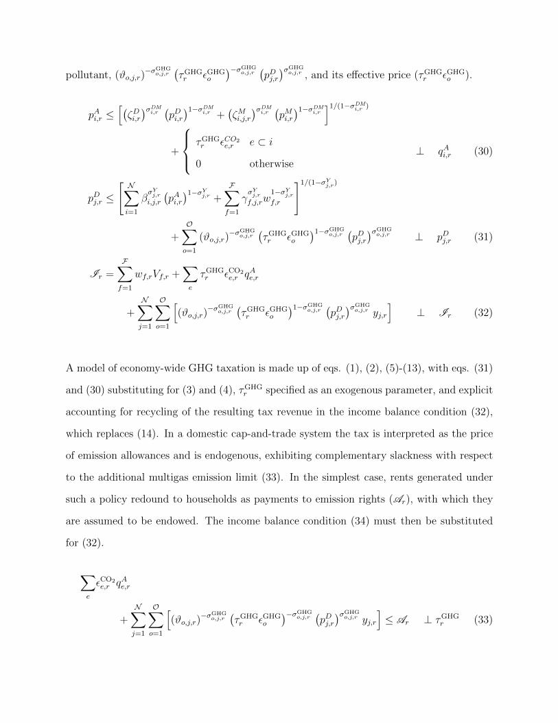
A model of economy-wide GHG taxation is made up of eqs. (1), (2), (5)-(13), with eqs. (31)

and (30) substituting for (3) and (4), τGHGr specified as an exogenous parameter, and explicit

accounting for recycling of the resulting tax revenue in the income balance condition (32),

which replaces (14). In a domestic cap-and-trade system the tax is interpreted as the price

of emission allowances and is endogenous, exhibiting complementary slackness with respect

to the additional multigas emission limit (33). In the simplest case, rents generated under

such a policy redound to households as payments to emission rights (Ar), with which they

are assumed to be endowed. The income balance condition (34) must then be substituted

for (32).

∑e

εCO2e,r qAe,r

+N∑j=1

O∑o=1

[(ϑo,j,r)

−σGHGo,j,r

(τGHGr εGHG

o

)−σGHGo,j,r

(pDj,r)σGHG

o,j,r yj,r

]≤ Ar ⊥ τGHG

r (33)

Ir =F∑f=1

wf,rVf,r + τGHGr Ar ⊥ Ir (34)

A multilateral emission trading scheme over the subset of abating regions, R†, is easily

implemented by dropping the region subscript on the allowance price (τGHGr = τGHG ∀r ∈ R†)

and taking the sum of eq. (33) across regions to specify the aggregate emission limit (35).

The latter, which is the sum of individual regional emission caps (A =∑

r∈R† Ar), induces

allocation of emissions across regions, sectors and gases to equalize the marginal costs of

abatement. The income and/or welfare consequences for an individual region may be positive

or negative depending on whether its residual emissions are below or above its cap, inducing

net purchases or sales of allowances.

∑r∈R†

∑e

εCO2e,r qAe,r

+N∑j=1

O∑o=1

[(ϑo,j,r)

−σGHGo,j,r

(τGHGεGHG

o

)−σGHGo,j,r

(pDj,r)σGHG

o,j,r yj,r

]−A

≤ 0 ⊥ τGHG (35)

Ir =F∑f=1

wf,rVf,r + τGHGAr −∑e

τGHGεCO2e,r qAe,r

−N∑j=1

O∑o=1

[(ϑo,j,r)

−σGHGo,j,r

(τGHGεGHG

o

)1−σGHGo,j,r

(pDj,r)σGHG

o,j,r yj,r

]⊥ Ir (36)

Finally, slow progress in implementing binding regimes for climate mitigation—either an

international system of emission targets or comprehensive economy-wide emission caps at

the national level—has re-focused attention on assessing the consequences of piecemeal policy

initiatives, particularly GHG abatement and allowance trading within sub-national regions

and/or sectors nations. The major consequence is an inability to reallocate abatement across

sources as a way of arbitraging differences in the marginal costs of emission reductions,

which may be captured by differentiating emission limits and their complementary shadow

prices among covered sectors (say j′) and regions (say r′): Aj′,r′ and τGHGj′,r′ . The key concern

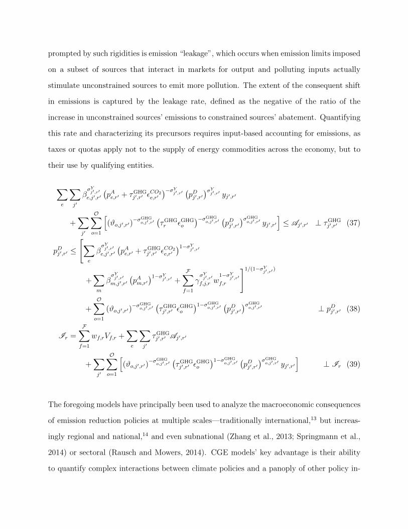
prompted by such rigidities is emission “leakage”, which occurs when emission limits imposed

on a subset of sources that interact in markets for output and polluting inputs actually

stimulate unconstrained sources to emit more pollution. The extent of the consequent shift

in emissions is captured by the leakage rate, defined as the negative of the ratio of the

increase in unconstrained sources’ emissions to constrained sources’ abatement. Quantifying

this rate and characterizing its precursors requires input-based accounting for emissions, as

taxes or quotas apply not to the supply of energy commodities across the economy, but to

their use by qualifying entities.

∑e

∑j′

βσYj′,r′

e,j′,r′

(pAe,r′ + τGHG

j′,r′ εCO2

e,r′

)−σYj′,r′(pDj′,r′

)σYj′,r′ yj′,r′

+∑j′

O∑o=1

[(ϑo,j′,r′)

−σGHGo,j′,r′

(τGHGr εGHG

o

)−σGHGo,j′,r′

(pDj′,r′

)σGHGo,j′,r′ yj′,r′

]≤ Aj′,r′ ⊥ τGHG

j′,r′ (37)

pDj′,r′ ≤

[∑e

βσYj′,r′

e,j′,r′

(pAe,r′ + τGHG

j′,r′ εCO2

e,r′

)1−σYj′,r′

+∑m

βσYj′,r′

m,j′,r′

(pAm,r′

)1−σYj′,r′ +

F∑f=1

γσYj′,r′

f,j,r w1−σY

j′,r′

f,r

]1/(1−σYj′,r′ )

+O∑o=1

(ϑo,j′,r′)−σGHG

o,j′,r′(τGHGj′,r′ ε

GHGo

)1−σGHGo,j′,r′

(pDj′,r′

)σGHGo,j′,r′ ⊥ pDj′,r′ (38)

Ir =F∑f=1

wf,rVf,r +∑e

∑j′

τGHGj′,r′ Aj′,r′

+∑j′

O∑o=1

[(ϑo,j′,r′)

−σGHGo,j′,r′

(τGHGj′,r′ ε

GHGo

)1−σGHGo,j′,r′

(pDj′,r′

)σGHGo,j′,r′ yj′,r′

]⊥ Ir (39)

The foregoing models have principally been used to analyze the macroeconomic consequences

of emission reduction policies at multiple scales—traditionally international,13 but increas-

ingly regional and national,14 and even subnational (Zhang et al., 2013; Springmann et al.,

2014) or sectoral (Rausch and Mowers, 2014). CGE models’ key advantage is their ability

to quantify complex interactions between climate policies and a panoply of other policy in-

struments and characteristics of the economy. While the universe of these elements is too

broad to consider in detail, key issues include the distributional effects of climate policies

on consumers, firms and regions,15 mitigation in second best settings, fiscal policy interac-

tions, and the double dividend,16 alternative compliance strategies such as emission offsets

and the Clean Development Mechanism,17 interactions between mitigation and trade, emis-

sions leakage, and the efficacy of countervailing border tariffs on GHGs embodied in traded

goods,18 the effects of structural change, innovation, technological progress and economic

growth on GHG emissions and the costs of mitigation in various market settings,19 energy

market interactions,20 and the role of discrete technology options on both the supply side

(e.g., renewables and carbon-capture and storage) and the demand side (e.g., conventional

and alternative-fuel transportation).21

3.3 New Horizons: Assessing the Impacts of Climate Change and

Natural Hazards

Turning now to the flip-side of mitigation, the breadth and variety of pathways through which

the climate influences economic activity are enormous (Dell et al., 2014), and improved un-

derstanding of these channels has spurred the growth of a large literature on the impacts

of climate change. CGE models have the unique capability to represent in a comprehensive

fashion the regional and sectoral scope of climatic consequences—if not their detail—and can

easily accommodate region- and sector-specific damage functions from the impacts of climate

change. However, this advantage comes at the cost of inability to capture intertemporal feed-

backs. Following from the discussion in Section 2.3, despite recent progress in intertemporal

CGE modeling, computational constraints often limit the resolution of these machines to a

handful of regions and sectors and a short time-horizon. Thus, as summarized in Table 3, a

common feature of the CGE models in this are of application is that they are either static

Table 3: CGE Studies of Climate Change: Impacts and Adaptation

Studies Regions Sectoral Focus Models Employed

Deke et al. (2001) Global Agriculture, DART (Klepper et al., 2003)

(11 regions) Sea-level rise

Darwin (1999) Global Agriculture FARM (Darwin et al., 1995)

Darwin et al. (2001) (8 regions) Sea level rise

Jorgenson et al. (2004) U.S. Agriculture, Forestry IGEM

(1 region) Water, Energy, (Jorgenson and Wilcoxen, 1993)

Air quality, Heat stress,

Coastal protection

Bosello et al. (2006) Global Health GTAP-EF (Roson, 2003)

Bosello and Zhang (2006) (8 regions) Agriculture

Bosello et al. (2007) Energy demand

Bosello et al. (2007) Sea level rise

Berrittella et al. (2006), Global Tourism, Couples HTM (Hamilton et al.,

Bigano et al. (2008) (8 regions) Sea level rise 2005) with GTAP-EF

Eboli et al. (2010) Global Agriculture, Tourism, ICES

Bosello et al. (2010a) (14 regions) Health, Energy demand, Couples AD-WITCH

Sea level rise (Bosello et al., 2010b) with ICES

Ciscar et al. (2011) Europe Agriculture, Sea-level rise, GEM-E3 (Capros et al., 1997)

(5 regions) Flooding, Tourism

simulations of a future time period (e.g., Roson, 2003; Bosello and Zhang, 2006; Bosello

et al., 2007) or recursive dynamic simulations driven by contemporaneously-determined in-

vestment (e.g., Deke et al., 2001; Eboli et al., 2010; Ciscar et al., 2011), with 2050 being the

typical simulation horizon. Consequently, they tend to simulate the welfare effects of pas-

sive market adjustments to climate shocks, or, at best, “reactive” contemporaneous averting

expenditures in sectors and regions, but not proactive investments in adaptation.

Table 3 indicates that, apart from a few studies (Jorgenson et al., 2004; Eboli et al., 2010;

Ciscar et al., 2011; Bosello et al., 2012), CGE analyses tend to investigate the broad multi-

market effects of one or two impact endpoints at a time. The latter are derived by forcing

global climate models with various scenarios of GHG emissions to calculate changes in climate

variables at the regional scale, generating response surfaces of temperature, precipitation or

sea-level rise that are then run through natural science or engineering-based impact models

to generate a vector of impact endpoints of particular kinds. These “impact factors” are a

region × sector array of exogenous shocks which are inputs to the model’s counterfactual

simulations.

Shocks fall into three basic categories. First, they affect the supply of climatically exposed

primary factors such as land (Deke et al., 2001; Darwin et al., 2001), which we denote

IF Fact.f,r ∈ (0, 1), and scale the factor endowments in the model. The factor market clearance

and income balance conditions (11) and (14) are then:

IF Fact.f,r Vf,r ≥

N∑j=1

γσYj,r

f,j,rw−σY

j,r

f,r

(pDj,r)σY

j,r yj,r ⊥ wf,r (40)

Ir =F∑f=1

wf,rIF Fact.f,r Vf,r ⊥ Ir (41)

Second, impact factors affect sectors’ transformation efficiency (see, e.g., Jorgenson et al.,

2004), thereby acting as productivity shift parameters in the unit cost function, where adverse

impacts drive up both the marginal cost of production and reduce affected sectors’ demands

for inputs according to the scaling factor IF Prod.f,r ∈ (0, 1). As a consequence, the zero profit

and market clearance conditions (3) and (8) become:

pDj,r ≤(IF Prod.

j,r

)−1

[N∑i=1

βσYj,r

i,j,r

(pAi,r)1−σY

j,r +F∑f=1

γσYj,r

f,j,rw1−σY

j,r

f,r

]1/(1−σYj,r)

⊥ yi,r (42)

qAi,r ≥(αCi,r)σC

r(pAi,r)−σC

r E σCr ur +

(αIi,r)σI

r(pAi,r)−σI

r(pIr)σI

r GIr

+N∑j=1

(IF Prod.

j,r

)σYj,r−1

βσYj,r

i,j,r

(pAi,r)−σY

j,r(pDj,r)σY

j,r yj,r ⊥ pAi,r (43)

Third, impact factors affect the efficiency of inputs to firms’ production and households’

consumption activities. Perhaps the clearest example of this is the impact of increased

temperatures on the demands for heating and cooling services, and in turn electric power.

Such warranted increases in the consumption of climate-related inputs can be treated as a

biased technological retrogression which increases the coefficient on the relevant commodities

(say, i′) in the model’s cost and expenditure functions: IF Inputi′,j,r > 1 and IF Input

¬i′,j,r = 1. Here,

zero profit in consumption (1) and eqs. (3) and (8) become:

Er ≤

[N∑i=1

(αCi,r)σC

r

(pAi,r/IF Input

i,Hhold.,r

)1−σCr

]1/(σCr −1)

⊥ ur (44)

pDj,r ≤

[N∑i=1

βσYj,r

i,j,r

(pAi,r/IF Input

j,r

)1−σYj,r

+F∑f=1

γσYj,r

f,j,rw1−σY

j,r

f,r

]1/(1−σYj,r)

⊥ yi,r (45)

qAi,r ≥(αCi,r)σC

r

(pAi,r/IF Input

i,Hhold.,r

)−σCr

E σCr ur +

(αIi,r)σI

r(pAi,r)−σI

r(pIr)σI

r GIr

+N∑j=1

βσYj,r

i,j,r

(pAi,r/IF Input

i,Hhold.,r

)−σYj,r (

pDj,r)σY

j,r yj,r ⊥ pAi,r (46)

In each instance, intersectoral and interregional adjustments in response to impacts, and the

consequences for sectoral output, interregional trade and regional welfare, can be computed.

The magnitude of damage to the economy due to climate change estimated by CGE studies

varies according to the scenario of warming or other climate forcing used to drive impact

endpoints, the sectoral and regional resolution of both the resulting shocks and the models

used to simulate their economic effects, and the latter’s substitution possibilities. Table 4

gives a sense of the relevant variation across six studies that focus on the economic con-

sequences of different endpoints circa 2050. The magnitude of economic consequences is

generally small, rarely exceeding one tenth of one percent of GDP. Effects also vary in sign,

with some regions benefiting from increased output while others sustaining losses. While

there does not appear to be obvious systematic variation in the sign of effects, either across

different endpoints or among regions, uncovering relevant patterns is complicated by a host

of confounding factors. The studies use different climate change scenarios, and for each

impact category economic shocks are constructed from distinct sets of empirical and mod-

eling studies, each with its own regional and sectoral coverage, using different procedures.

The influence that such critical details have on model results difficult to discern because the

unavoidable omission of modeling details necessitated by journal articles terse exposition.

In particular, the precise steps, judgment and assumptions involved in constructing region-

by-sector arrays of economic shocks out of inevitably patchy empirical evidence tends to be

reported only in a summary fashion. Strengthening the empirical basis for such input data,

and documenting in more detail the analytical procedures to generate IF Fact.f,j,r , IF Prod.

j,r and

IF Inputi′,j,r , will go a long way toward improving the replicability of studies in this literature.

Indeed, this area of research is rich with opportunities for interdisciplinary collaboration

among modelers, empirical economists, natural scientists and engineers.

Recent large-scale studies define the state of the art in this regard. In the PESETA study

of climate impacts on Europe in the year 2050 (Ciscar et al., 2009, 2011, 2012), estimates

of physical impacts were constructed by propagating a consistent set of climate warming

scenarios through different process simulations in four impact categories: agriculture (Iglesias

et al., 2012), flooding (Feyen et al., 2012), sea-level rise (Bosello et al., 2012), and tourism

(Amelung and Moreno, 2012). These “bottom-up” results were then incorporated into the

GEM-E3 model using a variety of techniques to map the endpoints to the types of effects on

economic sectors (Ciscar et al., 2012). Estimated changes in crop yields were implemented as

neutral productivity retrogressions in the agriculture sector. Flood damages were translated

into additional unproductive expenditures by households, secular reductions in the output

of the agriculture sector, and reductions in the outputs of and capital inputs to industrial

and commercial sectors. Changes in visitor occupancy were combined with “per bed-night”

expenditure data to estimate changes in tourist spending by country, and in turn expressed as

secular changes in exports of GEM-E3’s market services sector. Costs of migration induced by

land lost to sea-level rise are incurred by households as additional expenditures, while related

coastal flooding is assumed to equiproportionally reduce sectors endowments of capital. (The

direct macroeconomic effects of reduced land endowments were not considered.)

In Bosello et al. (2012), estimates of the global distribution of physical impacts in six cate-

Table 4: Costs of Climate Change impacts to year 2050: Selected CGE Modeling Studies

Forcing Scenarioand Input Data

Impact Endpoints, Economic Shocksand Damage Costs

Agriculture (Bosello and Zhang, 2006)

0.93C global meantemperature rise;temperature-agricultural outputrelationshipcalculated by FUND

Endpoints considered: temperature, CO2 fertilization effects on agricultural pro-ductivity

Shocks: land productivity in crop sectors

Change in GDP from baseline: 0.006-0.07% increases in rest of Annex 1 regions,0.01-0.025% loss in USA and energy exporting countries, -0.13% loss in the restof the world

Energy Demand (Bosello et al., 2007)

0.93C global meantemperature rise;temperature-energydemand elasticitiesfrom De Cian et al.(2013)

Endpoints considered: temperature effects on demand for 4 energy commodities

Shocks: productivity of intermediate and final energy uses

Change in GDP from baseline: 0.04-0.29% loss in remaining Annex I (developed)regions, 0.004-0.03% increase in Japan, China/India and the rest of the world,0.3% loss in energy exporting countries. Results for perfect competition only.

Health (Bosello et al., 2006)

1C global meantemperature rise;temperature-diseaseand disease-costrelationshipsextrapolated fromnumerous empiricaland modeling studies

Endpoints considered: malaria, schistosomiasis, dengue fever, cardiovascular dis-ease, respiratory ailments, diarrheal disease

Shocks: labour productivity, increased household expenditures on public and pri-vate health care, reduced expenditures on other commodities

Direct costs/benefits (% of GDP): 9% in US and Europe, 11% in Japan and theremainder of the Annex 1, 14% in Eastern Europe and Russia, benefits of 1% inenergy exporters and 3% in the rest of the world

Change in GDP from baseline: 0.04-0.08% increase in Annex 1 regions, 0.07-0.1% loss in energy exporting countries and the rest of the world

Sea level rise/Tourism (Bigano et al., 2008)

Uniform global 25cmsea level rise; landloss calculated byFUND

Endpoints considered: land loss, change in tourism arrivals as a function of landloss

Shocks: reduction in land endowment

Direct costs (% of GDP): < 0.005% loss in most regions, 0.05% in North Africa,0.1-0.16% South- and South-East Asia and 0.24% in Sub-Saharan Africa. Costsare due to land loss only.

Change in GDP from baseline: < 0.0075% loss in most regions, 0.06% in SouthAsia and 0.1% in South-East Asia

Ecosystem services (Bosello et al., 2011)

1.2C/3.1Ctemperature rise,with and withoutimpacts onecosystems

Endpoints considered: timber and agricultural production, forest/cropland/grassland carbon sequestration

Shocks: reduced land productivity, reduced carbon sequestration resulting in in-creased temperature change impacts on 5 endpoints in Eboli et al. (2010)

Change in GDP (3.1C, 2001-2050 NPV @ 3%): $22-$32Bn additional loss in E.and Mediterranean Europe, $5Bn reduction in loss in N. Europe

Water Resources (Calzadilla et al., 2010)

Scenarios of rainfedand irrigated cropproduction,irrigation efficiencybased on Rosegrantet al. (2008)

Endpoints considered: crop production

Shocks: supply/productivity of irrigation services

Change in Welfare: losses in 5 regions range from $60M in Sub-Saharan Africato $442M in Australia/New Zealand, gains in 11 regions range from $180M in therest of the world to $3Bn in Japan/Korea

gories in the year 2050 were derived from the results of different process simulations forced

by a 1.9C global mean temperature increase. Endpoints were expressed as shocks within

the ICES model. Regional impacts on energy and tourism were treated as shocks to house-

hold demand. Changes in final demand for oil, gas, and electricity (based on results from a

bottom-up energy system simulation— Mima et al., 2011) were expressed as biased produc-

tivity shifts in the aggregate unit expenditure function. A two-track strategy was adopted

to simulate changes in tourism flows (arrival changes from an econometrically-calibrated

simulation of tourist flows— Bigano et al., 2007), with non-price climate-driven substitution

effects captured through secular productivity biases which scale regional households demands

for market services (the ICES commodity which includes recreation), and the corresponding

income effects imposed as direct changes in regional expenditure. Regional impacts on agri-

culture and forestry, health, and the effects of river floods and sea-level rise, were treated

as supply-side shocks. Changes in agricultural yields (generated by a crop simulation—

Iglesias et al., 2011) and forest net primary productivity (simulated by a global vegetation

model— Bondeau et al., 2007; Tietjen et al., 2009) were represented as exogenous changes

in the productivity of the land endowment in the agriculture sector and the natural resource

endowment in the timber sector, respectively. The impact of higher temperatures on em-

ployment performance was modeled by reducing aggregate labour productivity (based on

heat and humidity effects estimated by Kjellstrom et al., 2009). Losses of land and buildings

due to sea-level rise (whose costs were derived from a hydrological simulation— Van Der

Knijff et al., 2010) were expressed as secular reductions in regional endowments of land and

capital, which are assumed to decline by the same fraction. Damages from river flooding

span multiple sectors and are therefore imposed using different methods: reduction of the

endowment of arable land in agriculture and equiproportional reduction in the productiv-

ity of capital inputs to other industry sectors, as well as reductions in labour productivity

(equivalent to a one-week average annual loss of working days per year in each region) for

affected populations.

An important aspect of climate impacts assessment that is ripe for investigation is the ap-

plication of CGE models to evaluate the effects of specific adaptation investments. Work in

this area is currently limited by a lack of information about the relevant technology options,

and pervasive uncertainty about the magnitude, timing, and regional and sectoral incidence

of various types of impacts. The difficult but essential work of characterizing adaptation

technologies that are the analogues of those in section 3.2 will render similar analyses for re-

active adaptation straightforward. Moreover, Bosello et al.’s (2010a) methodological advance

of coupling a CGE model with an optimal growth simulation of intertemporal feedbacks on

the accumulation of stock adaptation capacity (Bosello et al., 2010b) paves the way to model

proactive investment in adaptation.

Similar issues arise in CGE analyses of the macroeconomic costs of natural and man-made

hazards (Rose, 2005; Rose et al., 2004; Rose and Guha, 2004; Rose and Liao, 2005; Rose

et al., 2009; Dixon et al., 2010). The key distinction that must be made is between the three

types of impact factors. The parameter IF Fact.i,j,r captures components of damage that cause

direct destruction of the capital stock (e.g., earthquakes, floods or terrorist bombings) or

reduction in the labor supply (e.g., morbidity/mortality or evacuation of populations from

the disaster zone). Second, IF Prod.j,r captures impacts that reduce sectors’ productivity while

leaving factor endowments intact, such as utility lifeline outages (Rose and Liao, 2005) or

pandemic disease outbreaks where workers in many sectors shelter at home as a precaution

(Dixon et al., 2010). Third, IF Inputi′,j,r can be used to model input-using biases of technical

change in the post-disaster recovery phase, e.g., increased demand for construction services.

The fact that these input parameters must often be derived from engineering loss estimation

simulations such as the US Federal Emergency Management Agency’s HAZUS software raises

additional methodological issues. Principal among these are the need to specify reductions in

the aggregate endowment of capital input that are consistent with capital stock losses across

a range of sectors, and to reconcile them with exogenous estimates of industry output losses

for the purpose of isolating non-capital related shocks to productivity. The broader concern,

which applies equally to climate impacts, is the extent to which the methods used to derive

the input shocks inadvertently incorporate the kinds of economic adjustments that CGE

model is tasked with simulating—leading to potential double-counting of both losses and

the mitigating effects of substitution. These questions are the subject of ongoing research.

4 EXTENSIONS TO THE STANDARD MODEL

4.1 Production Technology: Substitution Possibilities, Bottom-

Up vs. Top-Down

In the vast majority of CGE models firms’ technology is specified using hierarchical or nested

CES production functions, whose properties of monotonicity and global regularity facilitate

the computation of equilibrium (Perroni and Rutherford, 1993, 1998), while providing the

flexibility to capture complex patterns of substitution among capital, labor, and interme-

diate inputs of energy and materials. A key consequence of this modeling choice is that

numerical calibration of the resulting model to a SAM becomes a severely under-determined

problem, with the number of model parameters greatly exceeding the degrees of freedom in

the underlying benchmark calibration dataset.

It is common for both the nested structure of production and the corresponding elasticity

of substitution parameters to be be selected on the basis of judgment and assumptions, a

practice which has long been criticized by mainstream empirical economists (e.g., Jorgenson,

1984). While econometric calibration of CGE models’ technology has traditionally been

restricted to flexible functional forms such as the Translog (McKitrick, 1998; McKibbin and

Wilcoxen, 1998; Fisher-Vanden and Sue Wing, 2008; Fisher-Vanden and Ho, 2010; Jin and

Jorgenson, 2010), there has been recent interest in estimating nested CES functions (van der

Werf, 2008; Okagawa and Ban, 2008). Progress in this area continues to be hampered by

lack of data, owing to the particular difficulty of compiling time-sequences of input-output

datasets with consistent price and quantity series. In an attempt to circumvent this problem,

various approaches have been developed for calibrating elasticity parameters to reproduce

empirically estimated input price elasticities (e.g., Arndt et al., 2002; Adkins et al., 2003;

Gohin, 2005), but these have yet to be widely adopted by the CGE modeling community.

A parallel development is the trend toward modifying CGE models’ specification of pro-

duction to incorporate discrete “bottom-up” technology options. This has been especially

popular in climate change mitigation research, where it enables CGE models to capture the

effects of GHG abatement measures on the competition between conventional and alternative

energy technologies, and to simulate the general equilibrium incidence of policies to promote

“green” energy supply or conversion options such as renewable electricity or hybrid electric

vehicles. The incorporation of bottom-up detail in CGE models marries the detail of primal

partial equilibrium activity analysis simulations with general equilibrium feedbacks of price

and substitution adjustments across the full range of consuming sectors in the economy. This

hybrid modeling approach has been used in energy technology assessments relating to trans-

portation (Schafer and Jacoby, 2005) and fuel supply (Chen et al., 2011), its most popular

are of application is prospective analyses of electric power production, an example of which

we provide below.

Methods for incorporating discrete technology detail and substitution in CGE models break

down into two principal classes, namely the “decomposition” approach of Bohringer and

Rutherford (2008, 2009) and Lanz and Rausch (2011) and the “integrated” approach of

Bohringer (1998). The first method simulates a top-down CGE model in tandem with a

bottom-up energy technology model iterating back and forth to convergence.22 Briefly, the

representative agent in the top-down model is “endowed” with quantities of energy supplied

Figure 3: A Bottom-Up/Top-Down Model of Electric Power Production

Sectoral output(yEle,r)

Transmission &distribution

(qTDr )

vTDL,rvTD

K,r← xTDm,r →

σTDr

Totalelectricity supply

(qLoadr )

Base supply(qBaser )

← qTechλ(Base,z),r →

σBaser

Intermediate supply(qIntr )

← qTechλ(Int,z),r →

σIntr

Peak supply(qPeakr )

← qTechλ(Peak,z),r →

σPeakr

σLoadr

σYEle,r

Fossil fuelgeneration

technologies(qTechz,r )

← xTechm,z,r →xTech

φ(e,z),rvTechL,z,rvTech

K,z,r

σTech

Resourcegeneration

technologies(qTechz,r )

← xTechm,z,r →vTech

φ(ff,z),rvTechL,z,rvTech

K,z,r

σTech

by the various active technology options, which it uses to compute both the prices of the

inputs to and outputs of the energy supply sectors, and the levels of aggregate demand for

energy commodities. These results are passed as inputs to the bottom-up model to compute

the aggregate cost-minimizing mix of energy supply, conversion or demand activities, whose

outputs are used to update the top-down model’s endowments at the subsequent iteration.

The second approach embeds activity-analysis representations of bottom-up technology op-

tions directly into a top-down model’s sectoral cost functions, numerically calibrating discrete

activities’ inputs and outputs to be jointly consistent with ancillary statistics and the social

accounts. The key requirement is a consistent macro-level representation of sub-sectoral tech-

nology options and their competition in both input and output markets, which is precisely

where the nested CES model of production proves useful.

To illustrate what the integrated approach involves, we consider a simplified version of the

top-down/bottom-up model of electricity production in Sue Wing (2006, 2008). Figure 3

shows the production structure, which divides the sector into five activities. Delivered elec-

tricity (A1) is a CES function of transmission and distribution (A2) and aggregate electricity

supply (A3). Transmission and distribution is a CES function of labor, capital, intermedi-

ate non-fuel inputs, while aggregate electricity supply is a CES aggregation of three load

segments ` = peak, intermediate, base. Each load segment (A4) is a CES aggregation of

subsets of the z generation outputs, defined by the mapping from load to technology λ(`, z).

Lastly, individual technologies (A5) produce electricity from labor, capital, non-energy ma-

terials and either fossil fuels (e ⊂ i) or “fixed-factor” energy resources (ff ⊂ f) in the case of

nuclear, hydro or renewable power. The latter are defined by the fuel-to-technology mappings

φ(e, z) and φ(ff, z).

Several aspects of this formulation merit discussion. First, substitutability between trans-

mission and the total quantity of electricity generated by the sector captures the fact that

transmission investments’ reductions in congestion and line losses can maintain the level of

delivered power with less physical energy, at least over a small range, suggesting the substi-

tution elasticity value σYEle,r 1. Second, while disaggregation of electricity supply—rather

than demand—into load segments may seem counterintuitive, it is a conscious choice driven

by the exigencies of data availability and model tractability. Demand-side specification of

load segments necessitates row disaggregation of the SAM into separate accounts for indi-

vidual users’ demands for peak, intermediate and base power. The necessary information is

simply not available, which motivates the present structure that is designed to keep deliv-

ered electric power as a homogeneous commodity while differentiating generation by different

technologies. This device is meant to capture the fact that only subsets of the universe of

Tab

le5:

Sum

mar

yof

Var

iable

sin

the

Bot

tom

-Up/T

op-D

own

Model

ofE

lect

ric

Pow

erP

roduct

ion

A.

Act

ivit

ies

Ou

tpu

tIn

pu

ts

Pri

ceQ

uanti

tyP

rice

Qu

anti

ty

(A1)

Sec

tora

lpD Ele,r

Dom

esti

cd

eliv

ered

y Ele,r

Dom

esti

cd

eliv

ered

pTD

rT

ran

smis

sion

qTD

rT

ran

smis

sion

outp

ut

elec

tric

ity

pri

ceel

ectr

icit

ysu

pp

ly&

dis

trib

uti

on

&dis

trib

uti

on

pLoad

rA

ggre

gate

qLoad

rA

ggre

gate

gen

erati

on

pri

cegen

erati

on

(A2)

Tra

nsm

issi

onpTD

rT

ran

smis

sion

qTD

rT

ran

smis

sion

pA m,r

Arm

ingto

nm

ate

rialxTD

m,r

Arm

ingto

nm

ate

rial

&d

istr

ibu

tion

pri

cesu

pp

lygood

spri

cegood

sd

eman

d

wL,r

Wage

vTD

L,r

Lab

or

dem

an

d

wK,r

Cap

ital

renta

lra

tevTD

K,r

Cap

ital

dem

an

d

(A3)

Tot

alel

ectr

icit

ypLoad

rE

lect

rici

tyqL

oad

rE

lect

rici

typLoad

`,r

Ele

ctri

city

pri

ceq` r

Ele

ctri

city

sup

ply

sup

ply

pri

cesu

pp

lyby

load

segm

ent

by

load

segm

ent

(A4)

Loa

dse

gmen

tspLoad

`,r

Ele

ctri

city

pri

ceq` r

Ele

ctri

city

supp

lypTech

λ(`,z),r

Gen

erati

on

qTech

λ(`,z),r

Gen

erati

on

by

load

segm

ent

by

load

segm

ent

pri

cesu

pp

ly

(A5)

Gen

erat

ion

pTech

z,r

Gen

erat

ion

qTech

z,r

Gen

erati

on

pA e,r

Arm

ingto

nfo

ssil

xTech

φ(e,z),r

Arm

ingto

nfo

ssil

pri

cesu

pp

lyfu

elp

rice

fuel

dem

an

d

pA m,r

Arm

ingto

nm

ate

rialxTech

m,z,r

Arm

ingto

nm

ate

rial

good

sp

rice

good

sd

eman

d

wL,r

Wage

vTech

L,z,r

Lab

or

dem

an

d

wK,r

Cap

ital

renta

lra

tevTech

K,z,r

Cap

ital

dem

an

d

wff,r

Fix

edfa

ctor

pri

cevTech

φ(ff,z),r

Fix

edfa

ctor

dem

an

d

B.

Su

bse

ctora

lall

oca

tion

s

Su

pp

lyD

eman

ds

Pri

ceQ

uanti

ty

(S1)

Tra

nsm

issi

on&

dis

trib

uti

onpTD

rqT

Dr

qTD

rD

eman

dfo

rtr

an

smis

sion

serv

ices

(S2)

Agg

rega

teel

ectr

icit

ysu

pp

lypLoad

rqL

oad

rqL

oad

rD

eman

dfo

raggre

gate

elec

tric

ener

gy

(S3)

Loa

dse

gmen

tsp` r

q` rq` r

Dem

an

dfo

ren

ergy

aggre

gate

dby

load

segm

ent

(S4)

Gen

erat

ion

tech

nol

ogie

spTech

z,r

qTech

z,r

qTech

λ(z,`),r

Load

segm

ent

dem

an

ds

for

gen

erati

on

tech

nolo

gy

ou

tpu

ts

(S5)

Fac

tors

wK,r

v K,E

le,r

vTech

K,r,v

TD

K,r

Cap

ital

dem

an

dby

tech

nolo

gie

san

dtr

an

smis

sion

wL,r

v L,E

le,r

vTech

L,r,v

TD

L,r

Lab

or

dem

an

dby

tech

nolo

gie

san

dtr

an

smis

sion

wff,r

v ff,E

le,r

vTech

ff,r

Fix

edfa

ctor

ener

gy

reso

urc

ed

eman

dby

tech

nolo

gie

s

(S6)

Arm

ingt

ond

omes

tic-

pA i,r

xi,Ele,r

xTech

e,z,r

Gen

erati

on

tech

nolo

gy

dem

an

ds

for

Arm

ingto

nfo

ssil

fuel

inp

uts

imp

ort

com

pos

ite

xTech

m,r,x

TD

m,r

Gen

erati

on

an

dtr

ansm

issi

on

dem

an

dfo

rA

rmin

gto

nn

on

-en

ergy

mate

rial

inp

uts

generation technologies compete against one another to serve particular electricity market

segments. Thus, specifying relatively easy substitution among generators but not between

load segments (σLoadr 1 < σ`r) enables coal and nuclear electricity (say) to be highly fun-

gible within base load, but unable to substitute for peak natural gas or wind generation.

Third, from an energy modeling standpoint, the CES aggregation technology’s nonlinearity

has the disadvantage of preventing generation in energetic units from summing up to the

kilowatt hours of delivered electricity. But it is well known that modeling discrete activ-

ities’ outputs as near-perfect substitutes can lead to “bang-bang” behavior wherein small

differences in technologies’ marginal costs induce large swings in their market shares. The

present formulation’s strength is that it enables generation technologies with widely differ-

ing marginal costs to coexist, and the resulting market shares to respond smoothly to policy

shocks such as the GHG tax in section 3.2.

The supply-demand correspondences for the outputs of the transmission, aggregate elec-

tricity supply, load class and generation technology activities are indicated by subsectoral

allocations (S1)-(S4) in Table 5. These are trivial—all of the action is in the allocation of

factors (capital, labor and non-fossil energy resources) as well as fuel and non-fuel interme-

diate Armington goods among transmission and the different technologies, (S5)-(S6). The

resulting input-output structure is underlain by the price and quantity variables in Table 5,

organized according to the exhaustion of profit and supply-demand balance identities in Fig-

ure 4. Table 6 provides the algebraic elaboration of these identities, in which (A1)-(A5) are

given by the zero profit conditions (48)-(51) and (S1)-(S6) are given by the market clearance

conditions (52)-(57).

Calibration is the major challenge to computational implementation of this model. Recall

that the present scheme requires a column disaggregation of the SAM in Figure 1.C that

allocates inputs to the electricity sector among the various activities. The typical method

relies on two pieces of exogenous information, namely, statistics on the benchmark quan-

Figure 4: Bottom-Up/Top-Down Representation of Electric Power Production: AccountingIdentities and Parameterization

A. Accounting identities

Zero Profit Conditions Supply-Demand Balance Conditions(Activities) (Subsectoral allocations)

(A1) pDEle,ryEle,r ≤ pLoadr qLoadr + pTDr qTD

r

(A2) pTDr qTD

r ≤ wK,rvTDK,z,r + wL,rv

TDL,z,r

+∑φ(m,z)

pAm,rxTechm,z,r

(A3) pLoadr qLoadr ≤∑`

pLoad`,r q`r

(A4) pLoad`,r q`r ≤∑

λ(`,z),r

pTechz,r qTechz,r

(A5) pTechz,r qTechz,r ≤ wK,rvTechK,z,r + wL,rvTechL,z,r

+

∑φ(e,z)

pAe,rxTeche,z,r Fossil fuel∑

φ(ff,z)

wff,rvTechff,z,r Non-fossil

(S1)− (S4) are trivial

(S5) vf,Ele,r ≥ vTDf,z,r +

∑z

vTechf,z,r

(S6) xi,Ele,r ≥

∑φ(e,z)

xTeche,z,r Fossil fuels

xTDm,r +

∑z

xTechm,z,r Materials

B. Parameters

Institutions Substitution TechnicalElasticities Coefficients

(A1) Delivered electric power σYEle,r $Load,r Total electricity supply

$TD,r Transmission(A2) Transmission & distribution σTD

r βTDm,r, Intermediate Armington good use

γTDK,r, γ

TDL,r Capital and labor inputs

(A3) Total electricity supply σLoadr ν`,r Load segments

(A4) Load segments σ`r ηz,`,r Technologies’ outputs(A5) Technologies σTech θKz,r, θ

Lz,r Capital and labor

θMm,z,r MaterialsθFe,z,r, θ

Fff,z,r Fossil and fixed-factor energy

Tab

le6:

Alg

ebra

icR

epre

senta

tion

ofB

otto

m-U

pT

echnol

ogie

sin

Ele

ctri

cP

ower

Pro

duct

ion

pD Ele,r≤[ ($

Gen,r

)σY Ele

,r( pLoa

dr

) 1−σY Ele

,r+

($TD,r

)σY Ele

,r( pTD r

) 1−σY Ele

,r

] 1/(1−σY Ele

,r)

⊥y E

le,r

(47)

pLoad

r≤

[ ∑ `

(ν`,r)σ

Load

r( pLoa

d`,r

) 1−σLoad

r

] 1/(1−σLoad

r)

⊥qL

oad

r(4

8)

pTD

r≤

[ ∑ m

( βTD i,r) σTD r

( pA m,r

) 1−σTD

r+( γTD K,r

) σTD rw

1−σTD

r

K,r

+( γTD L,r

) σTD rw

1−σTD

r

L,r

] 1/(1−σTD

r)

⊥qT

Dr

(49)

pLoad

`,r≤

∑ λ(z,`)

(ηz,`,r

)σLoad

`,r( pTec

hz,r

) 1−σLoad

`,r

1/(1−σLoad

`,r

)

⊥q` r

(50)

pTech

z,r≤

( θK z,r) σTec

h

w1−σTech

K,r

+( θL z,r

) σTech

w1−σTech

L,r

+( θM m,z

,r

) σTech( pA m,

r

) 1−σTech

+

( θF φ(e,z),r

) σTech( pA e,r

) 1−σTech

Foss

il( θF φ

(ff,z),r

) σTech

w1−σTech

ff,r

Non

-foss

il

1/(1−σTech)

⊥qT

ech

z,r

(51)

qLoad

r≥

($Gen,r

)σY Ele

,r( pLoa

dr

) −σY Ele

,r( pD E

le,r

) σY Ele

,ry E

le,r

⊥pLoad

r(5

2)

qTD

r≥

($TD,r

)σY Ele

,r( pTD r

) −σY Ele

,r( pD E

le,r

) σY Ele

,ry E

le,r

⊥pTD

r(5

3)

q` r≥

(ν`,r)σ

Load

r( pLoa

d`,r

) −σLoad

r( pLoa

dr

) σLoad

rqL

oad

r⊥

pLoad

`,r

(54)

qTech

z,r≥( η λ(z

,`),r

) σLoad

`,r( pTec

hz,r

) −σLoad

r( pLoa

d`,r

) σLoad

`,r

q` r⊥

pTech

z,r

(55)

Vf,r≥

N ∑ j6=Ele

γσY j,r

f,j,rw−σY j,r

f,r

( pD j,r) σY j

,ry j,r

+

γσTD

r

K,rw−σTD

r

K,r

( pTD r) σTD r

qTD

r+∑ z

( θK z,r) σTec

h

w−σTech

K,r

( pTech

z,r

) σTech

qTech

z,r

K∈f

γσTD

r

L,rw−σTD

r

L,r

( pTD r) σTD r

qTD

r+∑ z

( θL z,r) σTec

h

w−σTech

L,r

( pTech

z,r

) σTech

qTech

z,r

L∈f

∑φ(ff,z)

( θF ff,z,r

) σTech

w−σTech

ff,r

( pTech

z,r

) σTech

qTech

z,r

ff⊂f

⊥wf,r

(56)

qA i,r≥( αC i,r

) σC r( pA i,r

) −σC rEσC rur

+( αI i,r

) σI r( pA i,r

) −σI r( pI r) σ

I rGI r

+

N ∑ j6=Ele

βσY j,r

i,j,r

( pA i,r) −σY j

,r( pD j,r

) σY j,ry j,r

+

∑ φ(e,z)

( θF e,z,r

) σTech( pA e,r

) −σTech( pTec

hz,r

) σTech

qTech

z,r

e⊂i

βσTD

rm,r

( pA m,r

) −σTD

r( pTD r

) σTD rqT

Dr

+∑ z

( θM m,z,r

) σTech( pA m,

r

) −σTech( pTec

hz,r

) σTech

qTech

z,r

m⊂i

⊥pA i,r

(57)

Table 7: The Bottom-Up/Top-Down Calibration Problem

minxTechi,z,r,x

TDm,z,r,

vTechf,z,r,x

TDf,z,r

∑z

(qTechz,r −ΥGen

z,r

)2+∑z

∑f=K,L

(vTechf,z,r/q

Techz,r −ΥTech

f,z,r

)2+∑z

∑m

(vTechm,z,r/q

Techz,r −ΥTech

m,z,r

)2+∑z

∑φ(e,z)

(xTeche,z,r/q

Techz,r −ΥTech

e,z,r

)2+∑z

∑φ(ff,z)

(vTechff,z,r/q

Techz,r −ΥTech

ff,z,r

)2s.t.

(A1’) yEle,r = qLoadr + qTDr

(A3’) qLoadr =∑`

q`r

(A5’) qTechz,r = vTechK,z,r + vTechL,z,r

+

∑φ(e,z)

xTeche,z,r Fossil fuel∑φ(ff,z)

vTechff,z,r Non-fossil

(A2’) qTDr = vTD

K,z,r + vTDL,z,r +

∑φ(m,z)

xTechm,z,r

(A4’) q`r =∑

λ(`,z),r

qTechz,r

(S5’) vf,Ele,r = vTDf,z,r +

∑z

vTechf,z,r

(S6’) xi,Ele,r =

∑φ(e,z)

xTeche,z,r Fossil fuels

xTDm,r Materials

tities of electricity generated by the different technologies (ΥGenz,r ), and descriptions of the

contributions of inputs of factors and Armington intermediate energy and material goods

to the unit cost of generation (ΥTechf,z,r and ΥTech

i,z,r , respectively). The calibration problem is

therefore to find benchmark input vectors whose elements satisfy the identities in Figure

4.A but yield a vector of technology outputs and input proportions that do not diverge “too

far” from the exogenous data. The least squares fitting procedure in Table 7 operationalizes

this idea, recasting (A1)-(A5) and (S5)-(S6) as equality constraints posed in terms of the

SAM’s benchmark quantities (indicated by a bar over a variable) with all prices set to unity.

It is customary to focus on generation while allowing the inputs to—and the ultimate size

of—the transmission and distribution activity to be determined as residuals to this nonlinear

program.

Finally, even this systematized procedure involves a fair amount of judgment and assump-

tions. For example, the dearth of data on fixed-factor resource inputs in input-output ac-

counts requires the values of vTechff,z,r to be assumed as fractions of the electric power sector’s

benchmark payments to capital, and engineering data on technology characteristics often

lump labor and materials together into operations and maintenance (O&M) expenditures,

necessitating ad-hoc disaggregation.

4.2 Heterogeneous Firms and Endogenous Productivity Dynamics

In this section we describe the radical extension of the canonical model to incorporate contem-

porary theories of trade, focusing on the nexus of monopolistic competition, heterogeneous

firms and endogenous productivity. The Armington trade model’s assumption of perfectly

competitive producers ignores the existence of monopolistic competition in a range of manu-

facturing and service industries. In these sectors, each firm produces a unique variety of good

and faces a differentiated cost of production made up of a fixed cost and a variable cost that

depends on the firm’s productivity. An important limitation of the canonical model is its

failure to account for the fact that openness to trade induces competitive selection of firms

and reallocation of resources from unproductive to productive producers, generating export

variety gains from trade (Feenstra, 2010) which can substantially exceed the gains-from-

trade predictions of standard CGE simulations (see Balistreri et al., 2010). By contrast, the

heterogeneous-firm framework is more consistent with several stylized facts (Balistreri et al.,

2011): persistent intra-industry trade-related differences in firm productivities (Bartelsman

and Doms, 2000), the comparative scarcity and relatively high productivity of exporting

firms (Bernard and Jensen, 1999), and the association between higher average productivity,

openness (Trefler, 2004) and lower trade costs (Bernard et al., 2006).

Our heterogeneous-firm CGE simulation follows the theoretical structure developed by Melitz

(2003). We consider a single industry h ∈ j as the heterogeneous-firm sector. A h-producing

firm in region r deciding whether to sell to region r′ balances the expected revenue from

entering that bilateral export market, (r, r′), against the expected cost. On entry, the firm’s

costs are sunk and its productivity is fixed according to a draw from a probability distribu-

tion. Which firms are able to sell profitably in (r, r′) is jointly determined by five factors:

their productivity levels (ϕh,r,r′), the costs of bilateral trade (Ch,r,r′), the fixed operating and

sunk costs associated with market entry (FOh,r,r′ and F S

h,r), and the level of demand. An in-

dividual firm takes these as given, and maximizes profit by selecting which bilateral markets

to supply. If fixed costs are higher in foreign markets relative to the domestic market, the

firm will export only if its productivity is relatively high; symmetrically, if its productivity

is sufficiently low it will sell its product only to the domestic market, or exit entirely. While

there are no fixed costs of production, the model’s crucial feature is fixed costs of trade which

give rise to scale economies at the sectoral level, so that the average cost of export supply

declines with increasing export volume.

On the importer’s side, both the aggregate demand for the relevant composite commodity

and the associated price level are identical to the canonical model (qAh,r′ and pAh,r′). The

key differences are that the composite is a Dixit-Stiglitz CES aggregation of a continuum of

varieties of good h, with each variety produced by a firm that may reside at home or abroad.

Letting ωh,r,r′ ∈ Ωh,r index the varieties exported from r to r′, and pHh,r,r′ [ωh,r,r′ ] denote each

variety’s firm-specific price, the importer’s composite price index is

pAh,r′ =

[∑r

∫Ωh,r,r′

(pHh,r,r′ [ωh,r,r′ ]

)1−σHh dωh,r,r′

]1/(1−σHh )

.

where σHh is the elasticity of substitution between varieties. Computational implementation

of this expression assumes a representative monopolistic firm in (r, r′) who sets an average

price for its specific variety, pHh,r,r′ . Given a mass of nh,r,r′ such firms, the formula for the

composite price reduces to eq. (59), which replaces (4) as the zero-profit condition for

composite good production. By Shephard’s lemma, the demand for imports of varieties

from firms located in r is given by the corresponding market clearance condition (60). The

crucial feature is the scale effect associated with the increases in the number of available

varieties, nh,r,r′ , which implies the need to keep track of the number of firms.

Faced with this demand curve for its unique variety, each h-producer maximizes profit by

setting marginal cost equal to marginal revenue. To specify the profit maximization problem

of the representative firm we exploit the large-group monopolistic competition assumption

that the behavior of an individual firm has no impact on the composite price. Further, we

assume that sunk, fixed, and variable costs are all incurred at the marginal opportunity

cost of domestic output, which for exporters in r is simply pDh,r. Under these conditions, a

monopolistic firm with productivity ϕh,r,r′ has unit production cost pDh,r/ϕh,r,r′ and maximizes

profit via the markup pricing rule:

Ch,r,r′pDh,r/ϕh,r,r′ ≥ (1− 1/σHh )pHh,r,r′ , (58)

where Ch,r,r′ is a Samuelsonian iceberg trade cost which we treat as a market-specific calibra-

tion parameter.23 The key to operationalizing this condition is expressing the average price

(pHh,r,r′) in terms of the average productivity level (ϕh,r,r′) by identifying the marginal firm

that earns zero profits, and then relating the marginal firm to the average firm through the

distribution of producer productivities. Melitz (2003) developed a method for doing this,

which we follow below.

An individual firm’s productivity is assumed to be determined by a random draw from

a Pareto distribution with density π[ϕ] = aϕaϕ−1−a and cumulative probability Π[ϕ] =

1 − ϕaϕ−a, where a is the shape parameter and ϕ is a lower productivity bound. The

centerpiece of the model is that every bilateral link is associated with a productivity level

ϕ?h,r,r′ at which optimal markup pricing yields zero profit, such that a firm that draws ϕ?h,r,r′

is the marginal firm. Firms drawing ϕh,r,r′ > ϕ?h,r,r′ earn positive profits and supply market

(r, r′). Thus, with a mass Nh,r of h-producing firms in region r, the share of producers

that enter this market is 1 − Π[ϕ?h,r,r′ ] = nh,r,r′/Nh,r. This property may be exploited by

Table 8: Equations of the Heterogeneous Firms Sector (h)

pAh,r′ ≤

[∑r

nh,r,r′(pHh,r,r′)

1−σHh

]1/(1−σHh )

⊥ qAh,r′ , (59)

qHh,r,r′ ≥ nh,r,r′(pHh,r,r′

)−σHh(pAh,r′

)σHh qAh,r′ ⊥ pHr,r′ . (60)

ϕh,r,r′ = ϕ−1a1/(1−σH

h )h (nh,r,r′/Nh,r)

−1/a ⊥ ϕh,r,r′ (61)

pHh,r,r′ ≤σHh

σHh − 1ϕh,r,r′Ch,r,r′p

Dh,r ⊥ qHh,r,r′ (62)

pDh,rFOh,r,r′ = pHh,r,r′ q

Hh,r,r′ ah/σ

Hh ⊥ nh,r,r′ (63)

∆pDh,rFSh,r =

σHh − 1

ahσHh Nh,r

∑r′

pHh,r,r′ qHh,r,r′nh,r,r′ ⊥ Nh,r (64)

yi,r ≥

∆FSh,rNh,r +

∑r′ 6=r

nh,r,r′FOh,r,r′

+ϕ−1a1/(1−σH

h )h

∑r′ 6=r

nh,r,r′Ch,r,r′

(nh,r,r′

Nh,r

)−1/aqHh,r,r′ h ∈ i(

ζDi,r)σDM

i,r(pDi,r)−σDM

i,r(pAi,r)σDM

i,r qAi,r

+∑

r′ 6=r ξσMMi,r′

i,r,r′

(pDi,r)−σMM

i,r′(pMi,r′

)σMMi,r′ gMi,r′ otherwise

⊥ pDi,r (65)

integrating over the density function to obtain the CES-weighted average productivity level:

ϕh,r,r′ =

[1

1− Π[ϕ?h,r,r′ ]

∫ ∞ϕ?h,r,r′

ϕσHh −1π[ϕ]dϕ

]1/(σHh −1)

= a1/(1−σH

h )

h ϕ?h,r,r′

= a1/(1−σH

h )

h Π−1[1− nh,r,r′/Nh,r] = ϕ−1a1/(1−σH

h )

h (nh,r,r′/Nh,r)−1/a

where ah = (a + 1 − σHh )/a is a parameter. The above expression can be substituted into

(58) to yield the representative monopolistic firm’s zero-profit condition (62).

To find the level of productivity we must pin down the number of firms in (r, r′). The latter

is defined implicitly by the free-entry condition for the marginal firm, which breaks even with

an operating profit that just covers its fixed operating cost of entering the market. By the

Marshallian large group assumption, profit is the ratio of a firm’s revenue to the elasticity

of substitution among varieties, while the fixed cost can be expressed as the opportunity

cost, pDh,rFOh,r,r′ . Eqs. (58) and (60) can be combined to express revenue as pHh,r,r′q

Hh,r,r′ =

nh,r,r′(pHh,r,r′

)1−σHh(pAh,r′

)σHh qAh,r′ ∝ ϕ

σHh −1

h,r,r′ , so that the ratio of average to marginal revenue is

related to the ratio of the average and marginal productivity by:(ϕh,r,r′/ϕ

?h,r,r′

)σHh −1

= a−1.

This simplification enables the free-entry condition to be recast in terms of the representative

firm’s average variables as the zero-profit condition (63).

Similar logic applies to the total mass of region-r firms, which is defined implicitly by a free-

entry condition that balances a firm’s sunk cost against expected profits over its lifetime.

Assuming that each firm has a flow probability of disappearance, ∆, steady-state equilib-

rium requires an average of ∆Nh,r firms to be replaced each period at an aggregate nominal

opportunity cost of ∆pDh,rFSh,rNh,r. Thus, ignoring discounting or risk aversion, the represen-

tative firm’s profit must be large enough to cover an average loss of ∆pDh,rFSh,r. On the other

side of the balance sheet, expected aggregate profit is simply the operating profit in each

market (pHh,r,r′ qHh,r,r′/σ

Hh −pDh,rFO

h,r,r′) weighted by the probability of operating in that market

(nh,r,r′/Nh,r). Using (63) to substitute out fixed operating costs, the free-entry condition

equating average sunk costs with average aggregate profit is given by the zero-profit con-

dition (64). With this condition the heterogeneous-firm trade equilibrium is fully specified.

The final requirement for integrating the heterogeneous-firm sector into the framework of the

canonical model is an elaboration of the h-sector’s supply-demand balance for the domestic

commodity. The market clearance condition associated with pDh,r tracks the disposition of

domestic output into the various sunk, fixed, and variable costs as in (65).

Operationalizing this model requires us to reconcile our heterogeneous firms algebraic frame-

work with standard trade flow accounts such as Figure 1. To do so we need three pieces of

exogenous data: the elasticity of substitution between varieties (σh), the Pareto distribution

parameters (a and ϕ), and an approximation of bilateral fixed operating costs (FOh,r,r′).

24

The calibration proceeds in five steps.

1. Average firm revenue: Plugging estimates of the fixed cost and the substitution elasticity

into the zero-cutoff-profit condition (63), along with a typical choice of units (pDh,r =

1 ∀h, r) pins down the revenue of the average firm operating in each bilateral market

(pHh,r,r′ qHh,r,r′).

2. The number of firms: The fact the total value of trade is the product of the number of

firms and average revenue means that the trade account in the SAM can be divided

by result of step 1 to give the benchmark value of nh,r,r′ . Plugging this quantity into

eq. (64) enables us to derive the total mass of firms, Nh,r. The key is to treat the flow

of sunk cost payments (∆F Sh,r) as a free composite parameter whose value is chosen

to scales the measure of the total number of firms relative to those operating on each

bilateral link. In performing this procedure it is necessary to ensure that nh,r,r′/Nh,r < 1

for the largest market supplied by r (typically the domestic market, r = r′).

3. Average firm productivity: Substituting the shares of firms on each bilateral link from step

2 into eq. (61) facilitates direct calculation of the average productivity level, ϕh,r,r′ .

4. Average firm price and output: Multiplying both sides of (60) by the firm-level average

price (ph,r,r′) expresses average revenue from step 1 in terms of the average firm-level

price and the composite price and quantity. By choosing composite units such that

pAh,r′ = 1 (which allows us to interpret qh,r′ as region r′ gross consumption observed in

the trade accounts) we can solve for ph,r,r′ , and, in turn, qh,r,r′ .

5. Iceberg trade costs: Unobserved trade costs (Ch,r,r′) can be recovered from the markup

pricing rule (62).

4.3 The Heterogeneous-Firm CGE Model in Action: Liberalizing

Trade in Services

We illustrate how the results of the heterogeneous-firms specification can differ from those

of our canonical model by considering the liberalization of services trade in poor countries.

The model in section 4.2 is calibrated on a stylized aggregation of the GTAP version 7

database which divides the world into three regions (OECD, middle-income and low-income

countries) whose industries are grouped into three broad sectors (manufacturing, services

and a rest-of-economy aggregate). We use the heterogeneous-firms structure to model the

manufacturing and services sectors. For our exogenous parameters we use σh = 3.8 taken

from Bernard et al. (2003), and a = 4.582, ϕ = 0.2 and a vector of values FOh,r,r′ , taken from

Balistreri et al. (2011). To capture the importance of business services, we model production

using Balistreri et al.’s (2009) nested CES structure in every sector, where value added and

intermediate purchases of services are combined with an elasticity of substitution of 1.25 to

form a composite input commodity.

From a practical modeling standpoint the non-convexity generated by positive feedback from

expansion of exports to productivity improvement to decline in the average cost of exporting

can easily render the solution to a CGE model infeasible in the absence of countervailing eco-

nomic forces that limit the general equilibrium response to increasing returns. To achieve the

requisite degree of attenuation we introduce countervailing diminishing returns in the pro-

duction of h-goods by using a specific-factor input formulation for the heterogeneous-firms

sectors. This device puts a brake on output expansion by limiting the composite good’s

supply, which with fully reversible production would be near-perfectly elastic. Our approach

is to allocate a portion of firm revenues toward payments to a sector-specific primary “fixed

factor” resource. The fixed factor’s benchmark cost share, as well as the elasticities of substi-

tution between it and other components of the composite input, are numerically calibrated to

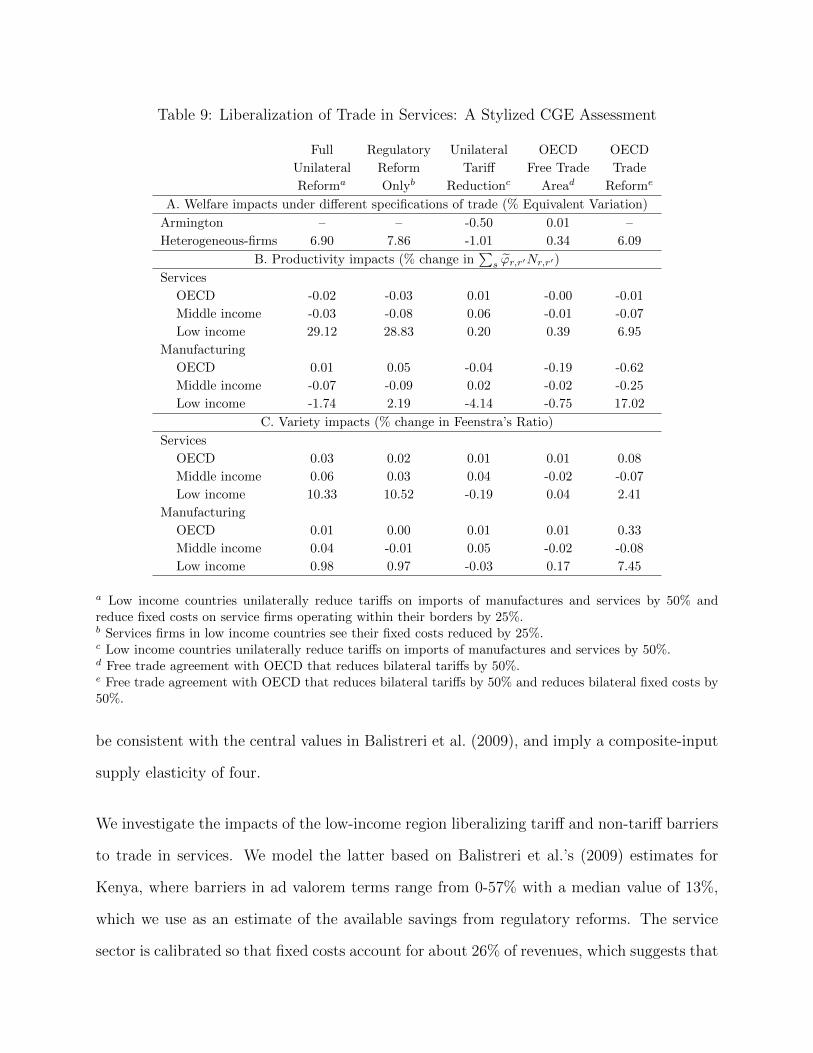
Table 9: Liberalization of Trade in Services: A Stylized CGE Assessment

Full Regulatory Unilateral OECD OECD

Unilateral Reform Tariff Free Trade Trade

Reforma Onlyb Reductionc Aread Reforme

A. Welfare impacts under different specifications of trade (% Equivalent Variation)

Armington – – -0.50 0.01 –

Heterogeneous-firms 6.90 7.86 -1.01 0.34 6.09

B. Productivity impacts (% change in∑

s ϕr,r′Nr,r′)

Services

OECD -0.02 -0.03 0.01 -0.00 -0.01

Middle income -0.03 -0.08 0.06 -0.01 -0.07

Low income 29.12 28.83 0.20 0.39 6.95

Manufacturing

OECD 0.01 0.05 -0.04 -0.19 -0.62

Middle income -0.07 -0.09 0.02 -0.02 -0.25

Low income -1.74 2.19 -4.14 -0.75 17.02

C. Variety impacts (% change in Feenstra’s Ratio)

Services

OECD 0.03 0.02 0.01 0.01 0.08

Middle income 0.06 0.03 0.04 -0.02 -0.07

Low income 10.33 10.52 -0.19 0.04 2.41

Manufacturing

OECD 0.01 0.00 0.01 0.01 0.33

Middle income 0.04 -0.01 0.05 -0.02 -0.08

Low income 0.98 0.97 -0.03 0.17 7.45

a Low income countries unilaterally reduce tariffs on imports of manufactures and services by 50% andreduce fixed costs on service firms operating within their borders by 25%.b Services firms in low income countries see their fixed costs reduced by 25%.c Low income countries unilaterally reduce tariffs on imports of manufactures and services by 50%.d Free trade agreement with OECD that reduces bilateral tariffs by 50%.e Free trade agreement with OECD that reduces bilateral tariffs by 50% and reduces bilateral fixed costs by50%.

be consistent with the central values in Balistreri et al. (2009), and imply a composite-input

supply elasticity of four.

We investigate the impacts of the low-income region liberalizing tariff and non-tariff barriers

to trade in services. We model the latter based on Balistreri et al.’s (2009) estimates for

Kenya, where barriers in ad valorem terms range from 0-57% with a median value of 13%,

which we use as an estimate of the available savings from regulatory reforms. The service

sector is calibrated so that fixed costs account for about 26% of revenues, which suggests that

a 25% reduction in these costs is roughly equivalent to a 50% reduction in regulatory barriers.

We simulate five liberalization scenarios, three which are a mix of reductions in low-income

countries’ import tariffs on services and manufactures and fixed costs for service-sector firms,

and two which simulate bilateral trade integration with the OECD. Table 9 gives details of

the scenarios, along with key model results. The first thing to note is the relative welfare im-

pact of the regulatory reform scenarios in panel A. Unilateral regulatory reform that reduces

the fixed costs of services firms in the low-income region generates a welfare gain of 7.9%. In

contrast, given optimal tariff considerations, unilateral tariff reductions lead to losses of 1%

under the heterogeneous-firms structure and 0.5% under the Armington structure. Consid-

ering bilateral policies between low-income countries and the OECD, combining 50% tariff

reductions with 50% reductions in bilateral fixed trade costs results in an 18 fold increase

in welfare gains (from 0.4% to 6%). Moreover, even in the tariff-only bilateral scenario the

heterogeneous firm model generates far larger gains than its Armington counterpart (0.01%

versus 0.39%). The heterogeneous-firm representation of trade therefore has fundamentally

important implications for measuring policy reforms. Panels B and C of Table 9 highlight

two key sources of differential economic impact: productivity shifts associated with changes

in the selection of firms into export markets on the supply side, and changes in variety

associated with the .

Unilateral regulatory reforms generate sizable productivity and variety gains for low-income

countries. We report the gains associated with new varieties of the services good, calculated

according to Feenstra’s (2010) expenditure-share based method (see Balistreri and Ruther-

ford (2012) for details). Directly interpreting the change in nh,r,r′ as an indicator of the

underlying change in varieties can be misleading because liberalization may induce the re-

placement of high-price low-quantity domestic varieties with foreign varieties. Indeed, while

the net number of varieties has been shown to decline with trade costs (Baldwin and Forslid,

2010; Feenstra, 2010), this does not by itself indicate a gain or loss as each variety has a

different price.

We close this section by emphasizing that our simulations rely on a set of parameters not

commonly used by CGE models. In particular, the values of shape parameter on the dis-

tribution of firm productivities and the bilateral fixed costs of trade are drawn from the

structural estimation procedures developed in Balistreri et al. (2011). It has traditionally

been the case that these sorts of parameters are estimated using econometric models that are

divorced from broader theory of general equilibrium or its particular algebraic elaboration in

the numerical simulation to be parameterized. By contrast, structural estimation techniques

bring econometric and numerical simulation modeling together in a consistent fashion by

imposing theory-based restrictions on the values of estimated parameters. An important

example is Anderson and van Wincoop’s (2003) widely cited study, whose welfare impacts

have been shown to be inconsistent with its estimation procedure unless the latter is prop-

erly constrained by restrictions based on the conditions of general equilibrium (Balistreri

and Hillberry, 2008, 2007).

Structural estimation of the parameters of our heterogeneous-firm model proceeds by iso-

lating the complementarity conditions that characterize the trade equilibrium and imposing

these as a set of constraints on econometric estimation. Following Balistreri et al. (2011),

consider a vector-valued function that specifies the equilibrium in bilateral trade markets

conditional on the observed benchmark demand for the regional domestic-import compos-

ites, qAh,r, and the domestic supply of the traded good, yh,r. The system of equations may

be stacked to generate the vector-valued function Ξ(V ,Γ) = 0 which implicitly maps the

vector of parameters, Γ, to the vector of endogenous variables, V . The key parameters to be

estimated are the Pareto shape coefficient and the bilateral fixed costs of trade, a,FOh,r,r′ ∈ Γ,

while the endogenous variable that we are interested in reproducing is the value of bilateral

trade, qHh,r,r′ pHh,r,r′nh,r,r′ ∈ V . Using V to denote the corresponding vector of observations

of the variables, we can find the best estimates of the parameters by solving the nonlinear

program:

minΓ,V

(V − V

)2∣∣∣∣Ξ(V , Γ,Γ?) = 0,Γ? = K

where Γ? are a set of assumed parameters and K is a vector of constants.

This methodology has an appealing general applicability, but in practice it is severely con-

strained by the degrees of freedom offered by the data, which permit only a limited number

of structural parameters to be estimated. For example, in their central case, Balistreri et al.

(2011) only estimate the Pareto shape parameter and fixed trade costs. Furthermore, the

structure of bilateral fixed costs is such that only each region’s vectors of aggregate inward

and outward costs can be estimated, not the full bilateral matrix. Notwithstanding these

shortcomings, the need to link CGE models’ structural representations of the economy to

underlying empirically-determined parameters will likely mean that structural estimation

will continue to be an area of active research in the foreseeable future.

5 CONCLUSIONS

This chapter documents contemporary Computable General Equilibrium (CGE) approaches

to policy evaluation. The algebraic formulation of a canonical multiregion model of world

trade and production is presented. This standard class of models is widely employed in

the study of economic integration and climate policy. The standard model is extended to

consider specific advances in CGE research. First, the incorporation of detailed process-level

production technologies are shown using bottom-up techniques. These techniques enhance

models that consider energy systems. It is especially popular in climate change mitigation

research, where it allows CGE models to credibly represent the impacts of policy on fuel and

alternative energy use.

In the context of trade policy the canonical model is extended using a trade structure that is

currently favored by many trade theorists. The model consider services and manufacturing

firms providing differentiated products and engaged in monopolistic competition. Critical to

this new theory is the selection of firms with different productivities (heterogeneous firms)

into different national markets. This extension illustrates important margins for the gains

from trade, that are not apparent in the standard model. In particular, there are variety

effects as the number and composition of available goods and services change with policy. In

addition, firm heterogeneity indicates that resource reallocation within an industry toward

more productive firms can boost overall productivity.

The model formulations presented offer an illustrative guide and documentation of contem-

porary CGE applications. While technically advanced, these models offer the same advan-

tages for policy evaluation that have been the hallmark of CGE models over the past three

decades. The rigorous theoretic structure allows for an investigation of the drivers behind

specific outcomes, and the sensitivity of specific outcomes to alternative assumptions. Ex-

amples presented here are useful for practitioners interested in advanced and alternative

techniques and as a guide to understanding the model interactions present in many contem-

porary analyses.

Notes

1Jorgenson and Wilcoxen (1993); Bye (2000); Bovenberg and Goulder (2001); Balistreri (2002); Diao et al.

(2005); Bovenberg et al. (2005); Dellink (2005); Otto et al. (2007); Otto and Reilly (2008); Otto et al. (2008).

2(Bernstein et al., 1999; Diao et al., 2003; Babiker et al., 2009; Ross et al., 2009; Tuladhar et al., 2009).

3Jean et al. (2014); Aydin and Acar (2010); Missaglia and Valensisi (2014); Engelbert et al. (2014);

Braymen (2011); Kawai and Zhai (2009); Lee et al. (2009); Chao et al. (2006); Lee et al. (2004); Georges

et al. (2013); Bout et al. (2012); Gouel et al. (2011); Winchester (2009); Ghosh and Rao (2010); Brockmeier

and Pelikan (2008); Ariyasajjakorn et al. (2009); Ghosh and Rao (2005); Francois et al. (2005); Lee and

van der Mensbrugghe (2004); Flaig et al. (2013); Perali et al. (2012); Kitwiwattanachai et al. (2010); Bajo-

Rubio and Gmez-Plana (2005).

4lvarez Martinez and Polo (2012); von Arnim (2009).

5Kleinwechter and Grethe (2012); Naranpanawa et al. (2011); Pauw and Thurlow (2011); Gumilang et al.

(2011); Mabugu and Chitiga (2009); Acharya and Cohen (2008); Abbott et al. (2009); O’Ryan et al. (2005);

Mirza et al. (2014); Hertel and Zhai (2006); Chan et al. (2005); Naude and Coetzee (2004).

6Solaymani and Kari (2013); Naranpanawa and Bandara (2012); AlShehabi (2012); Dartanto (2013);

Arndt et al. (2011); Scaramucci et al. (2006).

7Aglietta et al. (2007); Creedy and Guest (2008); Fougre et al. (2007); Rausch and Rutherford (2010);

Lisenkova et al. (2013); Wright (2013).

8Radulescu and Stimmelmayr (2010); Toh and Lin (2005); Field and Wongwatanasin (2007); Giesecke

and Nhi (2010); Boeters (2013); Mabugu et al. (2013).

9Al Shehabi (2013); Bjertnaes (2011); He et al. (2014); Jiang and Lin (2014); Sancho (2010); Liu and Li

(2011); Akkemik and Oguz (2011); Lin and Jiang (2011); Vandyck and Regemorter (2014); Solaymani and

Kari (2014); He et al. (2011).

10Santos et al. (2013); Allan et al. (2008); Hanley et al. (2009); Bjertaes and Fhn (2008); Shi et al. (2009);

O’Neill et al. (2012).

11Allan et al. (2007); Anson and Turner (2009); Turner and Hanley (2011); Martinsen (2011); Lu et al.

(2010); Otto et al. (2007); Parrado and Cian (2014); Dimitropoulos (2007); Lecca et al. (2014); Turner (2009).

12Timilsina et al. (2011, 2013); Bae and Cho (2010); Proenca and Aubyn (2013); Cansino et al. (2013, 2014);

Hoefnagels et al. (2013); Boehringer et al. (2013); Arndt et al. (2012); Gunatilake et al. (2014); Wianwiwat

and Asafu-Adjaye (2013); Doumax et al. (2014); Ge et al. (2014); Trink et al. (2010); Kretschmer and

Peterson (2010).

13Kallbekken and Westskog (2005); Klepper and Peterson (2005); Nijkamp et al. (2005); Bohringer and

Welsch (2004); Bohringer and Helm (2008); Kallbekken and Rive (2007); Calvin et al. (2009); Magne et al.

(2014).

14Klepper and Peterson (2006); Bohringer et al. (2007); Kasahara et al. (2007); Telli et al. (2008); Thepkhun

et al. (2013); Hermeling et al. (2013); Orlov and Grethe (2012); Hubler et al. (2014); Lu et al. (2010); Lim

(2011); Liang et al. (2007); Loisel (2009); Wang et al. (2009); Dai et al. (2011); Hubler (2011); Meng et al.

(2013).

15Bovenberg et al. (2005, 2008); Rose and Oladosu (2002); van Heerden et al. (2006); Oladosu and Rose

(2007); Ojha (2009).

16Bor and Huang (2010); Fraser and Waschik (2013); Allan et al. (2014); Boeters (2014); Dissou and

Siddiqui (2014).

17McCarl and Sands (2007); Glomsrod et al. (2011); Michetti and Rosa (2012); Bohringer et al. (2014).

18Babiker (2005); Babiker and Rutherford (2005); Ghosh et al. (2012); Bao et al. (2013); Branger and

Quirion (2014); Hubler (2012); Alexeeva-Talebi et al. (2012); Bohringer et al. (2012); Weitzel et al. (2012);

Lanzi et al. (2012); Boeters and Bollen (2012); Caron (2012); Turner et al. (2012); Kuik and Hofkes (2010);

Bruvoll and Faehn (2006); Jakob et al. (2013); Egger and Nigai (2014).

19Viguier et al. (2006); Otto et al. (2007); Fisher-Vanden and Ho (2007); Fisher-Vanden and Sue Wing

(2008); Peretto (2008); Mahmood and Marpaung (2014); Sue Wing and Eckaus (2007); Jin (2012); Qi et al.

(2014); Bretschger et al. (2011); Heggedal and Jacobsen (2011).

20Hagem et al. (2006); Maisonnave et al. (2012); Daenzer et al. (2014).

21Schafer and Jacoby (2005); McFarland et al. (2004); Jacoby et al. (2006); Berg (2007); Qi et al. (2014);

Okagawa et al. (2012); van den Broek et al. (2011); Karplus et al. (2013b,a); Kretschmer et al. (2009);

Glomsrod and Taoyuan (2005); Timilsina et al. (2011); Timilsina and Mevel (2013); Sands et al. (2014).

22Examples of the latter are MARKAL (Schafer and Jacoby, 2005), and economic dispatch or capacity

expansion models of the electric power sector (Lanz and Rausch, 2011).

23 Theoretical models make the simplifying assumption that variable trade and transport costs are incurred

as a loss of product as the product moves through space—iceberg melt. This is generally inappropriate in

CGE models, which must be consistent with transport services payments and government revenues from

tariffs and other trade distortions recorded in their calibration dataset. We introduce Ch,r,r′ , however,

because it serves as an important unobserved-trade-cost parameter that facilitates a calibration of the model

under symmetric demand across all varieties. Like the coefficients ξi,r and κt,i,r′,r in the canonical model, the

values of Ch,r,r′ are fixed such that the model replicates the trade equilibrium in the benchmark. See Balistreri

and Rutherford (2012) for in-depth discussion of the equivalence between calibrating the heterogeneous firms

model using idiosyncratic demand biases versus unobserved trade costs.

24 Numerical results are typically not sensitive to the scale and distribution of benchmark fixed costs

because only the value of the elasticity parameter determines the markup over marginal cost. Assumptions

about fixed operating costs simply scale our measure of the number of firms: the larger the assumed values

of FOh,r,r′ , the larger the implied per-firm revenue, and, with a given value of trade, the smaller the calibrated

initial number of firms.

REFERENCES

Abbott, P., J. Bentzen, and F. Tarp (2009). Trade and development: Lessons from Vietnam’s

past trade agreements. World Development 37 (2), 341–353.

Acharya, S. and S. Cohen (2008). Trade liberalisation and household welfare in Nepal.

Journal of Policy Modeling 30 (6), 1057–1060.

Adkins, L. C., D. S. Rickman, and A. Hameed (2003). Bayesian estimation of regional

production for CGE modeling. Journal of Regional Science 43, 641–661.

Aglietta, M., J. Chateau, J. Fayolle, M. Juillard, J. L. Cacheux, G. L. Garrec, and V. Touz

(2007). Pension reforms in Europe: An investigation with a computable OLG world model.

Economic Modelling 24 (3), 481–505.

Ahmed, N. and J. H. Peerlings (2009). Addressing workers rights in the textile and apparel

industries: Consequences for the Bangladesh economy. World Development 37 (3), 661–

675.

Akkemik, K. A. and F. Oguz (2011). Regulation, efficiency and equilibrium: A general

equilibrium analysis of liberalization in the Turkish electricity market. Energy 36 (5),

3282–3292.

Al Shehabi, O. H. (2013). Modelling energy and labour linkages: A CGE approach with an

application to Iran. Economic Modelling 35, 88–98.

Alexeeva-Talebi, V., C. Bohringer, A. Loschel, and S. Voigt (2012). The value-added of sec-

toral disaggregation: Implications on competitive consequences of climate change policies.

Energy Economics 34, Supplement 2, S127–S142.

Allan, G., N. Hanley, P. McGregor, K. Swales, and K. Turner (2007). The impact of increased

efficiency in the industrial use of energy: A computable general equilibrium analysis for

the United Kingdom. Energy Economics 29 (4), 779–798.

Allan, G., P. Lecca, P. McGregor, and K. Swales (2014). The economic and environmental

impact of a carbon tax for Scotland: A computable general equilibrium analysis. Ecological

Economics 100, 40–50.

Allan, G. J., I. Bryden, P. G. McGregor, T. Stallard, J. K. Swales, K. Turner, and R. Wallace

(2008). Concurrent and legacy economic and environmental impacts from establishing a

marine energy sector in Scotland. Energy Policy 36 (7), 2734–2753.

AlShehabi, O. H. (2012). Energy and labour reform: Evidence from Iran. Journal of Policy

Modeling 34 (3), 441–459.

Amelung, B. and A. Moreno (2012). Costing the impact of climate change on tourism in

europe: results of the PESETA project. Climatic Change 112, 83–100.

Anderson, J. E. and E. van Wincoop (2003, March). Gravity with gravitas: A solution to

the border puzzle. American Economic Review 93 (1), 170–192.

Anson, S. and K. Turner (2009). Rebound and disinvestment effects in refined oil consump-

tion and supply resulting from an increase in energy efficiency in the Scottish commercial

transport sector. Energy Policy 37 (9), 3608–3620.

Ariyasajjakorn, D., J. P. Gander, S. Ratanakomut, and S. E. Reynolds (2009). ASEAN FTA,

distribution of income, and globalization. Journal of Asian Economics 20 (3), 327–335.

Armington, P. (1969). A theory of demand for products distinguished by place of production.

International Monetary Fund Staff Papers XVI, 159–78.

Arndt, C., R. Benfica, and J. Thurlow (2011). Gender implications of biofuels expansion in

Africa: The case of Mozambique. World Development 39 (9), 1649–1662.

Arndt, C., K. Pauw, and J. Thurlow (2012). Biofuels and economic development: A com-

putable general equilibrium analysis for Tanzania. Energy Economics 34 (6), 1922–1930.

Arndt, C., S. Robinson, and F. Tarp (2002). Parameter estimation for a computable general

equilibrium model: a maximum entropy approach. Economic Modelling 19, 375–398.

Auriol, E. and M. Warlters (2012). The marginal cost of public funds and tax reform in

Africa. Journal of Development Economics 97 (1), 58 – 72.

Aydin, L. and M. Acar (2010). Economic and environmental implications of Turkish accession

to the european union: A CGE analysis. Energy Policy 38 (11), 7031–7040.

Aydin, L. and M. Acar (2011). Economic impact of oil price shocks on the Turkish economy

in the coming decades: A dynamic CGE analysis. Energy Policy 39 (3), 1722–1731.

Babiker, M., A. Gurgel, S. Paltsev, and J. Reilly (2009). Forward-looking versus recursive-

dynamic modeling in climate policy analysis: A comparison. Economic Modelling 26 (6),

1341–1354.

Babiker, M. H. (2005). Climate change policy, market structure, and carbon leakage. Journal

of International Economics 65, 421–445.

Babiker, M. H. and T. F. Rutherford (2005). The economic effects of border measures in

subglobal climate agreements. Energy Journal 26, 99–125.

Bae, J. H. and G.-L. Cho (2010). A dynamic general equilibrium analysis on fostering a

hydrogen economy in Korea. Energy Economics 32, Supplement 1, S57–S66.

Bajo-Rubio, O. and A. G. Gmez-Plana (2005). Simulating the effects of the European single

market: A CGE analysis for Spain. Journal of Policy Modeling 27 (6), 689–709.

Baldwin, R. E. and R. Forslid (2010). Trade liberalization with heterogeneous firms. Review

of Development Economics 14 (2), 161–176.

Balistreri, E. J. (2002). Operationalizing equilibrium unemployment: A general equilibrium

external economies approach. Journal of Economic Dynamics and Control 26 (3), 347–374.

Balistreri, E. J. and R. H. Hillberry (2007). Structural estimation and the border puzzle.

Journal of International Economics 72 (2), 451–463.

Balistreri, E. J. and R. H. Hillberry (2008). The gravity model: An illustration of structural

estimation as calibration. Economic Inquiry 46 (4), 511–527.

Balistreri, E. J., R. H. Hillberry, and T. F. Rutherford (2010). Trade and welfare: Does

industrial organization matter? Economics Letters 109 (2), 85–87.

Balistreri, E. J., R. H. Hillberry, and T. F. Rutherford (2011). Structural estimation and

solution of international trade models with heterogeneous firms. Journal of International

Economics 83 (2), 95–108.

Balistreri, E. J. and T. F. Rutherford (2012). Computing general equilibrium theories of

monopolistic competition and heterogeneous firms. In P. B. Dixon and D. W. Jorgenson

(Eds.), Handbook of Computable General Equilibrium Modeling. Amsterdam: Elsevier.

Balistreri, E. J., T. F. Rutherford, and D. G. Tarr (2009). Modeling services liberalization:

The case of Kenya. Economic Modelling 26 (3), 668–679.

Ballard, C. L. and D. Fullerton (1992). Distortionary taxes and the provision of public goods.

Journal of Economic Perspectives 6 (3), 117–131.

Bao, Q., L. Tang, Z. Zhang, and S. Wang (2013). Impacts of border carbon adjustments on

China’s sectoral emissions: Simulations with a dynamic computable general equilibrium

model. China Economic Review 24, 77–94.

Barkhordar, Z. A. and Y. Saboohi (2013). Assessing alternative options for allocating oil

revenue in Iran. Energy Policy 63, 1207–1216.

Bartelsman, E. J. and M. Doms (2000). Understanding productivity: Lessons from longitu-

dinal microdata. Journal of Economic Literature 38 (3), 569–594.

Beckman, J., T. Hertel, and W. Tyner (2011). Validating energy-oriented CGE models.

Energy Economics 33 (5), 799–806.

Berg, C. (2007). Household transport demand in a CGE-framework. Environmental and

Resource Economics 37, 573–597.

Bernard, A., J. Jensen, and P. Schott (2006). Trade costs, firms and productivity. Journal

of monetary Economics 53 (5), 917–937.

Bernard, A. B., J. Eaton, J. B. Jensen, and S. Kortum (2003). Plants and productivity in

international trade. The American Economic Review 93 (4), pp. 1268–1290.

Bernard, A. B. and J. B. Jensen (1999). Exceptional exporter performance: Cause, effect,

or both? Journal of International Economics 47 (1), 1–25.

Bernstein, P., W. Montgomery, T. Rutherford, and G. Yang (1999). Global impacts of the

kyoto agreement: results from the MS-MRT model. Resource and Energy Economics 21,

375–413.

Berrittella, M., A. Bigano, R. Roson, and R. Tol (2006). A general equilibrium analysis of

climate change impacts on tourism. Tourism Management 25, 913–924.

Bigano, A., F. Bosello, R. Roson, and R. Tol (2008). Economy-wide impacts of climate

change: a joint analysis for sea level rise and tourism. Mitigation and Adaptation Strategies

for Global Change 13, 765–791.

Bigano, A., J. Hamilton, and R. Tol (2007). The impact of climate change on domestic and

international tourism: A simulation study. Integrated Assessment Journal 7, 25–29.

Bjertaes, G. H. and T. Fhn (2008). Energy taxation in a small, open economy: Social

efficiency gains versus industrial concerns. Energy Economics 30 (4), 2050–2071.

Bjertnaes, G. H. (2011). Avoiding adverse employment effects from electricity taxation in

Norway: What does it cost? Energy Policy 39 (9), 4766–4773.

Boehringer, C., A. Keller, and E. van der Werf (2013). Are green hopes too rosy? employment

and welfare impacts of renewable energy promotion. Energy Economics 36, 277–285.

Boeters, S. (2013). Optimal tax progressivity in unionised labour markets: Simulation results

for Germany. Computational Economics 41, 447–474.

Boeters, S. (2014). Optimally differentiated carbon prices for unilateral climate policy. En-

ergy Economics , in press.

Boeters, S. and J. Bollen (2012). Fossil fuel supply, leakage and the effectiveness of border

measures in climate policy. Energy Economics 34, Supplement 2, S181–S189.

Bohringer, C. (1998). The synthesis of bottom-up and top-down in energy policy modeling.

Energy Economics 20, 233–248.

Bohringer, C., B. Bye, T. Fhn, and K. E. Rosendahl (2012). Alternative designs for tariffs on

embodied carbon: A global cost-effectiveness analysis. Energy Economics 34, Supplement

2, S143–S153.

Bohringer, C. and C. Helm (2008). On the fair division of greenhouse gas abatement cost.

Resource and Energy Economics 30 (2), 260–276.

Bohringer, C., U. Moslener, and B. Sturm (2007). Hot air for sale: a quantitative assess-

ment of Russia’s near-term climate policy options. Environmental and Resource Eco-

nomics 38 (4), 545–572.

Bohringer, C. and T. F. Rutherford (2008). Combining bottom-up and top-down. Energy

Economics 30, 574–596.

Bohringer, C. and T. F. Rutherford (2009). Integrated assessment of energy policies: De-

composing top-down and bottom-up. Journal of Economic Dynamics and Control 33,

1648–1661.

Bohringer, C., T. F. Rutherford, and M. Springmann (2014). Clean-development invest-

ments: An incentive-compatible CGE modelling framework. Environmental and Resource

Economics , in press.

Bohringer, C. and H. Welsch (2004). Contraction and convergence of carbon emissions: an

intertemporal multi-region CGE analysis. Journal of Policy Modeling 26 (1), 21–39.

Bondeau, A., P. Smith, A. Zaehle, S. Schaphoff, W. Lucht, W. Cramer, D. Gerten, H. Lotze-

Campen, C. Muller, M. Reichstein, and B. Smith (2007). Modeling the role of agriculture

for the 20th century global terrestrial carbon balance. Global Change Biology 13, 679–706.

Bor, Y. J., Y.-C. Chuang, W.-W. Lai, and C.-M. Yang (2010). A dynamic general equilibrium

model for public R&D investment in Taiwan. Economic Modelling 27 (1), 171–183.

Bor, Y. J. and Y. Huang (2010). Energy taxation and the double dividend effect in Tai-

wan’s energy conservation policyan empirical study using a computable general equilibrium

model. Energy Policy 38 (5), 2086–2100.

Bosello, F., C. Carraro, and E. D. Cian (2010a). An analysis of adaptation as a response to

climate change. In B. Lomborg (Ed.), Smart Solutions to Climate Change, pp. 222–276.

Cambridge: Cambridge University Press.

Bosello, F., C. Carraro, and E. D. Cian (2010b). Climate policy and the optimal balance be-

tween mitigation, adaptation and unavoided damage. FEEM Working Paper No. 32.2010,

Fondazione Eni Enrico Mattei.

Bosello, F., E. D. Cian, and R. Roson (2007). Climate change, energy demand and market

power in a general equilibrium model of the world economy. FEEM Working Paper No.

71.2007, Fondazione Eni Enrico Mattei.

Bosello, F., F. Eboli, and R. Pierfederici (2012). Assessing the economic im-

pacts of climate change. Review of Environment, Energy and Economics

(Re3) http://dx.doi.org/10.7711/feemre3.2012.02.002.

Bosello, F., R. Nicholls, J. Richards, R. Roson, and R. Tol (2012). Economic impacts of

climate change in Europe: sea-level rise. Climatic Change 112, 63–81.

Bosello, F., R. Roson, and R. Tol (2006). Economy wide estimates of the implications of

climate change: Human health. Ecological Economics 58, 579–591.

Bosello, F., R. Roson, and R. Tol (2007). Economy wide estimates of the implications of

climate change: Sea-level rise. Environmental and Resource Economics 37, 549–571.

Bosello, F. and J. Zhang (2006). Gli effetti del cambiamento climatico in agricoltura. Ques-

tione Agraria 1-2006, 97–124.

Boussard, J.-M., F. Grard, M. G. Piketty, M. Ayouz, and T. Voituriez (2006). Endoge-

nous risk and long run effects of liberalization in a global analysis framework. Economic

Modelling 23 (3), 457–475.

Bout, A., V. Berisha-Krasniqi, C. Estrades, and D. Laborde (2012). Trade and investment

in Latin America and Asia: Perspectives from further integration. Journal of Policy

Modeling 34 (2), 193–210.

Bovenberg, A. L. and L. H. Goulder (2001). Neutralizing the adverse industry impacts of

CO2 abatement policies: What does it cost? In C. Carraro and G. E. Metcalf (Eds.),

Behavioral and Distributional Effects of Environmental Policy, pp. 45–90. Chicago, IL:

University of Chicago Press.

Bovenberg, A. L., L. H. Goulder, and D. J. Gurney (2005). Efficiency costs of meeting

industry-distributional constraints under environmental permits and taxes. RAND Journal

of Economics 36, 950–970.

Bovenberg, A. L., L. H. Goulder, and M. R. Jacobsen (2008). Costs of alternative environ-

mental policy instruments in the presence of industry compensation requirements. Journal

of Public Economics 92 (5-6), 1236–1253.

Branger, F. and P. Quirion (2014). Would border carbon adjustments prevent carbon leak-

age and heavy industry competitiveness losses? insights from a meta-analysis of recent

economic studies. Ecological Economics 99, 29–39.

Braymen, C. B. (2011). Sectoral structure, heterogeneous plants, and international trade.

Economic Modelling 28 (4), 1967–1976.

Breisinger, C., X. Diao, and J. Thurlow (2009). Modeling growth options and structural

change to reach middle income country status: The case of Ghana. Economic Mod-

elling 26 (2), 514–525.

Bretschger, L., R. Ramer, and F. Schwark (2011). Growth effects of carbon policies: Ap-

plying a fully dynamic CGE model with heterogeneous capital. Resource and Energy

Economics 33 (4), 963–980.

Bretschger, L. and S. Smulders (2011). Technologies, preferences, and policies for a sustain-

able use of natural resources. Resource and Energy Economics 33 (4), 881–892.

Brockmeier, M. and J. Pelikan (2008). Agricultural market access: A moving target in the

WTO negotiations? Food Policy 33 (3), 250–259.

Bruvoll, A. and T. Faehn (2006). Transboundary effects of environmental policy: Markets

and emission leakages. Ecological Economics 59 (4), 499–510.

Bye, B. (2000). Environmental tax reform and producer foresight: An intertemporal com-

putable general equilibrium analysis. Journal of Policy Modeling 22, 719–752.

Calvin, K., P. Patel, A. Fawcett, L. Clarke, K. Fisher-Vanden, J. Edmonds, S. H. Kim,

R. Sands, and M. Wise (2009). The distribution and magnitude of emissions mitigation

costs in climate stabilization under less than perfect international cooperation: SGM

results. Energy Economics 31, Supplement 2, S187–S197.

Cansino, J., M. Cardenete, J. Gonzlez-Limn, and R. Romn (2013). Economic impacts of

biofuels deployment in Andalusia. Renewable and Sustainable Energy Reviews 27, 274–282.

Cansino, J., M. Cardenete, J. Gonzlez-Limn, and R. Romn (2014). The economic influ-

ence of photovoltaic technology on electricity generation: A CGE (computable general

equilibrium) approach for the Andalusian case. Energy , in press.

Capros, P., T. Georgakopoulos, D. Van Regemorter, S. Proost, T. Schmidt, and K. Conrad

(1997). European union: the GEM-E3 general equilibrium model. Economic and Financial

Modelling 4, 51–160.

Caron, J. (2012). Estimating carbon leakage and the efficiency of border adjustments in gen-

eral equilibrium—does sectoral aggregation matter? Energy Economics 34, Supplement

2, S111–S126.

Chan, N., T. K. Dung, M. Ghosh, and J. Whalley (2005). Adjustment costs in labour

markets and the distributional effects of trade liberalization: Analytics and calculations

for Vietnam. Journal of Policy Modeling 27 (9), 1009–1024.

Chao, C.-C., E. S. YU, and W. YU (2006). China’s import duty drawback and VAT rebate

policies: A general equilibrium analysis. China Economic Review 17 (4), 432–448.

Chen, Y., J. Reilly, and S. Paltsev (2011). The prospects for coal-to-liquid conversion: A

general equilibrium analysis. Energy Policy 39 (9), 4713–4725.

Ciscar, J., A. Iglesias, L. Feyen, L. Szabo, D. Van Regemorter, B. Amelunge, R. Nicholls,

P. Watkiss, O. Christensen, R. Dankers, L. Garrote, C. M. Goodess, A. Hunt, A. Moreno,

J. Richards, and A. Soria (2011). Physical and economic consequences of climate change

in Europe. Proceedings of the National Academy of Sciences 108, 2678–2683.

Ciscar, J., A. Soria, C. Goodess, O. Christensen, A. Iglesias, L. Garrote, M. Moneo,

S. Quiroga, L. Feyen, R. Dankers, R. Nicholls, J. Richards, R. R. F. Bosello, B. Amelung,

A. Moreno, P. Watkiss, A. Hunt, S. Pye, L. Horrocks, L. Szabo, and D. van Rege-

morter (2009). Climate change impacts in europe, final report of the PESETA research

project. Working Paper No. JRC55391, European Union Joint Research Centre Institute

for Prospective and Technological Studies.

Ciscar, J., L. Szabo, D. van Regemorter, and A. Soria (2012). The integration of PESETA

sectoral economic impacts into the GEM-E3 europe model: methodology and results.

Climatic Change 112, 127–142.

Clausen, V. and H. Schrenberg-Frosch (2012). Aid, spending strategies and productivity

effects: A multi-sectoral CGE analysis for Zambia. Economic Modelling 29 (6), 2254–

2268.

Creedy, J. and R. Guest (2008). Changes in the taxation of private pensions: Macroeconomic

and welfare effects. Journal of Policy Modeling 30 (5), 693–712.

Daenzer, K., I. Sue Wing, and K. Fisher-Vanden (2014). Coal’s medium-run future under

atmospheric greenhouse gas stabilization. Climatic Change 123, 763–783.

Dahlby, B. (2008). The Marginal Cost of Public Funds. Cambridge, MA: MIT Press.

Dai, H., T. Masui, Y. Matsuoka, and S. Fujimori (2011). Assessment of China’s climate

commitment and non-fossil energy plan towards 2020 using hybrid AIM/CGE model.

Energy Policy 39 (5), 2875–2887.

Dartanto, T. (2013). Reducing fuel subsidies and the implication on fiscal balance and

poverty in Indonesia: A simulation analysis. Energy Policy 58, 117–134.

Darwin, R., , and R. Tol (2001). Estimates of the economic effects of sea level rise. Envi-

ronmental and Resource Economics 19, 113–129.

Darwin, R. (1999). A FARMer’s view of the Ricardian approach to measuring effects of

climatic change on agriculture. Climatic Change 41, 371–411.

Darwin, R., M. Tsigas, J. Lewabdrowski, and A. Raneses (1995). World agriculture and cli-

mate change. Agricultural Economic Report No. 703, U.S. Dept. of Agriculture, Economic

Research Service.

De Cian, E., E. Lanzi, and R. Roson (2013). Seasonal temperature variations and energy

demand: A panel cointegration analysis for climate change impact assessment. Climatic

Change 116, 805–825.

Debowicz, D. and J. Golan (2014). The impact of oportunidades on human capital and

income distribution in mexico: A top-down/bottom-up approach. Journal of Policy Mod-

eling 36 (1), 24–42.

Deke, O., K. Hooss, C. Kasten, G. Klepper, and K. Springer (2001). Economic impact of

climate change: Simulations with a regionalized climate-economy model. Working Paper

No. 1065, Kiel Institute for the World Economy.

Dell, M., B. F. Jones, and B. A. Olken (2014). What Do We Learn from the Weather? The

New Climate-Economy Literature. Journal of Economic Literature 52, 740–798.

Dellink, R. B. (2005). Modelling the costs of environmental policy: a dynamic applied general

equilibrium assessment. Cheltenham: Edward Elgar.

Deng, Z., R. Falvey, and A. Blake (2012). Trading market access for technology? tax

incentives, foreign direct investment and productivity spillovers in China. Journal of

Policy Modeling 34 (5), 675–690.

Diao, X., S. Fan, and X. Zhang (2003). China’s WTO accession: impacts on regional

agricultural income—a multi-region, general equilibrium analysis. Journal of Comparative

Economics 31, 332–351.

Diao, X., J. Rattso, and H. E. Stokke (2005). International spillovers, productivity growth

and openness in Thailand: an intertemporal general equilibrium analysis. Journal of

Development Economics 76, 429–450.

Dimitropoulos, J. (2007). Energy productivity improvements and the rebound effect: An

overview of the state of knowledge. Energy Policy 35 (12), 6354–6363.

Dissou, Y. and M. S. Siddiqui (2014). Can carbon taxes be progressive? Energy Eco-

nomics 42, 88–100.

Dixon, P., B. Lee, T. Muehlenbeck, M. T. Rimmer, A. Z. Rose, and G. Verikios (2010).

Effects on the U.S. of an H1N1 epidemic: Analysis with a quarterly CGE model. Journal

of Homeland Security and Emergency Management 7, art. 75.

Djiofack, C. Z. and L. D. Omgba (2011). Oil depletion and development in Cameroon: A

critical appraisal of the permanent income hypothesis. Energy Policy 39 (11), 7202–7216.

Doumax, V., J.-M. Philip, and C. Sarasa (2014). Biofuels, tax policies and oil prices in

France: Insights from a dynamic CGE model. Energy Policy 66, 603–614.

Eboli, F., R. Parrado, and R. Roson (2010). Climate-change feedback on economic growth:

explorations with a dynamic general equilibrium model. Environment and Development

Economics 15, 515–533.

Egger, P. and S. Nigai (2014). Energy demand and trade in general equilibrium. Environ-

mental and Resource Economics , in press.

Engelbert, T., B. Bektasoglu, and M. Brockmeier (2014). Moving toward the EU or the

Middle East? an assessment of alternative Turkish foreign policies utilizing the GTAP

framework. Food Policy 47, 46–61.

Feenstra, R. C. (2010). Measuring the gains from trade under monopolistic competition.

Canadian Journal of Economics 43 (1), 1–28.

Femenia, F. and A. Gohin (2011). Dynamic modelling of agricultural policies: The role of

expectation schemes. Economic Modelling 28 (4), 1950–1958.

Feyen, L., R. Dankers, K. Bodis, P. Salamon, and J. Barredo (2012). Fluvial flood risk in

Europe in present and future climates. Climatic Change 112, 47–62.

Field, A. J. and U. Wongwatanasin (2007). Tax policies impact on output, trade and income

in Thailand. Journal of Policy Modeling 29 (3), 361–380.

Fisher-Vanden, K. and M. Ho (2010). Technology, development and the environment. Journal

of Environmental Economics and Management 59, 94–108.

Fisher-Vanden, K. and M. S. Ho (2007). How do market reforms affect China’s responsiveness

to environmental policy? Journal of Development Economics 82, 200–233.

Fisher-Vanden, K. and I. Sue Wing (2008). Accounting for quality: Issues with modeling

the impact of R&D on economic growth and carbon emissions in developing economies.

Energy Economics 30, 2771–2784.

Flaig, D., O. Rubin, and K. Siddig (2013). Imperfect competition, border protection and

consumer boycott: The future of the dairy industry in Israel. Journal of Policy Model-

ing 35 (5), 838–851.

Fougre, M., J. Mercenier, and M. Mrette (2007). A sectoral and occupational analysis

of population ageing in Canada using a dynamic CGE overlapping generations model.

Economic Modelling 24 (4), 690–711.

Francois, J. F., M. McQueen, and G. Wignaraja (2005). European Union-developing country

FTAs: overview and analysis. World Development 33 (10), 1545–1565.

Fraser, I. and R. Waschik (2013). The double dividend hypothesis in a CGE model: Specific

factors and the carbon base. Energy Economics 39, 283–295.

Fugazza, M. and J.-C. Maur (2008). Non-tariff barriers in CGE models: How useful for

policy? Journal of Policy Modeling 30, 475–490.

Fullerton, D. and D. L. Rogers (1993). Who Bears the Lifetime Tax Burden? Washington,

DC: Brookings Institution.

Ge, J., Y. Lei, and S. Tokunaga (2014). Non-grain fuel ethanol expansion and its effects on

food security: Acomputable general equilibrium analysis for China. Energy 65, 346–356.

Georges, P., K. Lisenkova, and M. Mrette (2013). Can the ageing North benefit from ex-

panding trade with the South? Economic Modelling 35, 990–998.

Ghosh, M., D. Luo, M. S. Siddiqui, and Y. Zhu (2012). Border tax adjustments in the climate

policy context: CO2 versus broad-based GHG emission targeting. Energy Economics 34,

Supplement 2, S154–S167.

Ghosh, M. and S. Rao (2005). A Canada-U.S. customs union: Potential economic impacts

in NAFTA countries. Journal of Policy Modeling 27 (7), 805–827.

Ghosh, M. and S. Rao (2010). Chinese accession to the WTO: Economic implications for

China, other Asian and North American economies. Journal of Policy Modeling 32 (3),

389–398.

Giesecke, J. A. and T. H. Nhi (2010). Modelling value-added tax in the presence of multi-

production and differentiated exemptions. Journal of Asian Economics 21 (2), 156–173.

Glomsrod, S. and W. Taoyuan (2005). Coal cleaning: a viable strategy for reduced carbon

emissions and improved environment in China? Energy Policy 33 (4), 525–542.

Glomsrod, S., T. Wei, G. Liu, and J. B. Aune (2011). How well do tree plantations comply

with the twin targets of the clean development mechanism? the case of tree plantations

in Tanzania. Ecological Economics 70 (6), 1066–1074.

Gohin, A. (2005). The specification of price and income elasticities in computable general

equilibrium models: An application of latent separability. Economic Modelling 22, 905–

925.

Gouel, C., C. Mitaritonna, and M. P. Ramos (2011). Sensitive products in the Doha nego-

tiations: The case of European and Japanese market access. Economic Modelling 28 (6),

2395–2403.

Guivarch, C., S. Hallegatte, and R. Crassous (2009). The resilience of the Indian economy to

rising oil prices as a validation test for a global energy-environment-economy CGE model.

Energy Policy 37 (11), 4259–4266.

Gumilang, H., K. Mukhopadhyay, and P. J. Thomassin (2011). Economic and environmental

impacts of trade liberalization: The case of Indonesia. Economic Modelling 28 (3), 1030–

1041.

Gunatilake, H., D. Roland-Holst, and G. Sugiyarto (2014). Energy security for India: Bio-

fuels, energy efficiency and food productivity. Energy Policy 65, 761–767.

Hagem, C., S. Kallbekken, O. Maestad, and H. Westskog (2006). Market power with inter-

dependent demand: Sale of emission permits and natural gas from Russia. Environmental

and Resource Economics 34, 211–227.

Hamilton, J., D. Maddison, and R. Tol (2005). Climate change and international tourism:

a simulation study. Global Environmental Change 15, 253–266.

Hanley, N., P. G. McGregor, J. K. Swales, and K. Turner (2009). Do increases in energy

efficiency improve environmental quality and sustainability? Ecological Economics 68 (3),

692–709.

Harrison, G., T. Rutherford, and D. Tarr (1997a). Opciones de politica comercial para Chile:

una evaluacion cuantitiva. Cuadernos de Economia 34, 101–137.

Harrison, G., T. Rutherford, and D. Tarr (1997b). Quantifying the Uruguay Round. Eco-

nomic Journal 107, 1405–1430.

He, Y., Y. Liu, J. Wang, T. Xia, and Y. Zhao (2014). Low-carbon-oriented dynamic opti-

mization of residential energy pricing in China. Energy 66, 610–623.

He, Y., L. Yang, H. He, T. Luo, and Y. Wang (2011). Electricity demand price elasticity in

China based on computable general equilibrium model analysis. Energy 36 (2), 1115–1123.

He, Y., S. Zhang, L. Yang, Y. Wang, and J. Wang (2010). Economic analysis of coal price-

electricity price adjustment in China based on the CGE model. Energy Policy 38 (11),

6629–6637.

Heggedal, T.-R. and K. Jacobsen (2011). Timing of innovation policies when carbon emis-

sions are restricted: An applied general equilibrium analysis. Resource and Energy Eco-

nomics 33 (4), 913–937.

Hermeling, C., A. Loschel, and T. Mennel (2013). A new robustness analysis for climate

policy evaluations: A CGE application for the EU 2020 targets. Energy Policy 55, 27–35.

Hertel, T., D. Hummels, M. Ivanic, and R. Keeney (2007). How confident can we be of

CGE-based assessments of free trade agreements? Economic Modelling 24, 611–635.

Hertel, T. and F. Zhai (2006). Labor market distortions, rural-urban inequality and the

opening of China’s economy. Economic Modelling 23 (1), 76–109.

Hertel, T. W. (1997). Global Trade Analysis: Modeling and Applications. New York: Cam-

bridge University Press.

Hertel, T. W. and L. A. Winters (2006). Poverty and the WTO: Impacts of the Doha

Development Agenda. Washington DC: Palgrave Macmillan and the World Bank.

Hoefnagels, R., M. Banse, V. Dornburg, and A. Faaij (2013). Macro-economic impact of

large-scale deployment of biomass resources for energy and materials on a national levela

combined approach for the Netherlands. Energy Policy 59, 727–744.

Hogan, W. and A. S. Manne (1977). Energy-economy interactions: The fable of the ele-

phant and the rabbit? In C. Hitch (Ed.), Modeling Energy-Economy Interactions: Five

Approaches, pp. 3. Resources for the Future.

Hubler, M. (2011). Technology diffusion under contraction and convergence: A CGE analysis

of China. Energy Economics 33 (1), 131–142.

Hubler, M. (2012). Carbon tariffs on Chinese exports: Emissions reduction, threat, or farce?

Energy Policy 50, 315–327.

Hubler, M., S. Voigt, and A. Loschel (2014). Designing an emissions trading scheme for

China—an up-to-date climate policy assessment. Energy Policy , –.

Hyman, R., J. Reilly, M. Babiker, A. De Masin, and H. Jacoby (2003). Modeling non-CO2

greenhouse gas abatement. Environmental Modeling and Assessment 8, 175–186.

Iglesias, A., L. Garrote, S. Quiroga, and M. Moneo (2012). A regional comparison of the

effects of climate change on agricultural crops in Europe. Climatic Change 112, 29–46.

Iglesias, A., S. Quiroga, and A. Diz (2011). Looking into the future of agriculture in a

changing climate. European Review of Agricultural Economics 38, 427–447.

Iregui, A. M. (2005). Decentralised provision of quasi-private goods: The case of Colombia.

Economic Modelling 22 (4), 683–706.

Jacoby, H. D., J. M. Reilly, J. R. McFarland, and S. Paltsev (2006). Technology and technical

change in the MIT EPPA model. Energy Economics 28 (5-6), 610–631.

Jakob, M., R. Marschinski, and M. Hubler (2013). Between a rock and a hard place: A

trade-theory analysis of leakage under production- and consumption-based policies. Envi-

ronmental and Resource Economics 56, 47–72.

Jean, S., N. Mulder, and M. P. Ramos (2014). A general equilibrium, ex-post evaluation of

the EU-Chile free trade agreement. Economic Modelling 41, 33–45.

Jiang, Z. and B. Lin (2014). The perverse fossil fuel subsidies in China: The scale and effects.

Energy 70, 411–419.

Jin, H. and D. W. Jorgenson (2010). Econometric modeling of technical change. Journal of

Econometrics 157, 205–219.

Jin, W. (2012). Can technological innovation help China take on its climate responsibility?

an intertemporal general equilibrium analysis. Energy Policy 49, 629–641.

Jorgenson, D., R. Goettle, B. Hurd, J. Smith, L. Chestnut, and D. Mills (2004). U.S. market

consequences of global climate change. Technical report, Pew Center on Global Climate

Change, Washington DC.

Jorgenson, D. and P. Wilcoxen (1993). Reducing U.S. carbon emissions: An econometric

general equilibrium assessment. Resource and Energy Economics 15, 7–26.

Jorgenson, D. W. (1984). Econometric methods for applied general equilibrium analysis.

In H. Scarf and J. B. Shoven (Eds.), Applied General Equilibrium Analysis, pp. 139–207.

Cambridge: Cambridge University Press.

Kallbekken, S. and N. Rive (2007). Why delaying emission reductions is a gamble. Climatic

Change 82, 27–45.

Kallbekken, S. and H. Westskog (2005). Should developing countries take on binding commit-

ments in a climate agreement? An assessment of gains and uncertainty. Energy Journal 26,

41–60.

Karami, A., A. Esmaeili, and B. Najafi (2012). Assessing effects of alternative food subsidy

reform in Iran. Journal of Policy Modeling 34 (5), 788–799.

Karplus, V. J., S. Paltsev, M. Babiker, and J. M. Reilly (2013a). Applying engineering and

fleet detail to represent passenger vehicle transport in a computable general equilibrium

model. Economic Modelling 30, 295–305.

Karplus, V. J., S. Paltsev, M. Babiker, and J. M. Reilly (2013b). Should a vehicle fuel econ-

omy standard be combined with an economy-wide greenhouse gas emissions constraint?

implications for energy and climate policy in the United States. Energy Economics 36,

322–333.

Kasahara, S., S. Paltsev, J. Reilly, H. Jacoby, and A. D. Ellerman (2007). Climate change

taxes and energy efficiency in Japan. Environmental and Resource Economics 37, 377–410.

Kawai, M. and F. Zhai (2009). China-Japan-United States integration amid global rebal-

ancing: A computable general equilibrium analysis. Journal of Asian Economics 20 (6),

688–699.

Kitwiwattanachai, A., D. Nelson, and G. Reed (2010). Quantitative impacts of alternative

East Asia free trade areas: A computable general equilibrium (CGE) assessment. Journal

of Policy Modeling 32 (2), 286–301.

Kjellstrom, T., R. Kovats, S. Lloyd, T. Holt, and R. Tol (2009). The direct impact of cli-

mate change on regional labour productivity. Archives of Environmental and Occupational

Health 64, 217–227.

Kleinwechter, U. and H. Grethe (2012). Trade policy impacts under alternative land market

regimes in rural China. China Economic Review 23 (4), 1071–1089.

Klepper, G. and S. Peterson (2005). Trading hot-air. the influence of permit allocation

rules, market power and the US withdrawal from the Kyoto Protocol. Environmental and

Resource Economics 32, 205–228.

Klepper, G. and S. Peterson (2006). Emissions trading, CDM, JI, and more: The climate

strategy of the EU. Energy Journal 27, 1–26.

Klepper, G., S. Peterson, and K. Springer (2003). DART97: A description of the multi-

regional, multi-sectoral trade model for the analysis of climate policies. Working Paper

No. 1149, Kiel Institute for the World Economy.

Konan, D. E. and A. V. Assche (2007). Regulation, market structure and service trade

liberalization. Economic Modelling 24 (6), 895–923.

Kretschmer, B., D. Narita, and S. Peterson (2009). The economic effects of the EU biofuel

target. Energy Economics 31, Supplement 2, S285–S294.

Kretschmer, B. and S. Peterson (2010). Integrating bioenergy into computable general equi-

librium models—a survey. Energy Economics 32 (3), 673–686.

Kuik, O. and M. Hofkes (2010). Border adjustment for European emissions trading: Com-

petitiveness and carbon leakage. Energy Policy 38 (4), 1741–1748.

Lanz, B. and S. Rausch (2011). General equilibrium, electricity generation technologies and

the cost of carbon abatement: A structural sensitivity analysis. Energy Economics 33,

1035–1047.

Lanzi, E., J. Chateau, and R. Dellink (2012). Alternative approaches for levelling carbon

prices in a world with fragmented carbon markets. Energy Economics 34, Supplement 2,

S240–S250.

Latorre, M. C., O. Bajo-Rubio, and A. G. Gmez-Plana (2009). The effects of multinationals

on host economies: A CGE approach. Economic Modelling 26 (5), 851–864.

Lau, M., A. Pahlke, and T. Rutherford (2002). Approximating infinite-horizon models in a

complementarity format: A primer in dynamic general equilibrium analysis. Journal of

Economic Dynamics and Control 26, 577–609.

Lecca, P., P. G. McGregor, J. K. Swales, and K. Turner (2014). The added value from a

general equilibrium analysis of increased efficiency in household energy use. Ecological

Economics 100, 51–62.

Lecca, P., K. Swales, and K. Turner (2011). An investigation of issues relating to where

energy should enter the production function. Economic Modelling 28 (6), 2832–2841.

Lee, H., R. F. Owen, and D. van der Mensbrugghe (2009). Regional integration in Asia and

its effects on the EU and North America. Journal of Asian Economics 20 (3), 240–254.

Lee, H., D. Roland-Holst, and D. van der Mensbrugghe (2004). China’s emergence in East

Asia under alternative trading arrangements. Journal of Asian Economics 15 (4), 697–712.

Lee, H. and D. van der Mensbrugghe (2004). EU enlargement and its impacts on East Asia.

Journal of Asian Economics 14 (6), 843–860.

Lejour, A., H. Rojas-Romagosa, and G. Verweij (2008). Opening services markets within Eu-

rope: Modelling foreign establishments in a CGE framework. Economic Modelling 25 (5),

1022–1039.

Lemelin, A., V. Robichaud, and B. Decaluw (2013). Endogenous current account balances

in a world CGE model with international financial assets. Economic Modelling 32 (0),

146–160.

Liang, Q.-M., Y. Fan, and Y.-M. Wei (2007). Carbon taxation policy in China: How to

protect energy- and trade-intensive sectors? Journal of Policy Modeling 29 (2), 311–333.

Lim, J. (2011). Impacts and implications of implementing voluntary greenhouse gas emission

reduction targets in major countries and korea. Energy Policy 39 (9), 5086–5095.

Lin, B. and Z. Jiang (2011). Estimates of energy subsidies in China and impact of energy

subsidy reform. Energy Economics 33 (2), 273–283.

Lisenkova, K., M. Mrette, and R. Wright (2013). Population ageing and the labour market:

Modelling size and age-specific effects. Economic Modelling 35, 981–989.

Liu, W. and H. Li (2011). Improving energy consumption structure: A comprehensive

assessment of fossil energy subsidies reform in China. Energy Policy 39 (7), 4134–4143.

Loisel, R. (2009). Environmental climate instruments in Romania: A comparative approach

using dynamic CGE modelling. Energy Policy 37 (6), 2190–2204.

Lu, C., Q. Tong, and X. Liu (2010). The impacts of carbon tax and complementary policies

on Chinese economy. Energy Policy 38 (11), 7278–7285.

Lu, C., X. Zhang, and J. He (2010). A CGE analysis to study the impacts of energy

investment on economic growth and carbon dioxide emission: A case of Shaanxi Province

in western China. Energy 35 (11), 4319–4327.

lvarez Martinez, M. T. and C. Polo (2012). A general equilibrium assessment of external

and domestic shocks in Spain. Economic Modelling 29 (6), 2486–2493.

Mabugu, R. and M. Chitiga (2009). Is increased agricultural protection beneficial for South

Africa? Economic Modelling 26 (1), 256–265.

Mabugu, R., V. Robichaud, H. Maisonnave, and M. Chitiga (2013). Impact of fiscal policy

in an intertemporal CGE model for South Africa. Economic Modelling 31, 775–782.

Magne, B., J. Chateau, and R. Dellink (2014). Global implications of joint fossil fuel subsidy

reform and nuclear phase-out: an economic analysis. Climatic Change 123, 677–690.

Mahmood, A. and C. O. Marpaung (2014). Carbon pricing and energy efficiency improve-

ment – why to miss the interaction for developing economies? an illustrative CGE based

application to the Pakistan case. Energy Policy 67, 87–103.

Maisonnave, H., J. Pycroft, B. Saveyn, and J.-C. Ciscar (2012). Does climate policy make

the EU economy more resilient to oil price rises? a CGE analysis. Energy Policy 47,

172–179.

Maldonado, W. L., O. A. F. Tourinho, and M. Valli (2007). Endogenous foreign capital

flow in a CGE model for Brazil: The role of the foreign reserves. Journal of Policy

Modeling 29 (2), 259–276.

Markandya, A., M. Gonzlez-Eguino, and M. Escapa (2013). From shadow to green: Linking

environmental fiscal reforms and the informal economy. Energy Economics 40, Supplement

1, S108–S118.

Markusen, J. (2002). Multinational Firms and The Theory of International Trade. MIT

Press.

Markusen, J., T. Rutherford, and D. Tarr (2005). Trade and direct investment in producer

services and the domestic market for expertise. Canadian Journal of Economics 38, 758–

777.

Martinsen, T. (2011). Introducing technology learning for energy technologies in a national

CGE model through soft links to global and national energy models. Energy Policy 39 (6),

3327–3336.

McCarl, B. A. and R. D. Sands (2007). Competitiveness of terrestrial greenhouse gas offsets:

are they a bridge to the future? Climatic Change 80, 109–126.

McFarland, J., J. Reilly, and H. Herzog (2004). Representing energy technologies in top-down

economic models using bottom-up information. Energy Economics 26 (4), 685–707.

McKibbin, W. and P. J. Wilcoxen (1998). The theoretical and empirical structure of the

G-Cubed model. Economic Modelling 16, 123–148.

McKitrick, R. R. (1998). The econometric critique of applied general equilibrium modelling:

The role of functional forms. Economic Modelling 15, 543–573.

Melitz, M. J. (2003). The impact of trade on intra-industry reallocations and aggregate

industry productivity. Econometrica 71 (6), 1695–1725.

Meng, S., M. Siriwardana, and J. McNeill (2013). The environmental and economic impact

of the carbon tax in Australia. Environmental and Resource Economics 54, 313–332.

Michetti, M. and R. Rosa (2012). Afforestation and timber management compliance strate-

gies in climate policy. a computable general equilibrium analysis. Ecological Economics 77,

139–148.

Mima, S., P. Criqui, and P. Watkiss (2011). The impacts and economic costs of climate

change on energy in the European Union: summary of sector results from the CLIMATE-

COST project. Climatecost technical policy briefing note no. 4.

Mirza, T., B. Narayanan, and N. van Leeuwen (2014). Impact of Chinese growth and trade

on labor in developed countries. Economic Modelling 38, 522–532.

Missaglia, M. and G. Valensisi (2014). Trade policy in Palestine: A reassessment. Journal

of Policy Modeling , in press.

Moses, J. W. and B. Letnes (2004). The economic costs to international labor restrictions:

Revisiting the empirical discussion. World Development 32 (10), 1609–1626.

Naranpanawa, A. and J. S. Bandara (2012). Poverty and growth impacts of high oil prices:

Evidence from Sri Lanka. Energy Policy 45, 102–111.

Naranpanawa, A., J. S. Bandara, and S. Selvanathan (2011). Trade and poverty nexus: A

case study of Sri Lanka. Journal of Policy Modeling 33 (2), 328–346.

Narayanan, G. B. and S. Khorana (2014). Tariff escalation, export shares and economy-wide

welfare: A computable general equilibrium approach. Economic Modelling 41, 109–118.

Narayanan, G. B. and T. L. Walmsley (2008). Global Trade, Assistance, and Production:

The GTAP 7 Data Base. West Lafayette, IN.

Naud, W. and R. Rossouw (2008). South African quotas on textile imports from China: A

policy error? Journal of Policy Modeling 30 (5), 737–750.

Naude, W. and R. Coetzee (2004). Globalisation and inequality in South Africa: modelling

the labour market transmission. Journal of Policy Modeling 26 (8-9), 911–925.

Nijkamp, P., S. Wang, and H. Kremers (2005). Modeling the impacts of international cli-

mate change policies in a CGE context: The use of the GTAP-E model. Economic Mod-

elling 22 (6), 955–974.

Ojha, V. P. (2009). Carbon emissions reduction strategies and poverty alleviation in India.

Environment and Development Economics 14, 323–348.

Ojha, V. P., B. K. Pradhan, and J. Ghosh (2013). Growth, inequality and innovation: A

CGE analysis of India. Journal of Policy Modeling 35 (6), 909–927.

Okagawa, A. and K. Ban (2008). Estimation of substitution elasticities for CGE models.

Working Paper.

Okagawa, A., T. Masui, O. Akashi, Y. Hijioka, K. Matsumoto, and M. Kainuma (2012).

Assessment of GHG emission reduction pathways in a society without carbon capture and

nuclear technologies. Energy Economics 34, Supplement 3, S391–S398.

Oladosu, G. and A. Rose (2007). Income distribution impacts of climate change mitigation

policy in the Susquehanna River Basin economy. Energy Economics 29 (3), 520–544.

O’Neill, B. C., X. Ren, L. Jiang, and M. Dalton (2012). The effect of urbanization on

energy use in India and China in the iPETS model. Energy Economics 34, Supplement 3,

S339–S345.

Orlov, A. and H. Grethe (2012). Carbon taxation and market structure: A CGE analysis

for Russia. Energy Policy 51, 696–707.

O’Ryan, R., C. J. de Miguel, S. Miller, and M. Munasinghe (2005). Computable general equi-

librium model analysis of economywide cross effects of social and environmental policies

in Chile. Ecological Economics 54 (4), 447–472.

Otto, V., A. Loschel, and J. Reilly (2008). Directed technical change and differentiation of

climate policy. Energy Economics 30, 2855–2878.

Otto, V. M., A. Loschel, and R. Dellink (2007). Energy biased technical change: A CGE

analysis. Resource and Energy Economics 29, 137–158.

Otto, V. M., A. Lschel, and R. Dellink (2007). Energy biased technical change: A CGE

analysis. Resource and Energy Economics 29 (2), 137–158.

Otto, V. M. and J. M. Reilly (2008). Directed technical change and the adoption of CO2

abatement technology: The case of CO2 capture and storage. Energy Economics 30,

2879–2898.

Parrado, R. and E. D. Cian (2014). Technology spillovers embodied in international trade:

Intertemporal, regional and sectoral effects in a global CGE framework. Energy Eco-

nomics 41, 76–89.

Pauw, K. and J. Thurlow (2011). Agricultural growth, poverty, and nutrition in Tanzania.

Food Policy 36 (6), 795–804.

Perali, F., L. Pieroni, and G. Standardi (2012). World tariff liberalization in agriculture:

An assessment using a global CGE trade model for EU15 regions. Journal of Policy

Modeling 34 (2), 155–180.

Peretto, P. F. (2008). Effluent taxes, market structure, and the rate and direction of endoge-

nous technological change. Environmental and Resource Economics 39, 113–138.

Perroni, C. and T. F. Rutherford (1993). Regular flexibility of nested CES functions. Euro-

pean Economic Review 39, 335–343.

Perroni, C. and T. F. Rutherford (1998). A comparison of the performance of flexible

functional forms for use in applied general equilibrium modelling. Computational Eco-

nomics 11 (3), 245–263.

Proenca, S. and M. S. Aubyn (2013). Hybrid modeling to support energy-climate policy:

Effects of feed-in tariffs to promote renewable energy in Portugal. Energy Economics 38,

176–185.

Psaltopoulos, D., E. Balamou, D. Skuras, T. Ratinger, and S. Sieber (2011). Modelling the

impacts of CAP pillar 1 and 2 measures on local economies in Europe: Testing a case

study-based CGE-model approach. Journal of Policy Modeling 33 (1), 53–69.

Qi, T., N. Winchester, V. J. Karplus, and X. Zhang (2014). Will economic restructuring in

China reduce trade-embodied CO2 emissions? Energy Economics 42, 204–212.

Qi, T., X. Zhang, and V. J. Karplus (2014). The energy and CO2 emissions impact of

renewable energy development in China. Energy Policy 68, 60–69.

Radulescu, D. and M. Stimmelmayr (2010). The impact of the 2008 German corporate tax

reform: A dynamic CGE analysis. Economic Modelling 27 (1), 454–467.

Rausch, S. and M. Mowers (2014). Distributional and efficiency impacts of clean and renew-

able energy standards for electricity. Resource and Energy Economics 36 (2), 556–585.

Rausch, S. and T. F. Rutherford (2010). Computation of equilibria in OLG models with

many heterogeneous households. Computational Economics 36, 171–189.

Roos, E. and J. Giesecke (2014). The economic effects of lowering HIV incidence in South

Africa: A CGE analysis. Economic Modelling 39, 123–137.

Rose, A. and G. Guha (2004). Computable general equilibrium modeling of electric utility

lifeline losses from earthquakes. In Y. Okuyama and S. Chang (Eds.), Modeling the Spatial

Economic Impacts of Natural Hazards, pp. 119–142. Heidelberg: Springer.

Rose, A. and S. Liao (2005). Modeling regional economic resilience to disasters: A com-

putable general equilibrium analysis of water service disruptions. Journal of Regional

Science 45, 75–112.

Rose, A. and G. Oladosu (2002). Greenhouse gas reduction policy in the United States:

Identifying winners and losers in an expanded permit trading system. Energy Journal 23,

1–18.

Rose, A., G. Oladosu, and D. Salvino (2004). Regional economic impacts of electricity

outages in Los Angeles: A computable general equilibrium analysis. In M. Crew and

M. Spiegel (Eds.), Obtaining the Best from Regulation and Competition, pp. 179–210.

Dordrecht: Kluwer.

Rose, A. Z. (2005). Analyzing terrorist threats to the economy: A computable general

equilibrium approach. In H. Richardson, P. Gordon, and J. Moore (Eds.), Economic

Impacts of Terrorist Attacks, pp. 196–217. Cheltenham: Edward Elgar.

Rose, A. Z., G. Oladosu, B. Lee, and G. B. Asay (2009). The economic impacts of the

September 11 terrorist attacks: A computable general equilibrium analysis. Peace Eco-

nomics, Peace Science and Public Policy 15, art. 4.

Rosegrant, M., C. Ringler, S. Msangi, T. Sulser, T. Zhu, and S. Cline (2008). International

model for policy analysis of agricultural commodities and trade (IMPACT). Technical

paper, International Food Policy Research Institute, Washington, D.C.

Roson, R. (2003). Modelling the economic impact of climate change. EEE Programme

Working Paper No. 9, International Centre for Theoretical Physics “Abdus Salam”, Tri-

este, Italy.

Ross, M. T., A. A. Fawcett, and C. S. Clapp (2009). U.S. climate mitigation pathways post-

2012: Transition scenarios in ADAGE. Energy Economics 31, Supplement 2, S212–S222.

Rutherford, T. (2005). GTAP6inGAMS: The dataset and static model. Technical report.

Sancho, F. (2010). Double dividend effectiveness of energy tax policies and the elasticity of

substitution: A CGE appraisal. Energy Policy 38 (6), 2927–2933.

Sands, R. D., H. Forster, C. A. Jones, and K. Schumacher (2014). Bio-electricity and land

use in the future agricultural resources model (FARM). Climatic Change 123, 719–730.

Santos, G. F., E. A. Haddad, and G. J. Hewings (2013). Energy policy and regional inequal-

ities in the Brazilian economy. Energy Economics 36, 241–255.

Scaramucci, J. A., C. Perin, P. Pulino, O. F. Bordoni, M. P. da Cunha, and L. A. Cortez

(2006). Energy from sugarcane bagasse under electricity rationing in Brazil: a computable

general equilibrium model. Energy Policy 34 (9), 986–992.

Schafer, A. and H. D. Jacoby (2005). Technology detail in a multisector CGE model: Trans-

port under climate policy. Energy Economics 27, 1–24.

Schumacher, K. and R. D. Sands (2007). Where are the industrial technologies in energy-

economy models? an innovative CGE approach for steel production in Germany. Energy

Economics 29 (4), 799–825.

Shi, X., N. Heerink, and F. Qu (2009). The role of off-farm employment in the rural en-

ergy consumption transition—a village-level analysis in Jiangxi Province, China. China

Economic Review 20 (2), 350–359.

Siddig, K. and H. Grethe (2014). International price transmission in CGE models: How to

reconcile econometric evidence and endogenous model response? Economic Modelling 38,

12–22.

Slemrod, J. and S. Yitzhaki (2001). Integrating expenditure and tax decisions: The marginal

cost of funds and the marginal benefit of projects. National Tax Journal 54 (2), 189–202.

Solaymani, S. and F. Kari (2013). Environmental and economic effects of high petroleum

prices on transport sector. Energy 60, 435–441.

Solaymani, S. and F. Kari (2014). Impacts of energy subsidy reform on the Malaysian

economy and transportation sector. Energy Policy 70, 115–125.

Springmann, M., D. Zhang, and V. J. Karplus (2014). Consumption-based adjustment of

emissions-intensity targets: An economic analysis for China’s Provinces. Environmental

and Resource Economics , in press.

Sue Wing, I. (2006). The synthesis of bottom-up and top-down approaches to climate policy

modeling: Electric power technologies and the cost of limiting US CO2 emissions. Energy

Policy 34 (18), 3847–3869.

Sue Wing, I. (2008). The synthesis of bottom-up and top-down approaches to climate policy

modeling: Electric power technology detail in a social accounting framework. Energy

Economics 30, 547–573.

Sue Wing, I. (2009). Computable general equilibrium models for the analysis of energy and

climate policies. In J. Evans and L. C. Hunt (Eds.), International Handbook On The

Economics Of Energy, pp. 332–366. Cheltenham: Edward Elgar.

Sue Wing, I. (2011). Computable general equilibrium models for the analysis of economy-

environment interactions. In A. Batabyal and P. Nijkamp (Eds.), Research Tools in Natural

Resource and Environmental Economics, pp. 255–305. Hackensack: World Scientific.

Sue Wing, I. and R. S. Eckaus (2007). The implications of the historical decline in US energy

intensity for long-run CO2 emission projections. Energy Policy 35 (11), 5267–5286.

Telli, C., E. Voyvoda, and E. Yeldan (2008). Economics of environmental policy in Turkey: A

general equilibrium investigation of the economic evaluation of sectoral emission reduction

policies for climate change. Journal of Policy Modeling 30, 321–340.

Thepkhun, P., B. Limmeechokchai, S. Fujimori, T. Masui, and R. M. Shrestha (2013). Thai-

land’s low-carbon scenario 2050: The AIM/CGE analyses of CO2 mitigation measures.

Energy Policy 62, 561–572.

Tietjen, B., E. Zehe, and F. Jeltsch (2009). Simulating plant water availability in dry lands

under climate change: a generic model of two soil layers. Water Resources Research 45,

W01418.

Timilsina, G. R., O. O. Chisari, and C. A. Romero (2013). Economy-wide impacts of biofuels

in Argentina. Energy Policy 55, 636–647.

Timilsina, G. R., S. Csords, and S. Mevel (2011). When does a carbon tax on fossil fuels

stimulate biofuels? Ecological Economics 70 (12), 2400–2415.

Timilsina, G. R. and S. Mevel (2013). Biofuels and climate change mitigation: A CGE

analysis incorporating land-use change. Environmental and Resource Economics 55, 1–19.

Timilsina, G. R., S. Mevel, and A. Shrestha (2011). Oil price, biofuels and food supply.

Energy Policy 39 (12), 8098–8105.

Toh, M.-H. and Q. Lin (2005). An evaluation of the 1994 tax reform in China using a general

equilibrium model. China Economic Review 16 (3), 246–270.

Trefler, D. (2004). The long and short of the Canada–U.S. Free Trade Agreement. American

Economic Review 94 (4), 870–895.

Trink, T., C. Schmid, T. Schinko, K. W. Steininger, T. Loibnegger, C. Kettner, A. Pack, and

C. Tglhofer (2010). Regional economic impacts of biomass based energy service use: A

comparison across crops and technologies for East Styria, Austria. Energy Policy 38 (10),

5912–5926.

Tuladhar, S. D., M. Yuan, P. Bernstein, W. D. Montgomery, and A. Smith (2009). A

top-down bottom-up modeling approach to climate change policy analysis. Energy Eco-

nomics 31, Supplement 2, S223–S234.

Turner, K. (2009). Negative rebound and disinvestment effects in response to an improvement

in energy efficiency in the UK economy. Energy Economics 31 (5), 648–666.

Turner, K. and N. Hanley (2011). Energy efficiency, rebound effects and the environmental

Kuznets curve. Energy Economics 33 (5), 709–720.

Turner, K., M. Munday, P. McGregor, and K. Swales (2012). How responsible is a region for

its carbon emissions? an empirical general equilibrium analysis. Ecological Economics 76,

70–78.

van den Broek, M., P. Veenendaal, P. Koutstaal, W. Turkenburg, and A. Faaij (2011). Impact

of international climate policies on CO2 capture and storage deployment: Illustrated in

the Dutch energy system. Energy Policy 39 (4), 2000–2019.

Van Der Knijff, J., J. Younis, and A. De Roo (2010). LISFLOOD: a GIS-based distributed

model for river basin scale water balance and flood simulation. International Journal of

Geographical Information Science 24, 189–212.

van der Werf, E. (2008). Production functions for climate policy modeling: An empirical

analysis. Energy Economics 30 (6), 2964–2979.

van Heerden, J., R. Gerlagh, J. Blignaut, M. Horridge, S. Hess, R. Mabugu, and M. Mabugu

(2006). Searching for triple dividends in South Africa: Fighting CO2 pollution and poverty

while promoting growth. Energy Journal 27, 113–141.

van Sonsbeek, J.-M. (2010). Micro simulations on the effects of ageing-related policy mea-

sures. Economic Modelling 27 (5), 968–979.

Vandyck, T. and D. V. Regemorter (2014). Distributional and regional economic impact of

energy taxes in Belgium. Energy Policy 72, 190–203.

Viguier, L., L. Barreto, A. Haurie, S. Kypreos, and P. Rafaj (2006). Modeling endoge-

nous learning and imperfect competition effects in climate change economics. Climatic

Change 79, 121–141.

von Arnim, R. (2009). Recession and rebalancing: How the housing and credit crises will

impact US real activity. Journal of Policy Modeling 31 (3), 309–324. Climate Change and

Energy Policy.

Wang, K., C. Wang, and J. Chen (2009). Analysis of the economic impact of different Chinese

climate policy options based on a CGE model incorporating endogenous technological

change. Energy Policy 37 (8), 2930–2940.

Weitzel, M., M. Hubler, and S. Peterson (2012). Fair, optimal or detrimental? environmental

vs. strategic use of border carbon adjustment. Energy Economics 34, Supplement 2, S198–

S207.

Wianwiwat, S. and J. Asafu-Adjaye (2013). Is there a role for biofuels in promoting energy self

sufficiency and security? a CGE analysis of biofuel policy in Thailand. Energy Policy 55,

543–555.

Winchester, N. (2009). Is there a dirty little secret? non-tariff barriers and the gains from

trade. Journal of Policy Modeling 31 (6), 819–834.

Winchester, N. and D. Greenaway (2007). Rising wage inequality and capital-skill comple-

mentarity. Journal of Policy Modeling 29 (1), 41–54.

Wright, R. E. (2013). Demographic applications of overlapping generations computable

general equilibrium (OLG-CGE) models. Economic Modelling 35, 969–.

Yang, J., W. Zhang, and S. Tokgoz (2013). Macroeconomic impacts of Chinese currency

appreciation on China and the rest of world: A global CGE analysis. Journal of Policy

Modeling 35 (6), 1029–1042.

Zhang, D., S. Rausch, V. J. Karplus, and X. Zhang (2013). Quantifying regional economic

impacts of CO2 intensity targets in China. Energy Economics 40, 687–701.

Zhang, Z., J. Guo, D. Qian, Y. Xue, and L. Cai (2013). Effects and mechanism of influence

of China’s resource tax reform: A regional perspective. Energy Economics 36, 676–685.