8

1. Computable General Equilibrium Models:

History, Theory and Applications

General equilibrium theory starts with the classical economists (Smith, Ricardo, Mill, and

Marx), who adopted a theory of value driven by production costs and zero profit conditions.

Although this is recognized as the initial idea of general equilibrium, it limits its analysis in

one aspect: the supply side of the system, therefore ignoring the effects of demand on value.

Having them in mind, many scholars tried to present a coherent explanation without any

reference to demand.

In the 19th century Cournot was the first who clearly recognized the role of demand in a

general equilibrium framework. However, only Leon Walras incorporated demand into the

model and considered it to be central in the relationships among markets. Nowadays, a

version of the Walrasian theory is still applied and considered one of, if not the, “most useful

conceptual framework[s] available” (Duffie, Sonnenschein, 1989). To sum up, they define this

theory with these words: “A refined version of the Walrasian theory survives today as our best

expression of the forces that determine relative value. […] The Walrasian theory has the

capacity to explain the influence of taste, technology, and the distribution of wealth and

resources on the determination of value” (Duffie, Sonnenschein, 1989). Over the course of 80

years, the ideas of Walras were refined and many scholars have followed his intuition.

However it was not until Arrow- Debreu and McKenzie that a complete set of conditions for

general equilibrium was provided.

Historically, Computable General Equilibrium models, the application of general

equilibrium theory, portray their origin in input-output (1950s) and linear programming

models (1960s). Both constructions reflect a “pure command economy” (Dervis, De Melo,

Robinson, 1982). Namely, input-output analysis answers specifically to the material balancing

issue in the productive sector of a centrally planned economy. The scholar who first linked the

concept of centralized planning and the scarcity price problem was the Soviet Kantorovich,

whose theory was developed and expanded by Dantzig.

However, these first attempts were not applicable to real policy analysis since they needed

a number of compromises and ad hoc assumptions which limited their applicability.

CGE Models

9

Namely, there were three main problems. Firstly, the linearity formulation was not able to

represent the agents’ behaviour therefore making the model appear unrealistic. Secondly,

when the model is dynamic, problems will arise for terminal constraint. And finally, there is a

major problem concerning how to interpret shadow prices.

It was soon clear that the idea of a centrally controlled economy had to be abandoned and

some type of endogenous pricing and quantity variables should be introduced. These features

are not captured by a linear programming system. The reason lies in the construction itself of

this class of models and in the relationship between the solution of a linear program and other

relations including the budget constraint.

Here, the problem is that the linear programming solves the productive sphere through the

definition of “shadow prices,” where the demand side does not depend on the factor income

implicit in the solution so there is not any price mechanism which guarantees the equality

between the demand and the supply side1. In other words, linear programming (hereto LP) is

solved by imposing an exogenous price vector. The solution corresponds to an output and a

factor price vector. However, this solution solves only the supply side of the economy. The

demand side depends on income and output prices. But income itself comes from the solution

of the LP and depends on the initial choice value. Therefore, the price vector is both the

solution of the supply side via LP and the solution of the demand side.

Starting from this gap, CGEs contain this mechanism and so are also known as “price-

endogenous models”: “all prices must adjust until the decisions made in the productive sphere

of the economy are consistent with the final demand decisions made by households and other

autonomous decision makers” (Dervis, De Melo, Robinson, 1982). Moreover, according to the

theory, “the essence of general equilibrium is […] an enphasis on inter-market relations and the

requirement that variables are not held fixed in an ad hoc manner” (Duffie, Sonnenschein,

1989).

In this context CGEs appeared as a “natural out-growth of input-output and LP models”

(Robinson, 1989) in the early 1970s. Building a coherent system that was realistic, solvable,

and useful for policy analysis was a long process, parallel to the evolution in mainframe and

more powerful computers.

1 For a detailed and mathematical exposition of the issue see Dervis, De Melo, Robinson pages 133-136.

CGE Models

10

I. The Arrow- Debreu general equilibrium theory

The Arrow- Debreu model was historically preceded by Cassel’s model of competitive

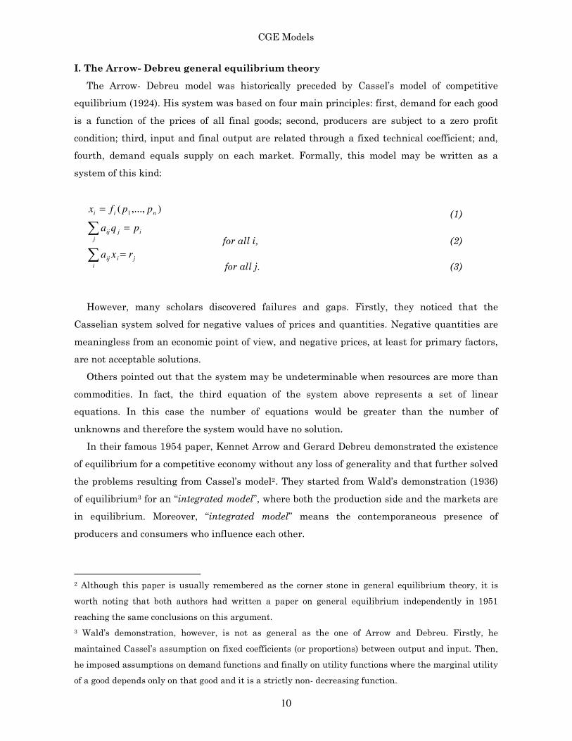
equilibrium (1924). His system was based on four main principles: first, demand for each good

is a function of the prices of all final goods; second, producers are subject to a zero profit

condition; third, input and final output are related through a fixed technical coefficient; and,

fourth, demand equals supply on each market. Formally, this model may be written as a

system of this kind:

),...,( 1 nii ppfx = (1)

∑ =j

ijij pqa

for all i, (2)

∑ =i

jiij rxa

for all j. (3)

However, many scholars discovered failures and gaps. Firstly, they noticed that the

Casselian system solved for negative values of prices and quantities. Negative quantities are

meaningless from an economic point of view, and negative prices, at least for primary factors,

are not acceptable solutions.

Others pointed out that the system may be undeterminable when resources are more than

commodities. In fact, the third equation of the system above represents a set of linear

equations. In this case the number of equations would be greater than the number of

unknowns and therefore the system would have no solution.

In their famous 1954 paper, Kennet Arrow and Gerard Debreu demonstrated the existence

of equilibrium for a competitive economy without any loss of generality and that further solved

the problems resulting from Cassel’s model2. They started from Wald’s demonstration (1936)

of equilibrium3 for an “integrated model”, where both the production side and the markets are

in equilibrium. Moreover, “integrated model” means the contemporaneous presence of

producers and consumers who influence each other.

2 Although this paper is usually remembered as the corner stone in general equilibrium theory, it is

worth noting that both authors had written a paper on general equilibrium independently in 1951

reaching the same conclusions on this argument.

3 Wald’s demonstration, however, is not as general as the one of Arrow and Debreu. Firstly, he

maintained Cassel’s assumption on fixed coefficients (or proportions) between output and input. Then,

he imposed assumptions on demand functions and finally on utility functions where the marginal utility

of a good depends only on that good and it is a strictly non- decreasing function.

CGE Models

11

Their starting point is a Walrasian economy of this fashion: “the solution of a system of

simultaneous equations representing the demand for goods by consumers, the supply of goods

by producers, and the equilibrium condition that supply equal demand on every market”

(Arrow, Debreu, 1954). Moreover, the fundamental assumptions are the same: “each consumer

acts so as to maximize his utility, each producer acts so as to maximize his profits, and perfect

competition prevails, in the sense that each producer and consumer regards the prices paid and

received as independent of his own choice” (Arrow, Debreu, 1954). Although Walras clearly had

defined the mechanism of this theoretical economy, he had not analyzed the assumptions on

equations in order to have a solution. As Arrow and Debreu stated “one check of the empirical

usefulness of the model is the prescription of the conditions under which the equations of

competitive equilibrium have a solution”. They derived two theorems that state very general

conditions for equilibrium. The first one asserts that if individuals have a certain positive

quantity of each commodity as its initial endowment, then equilibrium exists. The second

states that there should be two properties of labour: first, each individual should own at least

one type of labour (supposing there may be more than one labour type); second, this type of

labour should be employed for the production of commodities.

This reasoning allows for a generalized set of assumptions that are useful and applicable to

a wide variety of models (Arrow and Debreu, 1954; Duffie and Sonnenschein, 1989). Arrow

and Debreu’s work is structured as follows. First, their attention is devoted to the production

side, defining some basic concepts (i.e. commodity, production units) and the three

fundamental assumptions about production. Then, they move further to the consumption side

with the definition of consumption units, and a set of three other conditions on utility

functions. Finally, they present the market clearing conditions.

For a complete mathematical treatment, the reader is invited to see the original 1954

paper. Here we state the fundamental relationships and their implications.

In this competitive economy there is a finite number of commodities4, each one

characterized with respect to location and time, so that the same commodity sold or bought in

two places is treated as two distinct commodities and the same happens for a commodity sold

or bought today and tomorrow. We assume that L is the number of commodities and l, going

from 1 to L, designates different commodities. All vectors with l components are included in a

Euclidean space, RL, of l dimension.

4 The concept of commodity is a fundamental primitive concept in economic theory. Particularly, in

general equilibrium studies the concept of commodity is strictly linked to its nature. As Geanakoplos

(2004) underlies “general equilibrium theory is concerned with the allocation of commodities. […] The

Arrow-Debreu model studies those allocations which can be achieved trough the exchange of commodities

at one moment in time”.

CGE Models

12

Each of these vectors l is produced in a productive unit, or in other words a firm,

designated by the letter j. Each firm is characterized by its initial distribution of owners and a

specific technological production process. This means that there is a specific Yj for each firm

that represents the input - output combination5 for producing the commodity of firm j, and

there is a Y that is the summation of the different Yj over j. Therefore it represents all possible

input - output combinations seeing as the whole economy is a unique productive sector. So

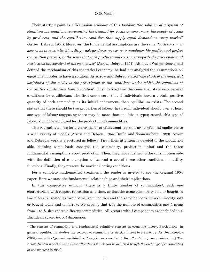
there are three assumptions about the nature of the set Yj.

First, increasing returns to scale, divisibility in production, and gains from specialization

are completely ruled out. Second, each aggregate production possibility vector, Y, must have at

least one negative component. This assumption is intuitive: each input is treated as a negative

entry (or component) so that this assumption simply states that each productive technology

requires at least one input. (There could not be any output without input). Finally, it is likely

to have a productive sector whose output is equal to the exact input for another production

process.

So, the starting point is the definition of the properties of the “technological aspects of

production,” which we may sum up mathematically:

1a) Yj is a convex subset of RL containing 0 (j= 1,…, n),

1b) 0=ΩΙY

1c) 0)( =−YY Ι

However, the technological aspects are not all that affect production. Productive decisions

also depend on the game rules. As usual, Arrow and Debreu assumed perfect competition so

that “the motivation for production is the maximization of profits taking prices as given”.

Formally speaking, this assumption leads to the first condition for general equilibrium:

I) y*

j maximizes jyp ⋅* over the set Yj, for each j.

Analogously, they assume the existence of another group of individuals called consumers

who are typically families or individuals. Let us denote with M the number of consumption

units, i defines the different consumption units that belong to the Euclidean space Ri. For any

marketed commodity, the rate of consumption is non negative6. Mathematically speaking:

5 Each component is composed of a positive entry which denotes output and a negative entry which is

input.

6 The only exception is labour. Supplied labour services are in fact counted as the negative of the rate of

consumption.

CGE Models

13

(2) the set of consumption vectors Xi available to individual i (= 1,…,M) is a closed convex

subset of Ri which is bounded from below; i.e. there is a vector ξi such that ii x≤ξ for all

iXix ∈ .

However, with this definition a new concept becomes relevant. The set Xi represents the

combination of all feasible consumption vectors7 where there is no budget constraint.

Moreover, it does not contain impossible combinations, such as the supply of more than 24

hours of labour (even of different types). According to Neoclassical theory, consumption choices

are assumed to be made according to a preference function called “utility indicator function”,

)( ixiu . As for the production possibility function, the utility function is characterized by three

assumptions about its properties.

First is the continuity requirement for function ui. This is a standard hypothesis in

consumers’ demand theory and follows the idea that consumption choices are made following

an order. Second, there is no consumption vector that is preferred over all others. This is

called the no saturation (or non-satiation) assumption. Finally, there is the usual assumption

on indifferent surfaces that are convex. However, convexity implies that commodities are

infinitely divisible and that any commodities’ combination is at least as good as the extreme.

Formally, these three conditions may be expressed this way:

3a) )( ixiu is a continuous function on Xi.

3b) For any ii Xx ∈ there is an ii Xx ∈' such that ).()( '

iiii xuxu >

3c) If )()( '

iiii xuxu > and 0 < t < 1, then )(])1([ ''

iiiii xuxttxu >−+ .

Moreover, a new condition must be assumed. As Arrow and Debreu pointed out, “to have

equilibrium it is necessary that each individual possess some asset or be capable of supplying

some labour service which commands a positive price at equilibrium”. Presuming that ζi is the

initial endowment of the ith consumption unit, composed of the initial available commodities,

following the 1954 paper we may define this condition as:

7 It is worth noting that when we speak of consumption we define consumption vectors that ultimately

are basket of commodities. In fact, consumption choices are made on the basis of a group of commodities

and not with respect to a single good. A single commodity has value only if compared to other

commodities that may be sold or bought. Together with the assumptions on transitivity and

completeness this representation of consumers’ preferences is precisely the neoclassical one.

CGE Models

14

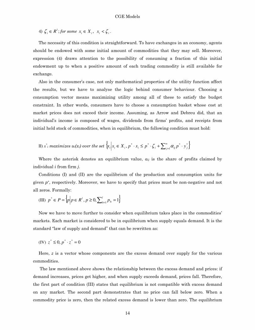
4) ;l

i R∈ζ for some ,ii Xx ∈ iix ζ< .

The necessity of this condition is straightforward. To have exchanges in an economy, agents

should be endowed with some initial amount of commodities that they may sell. Moreover,

expression (4) draws attention to the possibility of consuming a fraction of this initial

endowment up to when a positive amount of each trading commodity is still available for

exchange.

Also in the consumer’s case, not only mathematical properties of the utility function affect

the results, but we have to analyse the logic behind consumer behaviour. Choosing a

consumption vector means maximizing utility among all of these to satisfy the budget

constraint. In other words, consumers have to choose a consumption basket whose cost at

market prices does not exceed their income. Assuming, as Arrow and Debreu did, that an

individual’s income is composed of wages, dividends from firms’ profits, and receipts from

initial held stock of commodities, when in equilibrium, the following condition must hold:

II) x*i maximizes ui(xi) over the set ∑ =

⋅+⋅≤⋅∈n

j jijiiiii yppxpXxx1

****, αζ

Where the asterisk denotes an equilibrium value, αij is the share of profits claimed by

individual i from firm j.

Conditions (I) and (II) are the equilibrium of the production and consumption units for

given p*, respectively. Moreover, we have to specify that prices must be non-negative and not

all zeros. Formally:

(III) ∑ ==≥∈=∈

l

h h

lppRppPp

1

*1,0,

Now we have to move further to consider when equilibrium takes place in the commodities’

markets. Each market is considered to be in equilibrium when supply equals demand. It is the

standard “law of supply and demand” that can be rewritten as:

(IV) 0,0 *** =⋅≤ zpz

Here, z is a vector whose components are the excess demand over supply for the various

commodities.

The law mentioned above shows the relationship between the excess demand and prices: if

demand increases, prices get higher, and when supply exceeds demand, prices fall. Therefore,

the first part of condition (III) states that equilibrium is not compatible with excess demand

on any market. The second part demonstrates that no price can fall below zero. When a

commodity price is zero, then the related excess demand is lower than zero. The equilibrium

CGE Models

15

price vector *

p is a function of consumer demand and firms’ supply as well as of the primitive

data such as taste, technology and endowments (Duffie, Sonnenschein, 1989).

Now we have all the conditions and assumptions needed to define a general equilibrium.

First, the equilibrium is defined in terms of consumption quantities, produced output, and

final prices for different commodities. According to conditions (I) and (II), the maximizing

elements are quantities, production and consumption respectively, while condition (IV) refers

to prices. So Arrow and Debreu obtained a definition: “A set of vectors (***

1

** ,,...,,,..., pyyxx nmi) is

said to be a competitive equilibrium8 if it satisfies Conditions [(I)-(IV)]”.

In addition, this reasoning allows the authors to derive a theorem: “For any economic

system satisfying Assumptions [1-4] there is a competitive equilibrium”.

It may be helpful to stress some aspects of the Arrow-Debreu general equilibrium model

and some logical implications. Firstly, in this framework consumer and firm act independently

of each other within the same time period. This implies that both of these two groups act

according to their own rationale and they are motivated only by self- interest. At the same

time no agent acts before the other in the market, so that no one affects the price level by for

example setting prices. When the reasoning is expanded at the aggregate level, supply and

demand are equal and therefore determine the price level which guarantees equilibrium.

As Geanakoplos (2004) states, it is interesting to note that in the Arrow-Debreu model

there is a kind of “rational expectation”. This means that when agents act in the market, they

know every price to better allocate their choices. But, they also predict all future prices at the

end of the time period.

Although Arrow and Debreu’s model demonstrates the existence of a single equilibrium, it

also recognizes the possibility of multiple equilibria. The model, in fact, is adequate for

determining the value of the price vector on the basis of its primitives. As it is likely to

demonstrate, there are the possibilities of multiple equilibria in a Walrasian system. As Duffie

and Sonnenschein (1989) point out, “the equilibrium price set may be an essentially arbitrary

subset of the set of relative prices”. Therefore, it does not “tell us how to relate tastes,

technology, and the distribution of wealth to a single set of relative values. Rather, they tell us

8 The existence proof of the equilibrium employs the fixed-point theorem. To simply sum up the

reasoning, their demonstration follows three steps; first, they interpreted the economy as an abstract

economy or a generalised game, then they give the proof of the existence of at least one equilibrium of

this generalized game and finally they demonstrate that this equilibrium satisfies the clearing

condition on all markets.

CGE Models

16

that there is at least one vector (and possibly many more) of relative values compatible with the

data of the model”.

From a methodological point of view, this model innovation is a representation of a class of

assumptions that are necessary to have equilibrium, but at the same time are applicable to a

wide variety of models inside the marginalistic school. However to further extend the

applicability of the theorem, in 1971 Arrow and Hahn defined four presuppositions that must

be satisfied in order to reach an equilibrium.

These are the definition and construction of the excess-demand functions, their

homogeneity of degree zero, their continuity, and their satisfaction of Walras’s law. In this

way there is no reference to the marginalistic school, but only three technical hypotheses and

an accounting identity. Therefore, the applicability of this approach is extended to other

economic systems.

As Tucci (1997) points out, the approach is unique but it leads to a theory of multiple

equilibria. In this context, it means that the assumptions may be satisfied by many different

models. Each of them may be defined as general economic equilibrium characterized by a

specific economic context. The theorem appears as a minimum model so poor of economic

characteristics that may be easily applied in many contexts.

II. A standard representation of a CGE

The standard representation of a CGE model is nothing more than the transposition of the

Arrow-Debreu model in its simplest version. Therefore, the building of the model follows the

basic elements of the theoretical framework we have already discussed. In the simplest case

when the economy is closed and there is not any public sector, the applied model has only two

agents: firms and households (or consumers); both of them are considered to be price takers.

Then, each firm has a unique profit maximizing production plan, which affects commodities’

supply (and by aggregation the total supply). Each household’s income is a function of initial

endowments and their consumption is a function of income distribution and prices. Finally,

there is the usual excess-demand condition so that the difference between demand and supply

for each commodity is zero9.

9 More generally, Robinson (1989) defines that a CGE model must have four fundamental components.

“First, one must specify the economic actors or agents whose behaviour has to be analyzed. […] Second,

behavioural rules must be specified for these actors that reflect their assumed motivation. […] Third,

agents make their decisions based on signals they observe. […] Fourth, one must specify the rules of the

game according to which agents interact- the institutional structure of the economy”.

CGE Models

17

In the productive sphere, we suppose there are n firms, and each of them (called i) produces

a good j. This assumption is typical of input-output analysis. Then, there are two primary

factors: capital and labour. Gross sectoral output is a function of these factors according to a

certain degree of substitutability. So, formally the production function is often a CES

(Constant Elasticity of Substitution) function, which captures most of the interactions a

modeller wants to analyse. These two components create the value added component which is

embodied in the final product.

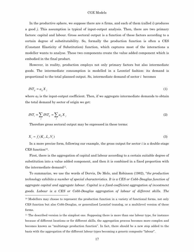
However, in reality, production employs not only primary factors but also intermediate

goods. The intermediate consumption is modelled in a Leontief fashion: its demand is

proportional to the total planned output. So, intermediate demand of sector i becomes

jijij XaINT = (1)

where aij is the input-output coefficient. Then, if we aggregate intermediate demands to obtain

the total demand by sector of origin we get:

∑∑ ==j

jij

j

iji XaINTINT (2)

Therefore gross sectoral output may be expressed in these terms:

),,( iiiii VLKfX = (3)

In a more precise form, following our example, the gross output for sector i is a double-stage

CES function10.

First, there is the aggregation of capital and labour according to a certain suitable degree of

substitution into a value added component, and then it is combined in a fixed proportion with

the intermediate demand11.

To summarize, we use the words of Dervis, De Melo, and Robinson (1982), “the production

technology exhibits a number of special characteristics. It is a CES or Cobb-Douglas function of

aggregate capital and aggregate labour. Capital is a fixed-coefficient aggregation of investment

goods. Labour is a CES or Cobb-Douglas aggregation of labour of different skills. The

10 Modellers may choose to represent the production function in a variety of functional forms, not only

CES function but also Cobb-Douglas, or generalised Leontief translog, or a multilevel version of these

forms.

11 The described version is the simplest one. Supposing there is more than one labour type, for instance

because of different locations or for different skills, the aggregation process becomes more complex and

becomes known as “multistage production function”. In fact, there should be a new step added to the

basis with the aggregation of the different labour types becoming a generic composite “labour”.

CGE Models

18

production function is thus a two-level function. Intermediate goods are required according to

fixed coefficients and so can be treated separately”.

With respect to the Arrow-Debreu conditions on production, it is instinctive to understand

that this modelling satisfies the assumptions 1a, 1b, and 1c presented in the previous

paragraph. In fact, the CES function (or the Cobb-Douglas as a particular case) presents

decreasing returns to scale, so that the first assumption is satisfied. Then, the construction of

the production function implies that there is at least one input to produce a certain amount of

output and whenever input is zero, production is also zero. Finally, it is likely that a

productive sector’s output is completely devoted to intermediate consumption.

With the production function, the modeller describes the technological conditions under

which production takes place. But other assumptions should be made on factors of production,

in particular on their mobility among sectors. Capital is usually assumed to be fixed at the

beginning of each period. This seems quite reasonable: an increase in capital is due to an

increase in investments which can take place only at the end of the time period, so that a

higher capital stock is available only in the next time period. However, labour is mobile across

sectors.

The production set is incomplete if we do not define a set of factor availability constraints.

They may be written as demand excess functions for the productive factors. For instance,

labour constraint may be written as:

∑ =−i

iis LL 0 (4)

Here, sectoral labour supply Li is fixed and equals the sum of different labour skill

categories employed in the i sector.

Until now we have described the “production possibility set” that is the “technical

description of attainable combinations of output” (Dervis, de Melo, Robinson 1982). But to

complete the supply side we have to consider the market behaviour too. In this way we derive

the “transformation set”.

According to the marginalistic paradigm, producers are supposed to be maximizing agents.

Their objective is to maximize their profits assuming that the market acts in perfect

competition so that firms take prices as they are given. As previously emphasized, in this

simplified example there is no Government. Therefore, the profit equation may be written as:

∑−=Πi

isiii LwPN (5)

Here, PNi is the net price, or in other words, the output price minus the intermediate

component. From the Shepard’s lemma, we know that wages equal the value of marginal

CGE Models

19

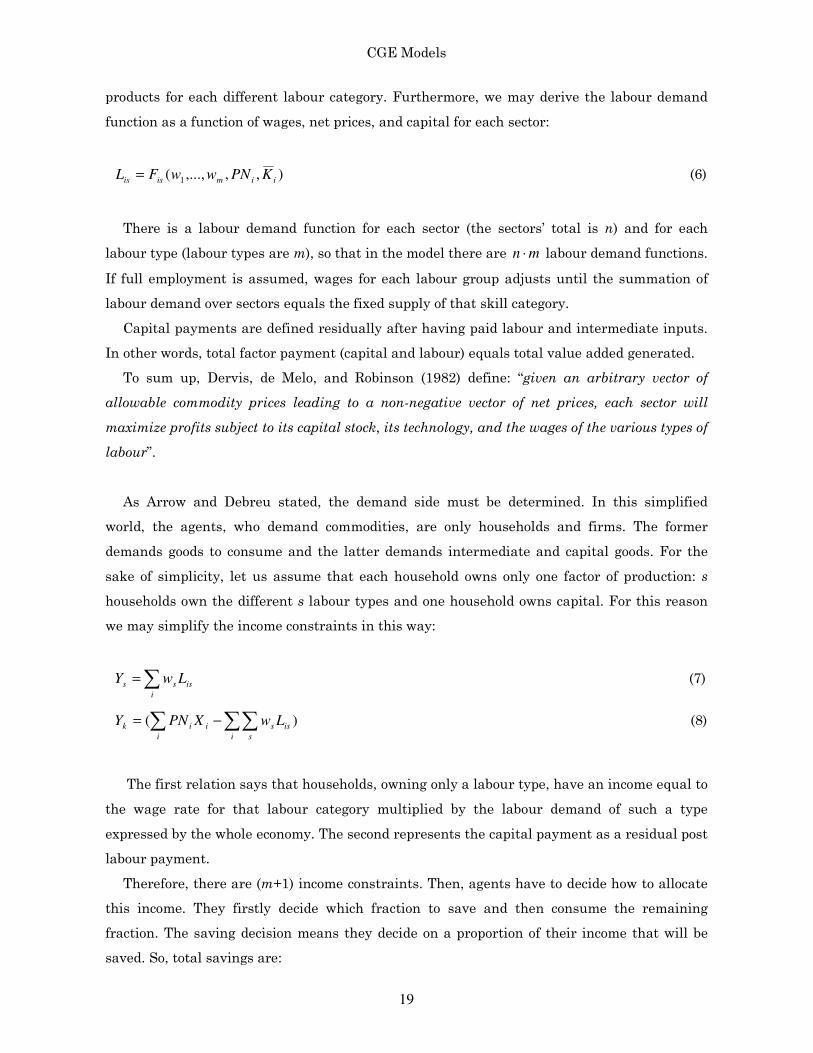
products for each different labour category. Furthermore, we may derive the labour demand

function as a function of wages, net prices, and capital for each sector:

),,,...,( 1 iimisis KPNwwFL = (6)

There is a labour demand function for each sector (the sectors’ total is n) and for each

labour type (labour types are m), so that in the model there are mn ⋅ labour demand functions.

If full employment is assumed, wages for each labour group adjusts until the summation of

labour demand over sectors equals the fixed supply of that skill category.

Capital payments are defined residually after having paid labour and intermediate inputs.

In other words, total factor payment (capital and labour) equals total value added generated.

To sum up, Dervis, de Melo, and Robinson (1982) define: “given an arbitrary vector of

allowable commodity prices leading to a non-negative vector of net prices, each sector will

maximize profits subject to its capital stock, its technology, and the wages of the various types of

labour”.

As Arrow and Debreu stated, the demand side must be determined. In this simplified

world, the agents, who demand commodities, are only households and firms. The former

demands goods to consume and the latter demands intermediate and capital goods. For the

sake of simplicity, let us assume that each household owns only one factor of production: s

households own the different s labour types and one household owns capital. For this reason

we may simplify the income constraints in this way:

∑=i

isss LwY (7)

)(∑ ∑∑−=i i s

issiik LwXPNY (8)

The first relation says that households, owning only a labour type, have an income equal to

the wage rate for that labour category multiplied by the labour demand of such a type

expressed by the whole economy. The second represents the capital payment as a residual post

labour payment.

Therefore, there are (m+1) income constraints. Then, agents have to decide how to allocate

this income. They firstly decide which fraction to save and then consume the remaining

fraction. The saving decision means they decide on a proportion of their income that will be

saved. So, total savings are:

CGE Models

20

kk

s

ss YsYsTS +=∑ (9)

So, we formalize the consumption functions12 as functions of price level for the different

commodities, and the available income after saving decisions. Therefore we have:

])1(,,...,[ 1 ssnis

D

is YsPPCC −= (10)

])1(,,...,[ 1 kknik

D

ik YsPPCC −= (11)

Then, aggregating the demand functions we have the total demand:

])1(,,...,[])1(,,...,[ 211 kkikssn

s

D

is

D

i YsPPCYsPPCC −+−=∑ (12)

At first glance we may say that consumption depends upon commodities’ prices and

personal income (or in other words the factors’ payments). But, although this idea is correct,

we may simply state that demand functions depend only on the price level. Recalling the

definition of Dervis et al., the first step in CGE is to give a final price factor. Once given, the

factor payment is the consequence. So the consumption vector function may be simplified as:

),...,( 1 n

DPPCC = (13)

To quote Dervis, de Melo and Robinson (1982): “it is understood that behind the equation

lies the solution of factor market as well as the various equations defining disposable income.

Fundamentally, however, there is a simple chain of causality leading from the price vector to

the vector of consumption demand”.

From the discussion about consumption we have derived a new aggregate, total savings. It

is usually assumed to be completely devoted to investments. It is likely to write the

investment demand function as a function of the initial price vector:

),...,( 1 ni PPZZ = (14)

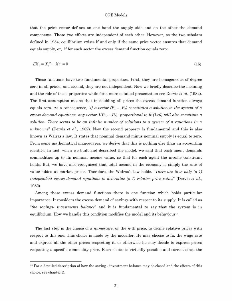
Finally, the third condition in the Arrow-Debreu model regards market equilibrium or in

other words the excess demand equations for commodities. Up to this point we have concluded

12 Functionally, there are many different consumption functions. The simplest one is the Cobb-Douglas

function. Probably the most used is the linear expenditure system.

CGE Models

21

that the price vector defines on one hand the supply side and on the other the demand

components. These two effects are independent of each other. However, as the two scholars

defined in 1954, equilibrium exists if and only if the same price vector ensures that demand

equals supply, or, if for each sector the excess demand function equals zero:

0=−= S

i

D

ii XXEX (15)

These functions have two fundamental properties. First, they are homogeneous of degree

zero in all prices, and second, they are not independent. Now we briefly describe the meaning

and the role of these properties while for a more detailed presentation see Dervis et al. (1982).

The first assumption means that in doubling all prices the excess demand function always

equals zero. As a consequence, “if a vector (P1,…,Pn) constitutes a solution to the system of n

excess demand equations, any vector λ(P1,…,Pn) proportional to it (λ>0) will also constitute a

solution. There seems to be an infinite number of solutions to a system of n equations in n

unknowns” (Dervis et al., 1982). Now the second property is fundamental and this is also

known as Walras’s law. It states that nominal demand minus nominal supply is equal to zero.

From some mathematical manoeuvres, we derive that this is nothing else than an accounting

identity. In fact, when we built and described the model, we said that each agent demands

commodities up to its nominal income value, so that for each agent the income constraint

holds. But, we have also recognized that total income in the economy is simply the rate of

value added at market prices. Therefore, the Walras’s law holds. “There are thus only (n-1)

independent excess demand equations to determine (n-1) relative price ratios” (Dervis et al.,

1982).

Among these excess demand functions there is one function which holds particular

importance. It considers the excess demand of savings with respect to its supply. It is called as

“the savings- investments balance” and it is fundamental to say that the system is in

equilibrium. How we handle this condition modifies the model and its behaviour13.

The last step is the choice of a numeraire, or the n-th price, to define relative prices with

respect to this one. This choice is made by the modeller. He may choose to fix the wage rate

and express all the other prices respecting it, or otherwise he may decide to express prices

respecting a specific commodity price. Each choice is virtually possible and correct since the

13 For a detailed description of how the saving - investment balance may be closed and the effects of this

choice, see chapter 2.

CGE Models

22

theory does not impose any restrictions on the numeraire. Some modellers, however, prefer “a

non-inflation benchmark”. They create a weighted average of the prices in the economy using

an index that may be remain stable, or may be changed over time in order to reflect projected

changes in some price indexes.

Until now we have considered the simple case when, in the economy only s households and i

productive sectors exist. We may easily extend the model to introduce a new agent, the

Government, and analyze how it affects these relationships. Firstly, like any agent, the

Government has an income. It draws not only from factors’ property but also from tax

payments. It may impose many different taxes; for instance a taxation on household nominal

income, or a tax on factor uses, or indirect taxes on commodities’ consumption. To simplify our

analysis we assume only a tax on household income.

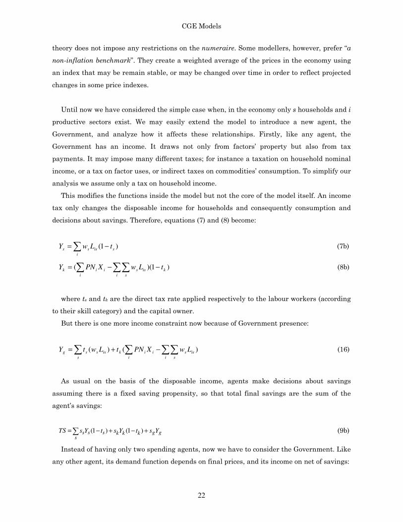
This modifies the functions inside the model but not the core of the model itself. An income

tax only changes the disposable income for households and consequently consumption and

decisions about savings. Therefore, equations (7) and (8) become:

∑ −=i

sisss tLwY )1( (7b)

∑ ∑∑ −−=i i

k

s

issiik tLwXPNY )1)(( (8b)

where ts and tk are the direct tax rate applied respectively to the labour workers (according

to their skill category) and the capital owner.

But there is one more income constraint now because of Government presence:

∑∑∑∑ −+=i s

iss

i

iik

s

isssg LwXPNtLwtY )()( (16)

As usual on the basis of the disposable income, agents make decisions about savings

assuming there is a fixed saving propensity, so that total final savings are the sum of the

agent’s savings:

(1 ) (1 )s s s g gk k ks

TS s Y t s Y t s Y= − + − +∑ (9b)

Instead of having only two spending agents, now we have to consider the Government. Like

any other agent, its demand function depends on final prices, and its income on net of savings:

CGE Models

23

])1(,,...,[ 1 ggnig

D

ig YsPPCC −= (17)

Finally, the aggregate demand function has not two but three addends because we have to

consider demand for the different household categories and for the Government.

In this chapter we limit the exposition of standard CGE models to the case of a closed

economy with Government. However, this tool may also be applied and used for open economy

issues. These kinds of models will be analyzed in details in the following chapter where we

present many different ways of interpreting and modelling the foreign sector.

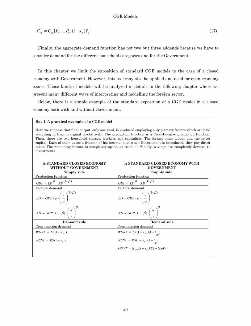
Below, there is a simple example of the standard exposition of a CGE model in a closed

economy both with and without Government.

Box 1: A practical example of a CGE model

Here we suppose that final output, only one good, is produced employing only primary factors which are paid

according to their marginal productivity. The production function is a Cobb-Douglas production function.

Then, there are two household classes, workers and capitalists. The former owns labour and the latter

capital. Each of them saves a fraction of his income, and, when Government is introduced, they pay direct

taxes. The remaining income is completely spent, as residual. Finally, savings are completely devoted to

investments.

A STANDARD CLOSED ECONOMY

WITHOUT GOVERNMENT

A STANDARD CLOSED ECONOMY WITH

GOVERNMENT

Supply side Supply side

Production function Production function

)1( ββ −⋅= KDLDGDP

)1( ββ −⋅= KDLDGDP

Factors’ demand Factors’ demand

)1( β

β

−

⋅⋅=

w

rGDPLD

)1( β

β

−

⋅⋅=

w

rGDPLD

β

β

⋅−⋅=

r

wGDPKD )1(

β

β

⋅−⋅=

r

wGDPKD )1(

Demand side Demand side

Consumption demand Consumption demand

)1( wsLSWORK −= )1)(1(w

twsLSWORK −−=

)1( rsKSRENT −= )1)(1(r

trsKSRENT −−=

GSAVKSrtLSwtGOVT −+= )(

CGE Models

24

(Box 1 continues)

Excess demand constraints Excess demand constraints

INVPXRENTWORKGDP ++= /)( INVPXGOVTRENTWORKGDP +++= /)( LSLD = LSLD = KSKD = KSKD =

0)( =⋅−+ INVPXKSrsLSws

0)( =⋅−++ INVPXGSAVKSrsLSws

GDP= nominal production, LD= labour demand, KD= capital demand, LS= labour supply, KS= capital

supply, r= rental rate of capital, w=wage rate, WORK= nominal workers’ consumption, RENT= nominal

capitalists’ consumption, sw= saving propensity for workers, sr= saving propensity for capitalists, INV=

real investments, PX= output price, GOVT= nominal government consumption, tw= direct tax rate on

workers, tr= direct tax rate on capitalists, GSAV= nominal government saving.

III. Partial vs General Equilibrium

The effects of an economic shock are usually studied and evaluated using two different

methods: partial equilibrium analysis and general equilibrium analysis. As already described,

general equilibrium analysis exploits inter-market relationships in order to analyze economy-

wide effects on the whole economic structure. Partial equilibrium analysis, following the

tradition of Alfred Marshall, focuses on a single market so that it can explore the effects on

one market and no second round effects on other markets. It is usually referred to as the

“ceteris paribus” assumption, where all relevant variables, except the price in question, are

constant. In this case, prices of substitutes, complements, and consumers’ income are assumed

to be constant.

This tool is useful when the goal is to analyse a single commodity market whose size is

small compared to the economy as a whole.

This approach is mainly based on the demand - supply analysis, assuming the existence of

a supply curve and a demand curve, which respectively represent the marginal social cost

curve and the marginal social benefit curve. Let us explore the effects of a reduction in

production costs for a specific sector. Let’s suppose that starting in a position of equilibrium, a

cost reduction means an increase in supply because of the lower unitary cost.

Therefore, if the firm wants to spend the same amount of money, it should produce a higher

level of output. But, higher supply lowers final prices. When prices go down, consumers have

an incentive to buy more. In this way, at a new price level, the economy reaches equilibrium.

Typically, partial equilibrium analyses are applied in welfare analysis when a single

market is involved. This is the case, for example, of a change in import duties for a specific

good, or the imposition of a sales tax for a good.

CGE Models

25

Figure 1: A diagrammatical representation

A

B

C

D

E

F

Supply

Demand

q* qd

Pd

P*

Ps

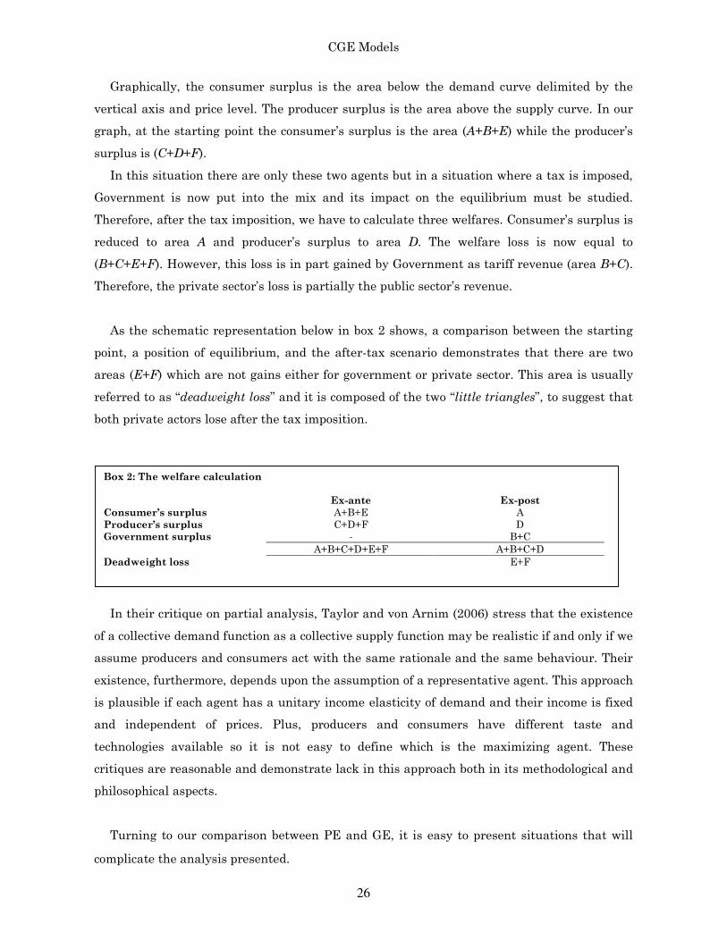
To better define the differences and which elements are captured by the two approaches, we

concentrate on the case of a new import tax on a specific good. Let us suppose this good is

called A, which is both produced domestically and imported. This analysis is based on the

usual downward sloping demand curve and the upward sloping supply curve in the space

(P,q). The diagrammatical description is provided in graph 1 according to the contemporary

version of the theory. As it is defined, the demand curve represents the willingness of

customers to pay, in other words each combination (P, q) represents the price P consumers are

willing to pay for the quantity q. The supply curve represents, given the price, the total

amount of output firms want in order to supply in the market. In this case these curves

represent the demand and supply at the national level for good A. At the starting point price

equals P* and the quantity is q*. However, the introduction of the tariff, with a rate tm,

increases the prices up to the level P(1+tm), here defined as Pd. As a consequence, demand has

been reduced to level qd. Because of the higher price, consumers reduce their consumption and

at the same time producers reduce their surplus. In fact, at the quantity level qd, they obtain

only Ps as price. The wedge between Ps and Pd represents the exact tax rate imposed by the

Government.

The economy reaches a new equilibrium position with a lower marketed quantity and a

higher price. Usually this framework is employed to answer questions like: who gains from the

imposition of an import tax? How much is the loss of consumers?

To answer these, and similar questions, we have to analyse what is commonly defined as

the “little triangles” (von Arnim, Taylor, 2006). The fundamental concepts are the consumer

and the producer surpluses. The former consists of the benefit accumulated by consumers in

the market from buying the good, while the latter is the benefit accumulated by producers

selling the same good. To solve the welfare calculations we refer to the graph below.

Source: Taylor, von Arnim (2006)

CGE Models

26

Graphically, the consumer surplus is the area below the demand curve delimited by the

vertical axis and price level. The producer surplus is the area above the supply curve. In our

graph, at the starting point the consumer’s surplus is the area (A+B+E) while the producer’s

surplus is (C+D+F).

In this situation there are only these two agents but in a situation where a tax is imposed,

Government is now put into the mix and its impact on the equilibrium must be studied.

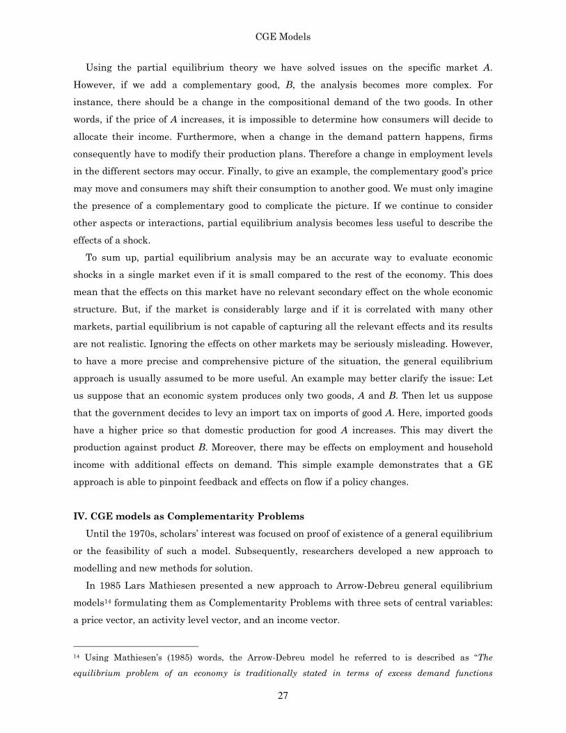
Therefore, after the tax imposition, we have to calculate three welfares. Consumer’s surplus is

reduced to area A and producer’s surplus to area D. The welfare loss is now equal to

(B+C+E+F). However, this loss is in part gained by Government as tariff revenue (area B+C).

Therefore, the private sector’s loss is partially the public sector’s revenue.

As the schematic representation below in box 2 shows, a comparison between the starting

point, a position of equilibrium, and the after-tax scenario demonstrates that there are two

areas (E+F) which are not gains either for government or private sector. This area is usually

referred to as “deadweight loss” and it is composed of the two “little triangles”, to suggest that

both private actors lose after the tax imposition.

In their critique on partial analysis, Taylor and von Arnim (2006) stress that the existence

of a collective demand function as a collective supply function may be realistic if and only if we

assume producers and consumers act with the same rationale and the same behaviour. Their

existence, furthermore, depends upon the assumption of a representative agent. This approach

is plausible if each agent has a unitary income elasticity of demand and their income is fixed

and independent of prices. Plus, producers and consumers have different taste and

technologies available so it is not easy to define which is the maximizing agent. These

critiques are reasonable and demonstrate lack in this approach both in its methodological and

philosophical aspects.

Turning to our comparison between PE and GE, it is easy to present situations that will

complicate the analysis presented.

Box 2: The welfare calculation Ex-ante Ex-post

Consumer’s surplus A+B+E A

Producer’s surplus C+D+F D

Government surplus - B+C

A+B+C+D+E+F A+B+C+D

Deadweight loss E+F

CGE Models

27

Using the partial equilibrium theory we have solved issues on the specific market A.

However, if we add a complementary good, B, the analysis becomes more complex. For

instance, there should be a change in the compositional demand of the two goods. In other

words, if the price of A increases, it is impossible to determine how consumers will decide to

allocate their income. Furthermore, when a change in the demand pattern happens, firms

consequently have to modify their production plans. Therefore a change in employment levels

in the different sectors may occur. Finally, to give an example, the complementary good’s price

may move and consumers may shift their consumption to another good. We must only imagine

the presence of a complementary good to complicate the picture. If we continue to consider

other aspects or interactions, partial equilibrium analysis becomes less useful to describe the

effects of a shock.

To sum up, partial equilibrium analysis may be an accurate way to evaluate economic

shocks in a single market even if it is small compared to the rest of the economy. This does

mean that the effects on this market have no relevant secondary effect on the whole economic

structure. But, if the market is considerably large and if it is correlated with many other

markets, partial equilibrium is not capable of capturing all the relevant effects and its results

are not realistic. Ignoring the effects on other markets may be seriously misleading. However,

to have a more precise and comprehensive picture of the situation, the general equilibrium

approach is usually assumed to be more useful. An example may better clarify the issue: Let

us suppose that an economic system produces only two goods, A and B. Then let us suppose

that the government decides to levy an import tax on imports of good A. Here, imported goods

have a higher price so that domestic production for good A increases. This may divert the

production against product B. Moreover, there may be effects on employment and household

income with additional effects on demand. This simple example demonstrates that a GE

approach is able to pinpoint feedback and effects on flow if a policy changes.

IV. CGE models as Complementarity Problems

Until the 1970s, scholars’ interest was focused on proof of existence of a general equilibrium

or the feasibility of such a model. Subsequently, researchers developed a new approach to

modelling and new methods for solution.

In 1985 Lars Mathiesen presented a new approach to Arrow-Debreu general equilibrium

models14 formulating them as Complementarity Problems with three sets of central variables:

a price vector, an activity level vector, and an income vector.

14 Using Mathiesen’s (1985) words, the Arrow-Debreu model he referred to is described as “The

equilibrium problem of an economy is traditionally stated in terms of excess demand functions

CGE Models

28

As he demonstrated, equilibrium among these three variables satisfies a system of three

classes of nonlinear inequalities commonly defined as zero profit conditions, market clearance

conditions, and income balance conditions. However, these three conditions have already been

recognized as fundamental elements for defining general equilibrium since Arrow-Debreu

works (paragraph II).

Here, we present each of these groups, analysing how the final relations are derived from a

mathematical point of view, and the economic meaning of each relation.

Let us suppose that in this economic system there are n commodities, m productive units,

and p consumers. Each of them is indexed respectively by i, j, and k.

There are many ways in which scholars demonstrate how to derive equilibrium conditions.

Here we apply the one in Dixit- Norman (1980). As they affirm: “as the ultimate objective of

equilibrium theory is to examine how the actions of different price taking agents fit together, the

natural building blocks should use prices as independent variables. This is best done using

duality i.e. modelling consumer behaviour by means of expenditure or indirect utility functions,

and producer behaviour by means of cost, revenue or profit functions”.

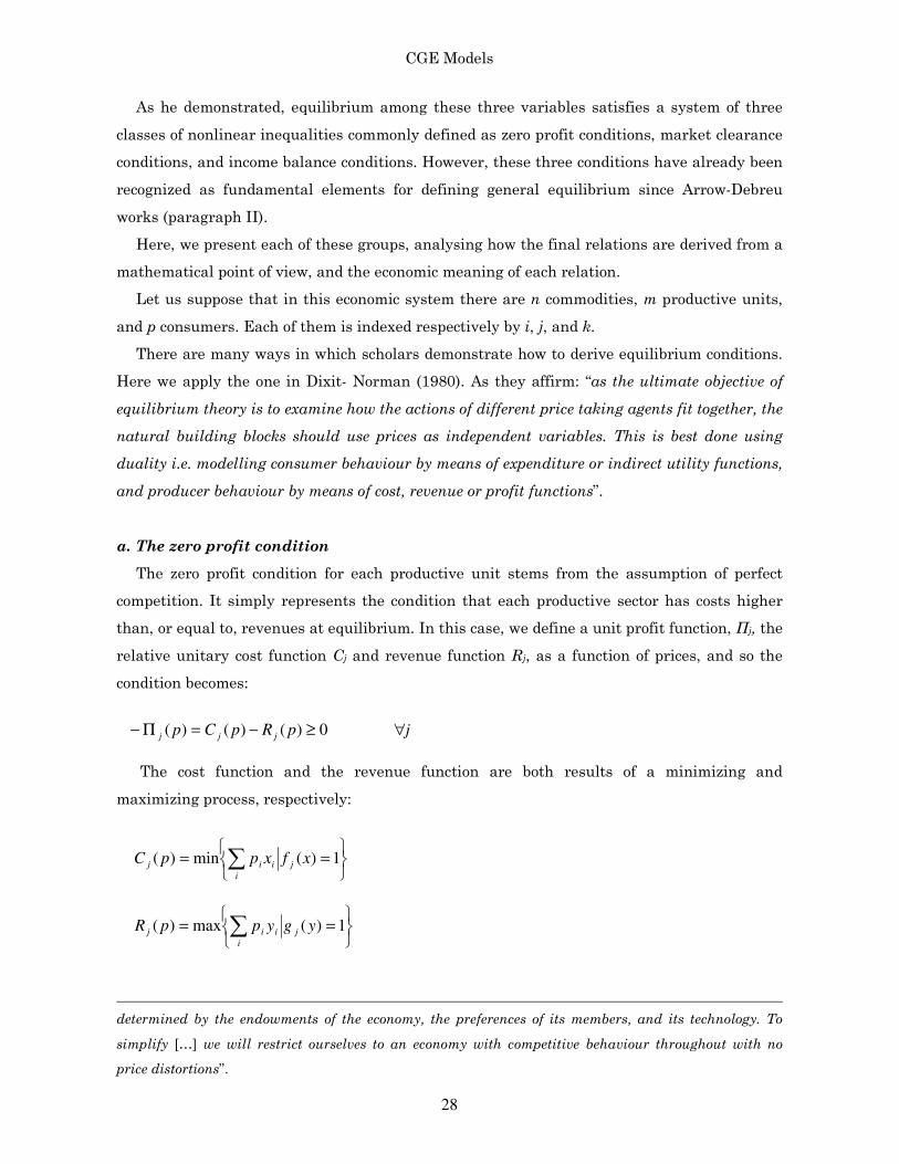
a. The zero profit condition

The zero profit condition for each productive unit stems from the assumption of perfect

competition. It simply represents the condition that each productive sector has costs higher

than, or equal to, revenues at equilibrium. In this case, we define a unit profit function, Πj, the

relative unitary cost function Cj and revenue function Rj, as a function of prices, and so the

condition becomes:

0)()()( ≥−=Π− pRpCp jjj j∀

The cost function and the revenue function are both results of a minimizing and

maximizing process, respectively:

== ∑i

jiij xfxppC 1)(min)(

== ∑i

jiij ygyppR 1)(max)(

determined by the endowments of the economy, the preferences of its members, and its technology. To

simplify […] we will restrict ourselves to an economy with competitive behaviour throughout with no

price distortions”.

CGE Models

29

Where f(x) is the aggregating function for input, and g(y) is the aggregating function for

final production.

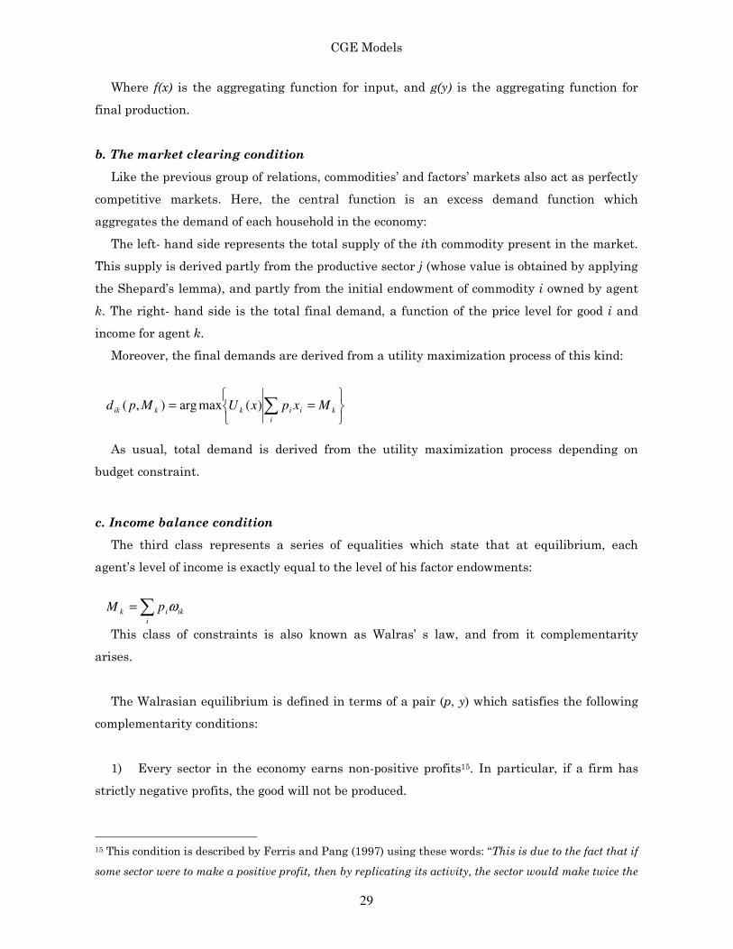
b. The market clearing condition

Like the previous group of relations, commodities’ and factors’ markets also act as perfectly

competitive markets. Here, the central function is an excess demand function which

aggregates the demand of each household in the economy:

The left- hand side represents the total supply of the ith commodity present in the market.

This supply is derived partly from the productive sector j (whose value is obtained by applying

the Shepard’s lemma), and partly from the initial endowment of commodity i owned by agent

k. The right- hand side is the total final demand, a function of the price level for good i and

income for agent k.

Moreover, the final demands are derived from a utility maximization process of this kind:

== ∑i

kiikkik MxpxUMpd )(maxarg),(

As usual, total demand is derived from the utility maximization process depending on

budget constraint.

c. Income balance condition

The third class represents a series of equalities which state that at equilibrium, each

agent’s level of income is exactly equal to the level of his factor endowments:

∑=i

ikik pM ω

This class of constraints is also known as Walras’ s law, and from it complementarity

arises.

The Walrasian equilibrium is defined in terms of a pair (p, y) which satisfies the following

complementarity conditions:

1) Every sector in the economy earns non-positive profits15. In particular, if a firm has

strictly negative profits, the good will not be produced.

15 This condition is described by Ferris and Pang (1997) using these words: “This is due to the fact that if

some sector were to make a positive profit, then by replicating its activity, the sector would make twice the

CGE Models

30

2) Supply minus demand for each good is non-negative. However, if supply exceeds demand

then the relative price will be zero.

There are other observations to be made. First, supposing that the utility function that we

derive the demand function from exhibits non-satiation, according to Walras’s law

expenditures exhaust agents’ budgets:

∑ ∑==i i

ikikiki pMdp ω

Combining the conditions above and if the excess demand function satisfies Walras’ s law,

then complementary slackness conditions are automatically satisfied. Moreover, they are a

feature of equilibrium itself and not a condition for it.

Formally:

0),()(

=

−+

∂

Π∂∑ ∑∑

j k

kik

k

ik

i

j

ji Mpdp

pyp ω i∀

Next, the demand function is homogenous of degree zero so that if the pair (p, y) is an

equilibrium, then the pairs (λp, y), for all λ > 0, are other equilibria. Therefore “relative rather

than absolute prices determine an equilibrium” (Rutherford, 1987).

profit, and thus its total profit would be unbound. Intuitively, the mimicking behaviour drives the price

of the corresponding commodity down and hence reduces the profitability of that commodity”.

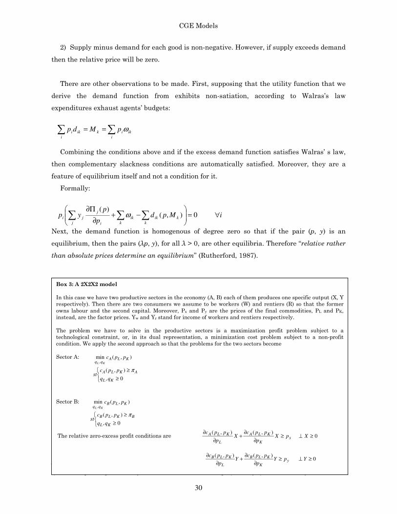
Box 3: A 2X2X2 model

In this case we have two productive sectors in the economy (A, B) each of them produces one specific output (X, Y

respectively). Then there are two consumers we assume to be workers (W) and rentiers (R) so that the former

owns labour and the second capital. Moreover, Px and Py are the prices of the final commodities, PL and PK,

instead, are the factor prices. Yw and Yr stand for income of workers and rentiers respectively.

The problem we have to solve in the productive sectors is a maximization profit problem subject to a

technological constraint, or, in its dual representation, a minimization cost problem subject to a non-profit

condition. We apply the second approach so that the problems for the two sectors become

Sector A: ),(min,

KLAqq

ppcKL

≥

≥

0,

),(

KL

AKLA

qq

ppcst

π

Sector B: ),(min,

KLBqq

ppcKL

≥

≥

0,

),(

KL

BKLB

qq

ppcst

π

The relative zero-excess profit conditions are xK

KLA

L

KLA pXp

ppcX

p

ppc≥

∂

∂+

∂

∂ ),(),( 0≥⊥ X

yK

KLB

L

KLB pYp

ppcY

p

ppc≥

∂

∂+

∂

∂ ),(),( 0≥⊥ Y

CGE Models

31

(Box 3 continues)

When we consider the two consumers we have to solve a maximization problem as well. They want to maximize

the utility they derive from consumption subject to a budget constraint that is represented by their income. Or,

as in the case above, the problem may be interpreted in its dual formulation. The problem becomes a minimizing

cost problem given a certain level of utility they want to obtain:

Consumer W: ),(max,

yxWqq

qquyx

≥

≤

0,

),(

yx

WyxW

pp

Mppest

Consumer R ),(max,

yxRqq

qquyx

≥

≤

0,

),(

yx

RyxR

pp

Mppest

When solving these problems we obtain four demands: a pair for each consumer:

Demand for consumer W of good X: ),(, WxWx Ypξ

Demand for consumer W of good Y: ),(, WyWy Ypξ

Demand for consumer R of good X: ),(, RxRx Ypξ

Demand for consumer R of good Y: ),(, RyRy Ypξ

These demands enter the market clearance conditions for each commodity market:

≥X +),(, WxWx Ypξ ),(, RxRx Ypξ

≥Y +),(, WyWy Ypξ ),(, RyRy Ypξ

But there are another two markets, the factors markets, where supply and demand exist:

Yp

ppcX

p

ppcL

L

KLB

L

KLA

∂

∂+

∂

∂≥

),(),(

≥K +∂

∂X

p

ppc

K

KLA ),(Y

p

ppc

K

KLB

∂

∂ ),(

Therefore, the market clearing conditions and the related slackness conditions are:

≥X +),(, WxWx Ypξ ),(, RxRx Ypξ 0≥⊥ xp

≥Y +),(, WyWy Ypξ ),(, RyRy Ypξ 0≥⊥ yp

Yppc

Xppc

L KLBKLA ∂+

∂≥

),(),( 0≥⊥ p

To sum up, the GE equilibrium conditions have become a NLCP (Non Linear

Complementarity Problem), whose general formal representation is the following:

Given : N NF ℜ → ℜ

Find , 0Nz z∈ℜ ≥ such that ( ) 0F z ≥ ' ( ) 0z F z =

This formal statement is nothing other than the definition of the Karush- Khun- Thucker

(KKT) conditions for the solution of max/min problems with inequality constraints. This

specification is useful when we want to detect how empirically we may derive the GE

conditions. This is the goal of box 3 below. We focus on the productive sector and we derive its

CGE Models

32

equilibrium condition. We exploit the KKT conditions to demonstrate that what we obtain is

exactly the zero profit condition we have previously presented in its general format.

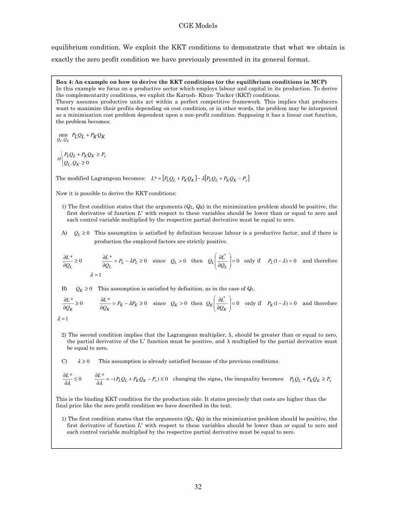
Box 4: An example on how to derive the KKT conditions (or the equilibrium conditions in MCP)

In this example we focus on a productive sector which employs labour and capital in its production. To derive

the complementarity conditions, we exploit the Karush- Khun- Tucker (KKT) conditions.

Theory assumes productive units act within a perfect competitive framework. This implies that producers

want to maximize their profits depending on cost condition, or in other words, the problem may be interpreted

as a minimization cost problem dependent upon a non-profit condition. Supposing it has a linear cost function,

the problem becomes:

KL QQ ,min KQKPLQLP +

≥

≥+

0, KL

xKKLL

QQ

PQPQPst

The modified Lagrangean becomes: [ ] [ ]xKKLLKKLL PQPQPQPQPL −+−+= λ*

Now it is possible to derive the KKT conditions:

1) The first condition states that the arguments (QL, QK) in the minimization problem should be positive, the

first derivative of function L* with respect to these variables should be lower than or equal to zero and

each control variable multiplied by the respective partial derivative must be equal to zero.

A) 0≥LQ This assumption is satisfied by definition because labour is a productive factor, and if there is

production the employed factors are strictly positive.

0*

≥∂

∂

LQ

L 0

*≥−=

∂

∂LL

L

PPQ

Lλ since 0>LQ then 0

*

=

∂

∂

LL

Q

LQ only if 0)1( =− λLP and therefore

1=λ

B) 0≥KQ This assumption is satisfied by definition, as in the case of QL.

0*

≥∂

∂

KQ

L 0

*≥−=

∂

∂KK

K

PPQ

Lλ since 0>KQ then 0

*

=

∂

∂

KK

Q

LQ only if 0)1( =− λKP and therefore

1=λ

2) The second condition implies that the Lagrangean multiplier, λ, should be greater than or equal to zero,

the partial derivative of the L* function must be positive, and λ multiplied by the partial derivative must

be equal to zero.

C) 0≥λ This assumption is already satisfied because of the previous conditions.

0*

≤∂

∂

λ

L 0)(

*≤−+−=

∂

∂xKKLL PQPQP

L

λ changing the signs, the inequality becomes: xKKLL PQPQP ≥+

This is the binding KKT condition for the production side. It states precisely that costs are higher than the

final price like the zero profit condition we have described in the text.

1) The first condition states that the arguments (QL, QK) in the minimization problem should be positive, the

first derivative of function L* with respect to these variables should be lower than or equal to zero and

each control variable multiplied by the respective partial derivative must be equal to zero.

CGE Models

33

Although originally applied for Walrasian equilibria, this interpretation may be modified in

order to be applied in different contexts, for instance when a public sector exists. In this case,

taxes modify the relationships between prices and the allocation of income. For example, tax

imposed on factors modifies their employment because they become more expensive and their

prices are unable to move independently to clear their markets. Instead, if an income tax is

imposed, income will not be equal to total expenditures because households have to pay a

certain amount to the Government. As Ferris and Pang (1997) point out “when taxes are

applied to inputs or outputs, the profitability of the corresponding sectors and how the sectors

technology is operated may be affected”.

Let us consider a tax on inputs and a tax on final production, whose tax rates are tl, tk and

tx, respectively. Let us suppose this makes the producer’s problem change. He already wants

to maximize his profits but this time the revenue function and the cost function are altered by

the presence of these two taxes. Namely, inputs have higher costs now because their prices

become (1+tl)Pl and (1+tk)Pk, instead of Pl and Pk.

The opposite happens for final products: their prices are lowered because a certain rate

accrues to the Government so that producers’ revenues are lowered.

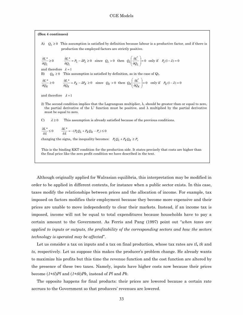
(Box 4 continues)

A) 0≥LQ This assumption is satisfied by definition because labour is a productive factor, and if there is

production the employed factors are strictly positive.

0*

≥∂

∂

LQ

L 0

*≥−=

∂

∂LL

L

PPQ

Lλ since 0>LQ then 0

*

=

∂

∂

LL

Q

LQ only if 0)1( =− λLP

and therefore 1=λ

B) 0≥KQ This assumption is satisfied by definition, as in the case of QL.

0*

≥∂

∂

KQ

L 0

*≥−=

∂

∂KK

K

PPQ

Lλ since 0>KQ then 0

*

=

∂

∂

KK

Q

LQ only if 0)1( =− λKP

and therefore 1=λ

2) The second condition implies that the Lagrangean multiplier, λ, should be greater than or equal to zero,

the partial derivative of the L* function must be positive, and λ multiplied by the partial derivative

must be equal to zero.

C) 0≥λ This assumption is already satisfied because of the previous conditions.

0*

≤∂

∂

λ

L 0)(

*≤−+−=

∂

∂xKKLL PQPQP

L

λ

changing the signs, the inequality becomes: xKKLL PQPQP ≥+

This is the binding KKT condition for the production side. It states precisely that costs are higher than

the final price like the zero profit condition we have described in the text.

CGE Models

34

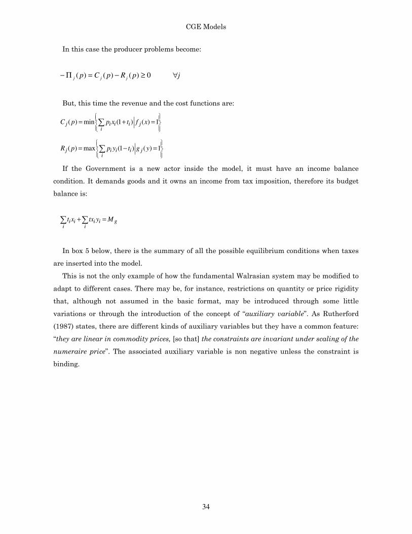
In this case the producer problems become:

0)()()( ≥−=Π− pRpCp jjj j∀

But, this time the revenue and the cost functions are:

( ) min (1 ) ( ) 1j i i i ji

C p p x t f x

= + =∑

( ) max (1 ) ( ) 1j i i i ji

R p p y t g y

= − =∑

If the Government is a new actor inside the model, it must have an income balance

condition. It demands goods and it owns an income from tax imposition, therefore its budget

balance is:

gi i i ii i

t x tx y M+ =∑ ∑

In box 5 below, there is the summary of all the possible equilibrium conditions when taxes

are inserted into the model.

This is not the only example of how the fundamental Walrasian system may be modified to

adapt to different cases. There may be, for instance, restrictions on quantity or price rigidity

that, although not assumed in the basic format, may be introduced through some little

variations or through the introduction of the concept of “auxiliary variable”. As Rutherford

(1987) states, there are different kinds of auxiliary variables but they have a common feature:

“they are linear in commodity prices, [so that] the constraints are invariant under scaling of the

numeraire price”. The associated auxiliary variable is non negative unless the constraint is

binding.

CGE Models

35

Non- linear complementarity problems are not enough to study the wide variety of different

assumptions on variables: they may be free, bound, or non-negative, for example.

Researchers have introduced and investigated a new class of problems, the MCP (Mixed

Complementarity Problem), which, using Ferris’s and Kanzow’s (1998) words, may be

described in the following way: the problem may be reduced to find a vector ,x l u ∈ such that

exactly one of the following holds:

i ix l= and ( ) 0iF x >

i iux = and ( ) 0iF x <

,i i il ux ∈ and ( ) 0i xF =

To conclude and compare the standard traditional format for CGE and the MCP format, we

present the two archetype economies already shown in box 1. However, this time the

fundamental relations are expressed in the new format.

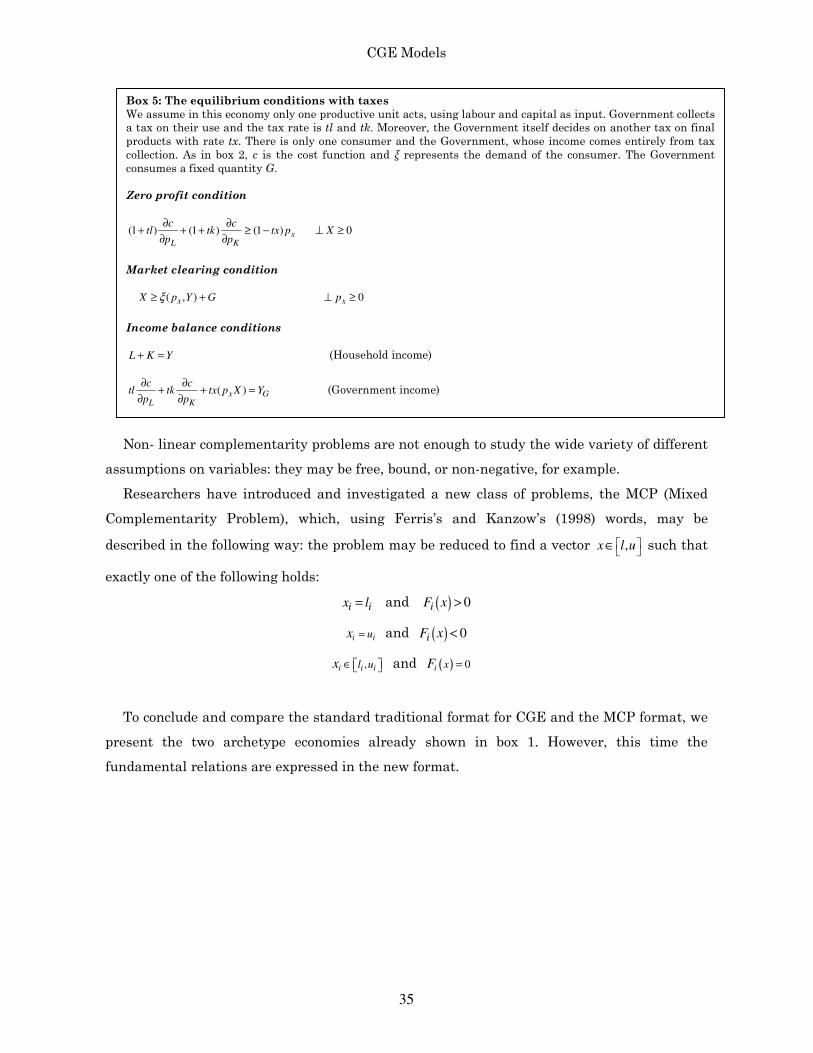
Box 5: The equilibrium conditions with taxes

We assume in this economy only one productive unit acts, using labour and capital as input. Government collects

a tax on their use and the tax rate is tl and tk. Moreover, the Government itself decides on another tax on final

products with rate tx. There is only one consumer and the Government, whose income comes entirely from tax

collection. As in box 2, c is the cost function and ξ represents the demand of the consumer. The Government

consumes a fixed quantity G.

Zero profit condition

(1 ) (1 ) (1 ) xL K

c ctl tk tx p

p p

∂ ∂+ + + ≥ −

∂ ∂ 0X⊥ ≥

Market clearing condition

( , )xX p Y Gξ≥ + 0xp⊥ ≥

Income balance conditions

L K Y+ = (Household income)

( )x GL K

c ctl tk tx p X Y

p p

∂ ∂+ + =

∂ ∂ (Government income)

CGE Models

36

V. The Mathematical Programming System for General Equilibrium (MPSGE)

Formally, General Equilibrium remains the same in both the standard format and in the

MCP (Mixed Complementarity Problem) format. The three basic relations that characterize an

equilibrium are the same and the same role is played by the fundamental variables. This

evolution in GE representation has been a great gain.

As we have already discussed, GEs are implemented in the real World to evaluate policies

and economic shocks. In this way they become AGE, or Applied General Equilibrium models.

They are usually large - scale models, and are more complicated than theoretical ones.

Modellers need a tool in order to implement their models and have quantitative results. In

the late 1980s GAMS (General Algebraic Modelling System) became available for the economic

community, after having been a tool only at the World Bank since 1983 (when Meeraus

developed this programming language). It was a program useful for solving a wide variety of

mathematical problems and one of its applications was on GE. However, its structure and its

Box 6: The translation of CGE in box 1 into MCP format

Here, we present the MCP version of the CGEs presented in box 1. The theoretical assumptions are the same.

We only note that in this case we manifestly implement that the share of each consumer’s savings respect to

total private savings is constant. Here we only translate the model into a Mixed Complementarity Problem

highlighting the constraints and the conditions for equilibrium.

A STANDARD CLOSED ECONOMY

WITHOUT GOVERNMENT

A STANDARD CLOSED ECONOMY WITH

GOVERNMENT

Zero profit condition Zero profit condition

( )1w r G PX

ββ −⋅ = =

( )1w r G PX

ββ −⋅ = =

Market clearing conditions Market clearing conditions

( )( )/GDP G WORK RENT PX INV= = + + ( )( )/GDP G WORK RENT GOVT PX INV= = + + +

( )1r

LS G GDPw

β

β−

= = ⋅ ⋅

( )1r

LS G GDPw

β

β−

= = ⋅ ⋅

(1 )r

KS G GDPw

β

β

= = ⋅ − ⋅

(1 )r

KS G GDPw

β

β

= = ⋅ − ⋅

Income balance conditions Income balance conditions

( )WORK E wLS alphaz PX INV= = − ⋅ (1 ) ( )WORK E wLS tw alphaz PX INV= = − − ⋅ (1 )( )RENT E rKS alphaz PX INV= = − − ⋅ (1 ) (1 )( )rRENT E rKS t alphaz PX INV= = − − − ⋅

( )r wGOVT E t KS t LS PX GSAV= = ⋅ + − ⋅

Accounting check Accounting check (1 )wWORK L s w LS= = − ⋅ ⋅ ( )(1 ) (1 )w wWORK L s w LS t= = − ⋅ ⋅ −

(1 )rRENT L s rKS= = − ⋅ ( )(1 ) (1 )r rRENT L s r kS t= = − ⋅ ⋅ −

GDP= real production, LD= labour demand, KD= capital demand, LS= labour supply, KS= capital supply,

r= rental rate of capital, w=wage rate, WORK= nominal workers’ consumption, RENT= nominal

capitalists’ consumption, sw= saving propensity for workers, sr= saving propensity for capitalists, INV=

real investments, PX= output price, GOVT= nominal government consumption, tw= direct tax rate on

workers, tr= direct tax rate on capitalists, GSAV= nominal government saving.

= G = means greater than, = E = means strictly equal, and = L = means lower than.

CGE Models

37

rules make it too complicated to employ for large- scale models16. Therefore, in 1987

Rutherford created a new tool which he thought may be useful in the GAMS framework but

which was specifically for GE problems. As the author himself declared: “MPSGE is a

language for concise representation of Arrow- Debreu economic equilibrium models. […]

MPSGE provides a short-hand representation for the complicated system of non-linear

inequalities which underlie general equilibrium models. The MPSGE framework is based on

nested constant elasticity of substitution utility functions and production functions, the data

requirements for a model include hare and elasticity parameters, endowments, and tax rates for

all the consumers and production sectors included in the model”. Rutherford (2005) asserts

that these two programs have different philosophies: “MPSGE was (and is) appropriate for a

specific class of nonlinear equations, while GAMS is capable of representing any system of

algebraic equations”.

The great innovation of this system is double. It is an interface of GAMS. Indeed

contemporaneously modellers may exploit the easier data handling and report writing

facilities of GAMS and the lower data requirement of MPSGE17. It is also a system that

“thinks” like an economist. It is not only able to solve mathematical systems but it organizes

data according to an MCP. This is the innovation: having demonstrated that the Arrow-

Debreu model may have at least two different formal representations, Rutherford has built a

program which reconstructs the complementarity conditions as we have presented them in the

previous paragraph. To empirically demonstrate these statements, we present in boxes 6 and

7 both the GAMS and the MPSGE versions of a simple program. We should demonstrate

firstly that the GAMS version is time- consuming while in MPSGE is less so in writing down

the program. Secondly, GAMS requires the extensive written record of all the equalities and

inequalities. MPSGE automatically recognizes CES function (and nested CES functions). It is

sufficient to point out the function and the elasticity of substitution (which is a piece of

information, we can say, on the slope of the curve) thus MPSGE recognizes exactly which of

the infinite CES functions is the correct one. It is evident that both programs run the MCP

solver because the solution statement is common, as is the variable declaration in both cases.

Referring to the examples, at first glance the reader may rebut our thesis and say that

GAMS code is shorter and therefore it requires less time to be written. If we count the lines of

the codes (54 against 75) this rebut is correct, but if we analyse the contents of the model, the

16 To have information on the features of GAMS, see Rosenthal’s (2008) user’s guide.

17 Using the words of its inventor: “the interface between GAMS and MPSGE combines the strengths of

both programs. The system uses GAMS as the “front end” and the “back end” to MPSGE, facilitating

data handling and report writing. The language employs an extended MPSGE syntax based on GAMS

sets, so that model specification is concise” (Rutherford, 2005).

CGE Models

38

great advantages of the MPSGE code are clear. The fundamental element is the definition of

equilibrium conditions. In GAMS the modeller has to write down the whole functional form of

each condition. In our example, which has only an illustrative aim, the chosen functions are

simple: Cobb-Douglas production functions. Many times, there are more complex functions,

even multistage functions. In these cases, writing down the functional form is time consuming

and prone to error. In MPSGE, functions are not required to be written extensively because it

is sufficient to give limited information and the program is already able to solve the problem.

What we need is only the benchmark data.

This advantage makes MPSGE useful both for experts and novice modellers: “the expert

knowledge embodied in MPSGE is of particular use to economists who are interested in the

insight provided by formal models but who are unable to devote many hours to programming.

MPSGE provides a structured framework for novice modellers. When used by experts, MPSGE

reduces the setup cost of producing an operational model and the cost of producing an

operational model and the cost of testing alternative specifications” (Rutherford, 2005).

Box 7: The GAMS code for the solution of an illustrative CGE $TITLE: SIMPLE CGE IN GAMS

Parameters

sw Worker propensity to save

sr Rentier propensity to save

alphaz Worker savings share on total savings

INV Exogenous real investment level

;

sw=0.125;

sr=0.25;

alphaz=0.25;

INV = 100*(sw*(40/100)+sr*(60/100)) ;

Positive Variables

V Acivity level for productive sector

Q Price index for commodity (value added)

r Profit rate

w Wage rate

WORK Consumer Expenditures

RENT Rentier Expenditures

Equations

ZPC_V Zero profit condition productive sector

MC_V Market clearing commodity

MC_L Market clearing factor L

MC_K Market clearing commodity K

IWORK Worker expenditures

IRENT Rentier expenditures;

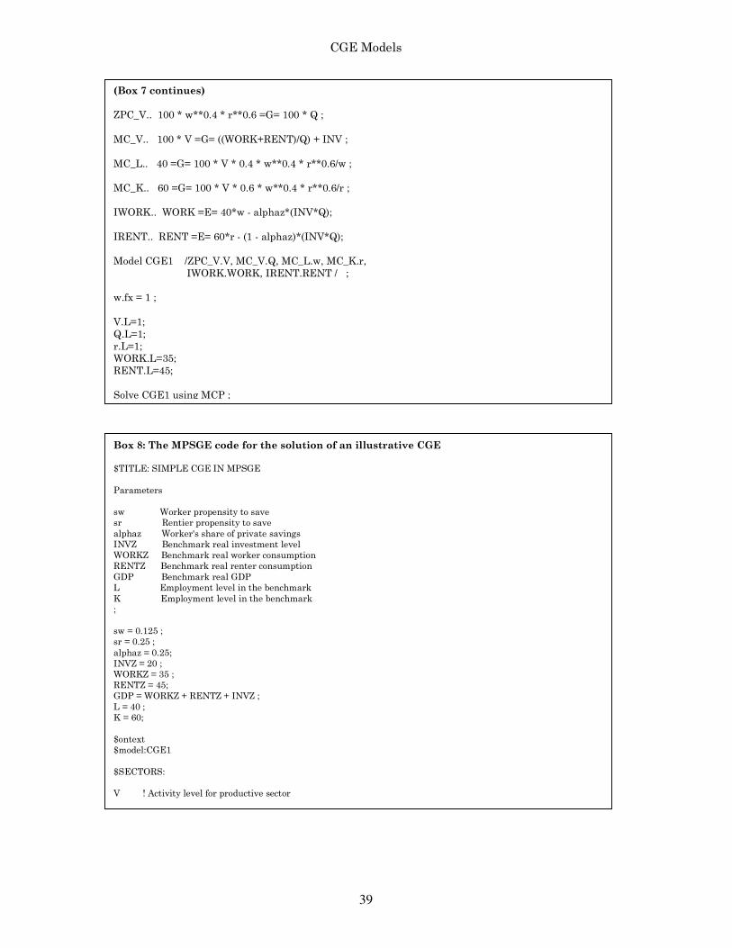
CGE Models

39

Box 8: The MPSGE code for the solution of an illustrative CGE

$TITLE: SIMPLE CGE IN MPSGE

Parameters

sw Worker propensity to save

sr Rentier propensity to save

alphaz Worker's share of private savings

INVZ Benchmark real investment level

WORKZ Benchmark real worker consumption

RENTZ Benchmark real renter consumption

GDP Benchmark real GDP

L Employment level in the benchmark

K Employment level in the benchmark

;

sw = 0.125 ;

sr = 0.25 ;

alphaz = 0.25;

INVZ = 20 ;

WORKZ = 35 ;

RENTZ = 45;

GDP = WORKZ + RENTZ + INVZ ;

L = 40 ;

K = 60;

$ontext

$model:CGE1

$SECTORS:

V ! Activity level for productive sector

(Box 7 continues)

ZPC_V.. 100 * w**0.4 * r**0.6 =G= 100 * Q ;

MC_V.. 100 * V =G= ((WORK+RENT)/Q) + INV ;

MC_L.. 40 =G= 100 * V * 0.4 * w**0.4 * r**0.6/w ;

MC_K.. 60 =G= 100 * V * 0.6 * w**0.4 * r**0.6/r ;

IWORK.. WORK =E= 40*w - alphaz*(INV*Q);

IRENT.. RENT =E= 60*r - (1 - alphaz)*(INV*Q);

Model CGE1 /ZPC_V.V, MC_V.Q, MC_L.w, MC_K.r,

IWORK.WORK, IRENT.RENT / ;

w.fx = 1 ;

V.L=1;

Q.L=1;

r.L=1;

WORK.L=35;

RENT.L=45;

Solve CGE1 using MCP ;

CGE Models

40

Therefore, defining general equilibrium as an MCP is not only a theoretical innovation but

it is translated into a new instrument for empirical analysis18.

Here, we present the main features of this system since we will employ it in our further

simulations. We will start with the benchmark, how to build it and its importance, and then

move on to the syntax.

Like any tool used for policy evaluation, we need an initial benchmark to calibrate our

model; to check the benchmark replication in order to affirm that the system is well written

and ready to be employed for analysis. Any AGE requires a benchmark that is commonly

represented by a SAM (Social Accounting Matrix), which in a compact format (a square

18 Although the theoretical foundation of MPSGE is the MCP representation of general equilibrium, the

evolution of MPSGE requires another innovation: the SLCP (Sequence of Linear Complementarity

Problems) algorithm, created by Mathiesen in 1985. For information see Mathiesen (1985, 1987).

(Box 8 continues)

$COMMODITIES:

Q ! Price index for commodity

r ! Profit rate

w ! Wage rate

$CONSUMERS:

WORK ! Worker expenditures

RENT ! Renter expenditures

$PROD:V s:1

O:Q Q:GDP

I:r Q:K

I:w Q:L

$DEMAND:WORK

D:Q Q:WORKZ

E:Q Q:(-(alphaz*(INVZ)))

E:w Q:L

$DEMAND:RENT

D:Q Q:RENTZ

E:Q Q:(-(1-alphaz)*(INVZ))

E:r Q:K

$REPORT:

V:RWORK D:Q DEMAND:WORK

V:RRENT D:Q DEMAND:RENT

V:RGDP O:Q PROD:V

V:EL I:w PROD:V

$offtext

$sysinclude mpsgeset CGE1

$include CGE1.gen

Solve CGE1 using MCP;

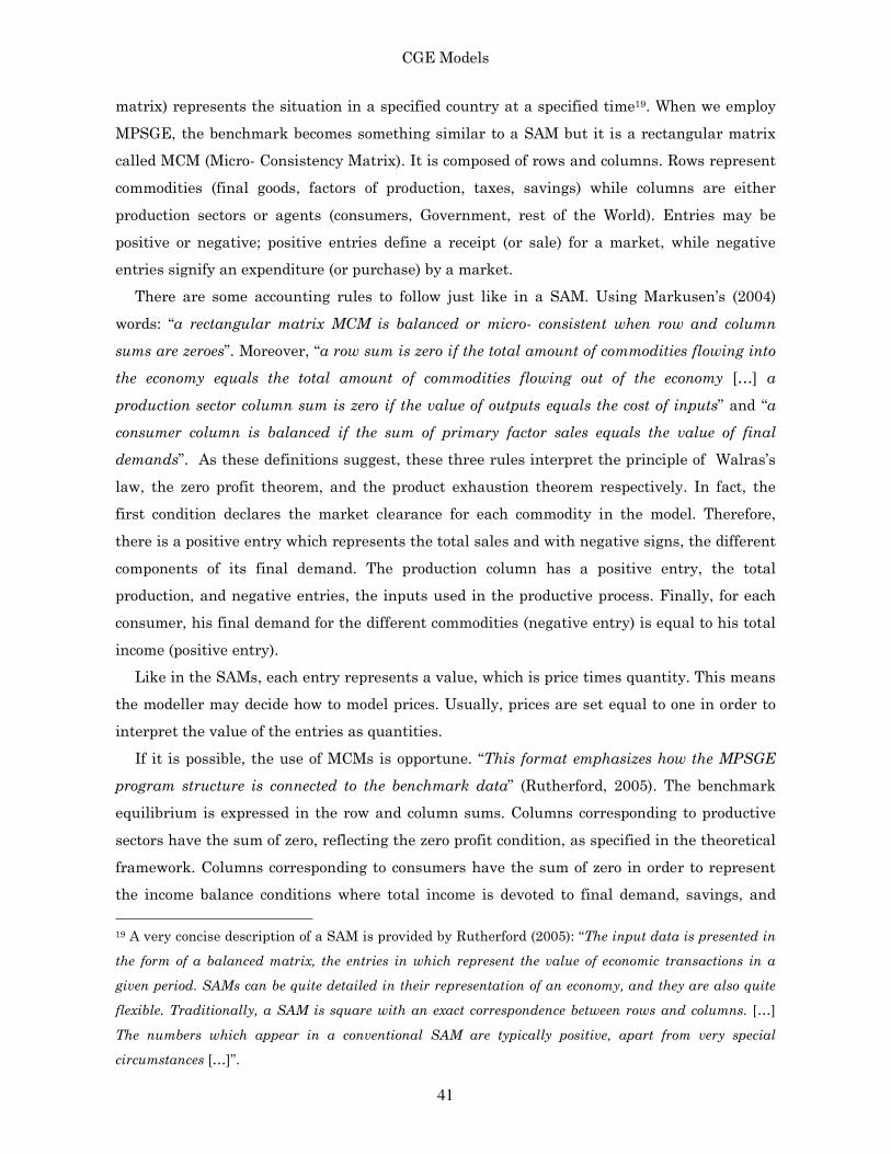
CGE Models

41

matrix) represents the situation in a specified country at a specified time19. When we employ

MPSGE, the benchmark becomes something similar to a SAM but it is a rectangular matrix

called MCM (Micro- Consistency Matrix). It is composed of rows and columns. Rows represent

commodities (final goods, factors of production, taxes, savings) while columns are either

production sectors or agents (consumers, Government, rest of the World). Entries may be

positive or negative; positive entries define a receipt (or sale) for a market, while negative

entries signify an expenditure (or purchase) by a market.

There are some accounting rules to follow just like in a SAM. Using Markusen’s (2004)

words: “a rectangular matrix MCM is balanced or micro- consistent when row and column

sums are zeroes”. Moreover, “a row sum is zero if the total amount of commodities flowing into

the economy equals the total amount of commodities flowing out of the economy […] a

production sector column sum is zero if the value of outputs equals the cost of inputs” and “a

consumer column is balanced if the sum of primary factor sales equals the value of final

demands”. As these definitions suggest, these three rules interpret the principle of Walras’s

law, the zero profit theorem, and the product exhaustion theorem respectively. In fact, the

first condition declares the market clearance for each commodity in the model. Therefore,

there is a positive entry which represents the total sales and with negative signs, the different

components of its final demand. The production column has a positive entry, the total

production, and negative entries, the inputs used in the productive process. Finally, for each

consumer, his final demand for the different commodities (negative entry) is equal to his total

income (positive entry).

Like in the SAMs, each entry represents a value, which is price times quantity. This means

the modeller may decide how to model prices. Usually, prices are set equal to one in order to

interpret the value of the entries as quantities.

If it is possible, the use of MCMs is opportune. “This format emphasizes how the MPSGE

program structure is connected to the benchmark data” (Rutherford, 2005). The benchmark

equilibrium is expressed in the row and column sums. Columns corresponding to productive

sectors have the sum of zero, reflecting the zero profit condition, as specified in the theoretical

framework. Columns corresponding to consumers have the sum of zero in order to represent

the income balance conditions where total income is devoted to final demand, savings, and

19 A very concise description of a SAM is provided by Rutherford (2005): “The input data is presented in

the form of a balanced matrix, the entries in which represent the value of economic transactions in a

given period. SAMs can be quite detailed in their representation of an economy, and they are also quite

flexible. Traditionally, a SAM is square with an exact correspondence between rows and columns. […]

The numbers which appear in a conventional SAM are typically positive, apart from very special

circumstances […]”.

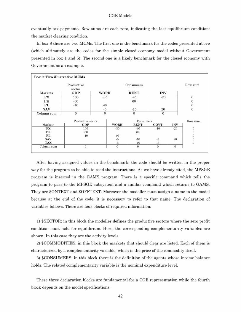
CGE Models

42

eventually tax payments. Row sums are each zero, indicating the last equilibrium condition:

the market clearing condition.

In box 8 there are two MCMs. The first one is the benchmark for the codes presented above

(which ultimately are the codes for the simple closed economy model without Government

presented in box 1 and 5). The second one is a likely benchmark for the closed economy with

Government as an example.

After having assigned values in the benchmark, the code should be written in the proper

way for the program to be able to read the instructions. As we have already cited, the MPSGE

program is inserted in the GAMS program. There is a specific command which tells the

program to pass to the MPSGE subsystem and a similar command which returns to GAMS.

They are $ONTEXT and $OFFTEXT. Moreover the modeller must assign a name to the model

because at the end of the code, it is necessary to refer to that name. The declaration of

variables follows. There are four blocks of required information:

1) $SECTOR: in this block the modeller defines the productive sectors where the zero profit

condition must hold for equilibrium. Here, the corresponding complementarity variables are

shown. In this case they are the activity levels.

2) $COMMODITIES: in this block the markets that should clear are listed. Each of them is

characterized by a complementarity variable, which is the price of the commodity itself.

3) $CONSUMERS: in this block there is the definition of the agents whose income balance

holds. The related complementarity variable is the nominal expenditure level.

These three declaration blocks are fundamental for a CGE representation while the fourth

block depends on the model specifications.

Box 9: Two illustrative MCMs

Productive

sector

Consumers Row sum

Markets GDP WORK RENT INV

PX 100 -35 -45 -20 0

PK -60 60 0

PL -40 40 0

SAV -5 -15 20 0

Column sum 0 0 0 0

Productive sector Consumers Row sum

Markets GDP WORK RENT GOVT INV

PX 100 -30 -40 -10 -20 0

PK -60 60 0

PL -40 40 0

SAV -5 -10 -5 20 0

TAX -5 -10 15 0

Column sum 0 0 0 0 0

CGE Models

43

4) $AUXILIARY: in this case we must employ the definition of auxiliary variables when

want to model constraints or non - Walrasian systems.

After the declaration of sectors and variables, the program requires us to assign values to

each block. The key element is $PROD: when we want to assign values for a productive sector,

and $DEMAND: when we want to assign values for each consumer. Let us now describe firstly

the $PROD: block. The first line includes the command, the name of the productive sector and

the elasticity of substitution between inputs, and elasticity of transformation when a

combined production in a single sector occurs. Then the second line includes three fields; the

O: field refers to which one is the produced commodity, Q: is the field for the produced

quantity and P: is the price. We may read this line as follows: “the sector whose output is a

commodity such that its price is what we have fill in the O: field and whose quantity is inserted

in the Q: field. Then, its final price is the one in P:”. The following lines are quite similar but

the first field is now I: which stands for inputs.

As an example, in box 7, the productive sector is called V and produces a commodity whose

price is Q. The final production is 100. There is not any P: field since we assume the default

value to be 1. To produce that good, the sector employs two inputs whose prices are r and w in

quantities 60 and 40 respectively. There is no elasticity of substitution between inputs because

we assume a Cobb - Douglas function whose elasticity is unitary (one is the default value).

The $DEMAND: block should be referred to an agent in the first line. Then, in the D: field

there is the price of the demanded commodity and in Q:, the related quantity. In the following

lines the first field is the E: field, which means endowments, and then as usual the Q: field is

where the quantity is inserted.

In our example there are two $DEMAND: blocks one for workers and one for renters but

both of them present the same scheme: the definition of the agent ($DEMAND:WORK,

$DEMAND:RENT), the definition of the demands (D:Q Q:WORKZ and D:Q Q:RENTZ), and

the definition of the endowments (E:Q Q:(-(alphaz*(INVZ))), E:w Q:L, E:Q Q:(-(1-

alphaz)*(INVZ)), and E:r Q:K).

This block may be read in this way: “there is an agent who demands for a good whose price

is in the D: field in quantity Q: field. He is endowed with commodities whose prices are in E:

fields and in quantity Q: fields”.

If an $AUXILIARY: block has been defined, there should be a $CONSTRAINT:, an equation

that is set to give a value to the auxiliary variable. It must be written in GAMS language.

Finally, a useful tool is the $REPORT: block. It is not necessary to solve the model but it

could be useful in the output file. In fact, in this block we build a variable V: which refers to

one of the variables we have used before. For example, in the box above, in the report file we

CGE Models

44

have created a variable whose name is RGDP, which means real GDP. But we must tell the

program where to find this value. In this case we say: “go to the output field of a commodity

whose price is Q in the producer block PROD:V”. Therefore, in the output file these useful

values are directly shown.