Computable General Equilibrium Models

and Their Use in Economy-Wide Policy Analysis:

Everything You Ever Wanted to Know (But Were Afraid to Ask)

Ian Sue Wing*

Center for Energy & Environmental Studies and Department of Geography & Environment

Boston University

and

Joint Program on the Science & Policy of Global Change

Massachusetts Institute of Technology

* Address: Rm. 141, 675 Commonwealth Ave., Boston MA 02215. Email: isw@bu.edu. Phone: (617) 353-5741. Fax: (617) 353-5986. This research was supported by U.S. Department of Energy Office of Science (BER) Grant No. DE-FG02-02ER63484.

Computable General Equilibrium Models

and Their Use in Economy-Wide Policy Analysis:

Everything You Ever Wanted to Know (But Were Afraid to Ask)

Abstract

This paper is a simple, rigorous, practically-oriented exposition of computable general

equilibrium (CGE) modeling. The general algebraic framework of a CGE model is developed

from microeconomic fundamentals, and employed to illustrate (i) how a model may be calibrated

using the economic data in a social accounting matrix, (ii) how the resulting system of numerical

equations may be solved for the equilibrium values of economic variables, and (iii) how

perturbing this equilibrium by introducing tax or subsidy distortions facilitates analysis of

policies’ economy-wide impacts.

JEL Classification: C68, D58, H22, Q43

Keywords : general equilibrium, CGE models, policy analysis, taxation

1

1. Introduction

Walrasian general equilibrium prevails when supply and demand are equalized across all of the

interconnected markets in the economy. Computable general equilibrium (CGE) models are

simulations that combine the abstract general equilibrium structure formalized by Arrow and

Debreu with realistic economic data to solve numerically for the levels of supply, demand and

price that support equilibrium across a specified set of markets. CGE models are a standard tool

of empirical analysis, and are widely used to analyze the aggregate welfare and distributional

impacts of policies whose effects may be transmitted through multiple markets, or contain menus

of different tax, subsidy, quota or transfer instruments. Examples of their use may be found in

areas as diverse as fiscal reform and development planning (e.g., Perry et al 2001; Gunning and

Keyzer 1995), international trade (e.g., Shields and Francois 1994; Martin and Winters 1996;

Harrison et al 1997), and increasingly, environmental regulation (e.g., Weyant 1999; Bovenberg

and Goulder 1996; Goulder 2002).

CGE models’ usefulness notwithstanding, they are nonetheless viewed with suspicion by some

in the economics and policy analysis communities as a “black box” , whose results cannot be

meaningfully traced to any particular features of their data base or input parameters, algebraic

structure, or method of solution. Such criticism typically rests on the presumptions that CGE

models contain a large number of variables and parameters and are structurally complex, both of

which allow questionable assumptions to be hidden within them that end up driving their results.

A good example is Panagariya and Duttagupta (2001), who note in the context of trade

liberalization that:

2

“Unearthing the features of CGE models that drive [their results] is often a time-

consuming exercise. This is because their sheer size, facilitated by recent

advances in computer technology, makes it difficult to pinpoint the precise source

of a particular result. They often remain a black box. Indeed, frequently, authors

are themselves unable to explain their results intuitively and, when pressed, resort

to uninformative answers...”

While this view contains a kernel of truth, it is also symptomatic of misunderstanding of the

simplicity of the algebraic foundation at the core of all CGE models—regardless of their size or

apparent complexity, the key features of the data that these models use, the numerical calibration

methods by which models employ these data to imbue their algebraic framework with empirical

substance, and the operations research techniques by which the resulting mathematical

programming problem is solved to generate the results that are then quoted in the policy

literature.

The problem is that much of this information is often not communicated in manner that is

accessible to the broader economics or policy communities. Descriptions of models’ underlying

structure, calibration and solution methods abound, but tend to be spread across a broad cross-

section of materials, each of subset of which focuses on a different aspect of the subject. Of the

numerous articles that use CGE simulations, the majority document only those attributes of their

models that are relevant to the application at hand (e.g., Jacoby and Sue Wing 1998), or merely

present the model’s equations with little explanation to accompany them (e.g., Bovenberg and

Goulder 1996). Expositions in books and manuals devoted to modeling techniques (e.g., Shoven

and Whalley 1992; Ginsburgh and Keyzer 1997; Lofgren et al 2002) tend to be exhaustively

3

detailed, and those in articles focused on applied numerical optimization (e.g., Rutherford 1995;

Ferris and Pang 1997) often involve a high level of mathematical abstraction, neither of which

make it easy for the uninitiated to quickly grasp the basics. Finally, although pedagogic articles

(e.g., Devarajan et al 1997; Rutherford 1999; Rutherford and Paltsev 1999; Paltsev 2004) often

provide a lucid introduction to the fundamentals, they tend to emphasize either models’ structural

descriptions or the details of the mathematical software packages used to build them, and have

given short shrift to CGE models’ theoretical basis or procedures for calibration.

It is therefore difficult to find an article-length introduction to the subject that integrates these

disparate elements into a practical, intuitive explanation of the methods by which CGE models

are constructed, calibrated, solved, and used to analyze the impacts of policies with economy-

wide effects.1 This gap in the literature motivates the present paper, whose aim is to de-mystify

CGE models by opening up the black box to scrutiny, and to increase their accessibility to a

wider group of economists and policy analysts—students, practitioners and academics alike—

who would otherwise remain unfamiliar with, and suspicious of, them.

In line with its pedagogical objective, the paper is deliberately simple. In the spirit of Shoven and

Whalley (1984), Kehoe and Kehoe (1995), and Kehoe (1998a), it employs the microeconomic

foundations of consumer and producer maximization to develop a framework that is not just

straightforward but is also sufficiently general to represent a CGE model of arbitrary size and

dimension. This framework is then used to demonstrate in a practical fashion how a social

accounting matrix may be used to calibrate the coefficients of the model equations, how the

1 But see recent exceptions by Kehoe (1998a) and Boehringer et al (2003).

4

resulting system of numerical equations is solved, and how the equilibrium thus solved for may

be perturbed and the results used to analyze the economic effects of policies.

To specialists who are already familiar with CGE models, there will be little in this paper that is

new, as the aforementioned techniques of model formulation, specification, calibration and

solution are all well established. The primary contribution of the paper is the framework that it

develops to integrate these elements in a transparent and step-by-step manner, creating a

pedagogic digest that can serve as an introduction to the subject of CGE modeling that is simple

and practically oriented, yet also theoretically coherent and reasonably comprehensive. The hope

is that this will not only alleviate some of the general suspicion about CGE models, but will also

facilitate and promote their use as a tool for policy analysis by giving the reader an appreciation

of their simplicity and power.

The plan of the paper is as follows. Section 2 introduces the circular flow of the economy, and

demonstrates how it serves as the fundamental conceptual starting point for Walrasian

equilibrium theory that underlies a CGE model. Section 3 presents a social accounting matrix

and shows how the algebra of its accounting rules reflects the conditions of general equilibrium.

Section 4 develops these relationships into a CGE model using the device of the Cobb-Douglas

(C-D) economy in which households have C-D preferences and firms have C-D production

technology. Section 5 discusses techniques of model formulation, solution and numerical

calibration. Section 6 explains the use of CGE models to analyze the incidence and welfare

effects of taxes, and section 7 provides a practical demonstration using a stylized numerical

example. A more realistic example is presented in section 8, which applies a CGE simulation of

5

the C-D economy to U.S. data for the purpose of elucidating the general equilibrium effects of

taxing carbon dioxide emissions to mitigate global warming. Section 9 provides a summary and

conclusion.

2. Foundations: The Circular Flow and Walrasian Equilibrium

The fundamental conceptual starting point for a CGE model is the circular flow of commodities

in a closed economy, shown in Figure 1.2 The main actors in the diagram are households, who

own the factors of production and are the final consumers of produced commodities, and firms,

who rent the factors of production from the households for the purpose of producing goods and

services that the households then consume. Many CGE models also explicitly represent the

government, but its role in the circular flow is often passive: to collect taxes and disburse these

revenues to firms and households as subsidies and lump-sum transfers, subject to rules of

budgetary balance that are specified by the analyst. In tracing the circular flow one can start with

the supply of factor inputs (e.g. labor and capital services) to the firms and continue to the supply

of goods and services from the firms to the households, who in turn control the supply of factor

services. One may also begin with payments, which households receive for the services of labor

and capital provided to firms by their primary factor endowment, and which are then used as

income to pay producing sectors for the goods and services that the households consume.

Equilibrium in the economic flows in Figure 1 results in the conservation of both product and

value. Conservation of product, which holds even when the economy is not in equilibrium,

reflects the physical principle of material balance that the quantity of a factor with which

households are endowed, or of a commodity that is produced by firms, must be completely

6

absorbed by the firms or households (respectively) in the rest of the economy. Conservation of

value reflects the accounting principle of budgetary balance that for each activity in the economy

the value of expenditures must be balanced by the value of incomes, and that each unit of

expenditure has to purchase some amount of some type of commodity. The implication is that

neither product nor value can appear out of nowhere: each activity’s production or endowment

must be matched by others’ uses, and each activity’s income must be balanced by others’

expenditures. Nor can product or value disappear: a transfer of purchasing power can only be

effected through an opposing transfer of some positive amount of some produced good or

primary factor service, and vice versa.

These accounting rules are the cornerstones of Walrasian general equilibrium. Conservation of

product, by ensuring that the flows of goods and factors must be absorbed by the production and

consumption activities in the economy, is an expression of the principle of no free disposability.

It implies that firms’ outputs are fully consumed by households, and that households’

endowment of primary factors is in turn fully employed by firms. Thus, for a given commodity

the quantity produced must equal the sum of the quantities of that are demanded by the other

firms and households in the economy. Analogously, for a given factor the quantities demanded

by firms must completely exhaust the aggregate supply endowed to the households. This is the

familiar condition of market clearance.

Conservation of value implies that the sum total of revenue from the production of goods must

be allocated either to households as receipts for primary factors rentals, to other industries as

payments for intermediate inputs, or to the government as taxes. The value of a unit of each

2 This discussion is adapted from Babiker et al (2001).

7

commodity in the economy must then equal the sum of the values of all the inputs used to

produce it: the cost of the inputs of intermediate materials as well as the payments to the primary

factors employed in its production. The principle of conservation of value thus simultaneously

reflects constancy of returns to scale in production and perfectly competitive markets for

produced commodities. These conditions imply that in equilibrium producers make zero profit.3

Lastly, the returns to households’ endowments of primary factors, that are associated with the

value of factor rentals to producers, accrue to households as income that the households exhaust

on goods purchases. The fact that households’ factor endowments are fully employed, so that no

amount of any factor is left idle, and that households exhaust their income, purchasing some

amount of commodities—even for the purpose of saving, reflects the principle of balanced-

budget accounting known as income balance. One can also think of this principle as a zero profit

condition on the production of a “utility good”, whose value is the aggregate of the values of

households’ expenditures on commodities, and whose price is the marginal utility of income.

The three conditions of market clearance, zero profit and income balance are employed by CGE

models to solve simultaneously for the set of prices and the allocation of goods and factors that

support general equilibrium. The three conditions define Walrasian general equilibrium not by

the process of exchange by which this allocation comes about, but in terms of the allocation

itself, which is made up of the components of the circular flow shown by solid lines in Figure 1.

General equilibrium can therefore be modeled in terms of barter trade in commodities and

factors, without the need to explicitly keep track of—or even represent—the compensating

3 Together, these conditions imply that with unfettered competition firms will continue to enter the economy’s markets for goods until profits are competed away to zero.

8

financial transfers. Consequently, CGE models typically do not explicitly represent money as a

commodity. However, in order to account for such trades the quantities of different commodities

still need to be made comparable by denominating their values in some common unit of account.

The flows are thus expressed in terms of the value of one commodity—the so-called numeraire

good—whose price is taken as fixed. For this reason, CGE models only solve for relative prices.

This point is elaborated later on in Section 4.

3. The Algebra of Equilibrium and the Social Accounting Matrix

The implications of the circular flow for both the structure of CGE models and the economic

data on which they are calibrated are clearly illustrated in an algebraic framework. To this end,

consider a hypothetical closed free-market economy that is composed of N industries, each of

which produces its own type of commodity, and an unspecified number of households that

jointly own an endowment of F different types of primary factors.

To keep things simple we make three assumptions about this economy. First, there are no tax or

subsidy distortions, or quantitative restrictions on trade. Second, the households act collectively

as a single representative agent who rents out the factors to the industries in exchange for

income. Households then spend the latter to purchase the N commodities for the purpose of

satisfying D types of demands (e.g., demands for goods for the purposes of consumption and

investment). Third, each industry behaves as a representative firm that hires inputs of the F

primary factors and uses quantities of the N commodities as intermediate inputs to produce a

quantity y of its own type of output.

9

Then, letting the indices i = {1, ..., N} denote the set of commodities, j = {1, ..., N} the set of

industry sectors, f = {1, ..., F} the set of primary factors, and d = {1, ..., D} the set of final

demands, the circular flow in this economy can be completely characterized by three data

matrices: an N × N input-output matrix of industries’ uses of commodities as intermediate inputs,

denoted by X , an F × N matrix of primary factor inputs to industries, denoted by V , and an N ×

D matrix of commodity uses by final demand activities, denoted by G .

It is straightforward to establish how the elements of the three matrices may be arranged to

reflect the logic of the circular flow. First, commodity market clearance implies that the value of

gross output of industry i, which is the value of the aggregate supply of the ith commodity, iy ,

must equal the sum of the values of the j intermediate uses of that good, ijx , and the d final

demands idg that absorb that commodity:

(1) ��==

+=D

did

N

jiji gxy

11

.

Similarly, factor market clearance implies that the firms in the economy fully employ the

representative agent’s endowment of a particular factor, fV :

(2) �=

=N

ifjf vV

1

.

Second, the fact that industries make zero profit implies that the value of gross output of the jth

sector, jy , must equal the sum of the benchmark values of inputs of the i intermediate goods ijx

and f primary factors fjv that the industry employs in its production:

(3) ��==

+=F

ifj

N

iijj vxy

11

.

10

Third, the representative agent’s income, m , is made up of the receipts from the rental of

primary factors—none of which remain idle, and must balance the agent’s gross expenditure on

satisfaction of commodity demands. Together, these conditions imply that income must equal the

sum of the elements of V , which in turn must equal the sum of the elements of G . Thus, by eq.

(2),

(4) ���= ==

==N

i

D

did

F

ff gVm

1 11

.

The accounting relationships in eqs. (1)-(4) jointly imply that, in order to reflect the logic of the

circular flow, the matrices X , V and G should be arranged according to Figure 2(a). This

diagram is an accounting tableau known as a social accounting matrix (SAM), which is a

snapshot of the inter-industry and inter-activity flows of value within an economy that is in

equilibrium in a particular benchmark period. The SAM is an array of input-output accounts that

are denominated in the units of value of the period for which the flows in the economy are

recorded, typically the currency of the benchmark year. Each account is represented by a row

and a column, and the cell elements record the payment from the account of a column to the

account of a row. Thus, an account’s components of income of (i.e., the value of receipts from

the sale of a commodity) appear along its row, and the components of its expenditure (i.e., the

values of the inputs to a demand activity or the production of a good) appear along its column

(King 1985).

The structure the SAM reflects the principle of double-entry book-keeping, which requires that

for each account, total revenue—the row total—must equal total expenditure—the column total.

11

This is apparent from Figure 2(a), where the sum across any row in the upper quadrants X and

G is equivalent to the expression for goods market clearance from eq. (1), and the sum across

any row in the south-west quadrant V is equivalent to the expressions for factor market

clearance from eq. (2). Likewise, the sum down any column of the left-hand quadrants X and V

is equivalent to the expression for zero-profit in industries from eq. (3). Furthermore, once these

conditions hold, the sums of the elements of the northeast and southwest quadrants ( G and V ,

respectively) should equal one another, which is equivalent to the income balance relationship

from eq. (4) that reflects the intuition that GDP (the aggregate of the components of expenditure)

is equal to value added (the aggregate of the components of income). The fact that these

properties are the expression of Walrasian general equilibrium makes the SAM an ideal data base

from which to construct a CGE model.

4. From a SAM to a CGE Model: The Cobb-Douglas Economy

CGE models’ algebraic framework results from the imposition of the axioms of producer and

consumer maximization on the accounting framework of the SAM. To illustrate this point we use

the pedagogic device of a “Cobb-Douglas economy” in which households are modeled as a

representative agent that is assumed to have C-D preferences and industry sectors are modeled as

representative producers that are assumed to have C-D production technologies.

4.1. Households

The treatment of households mirrors that in the previous section. Assume a representative agent

that maximizes utility U by choosing levels of consumption c of the N commodities in the

economy, subject to the constraints of her income, m, ruling commodity prices p. The agent may

12

also demand goods and services for purposes other than consumption—in the present example

saving s—which are assumed to be exogenous and constant. The agent’s problem is thus:

(5) ),,(max 1 Nc

ccUi

� subject to

�=

+=N

iiii scpm

1

)( .

We assume that the representative agent has C-D preferences, so that her utility function is

∏=

==N

iiCNC

iN cAcccAU1

2121 αααα� ,

with 11 =++ Nαα � . It is equivalent but advantageous to re-formulate this problem as one of

household production, in which the representative agent maximizes the “profit” from the

production of a “utility good” U whose output is generated by consumption, and whose price pU

is the marginal utility of aggregate consumption, which can be treated as the numeraire price in

the economy. Thus, eq. (5) is equivalent to the problem:

(6) �=

−N

iiiU

ccpUp

i 1

max

subject to the definition of utility above. Solving this problem yields the representative agent’s

demand function for the consumption of the ith commodity:4

(7) i

N

iii

ii p

spm

c

��

���

� −=

�=1α .

Rearranging this expression yields

��

���

� −=

�=

N

iii

iii

spm

pc

1

α , which indicates that the exponents of the

utility function may be interpreted as the shares of each commodity in the total value of

4 The details are given in Appendix A.

13

consumption. Other components of final demand (e.g., saving or investment) may be easily

handled as sinks for product that are directly specified as demand functions, or the agent’s utility

function may be extended to incorporate the representative agent’s preferences for other

categories of expenditure.

4.2. Producers

Each producer maximizes profit π by choosing levels of N intermediate inputs x and F primary

factors v to produce output y, subject to the constraint of its production technology φ. The jth

producer’s problem is thus:

(8) ��==

−−=F

ffjf

N

iijijjj

vxvwxpyp

fjij 11,

maxπ subject to

( )FjjNjjjj vvxxy ,,;,, 11 ��φ= .

Let each producer have C-D production technology, so that its production function φ(·) is a

recipe for combining inputs of intermediate goods and primary factors of the form

( )( ) ∏∏==

==F

ffj

N

iijjFNjj

fjijNN vxAvvvxxxAy11

21212121

γβγγγβββ�� ,

with 111 =+++++ NjjNjj γγββ �� . Solving the problem in (8) yields producer j’s demands

for intermediate inputs of commodities:5

(9) i

jjijij p

ypx β= ,

and its demands for primary factor inputs:

(10) f

jjfjfj w

ypv γ= .

14

Rearranging eqs. (9) and (10) yields jj

ijiij yp

xp=β and

jj

fjffj yp

vw=γ , respectively, showing that

similar to the demand for consumption goods above, the exponents of the Cobb-Douglas

production function represent the shares of their respective inputs to production in the value of

output.

4.3. General Equilibrium

Eqs. (7), (9) and (10) are the building blocks from which a CGE model is constructed. What bind

these elements together are the general equilibrium conditions that are developed algebraically in

section 3, which must be re-formulated for the Cobb-Douglas economy. Once these conditions

are properly specified, (7), (9) and (10) may be substituted into them to yield the actual equations

that a CGE model uses to solve for equilibrium.

In the C-D economy the conditions for general equilibrium are as follows. Market clearance

implies that the quantity of each commodity produced must equal the sum of the quantities of

that commodity demanded by the j producers in the economy as an intermediate input to

production, and by the representative agent as an input to consumption and saving activities.

Thus, eq. (1) becomes:

(11) ii

N

jiji scxy ++=�

=1

.

In addition, the quantities of primary factor f used by all producers must sum to the

representative agent’s endowment of that factor, Vf. From eq. (2) this condition implies:

5 The details are given in Appendix B.

15

(12) �=

=N

jfjf vV

1

.

Zero profit implies that the value of output generated by producer j must equal the sum of the

values of the inputs of the i intermediate goods and f primary factors employed in production.

This condition is easily deduced by setting the right-hand side of eq. (8) to zero and rearranging:

(13) ��==

−=F

ffjf

N

iijijj vwxpyp

11

,

which is the analogue of is eq. (3). Income balance implies that the income of the representative

agent must equal the value of producers’ payments to her for the use of the primary factors that

she owns and hires out. Thus, as in eq. (4):

(14) �=

=F

fff Vwm

1

.

With these four expressions in hand the equations that form the core of a CGE model may be

easily specified.

Assume for simplicity that the endowment of the representative agent is fixed at the instant in

time in which general equilibrium prevails. Then, substituting (7) and (9) into eq. (11), and (10)

into eq.(12) yields two excess demand vectors that define the divergence ∆C between supply and

demand in the market for each commodity and the divergence ∆F between supply and demand in

the market for each primary factor. The absolute values of both of these sets of differences are

minimized to zero in general equilibrium. There are N such excess demand equations for the

commodity market:

(15) iiii

N

jjj

F

fffi

N

jjjij

Ci ypspspVwyp −+��

�

����

�−+=∆ ���

=== 111

αβ

16

and F equations for the factor market:

(16) f

N

j f

jj

fjFf V

w

yp−=∆ �

=1

γ .

The zero profit condition implies that the absolute value of producers’ profits is minimized to

zero in general equilibrium. Thus, substituting eqs. (9) and (10) into the production function

allows us to write N pseudo-excess demand functions that specify the per-unit excess profit (i.e.

excess of price over unit cost) ∆�

in each industry sector:

(17) ( ) ( )∏∏==

−=∆F

ffjf

N

iijijjj

fjij wpAp11

// γβπ γβ .

Finally, the income balance condition (14) can be re-written in terms of the excess of income

over returns to the agent’s endowment of primary factors, ∆m:

(18) mVwF

fff

m −=∆ �=1

.

General equilibrium is thus the joint minimization of ∆C, ∆F, ∆�

and ∆m.

5. The Formulation, Calibration and Solution of a CGE Model

5.1. Model Formulation

The way in which a CGE model solves for an equilibrium can now be readily understood. To

obtain a solution, the model uses eqs. (15)-(18). These expressions are formulated a system of 2N

+ F equations in 2N + F unknowns: an N-vector of industry output- or “activity” levels

],,[ 1 Nyy �=y , an N-vector of commodity prices ],,[ 1 Npp �=p , an F-vector of primary

factor prices ],,[ 1 Fww �=w and a scalar income level m. The problem of finding the vector of

activity levels and prices that supports general equilibrium therefore consists of choosing values

for these variables to solve the problem

17

(19) 0z =)(ξ ,

in which ],,,[ ′= mywpz is the vector of stacked prices, activity levels and level of income, and

],,,[)( ′∆=⋅ mFC πξ ��� is the system of stacked pseudo-excess demand equations, which forms

the production-inclusive pseudo-excess demand correspondence of the economy.

Eq. (19) is the expression of general equilibrium in a complementarity format, so named because

of the important complementarity that exists between prices and excess demands, and between

activity levels and profits, and that is a critical feature of general equilibrium. For the equilibrium

above to be economically meaningful, prices, activity levels and income are all positive and

finite (0 � z < � ). In the limit, as z approaches zero, eqs. (15), (17) and (18) all approach zero,

and eq. (16) tends to –Vf , implying that 00V00 ≤′−= ]0,,,[)(ξ . If z* is a vector of prices and

activity and income levels that supports general equilibrium, it must be the case that 0 � z* and

�(z*) = 0. Thus, the problem in eq. (19) may be compactly re-specified as one of finding

(20) 0z ≥ subject to 0zz0z =′≥ )(,)( ξξ ,

which is a mathematical statement of Walras’ Law that the sum of the values of market demands

equal to the sum of the values of market supplies.6

5.2. Numerical Calibration Using the SAM

Even with a specification of preferences and technology that is as simple as the C-D, the problem

in eq. (20) is still highly non-linear, with the result that there is no closed-form analytical

solution for z. This is the reason for the “C” in CGE models: general equilibrium systems with

realistic utility and production functions must be calibrated on a SAM of the kind discussed in

6 See, e.g. Varian (1992: 343).

18

section 3, generating a numerical optimization problem that can be solved using optimization

techniques.

Numerical calibration is easily accomplished in the C-D economy. The crucial step in this regard

is to compare eqs. (1)-(4) with eqs. (11)-(14). The pairs (1) and (11), (2) and

(12), (3) and (13), and (4) and (14) exhibit a striking symmetry. In particular, the elements of

each pair are equivalent if � j = 0 (zero profit, which we assume), ijiji xxp = and fjfjf vvw = .

Therefore, a fundamental equivalence may be drawn between the equations in a CGE model and

the benchmark flows of value in a SAM by assuming that in the benchmark year all prices are

equal to unity.

The foregoing observation is the essence of the simplest calibration procedure by which a CGE

model is “fit” to the benchmark equilibrium recorded in a SAM.7 All prices are treated as index

numbers with a value of unity in the benchmark, and all value flows in the SAM are treated as

benchmark quantities. These assumptions allow the technical coefficients and elasticity

parameters of the utility and production functions to be solved for directly (Mansur and Whalley

1983):

(21) CiCi Gg /=α ,

(22) ��

���

�= ∏=

N

iiCCC

igGA1

α ,

7 For an alternative procedure, see Kehoe (1998a). In the general case a CGE model’s production and consumption technologies are neither Leontief nor Cobb-Douglas. Then, in order to calibrate the model the value of the elasticities of substitution must be assumed by the modeler, as there are more estimated parameters than model equations, making the calibration problem under-determined. The econometric approach to calibration (e.g., Jorgenson 1984) circumvents much of the potential ad-hocracy in this process, but is data intensive, requiring time-

19

(23) jijij yx /=β ,

(24) jfjfj yv /=γ ,

(25) ���

����

�= ∏∏

==

F

ffj

N

iijjj

fjij vxyA11

γβ ,

(26) iSi gs = ,

(27) ff VV =

and

(28) �=

=F

ffVm

1

.

Having specified these values for the model’s coefficients, solving the numerical problem in eq.

(20) will then set the quantities of the variables in the C-D economy equal to the values of the

corresponding flows in the SAM (i.e., ijij xx = , fjfj vv = and iCi gc = ), replicating the

benchmark equilibrium.8

5.3. The Solution of a CGE Model in a Complementarity Format

The calibration procedure transforms (20) into a square system of numerical equations known as

a nonlinear complementarity problem or NCP (Ferris and Pang, 1997), which may be solved

using algorithms that are now routinely embodied in modern, commercially-available software

systems for optimization.9 Mathiesen (1985a,b) and Rutherford (1987) describe the basic

series of social accounting matrices which are often not available. See Dawkins et al (2001) for an excellent survey of these issues. 8 This calibration technique is equivalent to expressing the utility and production functions in calibrated share form (see Boehringer et al 2003: Tables 1 and 2). 9 Foremost among these is the PATH solver (Dirkse and Ferris 1995). It is especially powerful when used in combination with other software tools such as the Generalized Algebraic Modeling System (GAMS) numerical language (Brooke et al. 1999) and the MPSGE pre-processing subsystem (Rutherford, 1995, 1999), which automatically calibrates the technical coefficients in equations (7), (9) and (10) based on a SAM provided by the

20

approach, which is similar to a Newton-type steepest-descent optimization algorithm (Kehoe

1991: 2068-2072). The algorithm iteratively solves a sequence of linear complementarity

problems or LCPs (Cottle et al 1992), each of which is a first-order Taylor series expansion of

the non-linear function �. The LCP solved at each iteration is thus one of finding

(29) 0z ≥ subject to 0Mzqz0Mzq =+′≥+ )(, ,

where, linearizing � around z(k), the state vector of prices activity levels and income at iteration k,

)()()( )()()()( kkkk zzzzq ξξ −∇= and )()( )()( kk zzM ξ∇= . Then, starting from an initial point

z(0), the solution of the problem (21) at the kth iteration *)(kz updates the value of z according to:

(30) )()(*

)()()1( )1( kkkkk zzz µµ −+=+ ,

where the parameter � (k) controls the length of the forward step in z that the model takes at each

iteration. The convergence criterion for the algorithm consisting of eqs. (29) and (30) is just the

numerical analogue of eq. (19): ϖξ <)( )(kz , in which the scalar parameter ϖ is the maximum

tolerance level of excess demands, profits, or income at which the algorithm is deemed by the

analyst to have converged to an equilibrium.10

5.4. Existence and Uniqueness of Equilibrium in the C-D Economy

The foregoing exposition raises the question of how good are CGE models at finding an

equilibrium. Experience with the routine use of CGE models calibrated on real-world economic

data to solve for equilibria with a variety of price and quantity distortions would seem to indicate

that the procedures outlined above are robust. However, an answer to this question is both

user, and formulates the general equilibrium problem as square system of nonlinear equations which is solved as an NCP.

21

involved and elusive, as it hinges on three important underlying issues which span the theoretical

and empirical literatures on general equilibrium: the existence, uniqueness, and stability of

equilibrium. Clearly, these are desirable attributes of a CGE model, as they imply that its

solutions are predictable, replicable and robust to perturbations along the path to convergence

(e.g., through changes in � (k)).

Textbook treatments of the theory of general equilibrium emphasize two properties that � should

satisfy. The first is the weak axiom of revealed preference (WARP), whereby an economy with

multiple households exhibits a stable preference ordering over consumption bundles in the space

of all possible prices and income levels, ruling out the potential for non-homothetic shifts in

households’ consumption vectors if incomes change but prices stay the same. A sufficient

condition for this property to hold is that households’ preferences admit aggregation up to well-

behaved community utility function, which is the representative agent assumption. The second

property is gross substitutability (GS), where the aggregate demand for any commodity or factor

is non-decreasing in the prices of all other goods and factors. Where this holds, a vector of

equilibrium prices exists and is unique up to scalar multiple (Varian 1992).

One can think of the foregoing conditions as economic interpretations of the sufficient conditions

for a unique solution to (19). From a mathematical standpoint, a (locally) unique solution for z

can be recovered from the inverse of the pseudo-excess demand correspondence. The inverse

function theorem implies that a sufficient condition for � to be invertible is that its jacobian is

non-singular, which require ξ∇− to be positive semi-definite. Loosely speaking, GS and

10 In the operations research literature there are by now numerous refinements to this approach, generally based on the path-following methods described in Kehoe (1991: 2061-2065). See Dirkse and Ferris (1995), Ferris et al (2002)

22

WARP both imply that the determinant of ξ∇− is non-negative—generally that it is positive

(Kehoe 1985).11 But in real-world applied policy models there are often many sectors and agents

that are each specified using algebraically complex nested utility or production functions,

making � and its jacobian are sufficiently large and non-linear to make closed-form analytical

proofs of this condition impossible. An emerging area of computational economic research is the

development of algorithms to test the positive determinant property at each iteration step of the

numerical sub-problem.

Theoretical studies of general equilibrium have focused on finding the least restrictive conditions

on � that enable WARP and/or GS to ensure uniqueness, and have largely circumvented the

details of algebraic functional forms employed in applied models. The signal exception is Mas-

Colell (1991), who proves that so-called “super Cobb-Douglas economies”—i.e., those with

constant elasticity of substitution (CES) utility and production functions whose elasticities of

substitution are greater than or equal to one—are guaranteed to have a unique equilibrium in the

absence of taxes and other distortions.12 In the context of the present analysis, this result is both

directly relevant and encouraging. However, it is tempered by evidence that distortions can have

the effect of inducing multiple equilibria, even in models with a representative consumer and

convex production technologies (Foster and Sonnenschein 1970; Hatta 1977). Although this

finding seems to turn on the fact that at least one commodity is an inferior good (Kehoe 1985)—

a rarity in applied work—the potential for distortions to introduce instability is worrying

and Ferris and Kanzow (2002: §4) for details of the algorithms and discussions of their convergence properties. 11 This condition is satisfied when the diagonal elements of this matrix are non-negative and the off-diagonal elements are non-positive. That this is implied by WARP and GS is strictly only correct for an excess demand correspondence defined solely on prices. The addition of activity and income levels in z introduces complications. 12 See pp. 291-294, especially Theorem 3.

23

because, as the next section will elaborate, CGE models are the workhorse of the empirical

analysis of the incidence and distortionary effects of policies.

Tests of the theory have focused on the construction, diagnosis and analysis of multiple

equilibria in simple, highly stylized CGE models. Kehoe (1998b) analyzes a model that has two

consumers, each with Cobb-Douglas preferences, and four commodities produced with an

activity analysis technology. The model’s excess demand correspondence satisfies the GS

property, yet it exhibits three equilibria, indicating the minor role played by the GS condition in

determining the equilibrium of economies with production. However, changing the model’s

production functions to Cobb-Douglas technologies collapses the number of equilibria to one,

confirming Mas-Colell’s (1991) result. Kehoe (1998b) concludes that the only guarantees of

uniqueness are the very restrictive conditions of a representative consumer and complete

reversibility of production. The latter condition implies that the supply side of the economy is an

input-output system in which there is no joint production, and where consumers possess no

initial holdings of produced goods but do hold initial endowments of at least one non-

reproducible commodity or factor.

However, it is still questionable whether these conditions still ensure uniqueness in the presence

of tax distortions, because of the complex influence of the flows of revenue that taxes generate

on the representative agent’s income and its feedback on the vector of commodity demands and

producers’ activity levels. Whalley and Zhang (2002) present examples of pure exchange

economies that have either a unique equilibrium without taxes and multiple equilibria with taxes,

or multiple equilibria without taxes and a unique equilibrium with the introduction of a small tax.

24

Kehoe (1998b) shows that sufficient condition for uniqueness in the presence of a tax distortion

is that the weighted sum of the income effects, in which the weights are given by the “efficiency”

(i.e., net-of-tax producer) prices, must be positive. In the presence of pre-existing distortions in

the benchmark SAM, the fact that calibration of the model will set all prices to unity makes this

condition easy to verify. However, if taxes are specified as algebraic functions of variables

within the model, this condition may be virtually impossible to check prior to actually running

the model and inspecting the equilibrium to which it converges. The intuition is that, with a

specified revenue requirement and endogenous taxes, even models that satisfy all of the other

prerequisites for uniqueness will have a Laffer curve that yields two equilibria, one in which the

tax rate is high and the other in which it is low.13 All this suggests the lurking possibility that

multiplicity may be induced by changes in tax parameters, and may be difficult to predict ex

ante, or even detect.

It is therefore unsurprising that tests of multiplicity of equilibria in real-world CGE models are

few and far between. Kehoe and Whalley (1985) find no evidence of multiplicity in the Fullerton

et al (1981) and Kehoe-Serra-Puche (1983) tax models, while reports of multiple equilibria are

restricted to models with increasing returns (Mercenier 1995; Denny et al 1997). Research in this

area is ongoing, focusing on translating theoretical results into numerical diagnostic tools (e.g.,

Dakhlia 1999). But without the ability to test for—or remedy—the problem of multiple

equilibria, most applied modelers proceed on the assumption that the solutions generated by their

simulations are unique and stable. As Dakhlia (1999) points out, whether this is in fact the case,

or whether multiplicity usually just goes undetected, is still open. Thus, to return to the question

with which this section began, the C-D economy model has nice properties that guarantee a

13 I thank Tim Kehoe for providing me with this insight.

25

unique equilibrium once there are no taxes or subsidies (Mas-Colell 1991). Furthermore, if there

are exogenous distortions the equilibrium will still be unique (Kehoe 1985), but this result is not

assured in the presence of distortions that are endogenous. The remainder of the paper deals with

the effects of exogenous distortions in more detail.

6. Policy Analysis: The General Equilibrium Effects of Tax Distortions

CGE models are the primary tool for analyzing the impacts across multiple markets of changes

in one or more policy variables. These are model parameters that are either price-based (e.g.,

taxes and subsidies) or quantity-based (e.g., constraints on demand and/or supply), and whose

values are often exogenously specified the analyst. When the economy is initially at its

unfettered equilibrium, the perturbation in prices, activity levels and demands caused by a

change in the values of these parameters induces convergence to a new, distorted equilibrium. By

comparing the pre- and post-change equilibrium vectors of prices, activity levels, demands and

income levels, the policy may be evaluated, subject to the caveats of the accuracy and realism of

the model’s assumptions.

The advantage of this approach is its ability to measure policies’ ultimate impact on aggregate

welfare in a theoretically consistent way, by quantifying the change in the income and

consumption of the representative agent that result from the interactions and feedbacks among all

of the markets in the economy. Yet this very facility is at the root of the “black box” criticism

raised in the introduction, as it creates the temptation for some policymakers and analysts to treat

CGE models as a sort of economic crystal ball. Yet CGE models’ usefulness in policy analysis

owes less to their predictive accuracy, and more to their ability to shed light on the economic

26

mechanisms through which price and quantity adjustments are transmitted among markets.

Therefore, while on a superficial level CGE models can be thought of as a pseudo-empirical tool

to quantify the impacts of imposing or removing policy distortions in a “what-if” manner, they

should properly be regarded as computational laboratories within which to analyze the dynamics

of the economic interactions from which these impacts arise (Francois 2001). The black box

critique is thus analysis that does not account for the linkages between simulation results and the

characteristics and assumptions of the models that generate them, and less the models

themselves.

We illustrate these issues using the C-D economy of the preceding section to the analysis of the

incidence and distortionary effects of taxation. Within CGE models, taxes are typically specified

in an ad-valorem fashion, whereby a tax at a given rate determines the fractional increase in the

price level of the taxed commodity. For example, an ad-valorem tax at rate � on the output of

industry j drives a wedge between the producer price of output pj and the consumer price (1 + � )

pj, in the process generating revenue from yj units of output in the amount of � pj yj. A subsidy

that lowers the price may be also incorporated in this way, by specifying � < 0.

Conceptually, there are four types of markets in the economy in which ad-valorem taxes or

subsidies can be levied: the market for the output of each industry sector, the market for

consumption goods, and the markets for inputs to production of intermediate goods and primary

factors in each industry. Let the tax or subsidy rates that correspond to each of these markets be

27

denoted by Yjτ , C

iτ , Xijτ and V

fjτ , respectively.14 Then, in light of these distortions the

representative agent’s problem becomes

(6’) �=

++−N

iii

Yi

CiU

ccpUp

i 1

)1)(1(max ττ

subject to the constraint of the C-D utility function, and each producer’s problem is

(8’) ��==

+−++−=F

ffjf

Vfj

N

iiji

Yi

Xijjjj

vxvwxpyp

fjij 11,

)1()1)(1(max τττπ

subject to the constraint of the C-D production function, which modify the commodity and factor

demand functions in eqs. (7), (9) and (10) as follows:

(7’) i

Yi

Ci

N

iii

Yi

iip

spm

c)1)(1(

)1(1

ττ

τα

++

��

���

� +−=

�= ,

(9’) i

Yi

Xij

jjijij

p

ypx

)1)(1( ττβ

++= ,

and

(10’) f

Vfj

jjfjfj

w

ypv

)1( τγ

+= .

Each of the taxes (subsidies) outlined above generates a positive (negative) revenue stream that

from an accounting perspective must both increment (decrement) the income of some agent and

negatively (positively) affect the absorption and generation of a commodity or factor.

Representative-agent models often simulate this phenomenon by treating the government as a

14 The superscripts on the tax rates are meant to reflect the nomenclature used thus far to identify different economic quantities: output Y, consumption C, intermediate inputs X, and factor inputs V. Note that the tax on consumption can be generalized to a matrix of taxes on several different final demand activities, principally investment and, in open-economy models, imports and exports. Since the setup of the C-D economy model in section 4 treats saving and investment as exogenously fixed, these additional distortions will not be discussed further.

28

passive entity that collects tax revenue and immediately recycles it to the single household as a

lump-sum supplement to the income from factor returns. The model may therefore omit

government as an explicit sector altogether, simply specifying taxes as transfers of purchasing

power from producers to the representative agent. The latter’s income then becomes:

(14’) �� ��� �������������������

revenuetax Factor

1 1

revenuetax input teIntermedia

1 1

revenuetax nConsumptio

1

revenuetax Output

11�������

= == ====

++++=F

f

N

jfjf

Vfj

N

i

N

jiji

Xij

N

iii

Ci

N

jjj

Yj

F

fff vwxpcpypVwm ττττ .

This expression, along with eqs. (7’) and (9’), when substituted into (11), eq. (10’), when

substituted into (12), and eqs. (9’) and (10’), when substituted into the production function, form

the basis for a new excess demand correspondence that, when cast in the format of eq. (20) may

be solved to yield a new, tariff-ridden equilibrium. The vector of prices and the allocation of

commodity purchases and factor inputs thus solved for may then be compared with those of the

original, benchmark equilibrium. Note that, for positive tax rates the tax revenue terms in (14’)

will be all positive, satisfying the condition for uniqueness discussed in section 5.4.

Consumption and income are the most useful variables in ascertaining the welfare effects of

distortions. In particular, the change in the value of the aggregate consumption of the

representative agent as a result of the tax or subsidy is nothing more than equivalent variation:

the loss of value of consumption occasioned by the effects of the distortion on relative prices.

The welfare effect of a single tax or subsidy thus depends on the interaction of a number of

factors: the level of the tax and the distribution of other taxes and subsidies across all markets in

the economy, the characteristics of the particular market in which the tax is levied, the linkages

between this market and the others in the economy, and the values of the vectors of calibrated

parameters A, � , �

and � .

29

Herein lies the kernel of truth to the black box criticism discussed earlier. Because of the non-

linearity of the general equilibrium problem in eq. (20), it is often difficult to intuit what all the

impacts of a single distortion will be, even in models with only a modest number of sectors

and/or households. Further, to sort through and understand the web of interactions that give rise

to the post-tax equilibrium may require the analyst to undertake a significant amount ex post

analysis and testing. This point is illustrated in the following section.

7. Taxes in a 2 × 2 × 1 Cobb-Douglas Economy

The methods by which a CGE model is formulated, solved, and then used to analyze the effects

of taxes, are best conveyed by means of a simple, practical example. This section explores the

impacts of distortions in a C-D economy of the kind dealt with thus far, for the purpose of

elucidating the propagation among markets of taxes’ general equilibrium effects on prices and

quantities.

The model is a C-D economy in which there is a single representative agent, two industries (j =

{1, 2}), each of which produces a single output good (i = {1, 2}), and two primary factors of

production, labor L and capital K (f = {L, K}). A SAM for this economy is shown in Figure 3.

These data represent the benchmark equilibrium for a CGE model whose excess demand

correspondence is eqs. (15)-(18), the parameters of which are calibrated according to eqs. (21)-

(27).15 There are no taxes in the benchmark equilibrium recorded in Figure 3, so that the values

of Yjτ , C

iτ , Xijτ and V

fjτ are initially zero.

15 Appendix C gives the computer code for the model written in GAMS/MPSGE syntax.

30

This economy is sufficiently simple that specifying positive values any of the distortion

parameters � will generate general equilibrium effects across all markets that can be both fully

characterized and intuitively explained. This is illustrated by imposing a 50 percent tax in each of

the different markets in the economy, resulting in a series of distorted equilibria that differ with

respect to the economy’s benchmark state in terms of commodity and factor prices, quantities of

commodity demand and output, the inter-industry distribution of primary factor uses, and the

value of consumption by the representative agent. The results are shown in Table 1. Throughout,

the measure of welfare is the aggregate expenditure of the representative agent on consumption,

or income net of saving (m – s). Equivalent variation (EV) is measured as the percentage change

in this quantity from its benchmark level.16

7.1. Aggregate Commodity Taxes

Taxes on the output of either industry create the largest market distortions and have the largest

negative effect on welfare, for the simple reason that the resulting price effects ripple throughout

the entire economy. The tax increases the relative price of the commodity on which it is levied,

which results in a reduction in the demand for its use by the representative agent for consumption

and by the non-taxed industry for intermediate input. For the commodity market to clear, the

activity of the taxed sector must decline relative to its benchmark output level, which in turn

reduces the taxed industry’s demand for intermediate inputs (both own-supplied and produced by

the non-taxed sector), and primary factors. For the representative agent’s factor endowment to be

exhausted, absorption of labor and capital inputs by the non-taxed industry must increase to the

16 Recall that the value of pU is fixed at unity as the numeraire price. This calculation therefore measures the effect of the tax in terms of the change in the quantity of aggregate consumption, measured at pre-tax prices.

31

point where it just picks up the slack between factor demand and supply. This in turn causes an

increase in this sector’s activity relative to its benchmark output level, and a concomitant rise in

the consumption (and fall in the price) of the non-taxed good to clear the goods market.

Additionally, the reduction in the wage and the capital rental rate necessary for factor market

clearance (a consequence of their inelastic supply) precipitates a decline in the income of the

representative agent that is only partially offset by the revenue from the tax. The result is a

decline in the aggregate consumption expenditure of the representative agent, and a decrease in

welfare.

A few further points deserve mention. The relative intensities with which activities use different

inputs are crucial determinants of the pattern of general equilibrium effects. If the production of a

good is relatively intensive in the use of a particular input (e.g., sector 1’s use of labor or sector

2’s use of capital), then a tax on the output of that good will require a relatively larger reduction

in price of that input to clear the market. It is also interesting to note that once these general

equilibrium interactions are fully accounted for, the price of the taxed commodity increases

relative to its benchmark level, but not by the full amount of the tax. This highlights the

importance of general equilibrium interactions, particularly the compensating income effects of

recycling tax revenue to the representative agent. Also, the welfare loss precipitated by a tax on

commodity 2 is larger, despite the fact that it is the smaller of the two industries, because its

share of consumption is larger.17

7.2. Taxes on Consumption

17 All of these statements can be easily verified by altering the pattern of flows in the SAM to simulate different input intensities, and re-running the model.

32

A consumption tax increases the relative price of the taxed good to the representative agent,

causing her consumption of that good to decrease. The price and output levels of the taxed good

must then fall for the market to clear, leading to a reduction in the demand for intermediate

goods and primary factors in that industry, and, by the mechanisms described above, an

expansion in the output of the non-taxed industry, a reduction in primary factor prices, and a

decline in the income of the representative agent. Compared to a tax on the output of a good,

taxing only the portion of output that is consumed causes a much smaller reduction in both the

level of production activity and the less severe knock-on general equilibrium effects, thus

precipitating a much smaller welfare loss.

7.3. Aggregate Factor Taxes

Taxes on the simultaneous use of primary factors in both industries have the smallest

distortionary impacts. The reason is that in the simulated economy labor and capital are both

inelastically supplied by the representative agent. Thus, instead of precipitating changes in

industries’ aggregate demands for these inputs, the tax must be accommodated by a downward

adjustment in the net-of-tax price of the taxed factor that enables the market to clear. Further,

because the revenue from factor taxes is recycled to the representative agent in a lump-sum

fashion, this additional income exactly balances the loss of income from the reduction in the net-

of-tax factor price. Industries see the same prices, the representative agent sees the same level of

income, and the resulting equilibrium is indistinguishable from the business-as-usual baseline.18

7.4. Sector-Specific Taxes on Intermediate Inputs

18 Note that these results would differ markedly if labor and capital were in elastic supply.

33

Taxes on intermediate inputs tend to have effects that are localized within the producing sector in

which the tax is levied, and therefore exert only small impacts on aggregate output, income, and

welfare. The effects on the prices of primary factor inputs and output are negligible in both

sectors. In each industry, the tax precipitates a decline in significant output only if it is levied on

that industry’s own use of its output as an intermediate input, on the use of that industry’s output

as an intermediate input to another sector, or on the industry’s use of another sector’s output.

Imposing a tax on an industry’s use of its own output has negligible spillover effects on the

output of the non-taxed sector. But in the industry where the tax is levied, output falls, driving

down its demand for factor inputs, whose prices must decline to clear the market, and whose

excess supply is absorbed by the non-taxed sector. And although consumption of the output of

the non-taxed industry rises—as a result of consumer substitution in response to the fall in its

price relative to the unit cost of production in the taxed sector, the income effects of revenue

recycling are insufficient to restore overall demand for the output of the non-taxed industry to its

benchmark level.

7.5. Sector-Specific Factor Taxes

The distortionary effects of taxes on the factors employed by each sector are similarly localized.

The gross-of-tax price factor increase as a result of the tax reduces the demand for that factor in

the industry where the tax is levied, precipitating a decline in the factor’s the net-of-tax price. As

a result of the substitution effect, that industry’s use of the non-taxed factor increases. Unit costs

in the taxed sector also increase, causing the price of that sector’s output to rise and the quantity

of its output to fall. Substitution at the level of the consumer causes a reduction in demand for

the output of the industry in which the tax is levied, and a concomitant increase in demand for

34

the output of the non-taxed sector. Overall, taxing labor gives rise to larger welfare losses, as it is

a larger overall share of value added.

8. A More Realistic Application: The Impacts of Carbon Taxes on the U.S. Economy

This final section presents a more realistic application of methods for formulating, calibrating

and solving a CGE model, this time using actual economic data to analyze a real-world policy

problem. Its focus is the economic impacts of policy to mitigate the emission of heat-trapping

greenhouse gases (GHGs) that contribute to global warming, an issue that is both one of the

foremost policy problems of our time and fertile ground for the application of CGE modeling

techniques. The most important GHG is carbon dioxide (CO2), whose anthropogenic emission is

largely due to the combustion of carbon-rich fossil fuels. On the supply side of the economy,

fossil fuels are the sole large-scale source of energy, while on the demand side, energy is

employed as an input to virtually every activity, raising concerns that even modest taxes or

quantitative limits on CO2 emissions will precipitate large increases in energy prices, reductions

in energy use, and declines in economic output and welfare. The economy-wide character of the

issue implies that elucidating the impacts of carbon taxes requires the kind of analysis for which

CGE models are particularly well suited.19 This section therefore adapts the model of the C-D

economy to this task.

8.1. Model Setup and Calibration

Structurally, the model to be employed is identical to that in the previous section; here, however,

its dimensions are larger. The demand side of the economy is modeled as a representative agent

that demands commodities to satisfy three categories of final uses: consumption, investment, and

35

net exports, the latter two of which are held fixed for ease of exposition and analysis. The supply

side of the economy is modeled as seven aggregate sectors: coal mining, crude oil and gas,

natural gas distribution, refined petroleum, electric power, energy-intensive manufacturing (an

amalgam of the chemical, ferrous and non-ferrous metal, pulp and paper, and stone, clay and

glass industries), transportation, and a composite of the remaining manufacturing, service, and

primary extractive industries in the economy. Labor and capital are the primary factors, as

before. In line with the present application, this disaggregation scheme models the energy sectors

of the economy in detail, while aggregating a large number of other activities that, although

being far more important contributors to gross output, are not germane to the climate problem.

The SAM used to calibrate this model is constructed from the BEA’s 94-sector Make of

Commodities by Industries and Use of Commodities by Industries tables for the year 1999, using

the industry technology assumption (for details see, e.g., Reinert and Roland-Holst 1992), and its

components of value added are disaggregated using data on industries' shares of labor, capital,

taxes and subsidies in GDP from the BEA’s GDP by Industry accounts. The resulting benchmark

flow table is aggregated up to seven sectoral groupings outlined above, scaled to approximate the

U.S. economy in the year 2000 using the growth rate of real GDP from 1999-2000, and deflated

to year 2000 using the GDP deflator from the NIPAs.

Figure 4 shows the final SAM, whose structure is similar to Figure 2(b) in terms of the presence

of an additional N-vector YT of benchmark payments of net taxes on industry outputs. These

distortions affect the benchmark equilibrium, and therefore need to be taken into account in the

calibrating the model. To do so, the first step is to work out the tax and subsidy rates that are

19 See e.g., the analyses that employ CGE models in Weyant (1999).

36

implied by the benchmark flows of tax payments in the SAM. The payments for taxes on the

outputs of industry sectors Yjt denotes the component of the value of the output of each industry

jy paid to the government as tax revenue. Specifying these distortions in ad-valorem terms, the

average benchmark tax rate in sector j is jYj

Yj yt /=τ , and the fact that the SAM only contains

benchmark taxes on output implies that 0=== Vfj

Xij

Ci τττ . The second step is to utilize the

distortion-inclusive commodity and factor demand equations developed in section 6 to compute

the technical coefficients and elasticity parameters of the utility and production functions. Then,

setting all prices to unity and using the flows in the SAM as benchmark quantities in eqs. (7’),

(9’), (10’) and (14’) yields eqs. (21)-(22), (24)-(27) and the modified calibration equations:

(23’) jijYiij yx /)1( τβ += ,

and

(28’) ��==

+=N

j

Yj

F

ff tVm

11

.

Solving eq. (20) with these parameter values replicates the distorted equilibrium in Figure 4.

For simplicity, taxes are modeled as lump-sum transfers per the discussion in section 6. The

model simulates the effect of imposing a range of additional taxes on emissions of CO2, which is

a by-product of production and consumption activities. To calculate the burden of these new

taxes on industries and the representative agent, it is necessary to establish the relationship

between the levels of production and demand activities and the quantity of emissions. The

simplest way of doing this is to assume a fixed stoichiometric relationship between the aggregate

demand for fossil fuel commodities e (e ⊂ i) in which carbon is embodied (i.e., coal, refined

petroleum and natural gas) and the quantity of atmospheric CO2 emissions that result from their

37

use. The result is a set of commodity-specific emission coefficients � e, which when multiplied by

each fossil fuel’s aggregate demand in the SAM, reproduces the economy’s emissions of CO2 in

the benchmark year.20 A tax on carbon �Carb therefore results in a set of commodity taxes that are

differentiated by energy goods’ carbon contents, and acts to increase the gross-of-ad-valorem-tax

price of each fossil fuel eYe p)1( τ+ by a further margin e

Carbετ . The model is simulated to

reproduce the benchmark as a baseline no-policy case, with the imposition of carbon taxes at

levels of $50, $100, $150 and $200 per ton of carbon.21,22

8.2. Results and Discussion

The previous section illustrated CGE models’ utility in elucidating the impacts of distortions on

prices and quantities across all of the markets in the economy. This is also true of the present

example, for which the price and quantity impacts of carbon taxes are detailed in Table 2. The

top panel shows that a $50/ton carbon tax raises the consumer prices of petroleum and natural

gas by 20 percent and makes coal almost one and a half times more expensive, while a $200/ton

increases the prices of coal and oil by three-quarters and the price of coal by a factor of more

than five and a half.

20 For coal, petroleum and natural gas, emissions of carbon in the base year were divided by commodity use in the SAM (calculated as gross output – net exports). CO2 emissions in the year 2000 from coal, petroleum and natural gas are 2,112, 2,439 and 1,244 MT, respectively (DOE 2003), while the aggregate use of these commodities in the SAM is 21.8, 186.5 and 107.1 billion dollars, respectively. The emission coefficients for coal, petroleum and natural gas are thus 0.097, 0.012 and 0.013 tons of CO2 per dollar, respectively. 21 A potential source of confusion in that GHG taxes are usually specified in units of carbon while environmental statistics usually account for GHG emissions in units of CO2. The ratio of these substances’ molecular weights (0.273 tons of carbon per ton of CO2) establishes an equivalency between the two measures. Thus, the values of � Carb above are equivalent to taxes on CO2 that are less than one-third as large: $13.6, $27.3, $40.9 and $54.5 per ton of CO2. 22 The model code in GAMS/MPSGE syntax is shown in Appendix D. The results that it generates differ slightly from those in the paper as the latter employ a SAM with higher numerical precision (six significant digits).

38

These prices changes induce large adjustments in the quantities of fossil fuels used as inputs by

producers and households, where inter-fuel substitution enables reductions in demand to be

concentrated in the most carbon-intensive energy source, coal. Thus, in the second to the fifth

panels of Table 2, all sectors see declines in coal use by 60-97 percent, while in the non-fossil-

fuel sectors, demands for both petroleum and natural gas decline by 17-46 percent, and

electricity demand shrinks by only 6-15 percent. In these latter sectors of the economy,

substitution of non-energy inputs for fossil fuels mitigates the transmission of the reductions in

output of primary energy sectors. The sixth panel in the table shows that these are on the order of

22-52 percent for petroleum and natural gas, and 59-83 percent for coal, and 19-50 percent for

crude petroleum mining. As a result, the level of output falls by 7-14 percent in electric power, 1-

4 percent in energy-intensive industries and transportation, and only 0.1-0.4 percent in the rest of

the economy. The final panel shows that these changes in activity levels are correspond closely

to changes in the consumption of the corresponding commodities by the representative agent.

CGE analyses also facilitate insights into the impacts of environmental policy interventions on

pollution. In this example, CO2 emissions and their abatement may be computed by applying the

benchmark emission coefficients � e to the new levels of aggregate demand for fossil fuels in the

distorted equilibria. The emissions from each sector are shown in Figure 5, which shows that

CO2 emissions could be halved from the BaU level of 5796 MT by a carbon tax of $100/ton, and

that a $200/ton tax could cut emissions by almost two-thirds. Figure 6 plots the sectoral marginal

abatement cost (MAC) curves derived from the model’s solution. The MAC curves are well-

behaved (i.e., continuous, smooth, and convex to the business-as-usual origin), which is a

reflection of the homotheticity of the model’s utility and production.

39

Figure 6 shows that the bulk of abatement occurs in the rest-of-economy, household and electric

power sectors, with the first two sectors together being responsible for as large a reduction of

emissions as the latter (approximately 800-1300 MT). Less than half as much abatement (350-

500 MT) takes place in the coal mining and energy intensive industries, with a further 66-106

percent of that (235-530 MT) being generated by the natural gas, refining and transportation

sectors, and only a small quantity of emission reductions (25-53 MT) coming directly from the

mining of fossil fuels. These results indicate that while there may be substantial low-cost

abatement opportunities (less than $50/ton) in many industries, incremental emission reductions

are likely to be exhausted at tax levels of greater than $100/ton in all but the final consumption,

rest-of-economy and electric power sectors.

The utility of CGE analyses in analyzing incidence of taxes is illustrated in Table 3. For each

sector, the direct cost of abatement is approximated by the area under the MAC curve in Figure 6

that corresponds to the level of the tax. These costs are on the order of 6-10 percent of the value

of benchmark output in the coal industry, 2-7 percent in electric power, 0.5-3.5 percent in

petroleum and natural gas, and less than one percent in other sectors. The second panel shows the

flows of carbon tax payments on residual emissions that are made by sectors to the government

cum representative agent. In all sectors the financial costs of the policy exceed the direct costs of

abatement, in some cases substantially. However, whereas the latter increase monotonically with

the level of the tax on emissions in all sectors, in many industries the former exhibits the

expected inverted “U” shape of the Laffer curve, increasing at first but then tapering off as

abatement increases and residual emissions decline. The final panel illustrates the interaction

40

between carbon taxes and pre-existing taxes on the outputs of industry sectors. In particular,

taxing carbon emissions results in significant tax shifting, inducing substantial reductions in

revenues from pre-existing taxes on the output of fossil fuel sectors. Relative to the no-policy

baseline, a $200/ton carbon tax displaces three-quarters of the revenue from both coal and crude

petroleum, and 45 percent of that from petroleum and natural gas. However, the adverse impacts

on the flows of tax revenues from much larger non-energy sectors is less severe, with payments

declining by less than three percent.

Finally, CGE models’ strong suit is their ability to quantify policies’ economy-wide costs and

macroeconomic effects in a manner that has a solid theoretical basis. On this score, the

environmental and welfare consequences of carbon taxes are shown in Table 4. The model

indicates that a tax of $200/ton could reduce emissions by almost two-thirds from the BaU level,

which would incur a welfare cost of almost one percent of consumption. An interesting feature of

the results is that the equivalent variation measure of welfare loss uniformly exceeds the

reduction in GDP caused by the tax. There are two reasons for this. The first is that the quantities

of investment and net exports are held fixed, so that the influence of these components of GDP

enters only through the changes in the price of commodities. Because energy commodities are a

small share of GDP, the large increases in the prices of coal, petroleum and natural gas therefore

have little effect. The second is the substantial revenue generated by carbon taxes—at low levels

of the tax as much as four times the aggregate direct costs of abatement—which when recycled

to the representative agent as lump-sum income, buoys the component of GDP corresponding to

government activity. This result highlights the inaccuracy of GDP as an indicator of policies’

41

welfare effects, as aggregate consumer surplus losses can be masked by offsetting changes in

other components of national income.

8.3. Caveats to the Analysis, and Possible Remedies

It is appropriate once again to acknowledge the truth in the black-box critique. Models such as

this one often have lurking within them several key driving forces that originate in their SAM

data base, algebraic structure and parameter assumptions, but whose influence on the model’s

results remain hidden and open to misattribution. Therefore, the results generated by a highly

stylized maquette such as the C-D economy should be taken with a grain of salt, as they are

subject to a number of limitations that stem from the design and implementation of both the

model and the experimental conditions under which it is simulated.

The first limitation is the constancy of the economy’s net export position of the economy and its

level of investment, discussed above. A more realistic model would permit both of these

variables to adjust, the former in response to the joint effects of changes in aggregate income and

the gross-of-carbon-tax domestic prices relative to world prices, and the latter due to the

forward-looking behavior of households and the adjustment of saving and investment behavior to

a tax shock.23 However, since the SAM only records net exports, which are only 3 percent of

23 In static models, the assumption of a steady-state capital stock is a common device for specifying the demand for commodities as an input to investment as a final demand activity (e.g., Rutherford and Paltsev 1999). The evolution

of the capital stock is governed by the standard perpetual inventory equation KSGSK I )1( δ−+=′ , where KS and

KS � are the magnitudes of the economy’s aggregate capital stock in the current and succeeding time-periods, IG is

the current quantity of aggregate investment, and � is the rate of depreciation. If the economy is in the steady state,

with capital growing at the rate � , then KSGI )( δω += . Additionally, the current-period aggregate return to capital

is KSrVK )( δ+= , where r is the current rate of interest. Eliminating KS by combining the preceding expressions

yields the steady-state condition KI VrG )/()( δδω ++= . Given plausible values of the parameters � , r and � that

satisfy this relation in the SAM (e.g., assuming � = 5% and � = 3.5%, the values of KV and IG in Figure 4 imply

42

GDP, the impact of terms-of-trade effects is unlikely to by significant unless exports and imports

can be disaggregated into separate, price-responsive components of final demand. The model can

then be re-cast in the small open economy format (e.g., Harrison et al 1997), with imports and

exports linked by a balance-of-payments constraint, and commodity inputs to production or final

use as an Armington (1969) composites of imported and domestically-produced varieties.

A second important shortcoming is the model’s neglect of the “putty-clay” nature of capital.

Jacoby and Sue Wing (1998) demonstrate the importance of capital rigidity in determining the

short-run costs of the U.S. economy’s adjustment to GHG emission constraints. Yet in the

present analysis production is modeled as being completely reversible, and capital is modeled as

a homogeneous, mobile factor whose input may be frictionlessly reallocated among producers as

relative prices change. In reality, reductions in activity of the kind in Table 2 would likely entail

substantial capital scrappage and associated short-run costs. The analysis can therefore be

significantly improved by specifying all or some of the capital input to each individual sector as

a separate factor that is inelastically supplied and has its own sector-specific price. The likely

consequence will be a substantial reduction in the mobility of and returns to capital—especially

in declining sectors, with concomitant additional reductions in the representative agent’s income

and increases in the welfare costs of abatement.

A third limitation is that, like capital, labor is treated as being in inelastic supply. This, combined

with the full employment assumption that is standard in many CGE models, implies that the

that r = 9.25%, a good approximation of the average interest rate in 2000), the economy may be constrained to remain on the steady-state path in the presence of a shock by constraining the value of investment and capital at non-

43

reduction in labor demand associated with the decline in fossil fuel and energy-using sectors

cannot generate unemployment. Instead, the wage falls, allowing the labor market to clear and

surplus labor to move to the rest of the economy, where it is re-absorbed. But in reality labor will

be far less mobile, implying that these types of price and quantity adjustments will occur more

slowly, inducing frictional unemployment in the interim. This phenomenon is easily simulated

by introducing a labor supply curve into the model, through which the fall in the wage attenuates

the supply of labor. Depending on the relevant elasticity the distorted equilibrium may exhibit

significant unemployment, but the general equilibrium interactions make it difficult to predict

whether welfare will increase or decrease relative to the inelastic labor supply case.

Lastly, the model’s biggest deficiency is the C-D assumption itself. The technologies of

production and preferences in CGE models for real-world policy analysis (e.g., Bovenberg and

Goulder 1996; Babiker et al 2001) are specified using nested CES production and utility

functions whose substitution elasticities vary not only among levels of the nesting structure but

also across sectors. To the extent that industries’ production structure and input substitutability

do vary in reality, the model underestimates the degree of inter-sectoral heterogeneity, implying

that the results in Tables 2 and 3 and Figures 5 and 6 may suffer from a range of biases, in

different directions.

Moreover, the central concern among policy makers is that mitigating CO2 emissions will be

costly because of the lack of large-scale substitutes for fossil fuels on the supply side of the

economy, and the inability of producers and households to substitute non-energy inputs for fossil

benchmark prices to maintain the steady-state relationship. This is achieved by incorporating the following side-

44

fuels on the demand side. In this situation the elasticities of substitution among both different

fossil fuels and energy and non-energy inputs take on values that are much less than unity, with

upshot that the results in Table 4 significantly underestimate carbon taxes’ macroeconomic costs.

The simplest way to account for this possibility is to re-cast the model as a CES economy in

which the representative agent’s preferences and producers’ technology are CES functions, and

to undertake a sensitivity analysis that compares the results of simulations with alternative

combinations of values for the different elasticities. This kind of stress-testing is vital to

elucidate the scope and consequences of uncertainties in CGE models’ structure and

assumptions.

9. Summary

This paper has sought to provide an introduction to the fundamentals of CGE modeling in a

manner that is at once lucid, rigorous and practically oriented. The objective has been to de-

mystify CGE models by developing a transparent, comprehensive framework within which to

conceptualize their structural underpinnings, solution mechanisms and techniques of application.

Beginning with the circular flow of the economy, the logic and rules of social accounting

matrices were developed, and it was demonstrated how imposing the axioms of producer and

consumer maximization on this framework created an algebraic model of the economy that could

then be calibrated on these data. There followed a description of the techniques of model

formulation, numerical calibration and solution, and a discussion of their implications for the

uniqueness and stability of the simulated equilibria. In the final part of the paper the focus shifted

to techniques of application, with an exposition of the use of CGE models to analyze the

constraint into the general equilibrium problem in (19): KKFK

N

iii

Yi Vwrrsp )1)(/()()1(

1

τδωτ +++=+�=

.

45

incidence and welfare effects of taxes, and practical demonstrations using a stylized and then a

more realistic numerical example.

Despite the breadth of this survey’s scope, it still does not cover many of the methodological

tricks of the trade that are standard in other of areas of application of CGE models. In particular,

the focus on closed economies has resulted in scant attention being paid to the important open-

economy issues of macro closure rules, calibration in the presence of pre-existing tariffs, or the

specification and calibration of multi-region models by combining SAMs with data on trade

flows. The hope is that the framework of applied general equilibrium analysis developed in the

paper provides a solid base of practical and theoretical knowledge on which the reader can build,

and can thus serve as a platform for the apprehension of more advanced material on the subject

across a range of different sources.

46

References

1. Armington, P.S. (1969). A Theory of Demand for Products Distinguished by Place of

Production, IMF Staff Papers 16(1): 170-201.

2. Babiker M.H., J.M. Reilly, R.S. Eckaus, I. Sue Wing and R.C. Hyman (2001). The MIT

Emissions Prediction and Policy Analysis (EPPA) Model, MIT Joint Program on the Science

and Policy of Global Change Report No. 71, Cambridge MA.

3. Boehringer, C., T.F. Rutherford and W. Wiegard (2003). Computable General Equilibrium

Analysis: Opening a Black Box, ZEW Discussion Paper No. 03-56, Mannheim, Germany.

4. Bovenberg, A.L. and L.H. Goulder (1996). Optimal Environmental Taxation in the Presence

of Other Taxes: General- Equilibrium Analysess, American Economic Review 86(4): 985-

1000.

5. Brooke, A., D. Kendrick, A. Meeraus, and R. Raman (1998). GAMS: A User’s Guide,

Washington DC: GAMS Development Corp.

6. Cottle, R.W., J.-S. Pang and R.E. Stone (1992). The Linear Complementarity Problem,

Boston: Academic Press.

7. Dakhlia, S. (1999). Testing for a unique equilibrium in applied general equilibrium models,

Journal of Economic Dynamics and Control 23: 1281-1297.

8. Dawkins, C., T.N. Srinivasan and J. Whalley (2001). Calibration, in J.J. Heckman and E.

Leamer (eds.), Handbook of Econometrics Vol. 5, Amsterdam: Elsevier Science, 3653-3703.

9. Denny, K., A. Hannan and K. O'Rourke (1997). Fiscal increasing returns, unemployment and

multiple equilibria: evidence from a computable general equilibrium model, mimeo,

University College Dublin, Ireland.

47

10. Devarajan, S., D.S. Go, J.D. Lewis, S. Robinson, and P. Sinko (1997). Simple General

Equilibrium Modeling, in J.F. François and K. Reinert (eds.), Applied Methods for Trade

Policy Modeling, Cambridge: Cambridge University Press, 156-158.

11. Dirkse, S.P. and M.C. Ferris (1995). The PATH Solver: A Non-Monotone Stabilization

Scheme for Mixed Complementarity Problems, Optimization Methods and Software 5: 123-

156.

12. Ferris, M.C. and C. Kanzow (2002). Complementarity and Related Problems, in P.M.

Pardalos and M.G.C. Resende (eds.), Handbook of Applied Optimization, New York: Oxford

University Press, 514-530.

13. Ferris, M.C., T.S. Munson, and D. Ralph. (2000). A homotopy method for mixed

complementarity problems based on the PATH solver, in D.F. Griffiths and G.A. Watson

(eds.), Numerical Analysis 1999, London: Chapman and Hall: 143-167.

14. Ferris, M.C. and J.S. Pang (1997). Engineering and Economic Applications of

Complementarity Problems, SIAM Review 39(4): 669-713.

15. François, J.F. (2001). General Equilibrium Studies of Multilateral Trade Negotiations: Do

They Really Help?, paper presented at the Murphy Institute Conference on the Political

Economy of Policy Reform, Tulane University, 9-10 November.

16. Fullerton, D., A.T. King, J.B. Shoven and J. Whalley (1981). Corporate tax integration in the

United States: a general equilibrium approach, American Economic Review 71: 677-691.

17. Ginsburgh, V. and M. Keyzer (1997). The Structure of Applied General Equilibrium Models,

Cambridge MA: MIT Press.

18. Goulder, L., ed. (2002). Environmental Policy Making in Economies With Prior Tax

Distortions, Northampton MA: Edward Elgar.

48

19. Gunning, J.W. and M. Keyzer (1995). Applied General Equilibrium Models for Policy

Analysis, in J. Behrman and T.N. Srinivasan (eds.) Handbook of Development Economics

Vol. III-A, Amsterdam: Elsevier, 2025-2107.

20. Harrison, G.W., T.F. Rutherford and D.G. Tarr (1997). Quantifying the Uruguay Round,

Economic Journal 107: 1405-1430.

21. Jorgenson, D.W. (1984). Econometric Methods for Applied General Equilibrium Analysis, in

H. Scarf and J. Shoven (eds.), Applied General Equilibrium Analysis, Cambridge:

Cambridge University Press, 139-207.

22. Kehoe, T.J. (1985). The Comparative Statics Properties of Tax Models, Canadian Journal of

Economics 18: 314-34.

23. Kehoe, T.J. (1991). Computation and Multiplicity of Equilibria, in W. Hildenbrand and H.

Sonnenschein (eds.), Handbook of Mathematical Economics Vol. IV, Amsterdam: North-

Holland, 2049-2143.

24. Kehoe, T.J. (1998a). Social Accounting Matrices and Applied General Equilibrium Models,

in I. Begg and S.G.B. Henry (eds.), Applied Economics and Public Policy, Cambridge:

Cambridge University Press, 59-87.

25. Kehoe, T.J. (1998b). Uniqueness and Stability, in A.P. Kirman (ed.), Elements of General

Equilibrium Analysis, Basil Blackwell, 38-87

26. Kehoe, P.J. and T.J. Kehoe (1995). A Primer on Static Applied General Equilibrium Models,

in P.J. Kehoe and T.J. Kehoe (eds.), Modeling North American Economic Integration,

Boston: Kluwer Academic Publishers, 1-31.

49

27. Kehoe, T.J. and J. Serra-Puche (1983). A Computational General Equilibrium Model with

Endogenous Unemployment: An Analysis of the 1980 Fiscal Reform in Mexico, Journal of

Public Economics 22: 1-26.

28. Kehoe, T.J. and J. Whalley (1985). Uniqueness of Equilibrium in Large-Scale Numerical

General Equilibrium Models, Journal of Public Economics 28: 247-254.

29. King, B. (1985). What is a SAM? in J.G. Pyatt and J.I. Round (eds.), Social Accounting

Matrices: A Basis for Planning, Washington D.C.: World Bank, 1-15.

30. Lofgren, H., R.L. Harris and S. Robinson (2002). A Standard Computable General

Equilibrium (CGE) Model in GAMS, Microcomputers in Policy Research Working Paper

No. 5, International Food Policy Research Institute, Washington DC.

31. Mas-Colell, A. (1991). On the uniqueness of equilibrium once again, in W.A. Barnett et al

(eds.), Equilibrium Theory and Applications: Proceedings of the Sixth International

Symposium in Economic Theory and Econometrics, New York: Cambridge University Press,

275-296.

32. Mercenier, J. (1995). Nonuniqueness of Solutions in Applied General Equilibrium Models

with Scale Economies and Imperfect Competition, Economic Theory 6: 161-177.

33. Mansur, A. and J. Whalley (1983). Numerical Specification of Applied General Equilibrium

Models: Estimation, Calibration and Data, in H. Scarf and J. Shoven (eds.), Applied General

Equilibrium Analysis, Cambridge: Cambridge University Press, 69-127.

34. Martin, W. and L.A. Winters, eds. (1996). The Uruguay Round and the Developing

Economies, New York: Cambridge University Press.

50

35. Shields, C.R. and J.F. François, eds. (1994). Modeling Trade Policy: Applied General

Equilibrium Assessments of North American Free Trade, New York: Cambridge University

Press.

36. Paltsev, S. (2004). Moving from Static to Dynamic General Equilibrium Economic Models:

Notes for a beginner in MPSGE, mimeo, Massachusetts Institute of Technology, Cambridge

MA.

37. Panagariya, A. and R. Duttagupta (2001). The “Gains” from Preferential Trade Liberalization

in the CGE Models: Where do they Come From? in S. Lahiri (ed.), Regionalism and

Globalization: Theory and Practice, London and New York: Routledge: 39-60.

38. Perry, G., J. Whalley and G. McMahon, eds. (2001). Fiscal Reform and Structural Change in

Developing Countries, New-York: Palgrave-Macmillan.

39. Reinert, K.A. and D.W. Roland-Holst (1992). A Detailed Social Accounting Matrix for the

USA, 1988, Economic Systems Research 4(2): 173-187.

40. Rutherford, T.F. (1995). Extensions of GAMS for Complementarity Problems Arising in

Applied Economic Analysis, Journal of Economic Dynamics and Control 19(8): 1299-1324.

41. Rutherford, T.F. (1999). Applied General Equilibrium Modeling with MPSGE as a GAMS

Subsystem: An Overview of the Modeling Framework and Syntax, Computational

Economics, 14: 1-46.

42. Rutherford, T.F. and S. Paltsev (1999). From an Input-Output Table to a General Equilibrium

Model: Assessing the Excess Burden of Indirect Taxes in Russia, mimeo, University of

Colorado, Boulder CO.

51

43. Shoven, J.B. and J.L. Whalley (1984). Applied General Equilibrium Models of Taxation and

International Trade: An Introduction and Survey, Journal of Economic Literature 22: 1007-

1051.

44. Shoven, J.B. and J.L. Whalley (1992). Applying General Equilibrium, Cambridge:

Cambridge University Press.

45. U.S. Dept. of Energy/Energy Information Administration (2003). Emissions of Greenhouse

Gases in the United States 2002, Report No. DOE/EIA-0573(2002), Washington D.C.

46. Varian, H.R. (1992). Microeconomic Analysis, New York: Norton.

47. Weyant, J., ed. (1999). The Costs of the Kyoto Protocol: a Multi-Model Evaluation, Energy

Journal special issue.

48. Whalley, J. and S. Zhang (2002). Tax Induced Multiple Equilibria, mimeo, University of

Western Ontario, Ontario, Canada.

52

Figure 1. The Circular Flow of the Economy

Government

Taxes Taxes

Goods & Services

Goods & Services

Factor Markets

Firms

Households

Expenditure

Profits/ Factor Income

Product Markets

Factor Inputs

Goods & Services

Goods and factors

Payments

53

Figure 2. A Stylized Social Accounting Matrix

� j � � d � 1 ... N 1 ... D

Total � 1 1y

i � X G � � N Ny

� 1 1V

f � V � � F FV Total 1y ... Ny 1G ... DG

(a) No distortions

� j � � d � 1 ... N 1 ... D

Total � 1 1y

i � X G � � N Ny

� 1 1V

f � V � � F FV YT YT Total 1y ... Ny 1G ... DG

(b) Taxes on industry outputs

54

Figure 3. A SAM for the 2 × 2 × 1 Economy

1 2 C S Total 1 10 30 50 30 120 2 20 10 60 10 100

L 30 50 80 K 60 10 70

Total 120 100 110 40

55

Figure 4. Year 2000 Social Accounting Matrix for the U.S. (2000 Dollars × 1010)

Coal

Mining Electric Power

Natural Gas

Crude Oil & Gas

Refined Petroleum

Energy Intensive

Mfg.

Transport-ation

Rest of the

Economy

Cons-umption

Invest-ment

Net Exports

Total

Coal Mining

0.243 1.448 0.004 0.000 0.001 0.219 0.013 0.238 0.014 0.000 0.108 2.288

Electric Power

0.052 0.084 0.027 0.118 0.168 1.384 0.283 9.530 12.915 0.000 -0.093 24.467

Gas 0.003 0.526 2.283 0.446 0.246 0.817 0.056 2.199 4.136 0.000 0.045 10.757 Crude Oil & Gas

0.000 0.024 4.795 2.675 8.381 0.939 0.030 0.120 0.013 0.072 -6.189 10.861

Refining 0.066 0.238 0.038 0.072 1.753 0.628 2.428 4.950 8.345 0.128 -0.542 18.105 Energy Intensive Mfg.

0.101 0.121 0.015 0.285 0.513 17.434 0.177 47.534 9.239 0.906 -3.506 72.820

Transport-ation

0.158 0.945 0.135 0.122 0.784 3.548 9.796 19.835 17.316 1.492 5.107 59.238

Rest of the Economy

0.747 5.142 1.897 4.694 2.798 19.974 16.055 540.977 751.254 203.063 -21.406 1525.196

Labor 0.437 4.422 0.434 0.665 1.141 16.128 19.032 553.948 596.208 Capital 0.278 8.830 0.866 1.525 2.115 10.806 9.792 310.641 344.852 Taxes 0.203 2.686 0.263 0.258 0.204 0.944 1.574 35.225 41.358 Total 2.288 24.467 10.757 10.861 18.105 72.820 59.238 1525.196 803.233 205.660 -26.465

Value added = GDP = 9.82 Trillion dollars Gross Output = 17.24 Trillion dollars

Source: Bureau of Economic Analysis data files; author’s calculations and assumptions.

56

Figure 5. Impact of Carbon Taxes on Carbon Emissions by Sector

0

1000

2000

3000

4000

5000

6000

0 50 100 150 200

Carbon Tax (2000 $/Ton Carbon)

Car

bon

Dio

xide

Em

issi

ons

(MT

)

Final ConsumptionRest of the EconomyTransportationEnergy Intensive Mfg.Refined PetroleumCrude Oil & GasNatural GasElectric PowerCoal Mining

57

Figure 6. Year 2000 Sectoral Marginal Abatement Cost Curves for the U.S.

0

50

100

150

200

0 200 400 600 800 1000 1200 1400

Abatement (MT CO2)

Car

bon

Tax

(20

00 $

/Ton

Car

bon)

Crude Oil & GasTransportationNatural GasRefined PetroleumEnergy Intensive Mfg.Coal MiningRest of the EconomyFinal ConsumptionElectric Power

58

Table 1. The Effects of Taxes on the 2 × 2 × 1 Economy

Variable Benchmark Effect of 50 percent tax imposed on Output Consumption Factors y1 y2 c1 c2 VL VK

p1 1 1.3 0.7 0.8 0.8 1 1 p2 1 0.8 1.3 0.8 0.8 1 1 y1 120 87.6 120.4 112.9 127.4 120 120 y2 100 98.4 65.2 109.3 90.3 100 100 x11 10 3.7 10.0 9.4 10.6 10 10 x12 30 18.7 17.9 33.6 26.4 30 30 x21 20 11.5 11.0 18.4 21.8 20 20 x22 10 9.8 3.3 10.9 9.0 10 10 c1 50 35.3 62.5 39.9 60.3 50 50 c2 60 67.0 41.0 70.0 49.5 60 60 wL 1 0.7 0.5 0.9 0.8 0.7 1 wK 1 0.5 0.7 0.8 0.8 1 0.7 vL1 30 20.8 40.2 26.8 33.6 30 30 vL2 50 59.2 39.8 53.2 46.4 50 50 vK1 60 54.5 63.7 58.4 61.5 60 60 vK2 10 15.5 6.3 11.6 8.5 10 10 m – s 110 99.7 98.9 108.0 107.9 110 110.0 EV (%) – -9.3 -10.1 -1.9 -1.9 0.0 0.0 Variable Benchmark Effect of 50 percent tax imposed on

Intermediate inputs by sector Factor inputs by sector x11 x12 x21 x22 vL1 vL2 vK1 vK2

p1 1 1.0 0.9 1.0 1.0 1.1 0.9 1.0 1.0 p2 1 1.0 1.1 1.0 1.0 0.9 1.1 1.0 1.0 y1 120 114.6 113.0 113.6 119.9 113.4 125.4 116.6 122.2 y2 100 99.7 91.1 93.7 94.1 104.3 93.5 102.1 97.2 x11 10 6.4 9.4 9.5 10.0 9.5 10.4 9.7 10.2 x12 30 29.2 20.8 26.4 29.3 27.7 31.9 28.8 30.8 x21 20 19.6 16.5 13.4 19.3 21.3 18.3 20.6 19.3 x22 10 10.0 9.1 9.4 6.3 10.4 9.3 10.2 9.7 c1 50 49.0 52.8 47.7 50.6 46.2 53.0 48.0 51.2 c2 60 60.2 55.5 60.9 58.6 62.6 55.8 61.3 58.2 wL 1 1.0 0.9 0.9 1.0 0.9 0.8 1.0 1.0 wK 1 1.0 0.9 1.0 1.0 1.0 1.0 0.7 0.9 vL1 30 29.6 28.2 31.4 30.4 23.2 37.5 30.2 29.8 vL2 50 50.4 51.8 48.6 49.6 56.8 42.5 49.8 50.2 vK1 60 59.8 59.1 60.6 60.2 60.2 59.8 56.1 62.9 vK2 10 10.2 10.9 9.4 9.8 9.8 10.2 13.9 7.1 m – s 110 109.2 108.1 108.6 109.2 108.6 108.5 109.2 109.4 EV (%) – -0.7 -1.8 -1.3 -0.7 -1.3 -1.4 -0.7 -0.6

59

Table 2. The Sectoral Impacts of Carbon Taxes on the U.S. Economy

Carbon Tax (2000 $/Ton)

Coal Mining

Electric Power

Natural Gas

Crude Oil & Gas

Refining Energy Intensive

Mfg.

Transport-ation

Rest of the Economy

Changes in Gross-of-Tax Commodity Prices (percent) 50 143.5 6.2 20.3 0.8 20.2 0.5 0.4 -0.4

100 281.9 9.6 39.9 1.6 40.0 0.8 0.8 -0.7 150 418.6 12.0 59.1 2.2 59.6 1.1 1.2 -1.0 200 554.4 13.8 77.9 2.7 79.0 1.3 1.5 -1.2

Changes in Final Consumption by Commodity (percent) 50 -59.0 -6.0 -17.0 -1.0 -17.0 -0.7 -0.6 0.2

100 -73.9 -9.1 -28.8 -2.0 -28.9 -1.2 -1.2 0.3 150 -80.9 -11.3 -37.6 -2.8 -37.8 -1.7 -1.8 0.4 200 -84.9 -12.9 -44.3 -3.5 -44.6 -2.1 -2.3 0.4

Changes in Demand for Coal by Sector (percent) 50 -81.2 -59.3 -66.4 – -66.0 -59.3 -59.3 -59.2

100 -91.5 -74.2 -81.7 – -81.5 -74.2 -74.2 -74.1 150 -95.0 -81.1 -88.1 – -88.0 -81.1 -81.1 -81.0 200 -96.6 -85.1 -91.6 – -91.6 -85.1 -85.1 -85.0

Changes in Demand for Petroleum by Sector (percent) 50 -61.8 -17.5 -31.9 -41.0 -31.2 -17.6 -17.5 -17.3

100 -76.9 -29.6 -50.0 -63.4 -49.4 -29.7 -29.6 -29.3 150 -83.7 -38.5 -61.4 -77.0 -61.1 -38.7 -38.5 -38.2 200 -87.5 -45.4 -69.2 -85.7 -69.1 -45.6 -45.4 -45.0

Changes in Demand for Natural Gas by Sector (percent) 50 -61.8 -17.5 -31.9 -41.0 -31.3 -17.6 -17.6 -17.3

100 -76.9 -29.5 -49.9 -63.4 -49.4 -29.7 -29.6 -29.2 150 -83.6 -38.3 -61.3 -76.9 -61.0 -38.5 -38.3 -38.0 200 -87.5 -45.0 -69.0 -85.6 -68.9 -45.2 -45.1 -44.7

Changes in Demand for Electricity by Sector (percent) 50 -56.8 -6.6 -22.9 -33.2 -22.1 -6.7 -6.7 -6.3

100 -70.5 -10.0 -36.1 -53.3 -35.4 -10.2 -10.1 -9.6 150 -76.8 -12.3 -45.0 -67.2 -44.6 -12.6 -12.4 -11.9 200 -80.4 -14.1 -51.5 -77.5 -51.4 -14.4 -14.1 -13.6

Changes in Sectoral Activity Levels (percent) 50 -58.8 -6.6 -21.6 -29.7 -19.2 -1.4 -1.3 -0.1

100 -72.5 -10.0 -35.3 -49.6 -32.1 -2.4 -2.2 -0.2 150 -78.7 -12.3 -44.8 -64.0 -41.5 -3.1 -3.0 -0.3 200 -82.3 -14.1 -51.8 -75.1 -48.7 -3.8 -3.7 -0.4

60

Table 3. The Incidence of Carbon Taxes and Abatement Costs

Carbon Tax

(2000 $/Ton)

Coal Mining

Electric Power

Natural Gas

Crude Oil & Gas

Refining Energy Intensive

Mfg.

Transport-ation

Rest of the

Economy

Final Cons-

umption

Carbon Tax Payments by Sector (2000 billion $) 50 3.3 20.4 3.7 0.8 3.5 5.3 4.6 15.5 21.6

100 1.3 17.7 5.1 1.0 4.8 6.3 7.4 22.9 35.7 150 0.9 17.5 5.6 0.9 5.3 7.3 9.5 28.6 45.9 200 0.7 17.6 5.7 0.8 5.5 8.1 11.0 32.9 53.6

Direct Abatement Costs by Sector (2000 billion $) 50 1.3 5.8 0.6 0.2 0.6 1.1 0.4 2.0 1.9

100 1.9 10.3 1.6 0.5 1.5 2.2 1.3 4.9 5.7 150 2.2 13.9 2.7 0.7 2.5 3.2 2.3 8.2 10.5 200 2.4 16.8 3.7 1.0 3.5 4.2 3.4 11.6 15.6

Change in Output Tax Payments by Sector from Benchmark (percent) 50 -54.1 -0.8 -18.1 -29.1 -17.3 -0.9 -0.9 -0.5 –

100 -67.7 -1.4 -30.0 -48.8 -29.2 -1.6 -1.5 -1.0 –

150 -74.0 -1.8 -38.4 -63.3 -38.0 -2.1 -1.9 -1.3 –

200 -77.7 -2.2 -44.8 -74.4 -44.7 -2.6 -2.3 -1.6 –

Table 4. The Aggregate Economic Impacts of Carbon Taxes

Carbon Tax

(2000 $/Ton)

Emissions (MT)

Abate-ment (% of BaU)

GDP (2000 trillion

$)

GDP Change

from BaU (%)

Carbon Tax

Payments (2000

billion $)

Share of

GDP (%)

Direct Abatement

Costs (2000

billion $)

Share of

GDP (%)

Cons-umption (2000 trillion

$)

Equiv-alent

Variation (%)

0 5796 – 9.82 – – – – – 8.03 – 50 3768 65 9.80 -0.08 51.4 5.2 13.8 1.4 8.02 -0.2

100 2986 52 9.78 -0.14 81.4 8.3 29.8 3.0 8.00 -0.43 150 2507 43 9.75 -0.19 102.6 10.5 46.1 4.7 7.98 -0.66 200 2172 37 9.73 -0.23 118.5 12.2 62.1 6.4 7.96 -0.88

61

Appendix A: Solving the Representative Agent’s Problem

The problem is solved by forming the lagrangian for the representative agent’s utility production:

��

���

� −+−= ∏�==

N

iiC

CN

iiiU

C icAUcpUp11

αλ�

and finding the first-order conditions by taking the derivative with respect to the consumer’s

consumption of each good:

(A-1) 01

=−−=∂∂ ∏

=

N

iiC

i

iCi

i

CicA

cp

cααλ�

.

Using this equation to compare the consumption of commodities, say 1 and 2, by taking the ratio

of the first-order conditions we have

22

11

2

1

2

1

22

11

/

/

cp

cp

p

p

c

c=�=

αα

αα

,

so that the ratio of the exponents of the Cobb-Douglas utility function is equal to the ratio of the

shares of the agent’s expenditure of consumption. Thus, the αis have a natural interpretation as

expenditure shares, which makes sense given that the αis sum to unity. Thus, rearranging the first

order conditions in (A-1) and adding them up over all i commodities gives an expression for the

lagrange multiplier

(A-2) ��

���

� −−=�=×− ���∏====

N

iii

CN

iii

N

ii

N

iiC

C spmU

cpcA i

1111

1λαλ α .

It is useful to also take the derivative of the Lagrangian with respect to utility, to give

(A-3) UU ppU

−=�=+=∂∂ ��

�� λλ 0 .

Together, eqs. (A-2) and (A-3) suggest that the price of utility is the average utility of income

allocated to consumption:

62

��

���

� −= �=

N

iiiU spm

Up

1

1.

This is simply the price of aggregate consumption, or, equivalently, the consumer price index of

the economy, whose value, when fixed at unity gives a natural numeraire by which to deflate all

of the other prices in the model. Eq. (A-2) may be substituted back into (A-1) to yield eq. (7) in

the paper.

63

Appendix B: Solving the Producer’s Problem

The problem is solved by forming the lagrangian for the jth producer

���

����

�−+−−= ∏∏��

====

F

ffj

N

iijjj

Pj

F

ffjf

N

iijijj

Pj

fjij vxAyvwxpyp1111

γβλ�

and taking derivatives with respect to the producer’s use of each intermediate good and primary

factor to yield the first-order conditions:

(B-1) 011

=−−=∂∂

∏∏==

F

ffj

N

iijj

ij

ijPji

ij

Pj fjij vxA

xp

xγββ

λ�

and

(B-2) 011

=−−=∂∂

∏∏==

F

ffj

N

iijj

fj

fjPjf

fj

Pj fjij vxA

vw

vγβγ

λ�

.

It is useful to also take the derivative of the Lagrangian with respect to output, to give

jPj

Pjj

j

Pj pp

y−=�=+=

∂∂

λλ 0�

.

Substituting this result into (B-1) and (B-2) yields eqs. (9) and (10), respectively.

64

Appendix C: GAMS/MPSGE Code for Tax Effects in the 2 × 2 × 1 Economy

$title: a 2 x 2 x 1 maquette of tax effects in general equilibrium $stitle: copyright 2004, Ian Sue Wing (isw@bu.edu), Boston University $stitle: code provided without warranty or support table sam(*,*) benchmark social accounting matrix 1 2 C S 1 10 30 50 30 2 20 10 60 10 L 30 50 K 60 10 ; sets i commodities /1, 2/ f factors /l labor, k capital/ d demands /c consumption, s saving/ parameters xbar benchmark intermediate transactions matrix vbar benchmark factor supply matrix gbar benchmark final demand matrix ybar benchmark output ty tax on sectoral output tx tax on intermediate inputs tv tax on factor inputs tc tax on consumption ; alias (i,j); xbar(i,j) = sam(i,j); vbar(f,j) = sam(f,j); gbar(i,d) = sam(i,d); ybar(j) = sum(i, xbar(i,j)) + sum(f, vbar(f,j)); * all taxes are zero in benchmark ty(j) = 0; tx(i,j) = 0; tv(f,j) = 0; tc(i) = 0; $ontext $model: maquette $commodities: p(i) ! price index for commodities w(f) ! price index for factors pu ! aggregate consumption price (numeraire) $sectors: y(j) ! producing sectors u ! production of utility good (utility function) $consumers: ra ! representative agent $report: v:qy(j) o:p(j) prod:y(j)

65

v:qx(i,j) i:p(i) prod:y(j) v:qc(i) i:p(i) prod:u v:qv(f,j) i:w(f) prod:y(j) $prod:y(j) s:1 o:p(j) q:ybar(j) a:ra t:ty(j) i:p(i) q:xbar(i,j) a:ra t:tx(i,j) i:w(f) q:vbar(f,j) a:ra t:tv(f,j) $prod:u s:1 o:pu q:(sum(i, gbar(i,"c"))) i:p(i) q:gbar(i,"c") a:ra t:tc(i) $demand:ra d:pu q:(sum(i, gbar(i,"c"))) e:p(i) q:(-gbar(i,"s")) e:w(f) q:(sum(j, vbar(f,j))) $offtext $sysinclude mpsgeset maquette * set numeraire pu.fx = 1; option mcp = path; * benchmark replication maquette.iterlim = 0; $include maquette.gen solve maquette using mcp; * free solve maquette.iterlim = 8000; $include maquette.gen solve maquette using mcp; * suspend listing to save memory $offlisting table taxpol(*,*,*) matrix of tax policy cases y.1 y.2 c.1 c.2 1.1 1.2 2.1 2.2 L.1 L.2 K.1 K.2 i1 0 0 0 0 0 0 0 0 0 0 0 0 i2 0.5 i3 0 0.5 i4 0 0 0.5 i5 0 0 0 0.5 i6 0 0 0 0 0 0 0 0 0.5 0.5 i7 0 0 0 0 0 0 0 0 0 0 0.5 0.5 i8 0 0 0 0 0.5 i9 0 0 0 0 0 0.5 i10 0 0 0 0 0 0 0.5 i11 0 0 0 0 0 0 0 0.5 i12 0 0 0 0 0 0 0 0 0.5 i13 0 0 0 0 0 0 0 0 0 0.5 i14 0 0 0 0 0 0 0 0 0 0 0.5 i15 0 0 0 0 0 0 0 0 0 0 0 0.5 ;

66

sets iter iterations /i1*i15/ parameters ra0 benchmark income of representative agent results array to hold results ; * record the value of benchmark income ra0 = ra.l; loop(iter, * first always solve a benchmark case in which all taxes are zero ty(j) = 0; tx(i,j) = 0; tv(f,j) = 0; tc(i) = 0; $include maquette.gen solve maquette using mcp; * now solve for the different tariff-ridden equilibria ty(j) = taxpol(iter,"y",j); tx(i,j) = taxpol(iter,i,j); tv(f,j) = taxpol(iter,f,j); tc(i) = taxpol(iter,"c",i); $include maquette.gen solve maquette using mcp; results("p_1",iter) = p.l("1"); results("p_2",iter) = p.l("2"); results("y_1",iter) = qy.l("1"); results("y_2",iter) = qy.l("2"); results("x_1_1",iter) = qx.l("1","1"); results("x_1_2",iter) = qx.l("1","2"); results("x_2_1",iter) = qx.l("2","1"); results("x_2_2",iter) = qx.l("2","2"); results("c_1",iter) = qc.l("1"); results("c_2",iter) = qc.l("2"); results("w_l",iter) = w.l("l"); results("w_k",iter) = w.l("k"); results("v_l_1",iter) = qv.l("l","1"); results("v_l_2",iter) = qv.l("l","2"); results("v_k_1",iter) = qv.l("k","1"); results("v_k_2",iter) = qv.l("k","2"); results("m",iter) = ra.l; results("% ev",iter) = 100 * (ra.l / ra0 - 1); ); display results;

67

Appendix D: GAMS/MPSGE Code for Carbon Taxes and the U.S. Economy

$title: a simple static CGE model of carbon taxes in the u.s. economy $stitle: copyright 2004, Ian Sue Wing (isw@bu.edu), Boston University $stitle: code provided without warranty or support *--------------------------------* * set and parameter declarations * *--------------------------------* sets i industry sectors / col coal mining o_g crude oil and gas gas gas works and distribution oil refined petroleum ele electric power eis energy intensive industry sectors trn transportation roe the rest of the economy/ e(i) energy industries /col, gas, oil, ele/ ne(i) non-energy industries f primary factors / l labor k capital/ d final demands / cons consumption inv investment nx net exports/ cd(d) consumption demand id(d) investment demand nd(d) net export demand parameters x0 benchmark intermediate transactions matrix (10 billion 2000 usd) v0 benchmark factor supply matrix (10 billion 2000 usd) g0 benchmark final demand matrix (10 billion 2000 usd) tax0 benchmark net tax revenue (10 billion 2000 usd) tr0 benchmark tax rate on output y0 benchmark aggregate output (10 billion 2000 usd) cons0 benchmark consumption (10 billion 2000 usd) inv0 benchmark investment (10 billion 2000 usd) nx0 benchmark net exports (10 billion 2000 usd) a0 benchmark armington aggregate use (10 billion 2000 usd) ; alias (i,j); cd(d)$sameas(d,"cons") = yes; id(d)$sameas(d,"inv") = yes; nd(d)$sameas(d,"nx") = yes; ne(i)$(not e(i)) = yes; *------------------------------------* * aggregate social accounting matrix * *------------------------------------*

68

table sam(*,*) 2000 social accounting matrix for usa (10 billion 2000 usd -- constructed from bea 2002 make and use tables employing the industry-technology assumption) col ele gas o_g oil eis trn roe cons inv nx col 0.243 1.448 0.004 0.000 0.001 0.219 0.013 0.238 0.014 0.000 0.108 ele 0.052 0.084 0.027 0.118 0.168 1.384 0.283 9.530 12.915 0.000 -0.093 gas 0.003 0.526 2.283 0.446 0.246 0.817 0.056 2.199 4.136 0.000 0.045 o_g 0.000 0.024 4.795 2.675 8.381 0.939 0.030 0.120 0.013 0.072 -6.189 oil 0.066 0.238 0.038 0.072 1.753 0.628 2.428 4.950 8.345 0.128 -0.542 eis 0.101 0.121 0.015 0.285 0.513 17.434 0.177 47.534 9.239 0.906 -3.506 trn 0.158 0.945 0.135 0.122 0.784 3.548 9.796 19.835 17.316 1.492 5.107 roe 0.747 5.142 1.897 4.694 2.798 19.974 16.055 540.977 751.254 203.063 -21.41 l 0.437 4.422 0.434 0.665 1.141 16.128 19.032 553.948 k 0.278 8.830 0.866 1.525 2.115 10.806 9.792 310.641 tax 0.203 2.686 0.263 0.258 0.204 0.944 1.574 35.225 ; *-----------------------* * benchmark calibration * *-----------------------* * extract benchmark matrices x0(i,j) = sam(i,j); v0(f,j) = sam(f,j); g0(i,d) = sam(i,d); * extract distortions tax0(j) = sam("tax",j); * transfer tax and subsidy revenue into tax rates on output tr0(j) = tax0(j) / (sum(i,x0(i,j)) + sum(f,v0(f,j)) + tax0(j)); * useful aggregates y0(j) = sum(i,x0(i,j)) + sum(f,v0(f,j)) + tax0(j); nx0(i) = sum(nd,g0(i,nd)); cons0 = sum((i,cd),g0(i,cd)); inv0 = sum((i,id),g0(i,id)); a0(i) = y0(i) - nx0(i); display v0, g0, tr0, y0, nx0, a0; *-------------------------------* * energy and emissions accounts * *-------------------------------* parameters co2(e) co2 emissions by fuel in 2000 (mt -- from eia 2003) / col 2112

oil 2439.4 gas 1244.3/

ccoef co2 coefficient on energy (tons of co2 per dollar) scalars co2_carb co2 to carbon molecular weight conversion factor carblim0 benchmark carbon emission rights carblim carbon emission rights /0/ carbtax carbon tax /0/ ra0 benchmark income level of representative agent ;

69

co2_carb = 12 / 44; * multiply by 1e-4 to convert co2 in mt (1e6) to 10 billion ton (1e10) * then, a0 in 10 billion $ (1e10) implies ccoef in tons/$ * and carbon price in $/ton ccoef(e) = 1e-4 * co2(e) / a0(e); display ccoef; carblim0 = 1e-4 * sum(e, co2(e)); *------------* * core model * *------------* $ontext $model: usa_co2 $sectors: y(j) ! production by industries cons ! consumption carbon(e) ! dummy aggregate carbon accounting sector $commodities: p(i) ! price index of commodities w(f) ! price index of primary factors pcons ! price index of aggregate consumption pce(e) ! gross-of-carbon-tax energy price pcarb$carblim ! carbon tax dual to quantitative emission limit $consumers: ra ! representative agent $auxiliary: ctax$carbtax ! tax on aggregate carbon emissions $report: v:qcarb(e)$carblim i:pcarb prod:carbon(e) ! co2 by fuel v:qd(i) o:p(i) prod:y(i) ! domestic output

v:necons(i)$ne(i) i:p(i) prod:cons ! non-energy goods consumed v:econs(e) i:pce(e) prod:cons ! energy goods consumed v:qeint(e,j) i:pce(e) prod:y(j) ! sectoral energy inputs * production for domestic use and export $prod:y(j) s:1 o:p(j) q:y0(j) p:(1 + tr0(j)) a:ra t:tr0(j) i:p(ne) q:x0(ne,j) i:pce(e) q:x0(e,j) i:w(f) q:v0(f,j) * final demand aggregation: consumption $prod:cons s:1 o:pcons q:cons0 i:p(ne) q:(sum(cd,g0(ne,cd))) i:pce(e) q:(sum(cd,g0(e,cd))) * emission accounting $prod:carbon(e) s:0

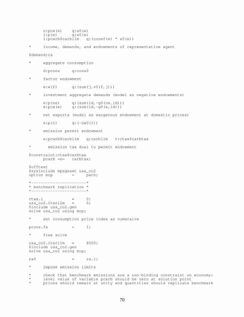
70

o:pce(e) q:a0(e) i:p(e) q:a0(e) i:pcarb$carblim q:(ccoef(e) * a0(e)) * income, demands, and endowments of representative agent $demand:ra * aggregate consumption d:pcons q:cons0 * factor endowment e:w(f) q:(sum(j,v0(f,j))) * investment aggregate demands (model as negative endowments) e:p(ne) q:(sum(id,-g0(ne,id))) e:pce(e) q:(sum(id,-g0(e,id))) * net exports (model as exogenous endowment at domestic prices) e:p(i) q:(-nx0(i)) * emission permit endowment e:pcarb$carblim q:carblim r:ctax$carbtax * emission tax dual to permit endowment $constraint:ctax$carbtax pcarb =e= carbtax; $offtext $sysinclude mpsgeset usa_co2 option mcp = path; *-----------------------* * benchmark replication * *-----------------------* ctax.l = 0; usa_co2.iterlim = 0; $include usa_co2.gen solve usa_co2 using mcp; * set consumption price index as numeraire pcons.fx = 1; * free solve usa_co2.iterlim = 8000; $include usa_co2.gen solve usa_co2 using mcp; ra0 = ra.l; * impose emission limits * check that benchmark emissions are a non-binding constraint on economy: * level value of variable pcarb should be zero at solution point * prices should remain at unity and quantities should replicate benchmark

71

carblim = carblim0; pcarb.l = 1; $include usa_co2.gen solve usa_co2 using mcp; * now suppress listing to save memory $offlisting $offsymxref offsymlist options limrow = 0 limcol = 0 solprint = off sysout = off ; *-----------------* * policy analysis * *-----------------* sets iter iteration over level of carbon constraint /iter1 * iter5/ ; parameters results array for reporting aggregate results p_impacts price impacts (percent change) q_impacts quantity impacts (percent change) c_impacts consumption impacts (percent change) coal_impacts coal input impacts by sector (percent change) oil_impacts oil input impacts by sector (percent change) gas_impacts gas input impacts by sector (percent change) elec_impacts electricity input impacts by sector (percent change) emiss sectoral co2 emissions (mt) mac sectoral marginal abatement cost curves ; loop(iter, * perform benchmark solve first before computing distorted equilibrium carblim = carblim0; carbtax = 0; $include usa_co2.gen solve usa_co2 using mcp; * policy solves with carbon taxes at $50/ton increments carbtax = 50 * co2_carb * (ord(iter) - 1); carblim$carbtax = 1; $include usa_co2.gen solve usa_co2 using mcp; results(iter,"pcarb") = pcarb.l / co2_carb; results(iter,"emissions") = 1e4 *(carblim * ctax.l +

carblim0$(carbtax = 0)); results(iter,"abatement") = 1e4 * carblim0 -

results(iter,"emissions"); results(iter,"cons") = ra.l / 100;

72

results(iter,"% ev") = (ra.l / ra0 - 1) * 100; results(iter,"gdp") = (ra.l + sum(id, sum(ne, p.l(ne) *

g0(ne,id)) + sum(e, pce.l(e) * g0(e,id))) + sum(i, p.l(i) * nx0(i))) / 100;

results(iter,"% gdp") = ((ra.l + sum(id, sum(ne, p.l(ne) * g0(ne,id)) + sum(e, pce.l(e) * g0(e,id))) + sum(i, p.l(i) * nx0(i))) /

(ra.l + sum(id, sum(ne, g0(ne,id)) + sum(e, g0(e,id))) + sum(i, nx0(i))) - 1) * 100;

p_impacts(iter,"pcarb") = results(iter,"pcarb"); p_impacts(iter,ne) = (p.l(ne) - 1) * 100; p_impacts(iter,e) = (pce.l(e) - 1) * 100; q_impacts(iter,"pcarb") = results(iter,"pcarb"); q_impacts(iter,i) = (qd.l(i) / y0(i) - 1) * 100; c_impacts(iter,"pcarb") = results(iter,"pcarb"); c_impacts(iter,ne) = (necons.l(ne) / sum(cd,g0(ne,cd)) - 1) *

100; c_impacts(iter,e) = (econs.l(e) / sum(cd,g0(e,cd)) - 1) * 100; coal_impacts(iter,"pcarb") = results(iter,"pcarb"); coal_impacts(iter,i)$x0("col",i) = (qeint.l("col",i) /

x0("col",i) - 1) * 100; oil_impacts(iter,"pcarb") = results(iter,"pcarb"); oil_impacts(iter,i)$x0("oil",i) = (qeint.l("oil",i) /

x0("oil",i) - 1) * 100; gas_impacts(iter,"pcarb") = results(iter,"pcarb"); gas_impacts(iter,i)$x0("gas",i) = (qeint.l("gas",i) /

x0("gas",i) - 1) * 100; elec_impacts(iter,"pcarb") = results(iter,"pcarb"); elec_impacts(iter,i)$x0("ele",i) = (qeint.l("ele",i) /

x0("ele",i) - 1) * 100; emiss(iter,"pcarb") = results(iter,"pcarb"); emiss(iter,i) = 1e4 * sum(e,ccoef(e) * qeint.l(e,i)); emiss(iter,"hhold") = 1e4 * sum(e,ccoef(e) * econs.l(e)); mac(iter,"pcarb") = results(iter,"pcarb"); mac(iter,i) = 1e4 * sum(e,ccoef(e) * (x0(e,i) -

qeint.l(e,i))); mac(iter,"hhold") = 1e4 * sum(e,ccoef(e) * (sum(cd,g0(e,cd)) -

econs.l(e))); ); file usa_co2_results; put usa_co2_results; usa_co2_results.pc = 6; usa_co2_results.pw = 3000; $libinclude gams2tbl results $libinclude gams2tbl p_impacts $libinclude gams2tbl q_impacts $libinclude gams2tbl c_impacts $libinclude gams2tbl coal_impacts $libinclude gams2tbl oil_impacts $libinclude gams2tbl gas_impacts $libinclude gams2tbl elec_impacts $libinclude gams2tbl emiss

73

$libinclude gams2tbl mac putclose usa_co2_results;