Bulletin Number 86-1

ECONOMIC DEVELOPMENT CENTER

\ •z -I,,- k•• 7•. .."-.

A COMPUTABLE GENERAL EQUILIBRIUM MODELFOR DEVELOPMENT POLICY ANALYSIS

A. Erinc Yeldan

ECONOMIC DEVELOPMENT CENTER

Department of Economics, Minneapolis

Department of Agricultural and Applied Economics, St. Paul

UNIVERSITY OF MINNESOTA

I - -

I

March, 1986

A COMPUTABILE GENERAL EQUILIBRIUM MODEL

FOR DEVELOPMENT POLICY ANALYSIS

A. Erinc Yeldan

February, 1986

Graduate student and Research Assistant, Department ofAgricultural and Applied Economics, University of Minnesota.

Research for this paper has been supported in part by a grantfrom The Cargill Foundation and the International EconomicsDivision of ERS. An earlier version of the paper was presentedas a seminar at the Agricultural Development workshop,University of Minnesota.

I am grateful to Professors Edward Schuh, Terry Roe,%James Houck, and the participants of the AgriculturalDevelopment Workshop for valuable comments and suggestions.All the remaining errors, however, are solely mine.

A COMPUTABLE GENERAL EQUILIBRIUM MODELFOR DEVELOPMENT POLICY ANALYSIS

The purpose of this paper is to present an example of the

so-called Computable General Equilibrium (CGE) models which were

introduced into the Applied Economics literature just a little

more than a decade ago and proved to be very useful for both

medium/long-term planning and development policy analysis

exercises. The underlying motivation for such modelling has

ari sen in r-esp-onse to the well.-known short-comings and

limitations of the partial equilibrium constructs.

Due to the complexities and the interwoven structure of the

real world economies, applied policy analysts have always been

skeptical about the anaLlytical powers of partial equilibrium

models. Thus, the growing need for increasingly general models

has led to the explicit aim of converting the Walrasian general

equi librium system from an abstract mathematical apparatus (as

was formalized by Kenneth Arrow, Gerard Debreu and others in the

195)0s) into a realistic and applicable model of actual

economi es.

The CGE Mode:l.s have, until now, been successfully applied to

many countries, addressing different policy questions.- : L To

cite some examples, the existing models include, but not limited

to: Taylor & Black (1974, Chile) ; Adelman & Robinson (1978, S.

Korea); Dervis & Robinson (1978, Turkey); Ahluwalia & Lysy (1979,

Malaysia) ; Cardoso & Taylor (1979, Brazil); de Melo (1980, Sri

Lanka). Feltenstein (1980, Argentina). de Melo & Robinson (1980,

Colombia), Lewis & Urata (1983, Turkey) ; Lundborg (1984,

Malaysia); Gupta & Togan (1984, India, Kenya and Turkey).

The paper first introduces the broad class of general

equilibrium, macro models that are antecedent to the contemporary

CGE formulations. There, I try to provide an interpretative

essay on such early multi-sector constructs and follow the path

to the evolution of the idea of building price-endogenous, non-

linear macro models that can capture both the market-optimization

behavior of individual agents and the commanding nature of the

exogenously specified government policies.

The second and third sections in turn, build the different

segments of the CGE model. The paper concludes with a compact

presentation of the core CGE equations and two Appendices, one

on the Linear Expenditure System: and another on the endogenous

derivation of the price elasticity of demand, both of which will

be used in the modelling process.

1. INTRODUCTION: A PRELUDE TO THE CGE MODELS

The earliest multisector planning models were based on the

simple input-output linkages among various sectors of the

economy. With these models, assuming a fixed-cofficients --

Leontieff -- Technology for each sector, and given the estimates of

input-output coefficients across sectors, the planner was in a

position to calculate the necessary output level at each sector

in order to satisfy a targeted final consumption bundle.

To be more concise, letting A be the matrix of fixed

input-output coefficients as.ij, with a±j being the amount of

input i necessary to produce 1 unit of opuput j; and denoting

gross output vector by X, and the final consumption vector by C,

the material-balance equation can be written as:

X AX + C (I-1)

Now, suppose- the planner has some targeted consumption

bundle, indicated by the vector C 'Then the "solution" to the

problem can be found by solving the material-balance equation

for X:

X = (I - A) . C (1-2)

Equation (1-2) gives gross production requirements i.n order to

satisfy the targeted consumption demand.

Leaving aside the rather simplistic and cumbersome nature of

the static, fixed i n put-"out p ut model .i ng, thIe most. i mportan t

drawback of such models has been the lack of an optimization

criteria for setting the targeted consumpti-on bundle, C. Yet, in

the absence of such criteria, the determination of C, and hence

of the gross output vector X, becomes an ad hoc exercise in

matrix algebra.

Later, another class of multisector models, known as Linear

F'rogr-ammin ig Models succeeded in overcoming th i s, and many other

shortcomings of the early input-output exercises. cr Here an

explicit objective function was introduced and the problem

involved optimizing this function subject to certain (linear)

constraints. Again, retaining the same notation for X and A, the

static linear programming model can be formulated as follows:

Max RX s.t. Ax :i: B

X U:: 0

where R is a vector of objective function weights and B is a

vector of resource constraints. Given data on R, A and B, if the

feasible set F = {XIAX :i B; X : 0 is bounded and non-empty, then

a solution vector X* can be found to the above problem. <""

Linear Programming Models coupled with the so-called Duality

Theorems have provided interesting implications for economic

problems. In particular, given the above linear programming

problem (primal), the dual problem could be written as:

Min WB s.t. WA R

W C)

where W is a vector of constants. Now, the Duality Theorem

states that a feasible vector, X*, for the primal problem is

optimal if and only if a feasible vector W exists for the dual

problem; such that,

W* AX*--B) = 0 (I-3)

(WA - R) X* = 0 (I-4')

Equations (1-3) and (1-4) together constitute the

complementary slackness conditions. Decomposing (1-3) and (1-4)

we can get the following relations:

W', > 0 implies Ea.i X'* - BE = O (1-5)j

La)jX"j - Bj > 0 implies W* = 0 (I-6)j

X " > 0 implies EW'*aAj - Rj == 0 (I-7)i

EW"ia,..a - R > 0 implies X~* C= 0 (I-8)i

Thus, in general if, at optimum, any one of the constraints

4

in either problems is not binding (i.e. is either strictly

negative or strictly positive) then the corresponding dual

variable carries a zero value,

To carry the analysis a little further, if we interpret the

B vector as fixed supplies of inputs, the R vector as objective

function weights, and the elements of matrix. A as input

requirements of per unit output levels, the complementary

slackness conditions naturally allows us to interpret the dual

multipliers, vector W, as "input prices". In this context,

equations (I-5) and (1-6) state that only fully used inputs have

positive prices and for those inputs where the fi:xed supply

ex.ceeds demand, the associated price must be zero. Further, (1-

7) and (1-8) state that only those activities which do not incur

any losses at the optimum must actually be carried out at

positive levels.

Thus, the linear programming approach provides interesting

insights for the general equi librium relationships of the

modelled economies. However, the fact that the dual multipliers

share the marginality conditions of market prices at the opt:i.mum,

should not be taken to imply that they share other properties of

market prices as well. First of all, such models are based on

the heuristic assumption that a fictitious planner, in command of

all physical productive activities of the economy, yet subject to

certain technological and natural constraints, seeks to maximize

a wellI-defined welfare function for the whole society. They are,

thus, ..Cit. well-suited, nor designed f or the state-capital i st

mixed economies where individual agents independently try to

max:imize their own well-being subject to a budget constraint in

an environment regulated by the government bureaucracy at varying

degrees. In this environment, individual agents taken together

determine certain outcomes that can be affected only indirectly

by the planner. The planner does not have real command on all

the productive activities of the economy, but relies on the

decisions of many other independent "optimizers", each exerting

an influence on the specific development path of the economy.

The remedy to this observation is, of course, to construct a

model where endogenous prices and quantities are allowed to

transmit market information through different sectors of the

economy, thereby simulating the workings of a perhaps regulated

and intervened, yet absolutely decentralized (i.e. not commanded

by a social planner) markets. Yet, this -level of price

endogeneity cannot be designed within the realm of the linear

programming models. To cite the main problem, "the crucial

difficulty lies in the fact that economic behavior and relations

such as budget constraints, consumption functions, and saving

functions must be expressed in current endogenous factor and

commodity prices. But the standard primal constraint equations

of a linear program cannot include th'e "shadow" prices that

result as a by-product of the maximization. Or, to put it

differently, one cannot in general expect that the resource

allocation and production structure determined by the solution of

a linear program is consistent with the incomes and budgets that

result from its dual solution. Indeed, if factor prices have any

impact on the structure of demand, the quantities supplied that

are the outcome of the primal solution will in general not equal

6

the quant.tites demanded that are implied by the dual

sol ut i on 1 ". •

In general, those models which enable this price endogeneity on

the one hand, and incorporate the fundiamental general equii brium

linkages between the incomes of various worker--consumer groups and

the resulting patterns of demand on the other, are termed Computable

General Equilibrium (CGE) models. This paper is about one su.ch

model that inc:orp'orates the :international economy as well as the

domestic markets into the analysis. Given an arbitrary set of

prices, the model solves for the output levels across sectors and

finds the market clearing wage/rental rates. These in turn

become te so:urces o)f income generation for various household

groups and determine the pattern of demand. OQuantities imported

and exported are solved as a function of domestic production

costs, international prices and relevant elasticities. The

investment behavior is also endogenized through the saving

patterns and sectoral investment share parameters, which, in turn

are determined as a function of differential profit rates across

sectors. After calculating excess demands in this manner, the

model updates the initial guess of do.mestic prices through a

Walrasian tatonnement algorithm and iterates the whole process

until convergence is achieved.

It should be noted, however, that the model designed in this

paper can only solve for the relative prices and the

real..L variables of the economy. Yet to achieve this, the planner

has to feed a normalization rule into the model, a completely

exogenous practice. The rule most commonly resorted to and which

will also be used here is to employ a no-inflation benchmark by

defining a constant level of the price index, which is set

exogenously by the modeller. This choice is quite consistent

with the early treatment of Walrasian General Equilibrium Models,

in which only relative prices and real variables would matter,

without much concern devoted to monetary problems. Thus, using

such a normalization rule precludes the treatment of monetary

phenomena as well as the possibility of using such models for

very short-run, stabilization analyses.

On the one hand, incorporation of the interactions between

the real and monetary spheres of the economy in a general

equilibrium framework is still a very difficult branch of

economic theory; and building an ad hoc macro-monetary

superstructure interwoven with the microeconomic general

equilibrium system through simple behavioral equations will have

its own drawbacks as an analytical tool. Further, such

an exercise may turn out to be too general and cumbersome to be a

useful model for focusing on a vast array of development issues.

These arguments should not be taken, however, to imply that

planning monetary phenomena is not possible or ill-advised all

together. Depending on the question in hand and the time horizon to be

analyzed, the monetary sphere of the economy can be incorporated

into the CGE framework in various ways. For example, a very

elegant model that tackled this task quite effectively is provided

by Adelman and Robinson in their 1978 work, which focuses on the

income distribution consequences of different development

strategies in South Korea.

Thus, to recapilulate, the reader has to appreciate the fact

8

that in applied policy analyses much depends on the specific

purpose of the model-building effort and the access to realistic

data supplies, which is still a major restraint on students of

Development Economi cs.

The Model constructed in this paper is adapted and updated

from the works of Dervis et. al. (1982); Dervis and Robinson

(1978); Lewis and Urata (1983); Adelman and Robinson (1978) and

Lundborg (1984). Its distinguishing features are: (1) expliicit

specification of the public enterprises as distinct from private

enterprises; (2) recognition of monopoly power in certain

product markets; (3) recognition of inter-sectoral wage

differences for the same type of labor; and (4) endogenous

calculation of the sectoral expor't subsidies arising from export-

incentive-pack:ages granted by the government.

The Model is constructed and designed to be run in two

stages. The first stage is a within-period general equilibrium

construction which is static in its equations and variables.

Given certain exogenous government policy variables and other

parameters, the Stage 1 Model, as will be called hereafter, finds

the relative prices and solves for all real/structural variables

of the economy. In other words, it comprises the core system of

the overall Model.

The second stage, on the other hand, is designed to up-date

the exogenous variables of the first stage. It is a dynamic

system and basically used for the purpose of "aging" the Model.

Armed with this background we can begin constructing our

model. I first introduce the system of ncotation that will be

9

used throughout the entire Model. Unless otherwise specified, I

adhered to the following legend of principles:

(1) Endogenous variables are denoted by capital letters without

any bar (-) on them. All capital letters with a bar, and

lower case letters (with the exception of d. and rm) are

exogenous variables or fixed parameters in the Stage 1

Model which needs to be updated in the second stage.

(2) All Greek letters are parameters not variables.

(3) Letters with a circumflex (..) are policy variables to be set

exogenously by the government.

(4) Time subscripts are omitted for all variables unless there

are time lags involved. Thus, unless otherwise specified

explicitly, all variables refer to the current period.

(5) The subscripts i and j are used for sectors. They always

range from 1 to n. When these two are used together

(e.g. a:j, or bj.), the first subscript always refers to the

sector of origin and the second to the sector of

destination.

(6) The subscript s refers to different skill types of labor and

ranges from 1 to m.

(7) Subscript f is used to distinguish between the private and

the public firm (p: private; g: public).

10

II - THE OPEN CGE MODEL: STAGE 1

The core equations of the Stage 1 Model in their expilicit

functional forms are constructed in this section. We first begin

with the presentation of the price system.

PR ICES

The specification of the price system in an open economy

model presents some interesting problems to the applied model

builder. To begin with, in the absence of any trade

restrictions, invokiing the neo-classical assumptions, that the

tradables are perfect substitutes and that the country being

modelled is too small to affect the world prices, implies that

the domestic relative prices are set by the given world price

ratios. Thus, there remains no independent, or endogenous, price

system for the model to solve at all. The prices for the open

economy model are determined in the international markets and

these should be fed into the model as given, fixed variables.

However, in practice, especially when we are trying to build

models with limited degrees of disaggregation of the productive

sectors, the perfect substitubility assumption greatly

exaggerates the role of the international price system and the

domestic trade policy over determination of the domestic price

system. The applied macro models, due to the understable reasons

of computation, data limitations, etc., involve a fair amount of

aggregation of sectoral activities, and at such levels of

aggregation the perfect substitubility assumption may lead to

quite misleading results.

Another difficulty, as illustrated by Dervis et. al. ( 1982,

11

Chapter 3) is that assuming the above mentioned neo-classical

hypotheses along with the specification of the productive

technology as one of constant returns to scale, result in

extreme specialization in the sectors that the domestic economy

has comparative advantage, with no home production ever on the

sectors that it doesn't have. Obviously, this is a very crude

portrayal of the way economies engage into international trad.e

and is not supported by empirical evidence. Two-way sectoral

trade is abound, especially at high levels of aggregation.

A formulation to handle these problems has been proposed in

a 1969 paper by Armington which distinguishes commodities not

only by their kind - e.g. machinery,chemical - but also by their

place of production. In Armington's commodity system, not only

is each good different from any other good, but also each

good is assumed to be differentiated by the country of origin

of supply.

Following Armington's hypothesis, domestically produced

goods and imports are assumed to be imperfect substitutes. To

reflect this, we define a tradable composite commodity CCI, which

is a CES aggregation of the domestic commodity DC:t, and the

imported foreign good, M±. The elasticity of substitution of the

CES function, ai, reflects the differences between the domestic

and imported good from the buyer's viewpoint (the smaller the as ,

the greater the difference between DC± and M1 and the harder to

substitute them with each other). Plausibly in sectors such as

agriculture, food processing or textiles, aC is fairly large,

whereas for 'the capital goods sectors it is quite low.

12

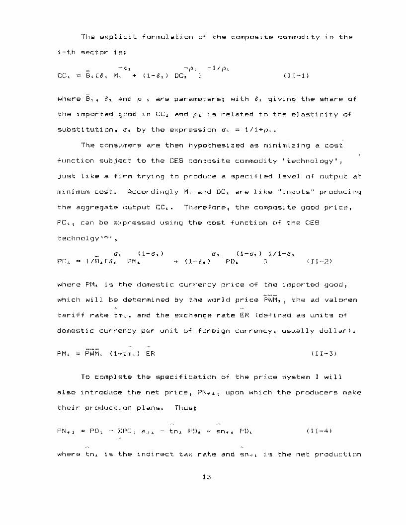
The ex.plicit .formulation of the composite commodity in the

i-th sector is:

--- ":i. -P -I/P/ (CC: = B I. M,. + ( -8,.) DC (II- )

where BS , S. and p . are parameters; with S G giving the share of

the imported good in CCI and p:.i is related to the elasticity of

substitution, o• by the expression ao = 1 /+pi.

The consumers are then hypothesized as mi.nimizing a co(st

function subject to the CES composite commodity "technoology"

just like a firm trying to produce a specified level of output at

mini mum cost. Accordingly M 1 and DC,. are like "inputs" producing

the aggregate output CC±.. "Therefore, the composite good price,

PC-., can be exipressed u.sing the cost function of the CES

te I: hnol. gy < >

ff± ( i-C :k) Cy±. ( l-cr,.) 1 I--PC . = 1 / B . PM . + (1 - 6 ) F D,. 1 ( I :-2)

where PM.i is the domestic c.urrency price of the imported good,

wh:i ch will be determined by the world price F'WM:., the ad valorem

tariff rate tm±., and the ex-change rate ER (defined as units of

domestic currency per unit of foreign currency, usually dollar).

FPM : = PFWM (1+tm,.) ER (I I-3)

To complete the specification of the price system I will

also introduce the net price, PN-=., upon which the producers make

their- product ti on pl an s. Thus;

P N.:i = PD. "- EPCj ac1 - tn. PD,. + sn-c PDF). (11 -4)

where tni is the indirect tax rate and sn.i: is the net production

subsidy. Depending on the government's attitude towards private

versus public enterprises, the granted subsidy rate is

differentiated among firms as well as across sectors. Further,

aji stands for the amount of intermediate input j used for the

production of one unit of i. Hence EPCjaj. gives the value ofJ-t

intermediate inputs used in the production of one unit of the

i-th good.

The two other prices used in the Model, the price of

capital, PKý and the export price, PWEI will be introduced below,

at a later point of the Stage 1 Model. At this juncture,

however, I will turn to the specification of the production

technology of the economy.

PRODUCTION TECHNOLOGY AND FACTOR MARKETS

The crucial assumption in constructing the productive sphere

of the Open CGE Model is that each sector is envisaged to produce

a single commodity (may be thought as an aggregate-commodity in

the Hicksian sense). Conversely, each such commodity is

associated with a single production sector of the economy. This

specification, very much in the tradition of early economy-wide

models, enables us to continue to define the productive sectors

as entries of an input-output table.

As hinted in the net-price equation (II-4), the intermediate

input demands has been assumed to constitute a linear system with

fixed-coefficient production technology for such input-usage..

The retention of this specification is not necessary for the non-

linear CGE Model and extensions of this technology have been

14

t ried in Lewis and Urata (1983) and also in Ahluwalia and Lysy

(1979). For purposes of realism we may need to separate

the technol]ogy of intermediate inputs from the production

technol.ogy for primary inp.uts - capital and labor, Our

specification is perhaps the simplest way to achieve this.

In particular, the production technology available to a

firm can be thought to be given by either a one- or a two-]evel

Cobb-.Dougl as funrction of capital and labor in each sector i,

( -^"f:

:I .rl) L + : -a

X.f±i = A.r K.i Tr LI.U ± (11-5)

or

X f'-. = A i Kf L. I.... .~ . ( II-6)

where L.: is further formulated as a CES aggregation of

di ff:erent skill levels (11-7 below).

The modeller can choo)se either of the spec if icat ion for the

produc.tion technology for a particular firm or sector, However,

the two,-level Cobb-Douglas technology seems to be more realistiic

because it is very unlikely that the elasticity of substitution

between all types of labor is the same and equal to that between

labor types on the one hand, and to capital on the other, as was

assumed in formulation (II-5).

Then, I will retain the two-level Cobb-Douglas technology

for the Model. For such technology, capital is thought as a

f i. xed-coeff i ci ents, composite good with elements b.j• , where b.i j

i s the amount of c api tal good originating from sector i that will

be used to make up one unit of real capital in sector j.

15

Further, capital stock is assumed to be fixed in the within-

period modelling of the first stage. This assumption tries to

capture the fact that capital is not "malleable", i.e. that

combine machines once installed cannot be converted into trucks

easily.

The labor parameter, Li±, of the Cobb-Douglas production

technology is given by a further CES aggregation of m different

skill types. Thus;

I,, . = L- .i (L- ,... , L. i m) ( II-7)

»'n

where L.F:R.o- " R-, is a CES function of skill categories. So we

distinguish between m skill levels in the Model.

More detailed specifications of the production technology

are of course possible. However, more detailed specifications of

the production functions mean more parameters that need to be

estimated, and the applied modeller always faces the trade off

between vigorous functional specification and parameter

estimation. The CES and two-level Cobb-Douglas functional forms

used here require a "moderate" degree of parameter estimation

and have, reportedly yielded quite realistic results in real

world applications (see References).

Now, to turn to the mathematical properties of the

production technology of our model, we should first distinguish

between the gross production possibility set Xf = {Xf ,.. ,X, n

from the nDt. production possibility set, which is:

II N N

X÷ . ",CX . :i. I X . -- X:. a- Eaj X €.:.}4

16

N

The desirab.le property. of course is that the set X.- be

strictly convex. A thnd this is ac hieved i f t he set X + is stri c•tl y

convex and the Hawk ns--Si mon cond i t i ons are sat i s i ed. ) We

basically achieve convexity by assuming capital stocks to be

fix ed. Further, the degree of conve:xity is to be increased with

the number of fix.ed factors of production in each firm, since

this implies the well-celebrated hypothesis of: diminishing

returns to scale to the variable factors.

In contrast to retaining the neo-classical properties in its

productio.n technology, the Model recognizes two ki:nds of

imperfections for the portrayal of market behavior. The first

one is the ex.plicit allowance of monopoly power in certain

productiv e sectors; the other is the recognition of intersectoral

wage differences for the same category of labor.

Incorporation of mono(poly power into CGE type policy models

has not been a common practice (with the e.xception of Adelman &.

Robinson 1978 study). Yet, in a recent p)aper Per Lundb(:rg

provides evidence from the Malaysian tin market showing that the

frequent procedur-e of assuming comp1etitive markets may lead to

m:isleading results (see Lundborg, 1984). Especial.ly, when

analyzing the distributional effects of different policy

packages, existance of monopoly power may have important

consequences which the competitive markets cannot generate. The

income flows arising from the monopoly profits may be

substantial , and may further result in biased innovations (of the

Binswanger -.. Hayami - Ruttan type) affecting the i ntertemporal

grow':.t h I:)ath ( of the ec on omy. <~

17

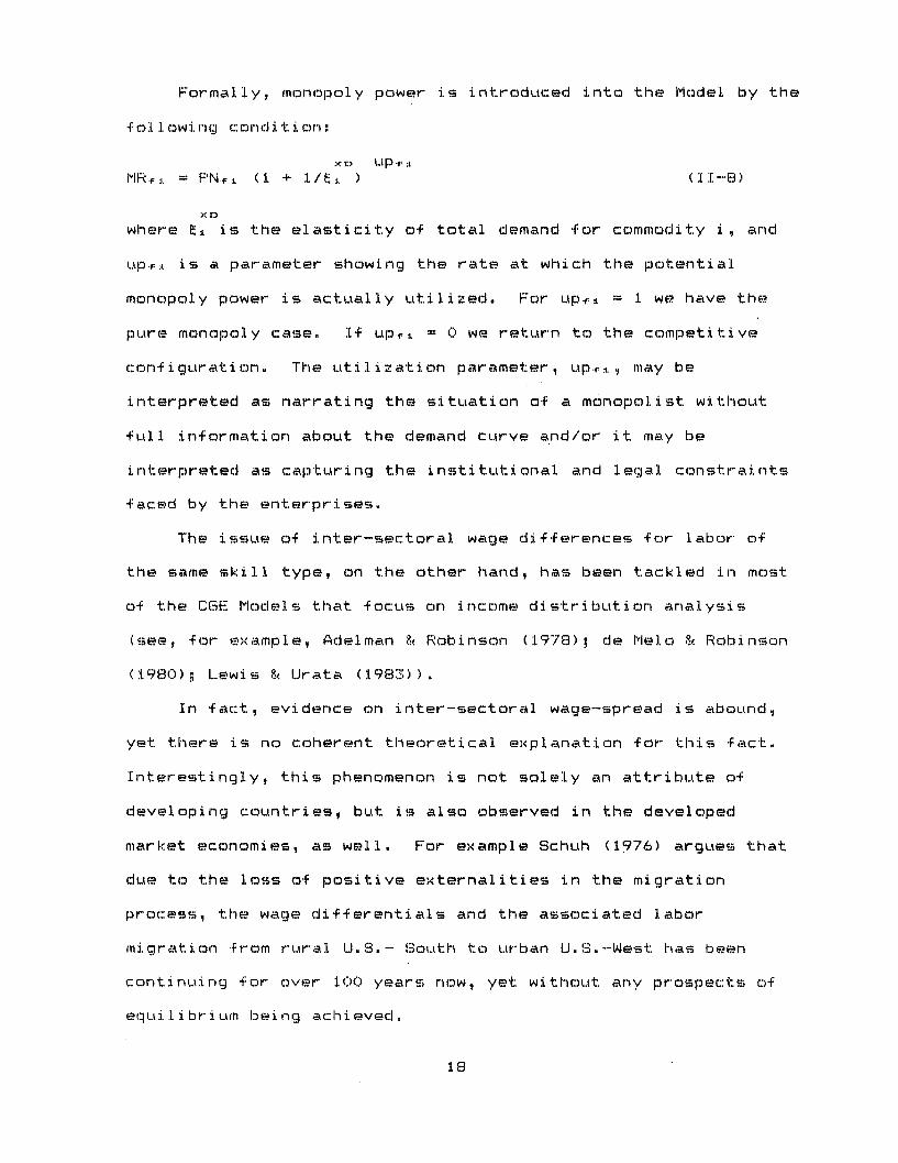
Formally, monopoly power is introduced into the Model by the

foll ow:i ng c:ondition:

xI:) Upp .- :j.

MR.I. - PNN. (i + I1/ .. ) (11-8)

X 0

where .i is the elasticity of total demand for commodity i, and

up.f:. is a parameter showing the rate at which the potential

monopoly power is actually utilized. For up. - 1I we have the

pure monopoly case. If up.f = 0 we return to the competitive

configuration. The utilization parameter, up÷., may be

interpreted as narrating the situation of a monopolist without

full information about the demand curve and/or it may be

interpreted as capturing the institutional and legal constraints

faced by the enterprises.

The issue of inter-sectoral wage differences for labor of

the same skill type, on the other hand, has been tackled in most

of the CGE Models that focus on income distribution analysis

(see, for example, Adelman & Robinson (1978); de Melo &. Robinson

(:980); Lewis & Urata (1983)).

In fact, evidence on inter-sectoral wage-spread is abound,

yet there is no coherent theoretical explanation for this fact.

Interestingly, this phenomenon is not solely an attribute of

developing countries, but is also observed in the developed

market economies, as well. For example Schuh (1976) argues that

due to the loss of positive externalities in the migration

process, the wage differentials and the associated labor

migration from rural U.S.- South to urban U.9S.--West has been

continuing for over 100 years now, yet without any prospects of

eqcuilibrium being achieved.

18

The method -for incorporati .ng wage differentials has

conventi onal ly been to assume cronstants of propor ti onal i ty

between the location of labor and the economy-wide average wage

for that category of labor, which is endogenously determined by

the model to clear the labor markets. Our Model, also, will

retain this method. Thus, denoting the wage rate for labor type

s, employed in sector i, by the firm -f, with Wf:Lt.s; the economy-

wide average wage rate for labor type s by W,,.. and letting the

pr(op:ortionality coef.ficient be \S:&.m we have:

Wfii. 3 = .i1 W. I I-9)

Given the specified production technology and the net prices

from equation (II-4), using (I1-8) and (II-9) one can derive the

enterprise demands for labor of each skill category s. The

private enterprise's demand for labor of the skill type s is

given by the first order conditions of profit maximization:

F'N,::), ± X p, / ....p i. , Wp :, . ( -1 0 )

If one assumes a Cobb-Douglas formulation for the labor

aggregation function in (11--7), using the two level Cobb--.Douglas

technology, equation (II-10-) takes the following form:

L,. = (1/Wp : ) [ ( 1- ) . ),:L 3 MRF:, XSr.:, (I -11)

where >\,,,, is the labor aggregation elasticity with respect to

sl.::ill type s and XS,.. (pr-of it.-max: imizing o.utput.i supply of the

private firm) is given by: (II-12)

19

_-CL. ( -c pL, ) I -3 . .' ) ( -L , ) >p 1 a 1 / Lp, ALX S,:. = A,. Kp,,. MR, N . II ( 1 --a., ) >~:, / Wp 3 3

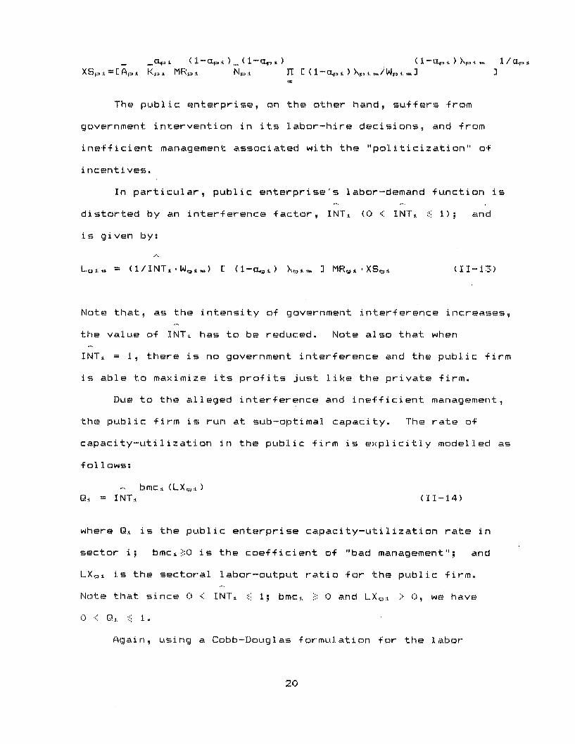
The public: enterprise, on the other hand, suffers from

government intervention in its labor-hire decisions, and from

inefficient management associated with the "politicization" of

incentives.

In particular, public enterprise's labor-demand function is

distorted by an interference factor, INT± (0 < INT' 1); and

is given by:

Lai- . n = (1/INTsWj.) [ (l-(1 . ) >,.i 3 MR, '.XSj.i (II-13)

Note that, as the intensity of government interference increases,

the value of INTL has to be reduced. Note also that when

INTj = 1, there is no government interference and the public firm

is able to maximize its profits just like the private firm.

Due to the alleged interference and inefficient management,

the public firm is run at sub-optimal capacity. The rate of

capacity-utilization in the public firm is explicitly modelled as

follows:

bmc± (LXi )Qi = INT. (11-14)

where Q, is the public enterprise capacity-utilization rate in

sector i; bmc±i:Oi is the coefficient of "bad management"; and

LXi is the sectoral labor-output ratio for the public firm.

Note that since O < INT± :*i I; bmc±i i: 0 and LXi. > 0, we have

0 : Qi :i 1i.

Again, using a Cobb-Douglas formulation for the labor

20

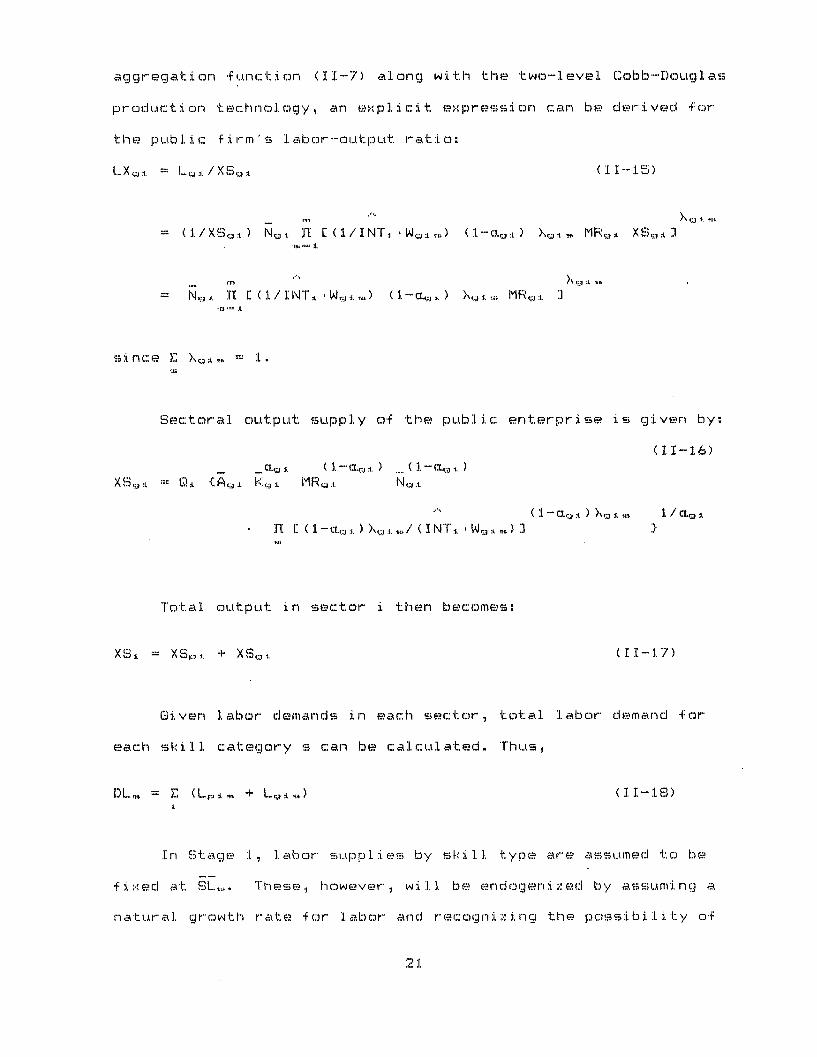
aggregation afunction (11-7) along with the two-level Cobb-Douglas

produc:t:tion te-chnology, an explicit ex.pression can be derived f)or

the pu.bl. ic f i irm's labor -output rat:i. :

LX =,. = L=.. /XS. (I1-15)

rn X. i'

is "um J

rn Xr < I= (IlS,.1 1 ] [ 1 / 1 NT I M Ri, 'WI,.,) >s , .- ,,) i

r s i n c E xsince • c >,j. = i.

Sectoral output supply of the public enterprise is given by:

(11-16)

a_ 0., ( 1 - a., :, ) . ( 1 - a., ± )XS *A, K,: MR ,. N. .i

( 1- .,ýj ) )\3 .1. ,. 1/ (,..kL [ ( 1 -a.c, i. ) -:,.i > / ( I NT'. ' W: : ,.) ]3tun

Total output in sector i then becomes:

XS,. = XS,. + XS, (I -17)

Given labor demands in each sector, total labor demand for

each skill category s can be calculated. Thus,

DL, = E (Lp , + L.i,.) (11-18)i

In Stage I, l.abor supplies by skill type are assumed to be

fixed at SLi,,:. These, however, wi:ll. be endogenized by assuming a

natural growth rate for l.abor and recoglnizing the possibi.lity o.f

21

migratiU.on from agricultural to urban sectors in the second,

dynamic stage of the CGE Model.

Given *fixed labor supplies for each skill category, the

market clearing nominal wage rate, W., can be found via iteration

on

DL S - SL = O (11-19)

Note that, for certain skill categories the nominal wage

rate can be taken as given or having a lower bound, reflecting,

for instance, government's policies on minimum wages. The'n W.fi,

becomes a fixed variable and the level of employment is

determined by the level of demand.

The model can further be enriched by specifying monopolistic

factor markets reflecting labor unions' power and so on. The

flow of the core model, however, will remain the same.

Having derived the wage bill, the profits of the enterprises

can easily be calculated as residuals in the sectoral value added,

Thus, the private enterprise profits become:

RPF' = PF'Nr, XSp:,i - E WpA ,,,:,L LF ) ,,J (II -2"0)

and the public enterprise profits (losses if negative) are:

R C3. PNg± ' XSj. Ez (11-21(II-21)

FOREIGN TRADE

Now we can construc:t the trade equations of our model. On

the import side, recall that we have specifi ed the buyer's

problem as one of cost minimization, where the relevant "cost

function" was one of a CES formulation used to "p3roduce" a

composite commodity, CC., with imported good, M:,. and the

domestic: good, IDC. , taken as "inputs".

In Economics jargon, the buyer's problem is simply to find

the import-domestic demand ratio which satisfies the condition

that the marginal rate of substitution between Mi and DC. be

equal to their respective price ratios.

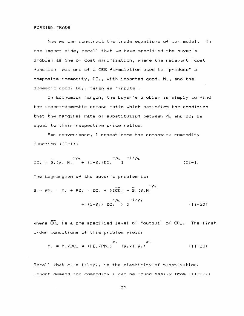
For convenience, I repeat here the composite commodity

function (II -1)

- I. - ::. -"1/p

CCI,. := B.:L .I: M.. + ( - E. ) DC (II - 1)

The Lagrangean of the buyer's problem is:

S = PMi. MI . + PD. * DCi + > LCC B - Bi ( 8M- .

-'.:. - 1 / :'+ (l-&:L) DC± ) ] (11-22)

where CCi is a pre-specified level of "output" of CC:. The first

order conditions of this problem yield:

m i M/./DCt = (PD.i/PM.t ) ( 1/ 1- .. ) (II-23)

Recall that .'i = 1/l+p:.'., is the elasticity of substitution.

Import demand for commodity i can be found easily from (II-23):

Mi. = (PD.i/PMi.) (C/l- . ) DC,. (II-24)

However, at this point DC, is not yet known. It needs to be

calculated and be fed into (II-24). Yet, without knowing the

import-quantities domestic production/consumption decisions

cannot be realized and there is no way of solving for both DC±

and M± simultaneously. A simple trick solves the problem,

however, by using the identity that domestic supply for domestic

market, DS., is given by total domestic supply minus exports. We

get,

DS. = XSi - E, (II-25)

Further, in product market equilibrium we must have

DCs = DSi (11-26)

Hence, using (11-26) we can derive the import demand for

commodity i as:

Mi = (PD' /PMi ) ( /l-i) DS,. (11-27)

which is a workable relation for the Model.

On the export side, we first need to formulate the export

price for each commodity. Similar to the treatment of import

prices as in equation (11-3), the export price relations can be

formulated as follows:

PEj. = PWE± * (1 + SE±.)ER (II--28)

where PEI. is the domestic currency receipts per unit exported

from sector i; SE. is the rate of export subsidy for the product

24

of sector i.; and PWE:,. is the -fixed world price in foreign

C U. r r e n r i ,,

Further, there are certain behavioral constraints that we

have to impose on (11-28) to guarantee meaningful results in the

rest of our model. Note that if PE.,. happens to be greater than

FPD , the domestic price of commodity i, then the Model will

instruct the productive enterprises to export all of the domestic

output leaving nothing for domestic consumption. Such a

situation should, of course exert upward pressure on PD.. until

both prices are equalized. Thus, although there is the logical

possibility that PE:. > PDi. and that all domestic demand for

commodity i mgight b:e satisified through imports, whhil.e all that is

d omest i cal y produced be i n g sol d abroad, we will rule out. t hi s

extreme behavior by recognizing the following constraints on the

ex:port side.

PD. !: PE.i. such that

if PD., - PE. , E !: 0

if PD> PEi , Ei = 0

Yet, another problem is the very hypothesis we have invoked

about the treatment of tradeables in general. Accordingly, we

distinguish products by country of origin and hence, there is the

possibility that the export demand functions .for the home

country's products may be less than infinitely elastic.

The export demand functions for our country's products must

then be in the form:

E. E. (AWPF , PWEI)

where AWPi is an "aggregated" world price for products in the

s ector i 's out!:put category which, as well reflects a wei..ghted.

aver.age of all production costs and trade policies of all

countries.

In designing the specific form of the export demand function

E.( ), we will retain the small country assumption in the

special sense that AWP will be treated as fixed and given.

However, PWE:L now becomes an endogenous price, determined by the

domestic production costs, export policy as reflected in sectoral

subsidy rates and the exchange rate:

PWE, = PD./[ (l+SE. )ER3 (II-29)

From (II-29) we can easily deduce that an increase in our

production costs will increase PDI and raise the price of our

exportables as we present them into the world market. Also an

increase in the export subsidy rate or a devaluation (an increase

of ER) leads to a fall in FWE . In the latter case, if AWF'. were

to remain constant there will be an increase for our country's

export demand for product i and hence, an increase in our world

market share.

Following Dervis and Robinson (1978) and also Dervis et. al.

(1982) one can make the assumption that the world consumers as a

whole behave according to the rules of cost minimization with a

generalized CES function specifying the world commodities as a

composite good. We can then specify the export demand functions

in the single elasticity form:

26

E . = E., (AW ./ PF'WE ) ( I -30)

where ':(. is the elasticity of export demand and EJ.i. is the normal

trend level of the home country exports when AWP:I. PWE,.

Having thus constructed the export demand equations, what is

left for us is to find an endogenous expression for the export

subsidy rate, SE,.. Many governments, instead of granting a

single ad valorem subsidy rate to ex porters, provide a comp:lex

set of incentives for producers to encourage the ex.portation of

their products. These incentives may range from beggar-thy-

neighbor mercantilist policies, to a laissez--faire treatment on•

tradables. In this paper, a policy pacl.kage consisting of four

different ex.port incentive schemes is recognized and explicitly

modelled These are: (1) rebates on pr.).oduction taxes, tn.: , son

the products destined for exports; (2) allowance on the corporate

income tax at a certain percentage rate of export earnings; (3)

permission of .duty free intermediate 'imports used for the

production of exports;. and (4) a sectorally di.fferentiated ad

valorem export subsidy (tax if negative) rate which is directly

paid out of the government budget.

It w:i.ll further be assumed in the Model that the government

sets sectorally differentiated "eligibility criteria" on ex.ports

that may benefit from the above schemes, such as exports destined

for designated world markets, or export earnings exceeding some

minimum value in foreign currency, etc. Depending on the

st. r i ctness of these cond i t i ons it will b e assumed that the

eli gi bility rate for exports in the pr'od.ucti on tax r'ebate and

allowance on corporate income tax schemes is historically around

27

ee. percent of total exports. For the remaining two schemes ee

is taken to be 100.O

Therefore, under the first scheme total subsidy granted to

sector i will be:

TSR± = tn:. * ee:L * FPWE * ER * EE (II-31)

which corresponds to subsidy equivalent of tn. * ee± percent..

Under the corporate income tax allowance scheme, total income tax

allowance granted is:

TKA = kta * Eee * PFWEi * ER , E, (II-32)

where kta is the granted corporate income tax allowance rate.

Letting tk denote the capitalist (corporate) income tax rate,

total subsidy on exports due to this scheme is:

TSA:. = tk kta * eel PWE. * ER * E. (II-33)

which corresponds to an ad valorem subsidy of tk , kta ee.

percent.

As for the third scheme, observe that the domestic currency

value of imported intermediate inputs used for export production

is:

EMI. = EPWMj * ER * dj , mj * a.: E± (II-34)J

where d. is the domestic use ratio of the j-th composite good

(see equation 11-57 below); and mnj is the import-domestic good

ratio introduced in equation II-23 above. Thus d * mj * 'a

gives the amount of imported intermediate good j, per unit of

good i produced and exported.

28

Total import tax to be paid on such imports then becomes:

T"EMI' =T Etmj. , P WM..1 , ER R dj , m.J a...j Ei (II--3 )

which gives rise to an ad valorem subsidy rate of

Etm.j* FWM *dj mj aji * (1/PWE. ) per unit of exports.-i

Combining with an explicit sectoral subsidy/tax rate of te.

on exports, the realized overall export subsidy rate becomes:

SE:i. =- (tn . + tk * kta) ee,. (II-36)

+ Etm.j * PWMI. d.. m .. a.j.2 (I/PWE: ) + te,.J

which appears in PWEi in equation (11-29). Note that since the

above expression further entails PWE. , it needs to be

solved by numerical methods.

Balance of Payments EquIilibrium is then achieved when,

EPWM * M:. - EF'WE:,. E. F- F - WR C 0 (I1-37)± .

where F and WR starnd for the ex:ogenous value of the net foreign

resource inflow and workers' remittances, respectively. If the

exchange rate is allowed to adjust freely (which is as well a

policy decision, hence we continue to use a circumflex. on ER), ER

will need to be iterated until (I1-37) is satisfied. Per contra,

if the government chooses to fix ER at some value, there is no

guarantee that Balance of Payments Equilibrium would be satisfied

(a surprise to no one!); hence, the government would need either

to ration imports or try to increase exports, or get more foreign

resources. Such commercial policy analyses using CGE Models are

abound and the interested reader may wish to consult with the

works cited :i.n the References to this paper.

29

INCOMES GENERATION, CONSUMER DEMANDS AND SAVINGS

The functional incomes of different consumer groups of the

Model are generated using the results derived in the factor

markets and the derivations are quite straight forward.

For labor- skill-type s, assuming that the tax rate is ts

total disposable income can be written as:

YL. = (1-ts) E (WI ',Lp,. + W S..Lg.±.) + ) 4 *WR'ER (II-38)

where w is the share of workers' remittances captured by labor

group s.

Capitalists' disposable income becomes:

YK =: (l-tk) ERP, (I 1-39)

Fublic enterprises' aggregate after-tax income is:

YK3 = (1-tk) ERG. (II-40)

Government's total income is:(II-41)

YG = Ets E(WpisLpi, + W,.iL,,,)

+ tk E(RF'. + RG± - kta'eei*PWE. sEREi±)

+ ECtm ,*PWM.t ER,'M-EtmAjPWM., ERd-j *mj a.1 ,E±3

+ Etni :F'PDXSI-ee: '*PWE± 'EREi] - Yte *PFWEi *ER E,. sn

- 1 [sn± ,PD'D. ,XSp,. + sn<.i ,PD± *XSc± ] + YKG + FER

Given total incomes for different socio-economic groups, our

next task then, is to cal culate the components of domestic demand

for each sector.

In the absence of money markets and any specification of

lending behavior, the investment demand is totally savings-

determined. Hence, the savings-pool of the economy sets the

limits of the investment demand, and capital formation in

general. The model distinguishes between private and public

savi ngs/cnsumpt i on behavi or . Private agents are assumed to save

a fraction of their disposable incomes, given corresponding

savings parameters. The government on the other hand, is assumed

to set an exogenous policy on the required public investments as

a proportion of total GDFP and given this exogenous policy ratio,

it withdraws the necessary fraction of its total income as

savings.

In particular, total private savings, TPS is the sum of the

savings of all workers of skill types and capitalists:

TPS = ES, YL.. .. + sk YK (II-42)

where S. and sk are saving rates out of labor income of skill--

type s and capitalist income, respectively.

The government is assumed first to establish a policy on the

ratio of total public investment to gross domestic product.

Denoting this policy ratio by 8, the necessary investment fund

of the government, GIF, can be found:

IF "= 9 ( L-PD: XS.. - YE PC j a. XSi) (II-43)wi ;i. J

where the expression in parantheses gives the nominal gross

domestic product of the economy. Having stated GIF, the required

savings rate for the government is given by:

Sg = GIF/YG (11-44)

Once the saving decisions are made, what is left for the

transactors is to determine the consumption demands for each

product. The private and public consumption functions will again

be distinguished, reflecting the state of affairs that private

consumers' demand functions are derived by way of preference

maximization, but the government's decision are exogenous in

nature. One can, of course, specify a preference map for the

government bureaucrats as well and derive government's demand

functions from that map. This, however, would be a very

complicated task involving heuristic assumptions, and requiring

very specialized data sets which would, most probably, be beyond

reach for most of the developing countries.

The private consumption demand function will be given by a

linear expenditure system (LES) of the following form:

For labor-skill s:

C L. '. t = T.+ / F'P:C ( 1 -S.)YL.-EPC.F j3 (11-45)

where r.i is some absolute minimum (subsistence) level of

consumption of commodity i for group s. The expression in the

parantheses gives the total income in excess of the expenditures

over the subsistence-basket. The parameter ,,,, is the margiDina•l.

budget share of product i, and it tells how consumer group s

allocates its marginal income above the subsistence level across

32

sectors. The derivation of the LES and its properties are

fur ther' e x am i ned i n Appendix. A.

Th e cap : tal. i st consumpt ion demalnds al so f oil lw the same

f or mat,

CK T ,..:. + ,: /F PC:i. : (1-sk) YK - EPC- ,. j (11-46)

The government consumptian demand will be assumed to be of

the following simple form-

CG:,. q:· (1-Sg) YG/PC ( 11-47)

where q. is the policy-induced public expenditure share for the

product of sector i.

The total consumption demand for product i then, can be

found as the sum of private and public consumption demands,

C:1. = L CL,. + CK. + CG.( (11-48)

To construct investment demands, recall that we assume total

investment demand to be constrained by total savings generated in

the economy. The Model determines sectoral private investments

thro..ugh e.xogenous investment allocation coefficients, Hl:.. These

coefficients are then endogenized in the Stage II Model by using

previous period's prices, production costs and pro.fit rates.

Real private investment in sector i is:

NPF. = H:i. ("I"TPS/FPK ) ( 1-49)

where FPK is the price of capital.. Si nce capital is a fixed-

coeffic:i. ents composite commodity its price is given by a wei.ghted

33

average of its components:

PK. Eb ..j PCj (I -- 50).J

Real public investment in sector i is found in analogous

manner, yet here sectoral allocation coefficients, HG3, are truly

exogenous (i.e. not endogenized in the Stage 2 Model, but only

up-dated). This treatment reflects government's sectoral

priorities for investment. Thus,

NG. = HG:L (G IF/PK ) (II -51)

total real investment to sector i is then:

NT:L = NPi + NGB: (I1-52)

Now, note that NT± gives the amount of real investment to.

the i-th sector. Yet, for national income accounting purposes we

need to know the amount of investment demand from sector i. In

Planning Literature, the former is referred. as "investment by

sector of destination", and the latter as "investment by sector

of origin".

Therefore, to get real investment demands by sector of

origin, Z., we use the capital composition coefficients once

again and arrive:

Zi = Eb. (N'T.) (II-53)j

The last component of total demand is the demand for

intermediate inputs and can be calculated easily using the input-

output coefficients. Letting Vi denote the amount of

34

intermediate demand from sector i,

V . Eaa . XSJ (I-54)

The total demand for commodity i, TD., is then:

TDi = Cs + Z.L + V:L (II-55)

Now, since we have found the magnitude of total demand f:-)r

each composite p:roduct our final task is to decompose this

magnitude into its two components: domestic and foreign. TDI:. of

equation (II-55) gives total demand -for the overall composite

good, as was defined in (II-I). In the meantime we have derived

domestic output supp:lies and in order to -find the market clearing

domestic prices (PD: 's) we need domestic demands as well.

Important as it is, this is not a complic-ated task, especially

when we use certain mathematical properties of the CES function

which deffines the compos:i.te good in (II-1). It can easily be

shown that the CES function in (II-1) is linearly homogenous in

its variables, Mi and DC:., and can be re-written as:

CC. C = f . (m. ) , I.1) DC.. (1: -56)

where f .1. ) specifies the CES function given in (II-I) We then

have:

d,. = DCI/CC:. = fi (mi,l) (II-57)

Since mi is a function of the relative price ratio PDi./PM.

(see equation II11-23), d is uniquely determined by FPDI:./PFM as

well. It must be noted, however, that the demand for the

composite commodity, CC., depends on all of the relative prices.

We can use di and go from composite commodity demand to the

domestic demand for the domestically produced commodity,

DC. = di * TD: (II-58)

Adding export demand of foreign consumers to domestic

demand, we get the total demand for domestic product i:

XD = DCi + E:L (11-59)

Market-clearing conditions imply that all excess demands be zero,

XD. - XS6. = 0 (I1-60)

The solution strategy of our static CGE Model then starts

with an initial guess of domestic prices, PDi, the wage rates,

W,,,, and the exchange rate ER. We first calculate the excess

labor demand in factor markets and revise wages until these

markets are cleared. Then, using the labor aggregation and

production functions we calculate sectoral output supplies. In

the meantime, from wage and profit incomes, labor and capitalist

incomes are generated; while government's total income is given

by the tax revenues, public enterprises' sectoral profits and net

foreign resource inflows. From incomes generated, savings and

consumption decisions are carried out and the savings-pool is

turned into sectoral investment demands by the sectoral investment-

allocation parameters and capital.--composi ti on coefficients.

Import and export demands are derived as a function of domestic

and world prices, tariff/subsidy rates and the exchange rate.

36

Once product e.cess demands and the Balance of Payments equati on

are d eter m i rn ed, t he i n i t i a l g u ess o f r.:d omesti . c:: pri c:es and the

exchange rate are revised so as to satisfy the condition that

they will be suffici ent y close toW zer(". "' With the new set of

domestic prices and the exchange rate the Model is solved once

again and this process continues until convergence is achieved,

As we have discussed previously, however, we know that the

Model obeys the Wallras' Law that the value cof all ex.cess demands

add up to zero. This means that if I'PD = {PD I , . ... , I'D,·, is a

set of soluti on prices so is t F'PD" for any scalar t>0 ; and it

is the Planner's job to specify a normalization rule to set the

relative price system for the Model. I have adopted a "no--

inflation" procedure and chose to normalize the price system

around a gi ven index P:

EPC. Q• = (II-61)

where S"Qi. are the weights defining the index PF

Equation (-61) closes the system of eati(--) cse te stem tions of Stage 1.

A sketch of an ex.istance proof for the core model is presented in

Dervis et. al . (1982) and the interested reader can get an

intuitive n-otion of the general equilibrium properties of the

Model from the analysis presented there. "iihe stability

properties of the Model are actually implied in the solution

algorithm used for the iteration of prices to clear the excess

demand equations in (II-60). Thus, practically what is left for

us i s to: go on to t he Stage 2 Model and upda'te anid/or" endogen ize

t he e;xogenous variables of the static St.age 1 Model equati ons.

37

III - THE OPEN CGE MODEL: STAGE - 2

As stated earlier, the task of the Stage 2 Model is to up-

date and endogenize the fixed variables of the first stage.

Here, some of the variables may need to be up-dated using certain

regression/trend-line modelling; while certain others may warrant

some behavioral model specification. 9"' For those variables of

the former type, the "aging technique" is left to the planner..

Thlis may be accomplished using simple trend-line equations,

forecasting methods, etc. Adelman and Robinson (1978), for

example, provides an inspiring tabulation of such exercises, and

the interested reader may wish to consult with their methods on

revising the exogenous variables of the Stage 1 Model.

In this section, two variables are selected and modelled

using behavioral equations, just to give an example on such

modelling. The variables are: labor supplies; SL, (equation

reference, 11-19) and private investment allocation parameters,

H1 . (equation reference, 11-49) though, of course, this selection

is by no means decisive for all types of constructs. The

behavioral models are taken from Dervis and Robinson (1978) and

Dervis et. al. (1982). Lewis and Urata (1983), also used them

with some minor changes in their planning exercises on Turkey,

for the period 1978-1990.

LABOR SUPPLIES AND RURAL-URBAN MIGRATION

Labor supplies of different skill categories are endogenized

through exogenously specified natural rates of population growth

and endogenous migration from rural to urban sectors. Assuming

th a t ri..l..:tura 1. ab or is d :i st i ngu shed by ski : 1 type- 1 and

tha t a: l other ski ll types, s=2 ,..., , corr'espond to di4fferent

(categoriet s o f :urban. .abor, we have the fol owin g s ystem o.f :abor

supply equations:

SL. (t+1) = (l+r ) SL.(t) - MIG(t) (III-i)

SL..(t+l) = (l+r ) SL (t) + (SM.) MIG(t) (III-2)

s = 2, ..,m

where 1, (s=,...,m) is the ex.ogenously specified natural .growth

rate of the labor force - type s; SMl. is the share of

agricultural labor that joins the ranks of the urban labor force

type-s (plausibly SM,., will get a smaller numerical value as one

goes higher in the skill levels di st ingui shed for the urban

sector). MIG(t) is the number of agricultural workers leaving

their occupations and joining to the ranks of urban labor force.

Following Harris and Todaro (1970), migrati on is seen as a

f unt ction of the di fferences between the rutral. and expected u.rban

wages. In particular,

MIG(t) = ... L (EW,. - W,.)/W .] SLi (t) (III-3)

where vg is a parameter measuring the responsiveness of migration

to the differential between agricultural and anticipated urban

wages; and EW.... is the expected urban wage, which can be

formulated in the following simple fashion:

EWu .... E E C: Wr.,i.. (t)* L .±, (t) + W•.:i.t„(t) '* .. (t) 3 1/L.. (t)w I-h .L m-t it (I II-4e)

where L,..,(t) is the total urban labor force (note s=,...,m).

39

SECTORAL ALLOCATION OF PRIVATE INVESTMENT

Private investment behavior is one of the hardest aspects of

applied planning exercises. Theoretically, private investment

demand is affected by a whole set of variables, such as expected

sales; past, present and expected future profits; profit rate

differentials across sectors, as well as by the availability of

the investment funds. In the previous applications of CGE

Models, one of the most elaborate formulations of private

investment behavior has been used by Adelman and Robinson (1978).

In their model, investment demand and supply of loanable-funds

decisions are carried out by different sets of agents. Through a

simple model of expectations, enterprises form their investment

demand decisions and demand funds from the loanable-funds market.

Further, supply of funds come from various sources such as

organized banks and the unorganized, curb market.

General and realistic as it is, the data base and effort

required for such a construction is really tremendous and makes

it very difficult to be applicable in development policy

analysis. For this reason, I will resort to a less ambitious

construction, one that has been used and tested successfully in

the applied experiments of Dervis and Robinson (1978) and Lewis

and Urata (1983).

In the Model used here, investment shares are seen as a

function of the relative profit rate of each sector compared to

the average profit rate as a whole. Sectors that have higher

than average profit rates, then capture a larger portion of the

private savings-pool. According to this formulation, investment

40

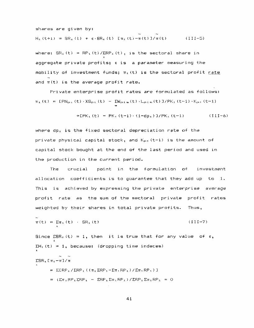
shares are given by:

Hi (t+1) = SR1 . (t) + e SR:. (t) E11.j. (t)-rr(t) :]/IT(t) (III-5)

where: SR. (t) : RF'P: (t)/ERPF' (t) , is the sectoral share ini.

aggregate private profits; e is a parameter measuring the

mobility of investment funds; ir. (t) is the sectoral profit r.ate

and Tr(t) is the average profit rate.

Private enterprise profit rates are formulated as follows:

+':PK. (t) - FPK (t-1) * (l-dp. ) J/PK:. (t-1) ( 111 6)

where dpi. is the fixed sectoral depreciation rate of the

private physical capital stock, and Kp (t-1) is the amount of

capital stock: bought at the end of the last period and used in

the product ion in the current per i od

The crucial point i n the f ormulIat i on of i nvestment

al Iocat i on coef ficients is to guaraantee that they add up to 1.

This is achieved by expressing the private enterprise average

profit rate as the sum of the sectoral private profit rates

weighted by their shares in total private profits. Thus,

Tr(t) = E .(t ) ( SR:. (t) (I I-7)i

Since ESR, (t) = 1, then it is true that for any value of e,

ESRI : TI - T 3/i.

= C RPF,. / ERFP. ( ( rr ERF'P. - ETrr . RPF. ) / Err i RP . ) 3

= ( ETr .. RP ERF' -" ERPF i E'rr :. IRP., ) / ERP :. Err RPi = 0

41

What remains is to up-date the sectoral capital stocks of

the enterprises. Here, for the purposes of realism, one can

specify gestation lags for installation of the capital stocks.

Thus, the capital stock that will be used in the next production

period will be expanded by the investments of the previous years

finished after a certain lagged period of time. Accordingly,

private enterprises' stocks of physical capital which will be

used in the next period's production process will be given by:

Kpi (t)= Kpi (t-1). (-dp.) + E Ap,,±, NF'P (t-r) (III-8)

where Ri,.. is the proportion of capital goods bought in time t-r

that will be installed to the private firm operating in sector

i, by the end of the current period. It must be true that

E pA.r = 1. The variable T is the longest gestation lag,

whereas the minimum lag can be set at one year by letting

p 1. c:> 1.

Public enterprises' physical capital stocks which will be

employed in the next period will likewise be:

T

Kgi (t) gL (t)-l) (1-dgL) + E A ,.r NG. (t-r) (III-9)*r" nm ir.

This completes the construction of our Open CGE Model. In

the next section I present the equations of the Stage 1 Model in

a compact form. The presentation is designed so as to encompass

a variety of applied problems; yet the specific modelling effort

should, of course, always be suited to the special

characteristics of the problem at hand.

42

IV - EQUATIONS AND VARIABLES OF THE OPEN CGE MODEL - STAGE 1

In this sect ion I lay down the core equations of the Stage 1

iMolel. Tab e 1. gives the equation summary on pri ces, Tabl e 2

gives the equati. ons of factor markets and product supplies, and

Table 3 presents those of the product markets.

T'A B I E Pr ices

Composite commodity

CC. = Bi8 C .MS I ( 1-- )DC. 3

No. of....... ..sn..... ...

n

Re erence

(II-1)

Composite good price

I'C C. (/B 1- ~M )PC. = l/B,.c. PMF .

+. ( 1-c ) 1/)- D:,+ ( :L-S ) PD0± ]

Price of the imported good in domestic currency

F'PM:. == 'WM: (l+tm ) ER

Net price or value added (f:=p,g)

1- N- = PF'D - CF'C .a .. - tni.FPD + sn .PD .

n (11-50)Frice of capital

PK± = L Eb ., PC..

Normali zati on

E'PC. * S. = P

Total 4 6n + 1

n (11-2)

n

(I1-4)

(I 1-61),

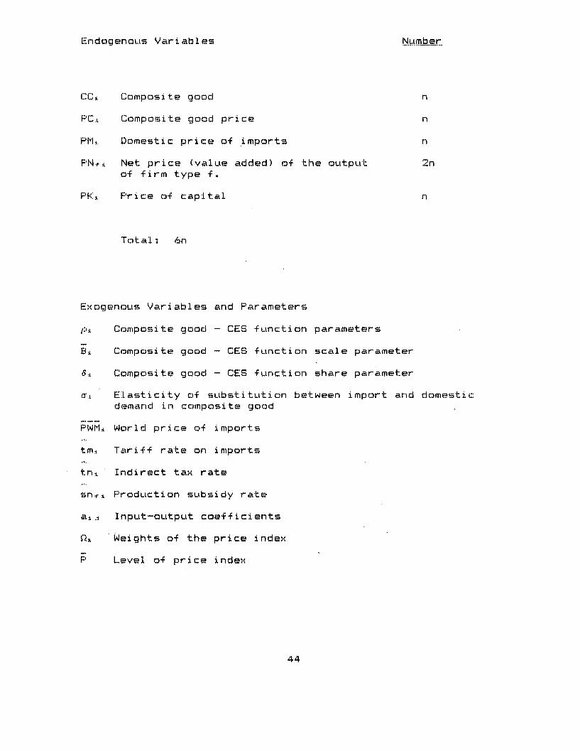
Endogenous Vari ables

CC.,. Composite good n

FPC. Composite good price n

PM:. Domestic price of imports n

PN÷j Net price (value added) of the output 2nof firm type f.

PK± Price of capital n

Tota : 6n

Exogenous Variables and Parameters

p' Composite good - CES function parameters

BE Composite good - CES function scale parameter

6. Composite good - CES function share parameter

a•. Elasticity of substitution between import and domesticdemand in composite good

PWMW World price of imports

tm. Tariff rate on imports

tn. Indirect tax rate

sn.i Production subsidy rate

aij Input-output coefficients

S1 Weights of the price index

P Level of price index

44

N.u.mb.e.r.

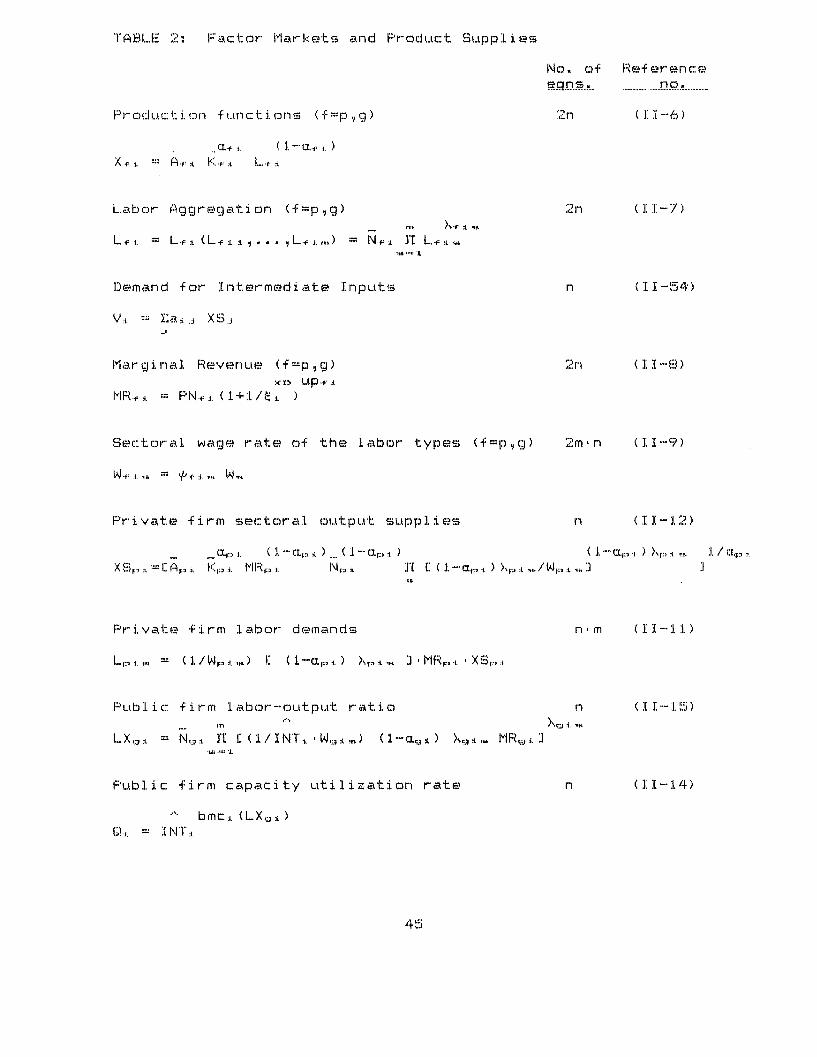
TIAB9LE 2: Factor Mark::ets and Product Supplies

No. of Reference..e ..._...& . s.... ...... ............... .n ... ...........

P r o d uc t i o n f u n c t i. on s ( f = p , g) 2n ( 1 -6)

... .. .: .,. ( 1 - .f :, )X * :,. "::: A ff: . K . L • I.

Labor Aggregation (f=pg) 2n (I1-7)

L es. = L.f A (L.f i..1. L.fi, :. m) = N I i : L..f•r,

Demand for Intermediate Inputs n (11-54)

V:i. = EaT :..j XSj.J

Marginal Revenue (f=p,g) 2n (II-8):;< up-. ..

MR.f . = PN.=,. (1+1/sI )

Sectoral wage rate of the labor types (f p,g) 2mn (1-9)

Pitf. l. efir ctotn ( -9 )

Private firm sectoral output supplies n (II-12)

Sc:. ( 1 - :., * ) ( . - (., .. ) ( 1 ""a.,: ) >,r .. 3 1 / .X S,.,:. . 1: A,.. K::,: .. MR,::, Np, A" [ ( 1 - a.,.:, ) ,:, ... / W,::.> ... . :]

Private firm labor demands

L,. = (1/W i,:, ) I: (1-0.I:,. t) X, p. ± . 1* 'MRM . * XSr,:,.

Public: firm labor-output ratio

LX,• = N,1 II [ (1/INTi N *W,.) (1- l .) >,.:Ls R MR" l

Pub.lic firm capacity utilization rate

bmc. (LX,• )Q:. = NT,

n m (I I- :l 1 )

n (11 -15)XA -j - I.

(11 -14)

45

Public firm sectoral output supplies

XS, .. = s Q). K . MR<i N

(1-H [; ( 1-a-. ) > . /( INTl(i ' W ,) 3

Public firm labor demands

L,:. = (1 /INTi W, ,,) C (1-.,. ) >, . 3 MR, XSJ.

Aggregate Labor Demands

DLM = E (L., + L • )i

Excess Demands for labor

DL_ - SL, = 0

(I1-16)

1 / a, :

ns, )m

n*m ( I I-13)

n (I1-18')

r (I1-19)

Sectoral Profits of the private enterprise

RP F' PFN,.. , XSp, - E Wp. ,L,:,.

Sectoral Profits of the public enterprise

RGi = FPN j.* XSc ,. - Z W,•iý gLc,,

Total sectoral output supply

XS. = XSrS,. + XS S;.

n (11-20)

n (II-21)

n (II-17)

Total: 14n + 2m + 4n m

Endogenous Variables

X.FA Sectoral production technology ofthe firm type f

L. .. Labor used in sectoral production, bythe firm type f

Number

2n

46

n

V Demand for Inter'mediate inputs n

MR. i Marginal Revenue of the firm type f 2n

Wf,-.-m Sectoral wage rate of the labor type s 2n* memployed by the firm type f

LX ,i PFublic firm labor-output ratio n

FQ. Public firm capacity utilization rate n

XS.L:k. Sectoral output of the firm type f 2n

L+.'.I Labor demand by sector and type 2n m

DLV Aggregate labor demand by skill-type m

WI Average nominal wage rate by skil:L type m

R.f . Sectoral profits of enterprises 2n

XS ,. Total sectoral output supply n

Total. 14n + 2m + 4nL* m

Ex::ogenous Variables and Parameters

A-i Production function scale parameter

Kf:,. Sectoral capital stock of the firm type f

(I. .. Product:::tion function share parameter

N.,: : Labor aggregati on . functi on scale paramreter

.,.. Elasticity of labor aggregate in sector i with respect tolabor skill type s, employed in firm type f

SL., Aggregate labor supply by skill type

t. Elasticity of total demand for the domestic product

up.• : Firm type f, monopoly power utili.ation parameter

S.. Coefficient of proportionality of the sectoral wage ratetoc average wage rate of labor type s employed in firm type f

I NT :. Coef f i c:i ent :of g aver nment i ntrf erenc:e to the pu..b: i c i rm

bmc::,. Caoe.f f: i c:ient of "bad man agement " in the publ ic f irm

47

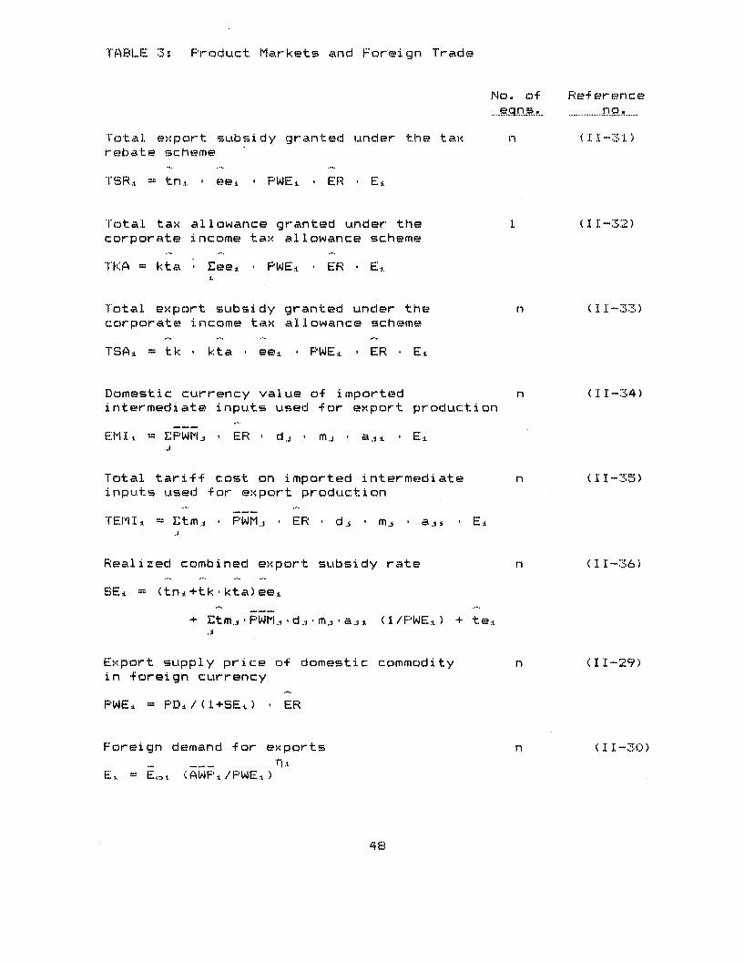
TABL.E 3: Product Markets and Foreign Trade

N

Total export subsidy granted under the taxrebate scheme

TSR. . = tn. * ee * PWEI * ER E.

Total tax allowance granted under thecorporate income tax allowance scheme

TKA = kta ,* ees * PWEP * ER * E.

Total export subsidy granted under thecorporate income tax allowance scheme

TSA, = tk * kta eei , PWE * ER E.

Domestic currency value of importedintermediate inputs used for export production

EM:I. = EPWMj * ER * d. m.j * aj. * E_J

Total tariff cost on imported intermediateinputs used for export production

TEMI" =E tm.j PFWMj * ER d-j mj * a.ji * Ei..j

Realized combined export subsidy rate

SE, = (tni+tk kta)eeL

+ Etmj PWM 4 d, dj ,*m aj i (1/PWE. ) + te.±

Export supply price of domestic commodityin foreign currency

PWE± = P Ds./(1+SEi) , ER

Foreign demand for exports

E. = E= < (AWF'i/PWE..)

o. of

n

Reference....................... .....

( 11-31 )

(II-32)

(I-33)

n ( II-34)

( I1-35)

n (II1-36)

n (I -29)

n

48

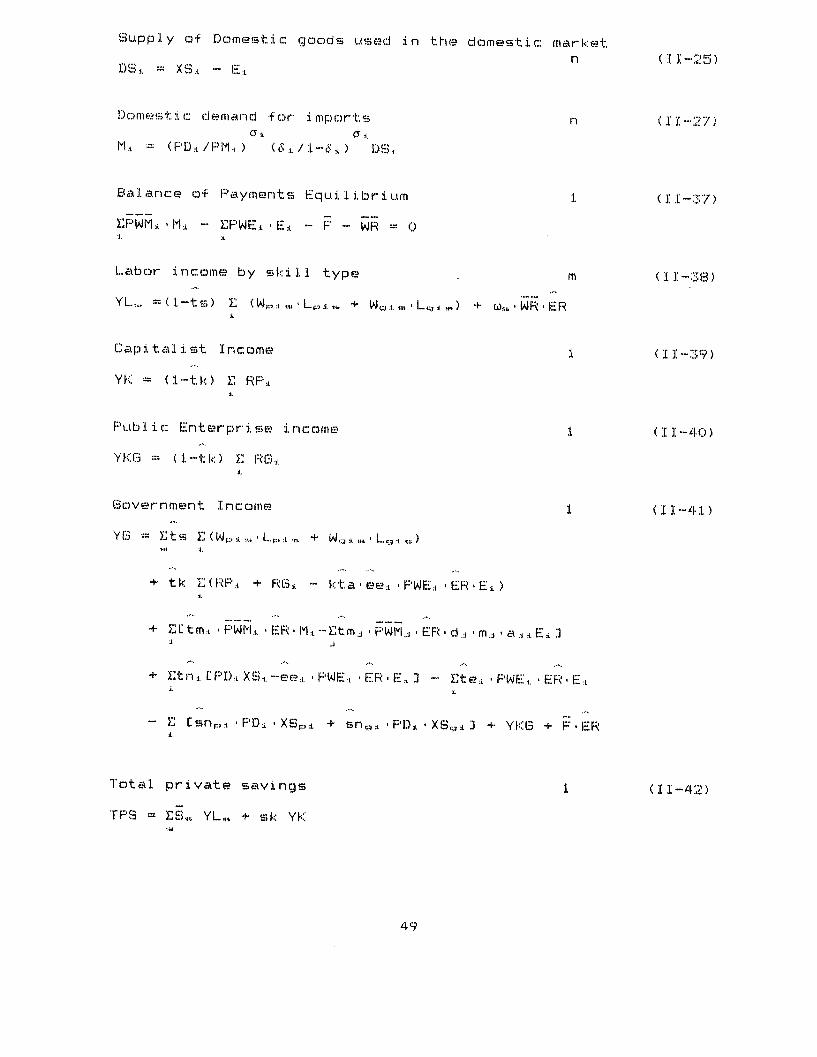
Supply of Domestic goods used in the domestic marketn (II-25)

DS.i. XS.i. - E:i

Domes t i c( d e emand for i mpor ts n (1 -27)(7-i.

M . = (PD. /PM i) ( . / 1 .- 6 ) DS

Balance of Payments Equilibrium (II-37)

EPWM. 'M:I. - EPWE: i'E . - F - WR = 0

Labor income by skill type m (II-8)

YL.,,. =(1-ts) E (SW , .'L,,...i + W,:s.,Lc, ) + w, ,*WRERI.

Capitalist Income (II-39)

YK = (1-tk) E RPF':,.i.

Public Enterprise income 1 (II-40)

YKG = (1-tk) E RG:,A.

Government Income 1 (II-41)

Y 3 = Ets 1(W Wj., i L.. : . ,, + W,:,, L.., . ,)

+ tk E(RPF' . + R(s:. - kta'ee.i *PWE:j. ER E.i)

+ ECtm:. PWM.,. ,ER M 1--tmj, 'PWMj ,ER d :, m., a..j. EE ]j

+ Etn. CPD: XS:,. -ee . PFWE, , ER E. E - Ete:. F'WE . ,ER E:

- E. Esnp,* ,PDi ,*XSp,, + sn.s FPDI *XS,,. I j + YKG + F ER

Total private savings 1 (3:II-42)

TPS = ES., YL,.. + sk YK

49

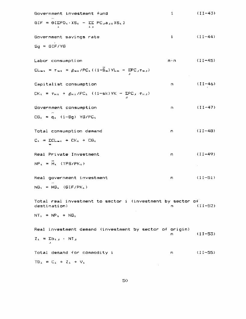
Government investment fund 1 (II-43)

GIF = eCEPD.I , *XS:, - EE PCja.jXSI.I I j

Government savings rate 1 (11-44)

Sg = GIF/YG

Labor consumption min (1I-45)

CL, = T,.. + ± 1a/PCs ( (-S )YL. - EPCj.r...)J

Capitalist consumption n (11-46)

CK' = T-,. + ,. ./PC. ((l-sk)YK - EPC.j T..j)

Government consumption n (II--47)

CGi = qi (1-'Sg) YG/PF'C

Total consumption demand n (11-48)

C. E CL,. + CK. + CGB

Real Private Investment n (I1-49)

NP. = H: (TPS/PK.)

Real government investment n (11-51)

NGi. H= HG G (GIF/PKi)

Total real investment to sector i (investment by sector ofdesti nati on) n (11-52)

NT.I NPi + NGI

Real investment demand (investment by sector of origin)n (11-53)

Z =. = Eb.. * NTj

Total demand for commodity i n (II-55)

TDI = Ci + Zi + V.

50

Domestic use ratio n (II -57)--1

d. = ft (m. , )

Total domest ic demand for domest i c product i on n (11-58)

DC.A d.i * TD,

Total demand for domestic production n (II-59)

XDi = DC, +- E:,

Market clearing n (II-60)

XDi - XSt = 0

Total: 2 n + m + n *m + 8

Endogenous Variables

Nu..mmber'

TSR. , TSA . 2nTotal export subsidy granted under the taxrebate and corporate income tax allowanceschemes, respecti vel y.

TKA Total corporate income tax allowance granted 1

EM I Value of imported intermediate inputs nused for export production

TEMI :L Total tariff cost paid on EMIi n

SE.. Realized combined export subsidy rate n

PWEi Price of the exported domestic good n

E± Foreign demand for exports n

DS) Domestic supply, consumed domestically n

M.J Import demand n

YL. Labor income by type m

51

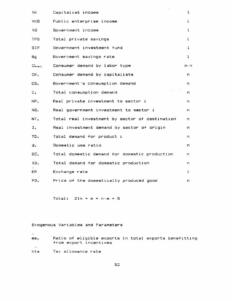
YK Capitalist income 1

YKG Public enterprise income 1

YG Government income 1

TPS Total private savings 1

GIF Government investment fund 1

Sg Government savings rate 1

CLw.t Consumer demand by labor type mn

CK. Consumer demand by capitalists n

CGi Government's consumption demand n

CT Total consumption demand n

NP.i Real private investment to sector i n

NGi Real government investment to sector i n

NT± Total real investment by sector of destination n

Zi Real investment demand by sector of origin n

TDi Total demand for product i n

de Domestic use ratio n

DC, Total domestic demand for domestic production n

XD. Total demand for domestic production n

ER Exchange rate 1

PDI Price of the domestically produced good n

Total: 21n + m + n'm + 8

Exogenous Variables and Parameters

eei Ratio of eligible exports in total exports benefittingfrom export incentives

kta Tax allowance rate

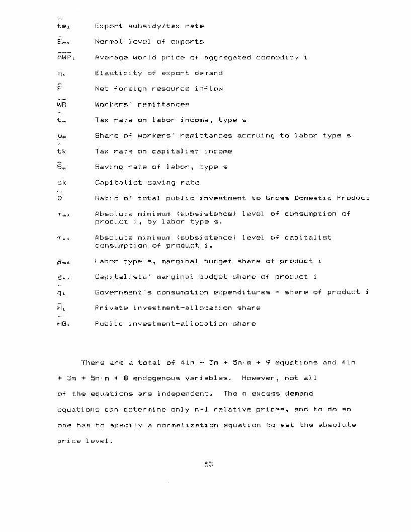
teE. Export subsidy/tax rate

Ec.::i. Normal level of exports

AWF'P Average world price of aggregated commodity i

'q Elast i city of e'x. port demand

F Net foreign resource inflow

WR Workers' remittances

t,, Tax rate on labor income, type s

)i, Share of workers' remittances accruing to labor type s

tk Tax rate on capitalist income

S. Saving rate of labor, type s

sk Capitalist saving rate

6 Ratio of total public investment to Gross Domestic Product

'Tm. Absolute minimum (subsistence) level of consumption ofproduct i, by labor type s.

'j. Absolute m inimum (subsistence) level of capital i stconsumption of product i.

,,. Labor type s, marginal budget share of product i

...• Capita:l. ists' marginal budget share of product i

q, Government's consumption expenditures - share of product i

H:L Frivate investment-allocation share

HG. Public investment-allocation share

There are a total of 41n + 3m + 5n'm + 9 equations and 41n

+ 3m + 5n*m + 8 endogenous variables. However, not all

of the equations are independent. The n excess demand

equations can determine only n-:l relative prices, and to do so

one has to specify a normalization equation to set the absolute

price level.

Footnotes:

(1) For a recent survey on CGE-type Modelling see: Shoven &

Whalley (1984).

(2) My sole purpose in this introduction is to provide a bird's-

eye-view comparison of various multisector planning models. The

interested reader can find a comprehensive survey of Linear

Programming Models in Taylor (1979); and of planning models in

general, in Blitzer, Clark & Taylor (1975).

(3) For a more formal discussion on this proposition, see for

example, Intriligator (1971).

(4) Dervis, de Melo and Robinson, 1982, p. 132. This

observation clearly applies to the general structure of

most of the LP models. Yet, for purposes of completeness

we need to stress the existance of a body of literature

which attempts to compute the competitive market

equilibria by means of extensions of a mathematical

programming model (e.g., see Goreaux (1977); Manne et.al.

(1978); Norton & Scandizzo (1981) ). The Goreaux: and

Manne et. al. studies utilize successive recursive

sequences of linear programming solutions, and can be

regarded as lying halfway between the LP and CGE type

models.

The Norton &. Scandizzo study, on the other hand, tries

to mimic competitive equilibria by directly constructing

the essential conditions of such equilibria as inequality

constraints in the primal problem; and thus, their

procedure can be utilized to yield a non-recursive linear

54

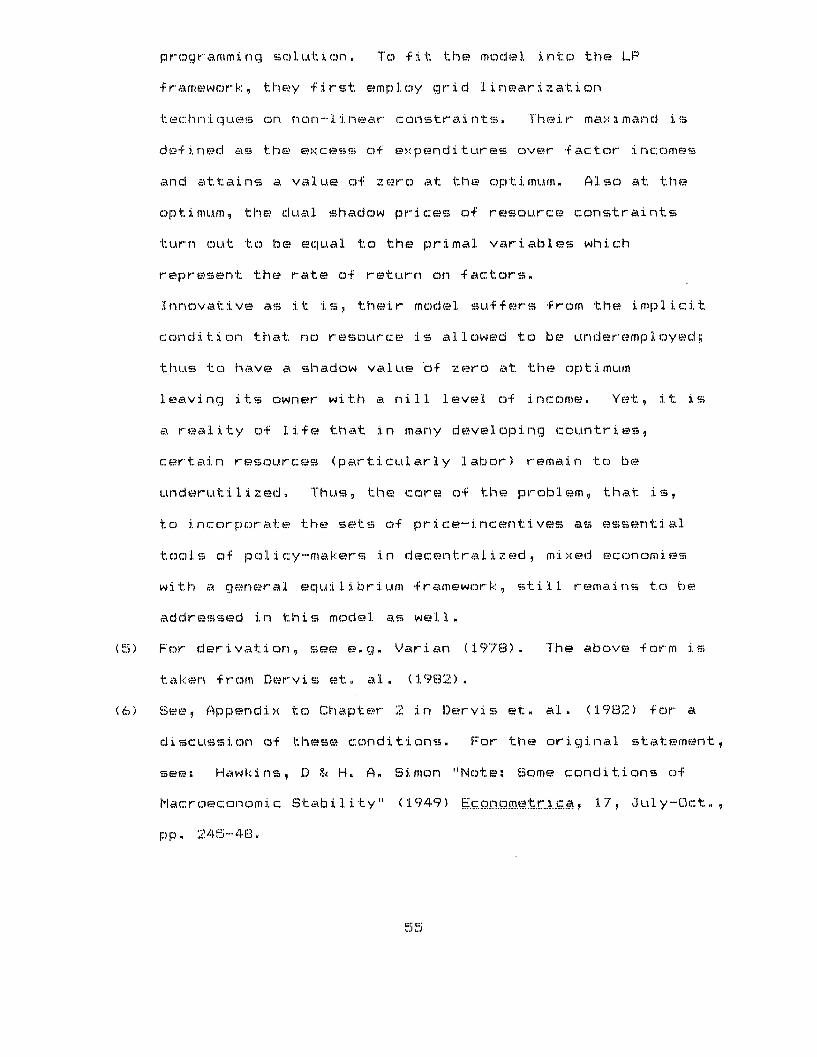
programming solution. To fit the model into the LP

framework, they first employ grid linearization

tec:::hn iq ues on norn inear constraints. TIhei r max i.mand is

de:fined as the excess of ex.penditures over factor inc.omes

and attains a value of zero at the optmumL. Also at the

optimum, the dual shadow prices of resource constraints

turn out to be equal to the primal variables which

represent the rate of return on factors.

Innovative as it is, their model suffers from the implicit

condition that no resource is allowed to be underemployed;

thus to have a shadow value of zero at the optimum

leaving its owner with a nill level of income. Yet, it is

a reality of life that in many developing countries,

certain resources (particularly labor) remain to be

underutilized. Thus, the core of the problem, that is,

to incorporate the sets of price-incentives as essential

tools of poli cy-makers in decentralized, mixed economies

with a general equilibrium framework, still remains to be

addressed in this model as well..

(5) For derivation, see e.g. Varian (1978). The above form is

taken from Dervis et. al. (1982).

(6) See, Appendi x to Chapter 2 in Dervis et al. (1982) for a

discussion of these conditions. For the original statement,

see: Hawkins, D & H. A. Simon "Note: Some conditions of

Macroeconomic Stability" (1.949) E.onEmetrca, 17, J ul y-Oct ,

pp. 245-48B

55=11 91On~

(7) The Model captures such intertemporal innovations in the

Dynamic Stage with the explicit specification of the

endogenous private investment share parameters (see

equations III -5).

(8) For a discussion of various solution strategies and solution

algorithms on the iteration of prices, see Dervis et. al.

(1982, Appendix B); and Adelman and Robinson (1978, Appendix B)

and the references therein cited.

(9) For a discussion on the strategy for construction dynamic,

economy-wide models of developing countries, see Robinson

(1976).

56

References

A d e l m an, I. and S. Robi n s on (:1978) Income Distri but.ion Policies

..D.evelp inr. uritries Lond on: tro Oxford Unr.iversi t.y Preses.'_ ........ e... IJ..............g.............. ... e ..... i.......s. . i o n d C n : O .. o r d U n i v e: r s i t y Fress

Ahluwalia, M.S. and F. J. Lysy (1979) "Welfare Effects of Demand

Management Policies: Impact Multipliers under Alternative

Model Structures", Joyurnal .. of glicy Mode.lling Vol. 1,

No. 3, pp. 317-42.

Arminrgton, '. (1969) "A Theory of Demand for Products

D i st i ngu i sh ed b y P 1 ace aof P ro d ct i. n" .. t..f.. Papers

vol. 16, pp. 159-78.

B i tzer , C., F'. Cl.ark and L. T"ay1or (1975) Ec:ongmy-:Wide• ode..l.

ad.e!D.e.V l .••....:. ....... E.LA ...n ...i. , L.on n d on x3 f o r d iU n i ver si ty Pres s

Cardoso, E. A. and L. Taylor (1979) "Identity-Based Planning of

Prices and Quanttiti es: Cambridge and Neoclassical Models for

Brazil" , Jornal of .Pol. icyodelling, o 1 No. 1, pp. 83-

111.

Der vis, K., J. de Melo and S. Robinson (1982) (eneral_EquiLibrIm

Mogdels Forr Devek. .o menit o.lirv, Cambridge: Cambridge!.... ..... ..............1-.-- ....... .i . . ... . C a m b r i g a m b i d g e

University Press.

Dervis, K. and S. Robinson (1978) "The Foreign Exchange Gap,

Growth a nd Industrial Strategy i n TurkI.:ey: 1973-1983" .' Wo.rld

Bank ... Staff Work.iri.....PaerNo. 306, Washington D Th e

World Bank.

Feltenstein, A. (1980) "A General Equilibrium Approach to the

Analysis of Trade Restrictions, with an Application of

Argentina", IMF Staff Papers., Vol 2'7, No 4, p p . 749-84.

57

Frisch, R. (1959) "A Complete Scheme for Computing All Direct and

Cross Demand Elasticities in a Model with Many Sectors",

Ecn.9nne.tr.i ::_, Vaol. 27, pp. 177-96.

Goreux, L. M. (1977) Interde.endence in Plann. i1n: MultilevelS u..1......f .. ..._d _ . ... ........ I ....a.... . . ......... .... .. !e

Progr.ammi. ti.Studies of the Ivory Coast., Baltimore: Johns

Hopkins Press.

Gupta, S. and S. Togan (1984) "Who Benefits from the Adjustment

Process in Developing Countries? A Test on India, Kenya and

Turkey", Journal of Policy _M.delling, Vol. 6, No. 1,

pp. 95-109.

Harris, J. and M. Todaro (1970) "Migration, Unemployment and

Development: A Two-Sector Analysis". American .Ec.onomic

Revie..w Vol. 60, pp. 126-42.

I ntriligator, M. (1971) Math.ematical Optimization and Economic

TheIory. Englewood Cliffs, N.J.: Prentice-Hall.

Lundborg, P., (1984) "The Nexus Between Income Distribution,

Trade Policy, and Monopoly Power: An Assessment of the

Tin Market", JOLrnal o_ Folicy Modell.ing., Vol. 1, No. 2,

pp. 69-79.

Lewis, J. and S. Urata (1983) "Turkey: Recent Economic

Performance and Medium-Term Prospects, 1978-1990C" World

Bank Staff. Wor.kinagPaperNo. 602 , Washington, D.C.: The

World Bank.

Manne, -A.S., H. P. Chao and R. Wilson (1978) "Computation of

Competitive Equilibrium by a Sequence of Linear Programs",

Department of Operations Research, Stanford University,

January.

58

Melo, M. H. de (1979) "Agr icultural Poli:cies and Development: A

Socioec.onomic Investigation Applied to Sri Lanka" ,Journal.." ".. 1... '7..-.3 1 ..

:... .. '..i. y M...... ........del..li....g Vol. 1 , No. 2, pp. 217-34.

lMe. o, d 3 . de and S. Rob inson (198(0) "The Impact. of "Irade Pol. i cies

on Income Distrribution in a P1lanning Model for Colmb i a",

jurnal ..... 1. lc Model.. , Vol . 2, No. 2, pp . 81-1C 0

Norton, R. D. and P. L.. Scandizzo (1981) "Market Equilibrium

Computations in Activity Analysis Models" QO.Cperat.ions.

RBesearcLh, Vol. 29, No. 2 pp 243-62.

Rob inson, S. (1976) "Towards an Adequate Long'-Ruin Model of: Inc:o:me

Di str i b ut. i o n a nd Economic D evel opment" Ajm.r•.c._ai _! .....Economi•...

Review, Vol 66, Noo. 2, pp, 1.22-7.

Schuh, E. (1976) "Out-Migration, Rural Productivity, and the

Distribution of Income", Paper presented at the World Bank

Conf erence on Rural-Ur-ban Labor Mar:ket Interac ti ots,

Washington, D. C.

Shoven, J. B. and J. Whall.ey (1984) "Applied General-Equilibr ium

Model s o:f " a ti on and Int ernat. ional Tr ade A n In r- o d ..u ct ion

and Survey" , Jurnal ofi Ecgonomic Literature. Vol. 22,

Sep tember, pp. : 1007-51.

T"aylor, L. (1979) MacroI.opodels._for Develop inq Cntries., New

York: Mc3Graw-Hi.11

Taylor, L.. and S. L. Black (1974) "Practical General Equilibrium

Estimation of Resource Pulls Under Trade Liberalization",

Journal of International Economics, Vol. 4,1 pp. 37-58.

Varian, H. (1978) Microeco.nomic na..lsis, New Y o r k : Norton.

59

Appendix A: Derivation of the Linear Expenditure System

In this Appendix I will present the derivation of the

private consumption equations (II-45,-46) in more detail. For

applied work linearity of such equations provides a distinct

advantage and this is one of the reasons of the popularity of

linear expenditure systems (LES). The other advantage of the LES

is that it is relatively easy to estimate its parameters with'

modest data requirements.

This presentation follows that of Taylor (1979); for another

method on deriving linear consumption functions the reader may

refer to the discussion in Adelman & Robinson (1978, Appendix

A). The notation used here pertains on.ly to this Appendix.

First, we begin with the conventional hypothesis that each

consumer group (m - labor categories and capitalists, a total of

m + 1) shares a common utility function and thus, can be analyzed

by the actions of a representative consumer. Dropping the

subscripts s and k that distinguish different consumer

categories, the preference map is assumed to be represented by

the following function:

LU = E .1. log(C - Tr) (A-1)

where C±. is the consumption of i'th commodity and s. and Ti are

the parameters of the utility function. If you recall, I have

let , 3± to stand for the marginal budget share of product i and T.

to denote the "subsistence minima" of product i in physical

t er ms.

60

Assuming non-satiation we can set up the budget constraint

of the representative c'onsumer as an equality,

EP.. ' C-. = Y (A-2)

where Y is the total money income of the consumer and P:. is the

markl:et price of the i -th commodity. The first order conditions

of the consumer's problem yield.

i. ":= XP"'j. (C. -" T..) (A-3)

where > is the f:amil. iar L.agr'ange mul.tiplier.. In our c:ontext we

wi.ll i nterpret it as the "margi nal uti ].i ty of income "

To solve the system (A-3), we will resort to a normalization

rule which states that summatio(n of 1.. over i adds up to unity,

Thus,

1 = X ( = ), (EPiC. - F'. T(. ) (A-4)

Let us denote EF'P..i by S, the total cost of subsistence1.

consumption basket, then from (A-4) we carn solve for X,

S= i/Y-S (A-5)

Substituting (A-5) into (A - 3) we get a specific formula for

demand of commodity i,

C.L = T.- . + ( ./PF'. ) (Y-S) (A-6)

which is the consumption equation I have used in the Model.

Given data on a•.era.ge. budget shares, cX.. (<a.:. = P Ci/Y),

and :i. n come e lastic:ities, 'n... , we can get an estimat e of4

61

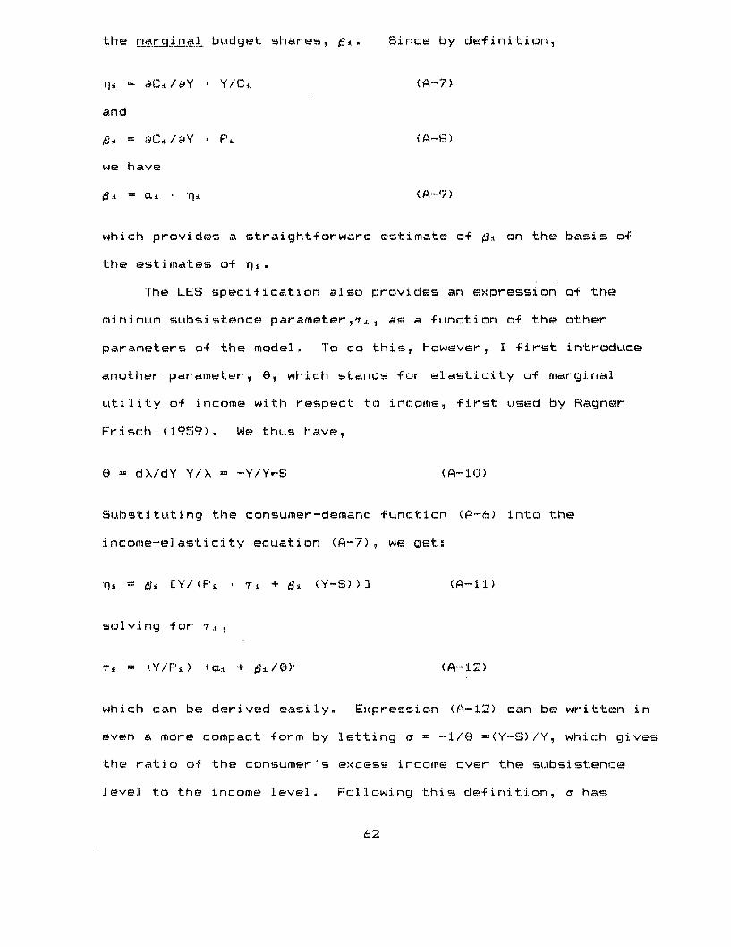
the marginal budget shares, B ,

•i = C / Y ./ * Y/C, (A-7)

and

*t == aC,./aY * F' (A-8)

we have

j. = C L , 'OA (A-9)

which provides a straightforward estimate of ± on the basis of

the estimates of n.i

The LES specification also provides an expression of the

minimum subsistence parameter,To, as a function of the other

parameters of the model. To do this, however, I first introduce

another parameter, 8, which stands for elasticity of marginal

utility of income with respect to income, first used by Ragner

Frisch (1959). We thus have,

8 = dX/dY Y/>, = -Y/YrS (A-10)

Substituting the consumer-demand function (A-6) into the

income-elasticity equation (A-7), we get:

'qi = e Y/(PF' * Ti + (Y-S)) 3 (A-11)

solving for :..,

i = (Y/FP ) (cLi + B<:/e) (A-12)

which can be derived easily. Expression (A-12) can be written in

even a more compact form by letting a = -1/e =(Y-S)/Y, which gives

the ratio of the consumer's excess income over the subsistence

level to the income level. Following this definition, a has

62

Since by definition,

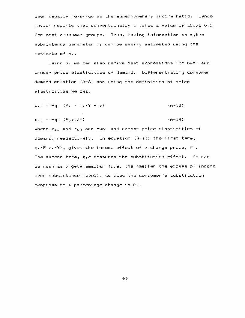
been usually referred as the superenumerary income ratio. Lance

Taylor reports that conventionally a takes a value of about ) .5

for most consutmer groups. Thus, having in f ormat ion on a the

subsistence parameter T. can be easily estimated using the

estimate of i,.

Using a, we can also derive neat expressions for own- and

cross- price el.asticities of demand. Differentiating consumer

demand equation (A-6) and using the definition of price

elasticities we get,

SJ. -'1 : (PF. + r, ./Y + - ) (A-i3)

.j . = -nl. (Pj.r../Y) (A-14)

where e.L and E.L j are own- and cross- price elasticities of

demand, respectively. In equation (A-13) the first term,

SIPL (Pi.. /Y) , gives the income effect of a change price, P,.

The second term, 'r•i. measures the substitution effect. As can

be seen as a gets smaller (i.e. the smaller the excess of income

over subsistence level) , so does the consumer's substitution

response to a percentage change in Pi..

63

Appendix B: Endogenous Derivation of the Own-Price Elasticity

of Domestic Demand

X x:)

In this Appendix we seek for an expression for .. -own

domestic price elasticity of aggregate demand for the domestic

commodity- which can be generated within the Model

endogenously. The calculation of this parameter bears

importance, because for sectors which entail monopoly power in

their product markets, labor hire, and thus, output supply

decisions will depend upon the numerical value of the elasticity

of the total demand curve facing the monopolist. It needs to be

noted that, for the most part, the Appendix is written in the

spirit of a suggestive essay. It needs to be amended in the

realm of the model construction and available data. Of course,XY X.4

ýi can as well be estimated econometrically in a separate study

and can be fed into the Model directly. Yet, this Imethod may be

harder and less reliable than it seems, due to the high level of

aggregation of products in each sector. At such high levels of

aggregation, the econometric fitness and the validity of the

numerical value estimated for :L may be questionable.

Further, since CGE type Models are actually "consistency"

models, it will be a more sound strategy to let the Model

derive its parameters endogenously as much as possible and

to rely less on parameters derived from outside models which use

a different methodology.

There is yet a third possible "method" for finding a value

for s.: , and that is to make an "educated guess" on likely values

64

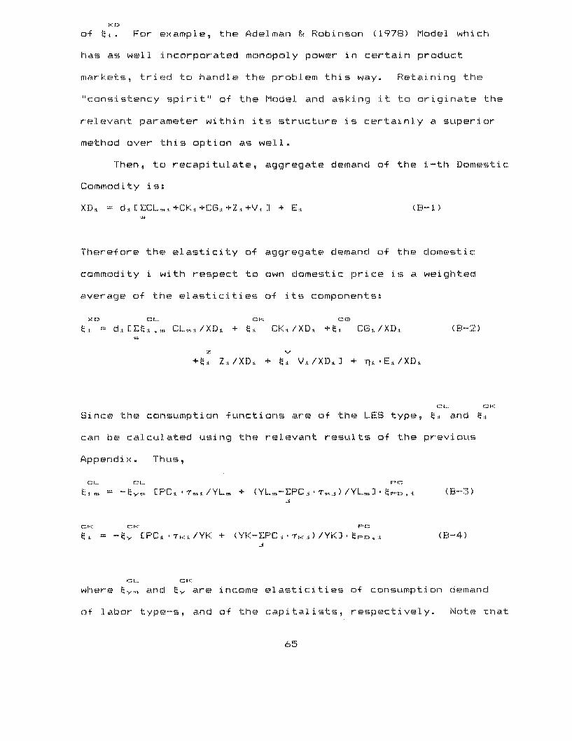
of s.. For example, the Adelman , Robinson (1978) Model which

has as well incorporated monopoly power in certain product

markets, tried to handle the problem this way. Retaining the

"co-nsi. stenc:y spirit" of the Model and asking it to originate the

relevant parameter within its structure is certainly a superior

method over this option as well.

Then, to recapitulate, aggregate demand o-f the i-th Domestic

Commodity is:

XD± = d , ECL .i. +CK J. CG.i +Z .+V. ] + E:< (B-1)

Therefore the elasticity of aggregate demand of the domestic.

commodity i with respect to own domestic price is a weighted

average of the elasticities of its components:

X g. C I.... C. I::. C 03

x D

i. dI > l. d-. C L.i.L /L XI)J ± Cf: / XI) 1 +L x f. ( / ( 41-- 2 1

+si Z. /XD. + 4 i VI /XD,. + '. Ei/XD:)

C1t.... (::;H

Since the co)nsumption functions are o.f the LES type, g:, and E.

can be calculated using the relevant results o.f the previous

Appenedix. Thus,

C, I.... C:, L... F;C" l

.... = -I v-y . EF'C. I /YL,.B + (YL.u-EP'C..j '~,, . )/YL..3 ] , F>., (B-3)

; :: C:; I-:: F (

t = -v, CF'C. , rtK.. /YK + (YK-EPC:F , I r,, ) /YK3 ,-.O, (B-4)

CL.. C.K:

where ,,. and ., are income elasticities of consumption clemand

of :Iabor type-s, and of the capital ists, respectively. Note that

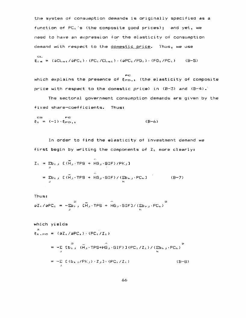
the system of consumption demands is originally specified as a

function of PC~'s (the composite good prices); and yet, we

need to have an expression for the elasticity of consumption

demand with respect to the dom.estic ... price. Thus, we use

t.i . = ( CL. /F'PC ) * (PCi../CL.B ) * (FPC./F'PD. ) (F'PD./PC,. ) (B-5)

which explains the presence of tFOD,± (the elasticity of composite

price with respect to the domestic price) in (B-3) and (8-4).

The sectoral government consumption demands are given by the

fixed share-coefficients. Thus:

0 Mt- F:' C

i (-I) F-DI (B-6)

In order to find the elasticity of investment demand we

first begin by writing the components of Z± more clearly:

Z. = Ebij E (HjTFPS + HGj ,( IF)/PKj]3-i

SEb,. j (Hj*TPS + HGj*'GIF)/( Eb ..,*PCJ (-7)j *I.,

Thus:

9Z./aPC, -= -Eb... CH..jTPS + HG.j, GIF3/(Eb,: , FPC .)j I*:

which yieldsz

s..ZC == (Za./PCFC ) * (PC./Za)

= -E Cbi. (Hj'*TPS+HGj *,GIF) (PCF:',/Z.)/(b<Eb. i.. F'*PC,:).j I-,:

= -E [ (b.,.../PK: ) , Z.. 3 (F'C.. /Z. ) (B-8).i

66

Then, all we need is to solve for:

z r c;::

t.i J . P-, C: ' F . (. - 9')

The demand for inter'med iate goods is given by fi.xed i nput-

output coefficients; and will be assumed to be non-responsive to

price changes.

Actually, any change in the domestic relative prices will

induce an output effec:t and the changing output supply decisi-ons

will result in different quantities of intermediate goods

demanded. ThIhus, we m..st have:

?V.t / PD• : E a,., (<XSj/9F'D,.) (B-10)

where the term in the parantheses (the indirect effect of the

cross-prices on output supp.Lies) can be deduced from the factor

markets through:

SX S. / PD :, ( X S . / L .., ) ( B 1 )

IT E ( L.. / L., .. ) ( d L / d W d . .... ,. * d W .. ,,,/ ld D ) :i*>Ui

The latter component (dL...j,,/dW..i,,; dW.js,/dPD:s.) is embedded in the

solution algorithm for clearing the labor markets and yet is not

observable in a functional formm. In what follows, we are not

able to make use of the functional relationship (B-11 ).

(1) I am indebted to Prof• T". Roe f:or his comments on thispoint.

67

The assumption that the elasticity of intermediate demand isXT)

zero, clearly puts a downward bias on the aggregate value of .

Yet, as we argued, due to the fixed-coefficients technology, the

overall price sensitivity of intermediate demands have to be very

low and the incurred bias shouldnot be substantial.

P'C;

Our final task is to derive an expression for to,- .

Since,

aT (l-a.- ) i.A ( -a• ) 1/I -a.,FPC = 1/B. tE6:. PMi + (1-$.) PD,. J (B-12)

we have

a a i.t9aPCC /sPD = (PC:. /PD ) (l/B.) <(-8<) (B-13)

Thus,

P' C

~t., ... = (PCi. /' FPDL ) (PD /PCF . )

= (PCi/PD,.) (1/Bi) (<-8,.) (B-14)

which completes our derivation. It should be noted, however,

that in spite of its general stance, this exercise still entails

partial equilibrium characteristics. We have not sought for an

expression on the likely general equilibrium effects of PDi on

overall budgets of the economic agents which work through the

factor markets and derived factor incomes. These effects have to

be found in the solution algorithm and the overall interaction of

all markets with a complex set of interlinkages, and technically

68

cannot be identifi ed in a si ng le --or set of-- functi onal form (s).

The inclur'red bias in this manner may or may not be substantial

depending on n the spec :i. f ic ccase at hand and the r-esults snhoauld be

.i nte rpreted wi th c:aut ti on.

69

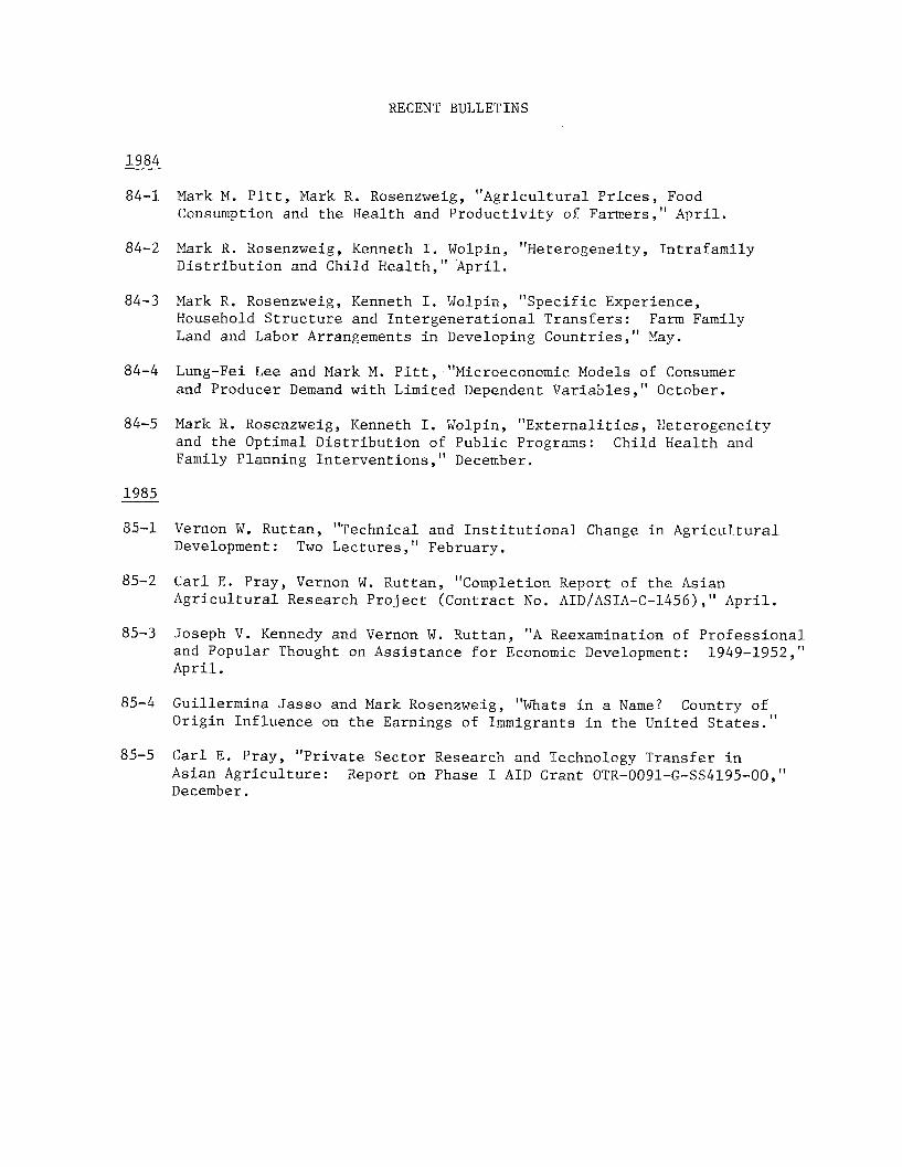
RECENT BULLETINS

1984

84-1 Mark M. Pitt, Mark R. Rosenzweig, "Agricultural Prices, FoodConsumption and the Health and Productivity of Farmers," April.

84-2 Mark R. Rosenzweig, Kenneth I. Wolpin, "Heterogeneity, IntrafamilyDistribution and Child Health," April.

84-3 Mark R. Rosenzweig, Kenneth I. Wolpin, "Specific Experience,Household Structure and Intergenerational Transfers: Farm FamilyLand and Labor Arrangements in Developing Countries," May.

84-4 Lung-Fei Lee and Mark M. Pitt, "Microeconomic Models of Consumerand Producer Demand with Limited Dependent Variables," October.

84-5 Mark R. Rosenzweig, Kenneth I. Wolpin, "Externalities, Heterogeneityand the Optimal Distribution of Public Programs: Child Health andFamily Planning Interventions," December.

1985

85-1 Vernon W. Ruttan, "Technical and Institutional Change in AgriculturalDevelopment: Two Lectures," February.

85-2 Carl E. Pray, Vernon W. Ruttan, "Completion Report of the AsianAgricultural Research Project (Contract No. AID/ASIA-C-1456)," April.

85-3 Joseph V. Kennedy and Vernon W. Ruttan, "A Reexamination of Professionaland Popular Thought on Assistance for Economic Development: 1949-1952,"April.

85-4 Guillermina Jasso and Mark Rosenzweig, "Whats in a Name? Country ofOrigin Influence on the Earnings of Immigrants in the United States."

85-5 Carl E. Pray, "Private Sector Research and Technology Transfer inAsian Agriculture: Report on Phase I AID Grant OTR-0091-G-SS4195-00,"December.