Channel-adaptive Interpolation for Improved Bathymetric TIN

J. K. McGrath1, J. P. O’Kane1, K. J. Barry1, R. C. Kavanagh2

1Department of Civil and Environmental Engineering,

National University of Ireland, Cork (UCC), College Road, Cork, Ireland. Telephone: + 353 21 490 2285

Fax: + 353 21 427 6648 Email: j.k.mcgrath@student.ucc.ie, jpokane@ucc.ie, kjbarry@gmail.com

2Department of Electrical and Electronic Engineering, UCC.

Email: r.kavanagh@ucc.ie

1. Introduction High-resolution, high-frequency data are required for the development of accurate and credible numerical models (Abbot, 1979). In preparing marine topographical data, it is usually necessary to transpose irregularly sampled surfaces to a regularly sampled array. The most popular method to achieve this conversion is to generate a Triangulated Irregular Network (TIN) from the available sample points and to then sample that TIN to produce the regularly-spaced array.

It will be shown that spurious artefacts (pits and lands) may be generated when compiling a TIN from a single-beam bathymetric survey; particularly in the presence of comparatively narrow channels (narrow implies channel width is of a similar magnitude to that of the inter-sample distance). These artefacts may lead to numerical instabilities within the model; particularly if the channels occur in the intertidal zone. The usual response to these artefacts (if identified and problematic) is to apply smoothing convolution filter kernels to the gridded bathymetry until numerical instabilities are overcome. This solution may be adequate in some cases; however, it is deleterious to good data and tolerant of bad. Therefore, it is proposed to employ a new approach in which an adaptive interpolation routine is applied to the original irregularly sampled survey data. This interpolation routine will preferentially interpolate according to the identified channel path. The resulting gridded bathymetric model will be a better approximation to true bathymetry with flow-channels preserved.

2. Triangulation and Channel-adaptive Interpolation Delaunay triangulation methods are well documented and involve the generation of a dense network of triangles with vertices composed of three adjacent sample points. Each triangle defines a 3-dimensional plane in space. A regular grid point takes its value according to its position in such a triangle.

The resulting TIN is a good approximation when the topography is gently sloping, however; abrupt changes in depth may not be synthesised well. Take the example of a TIN generated for Cork Harbour and its ability to represent narrow channels in tidal mudflats in Lough Mahon.

Figure 1: Unconstrained TIN bathymetry of the mudflats at Lough Mahon. Channels in

the mudflats are not correctly resolved.

Figure 2: High-resolution (30 cm pixel) true-colour ortho-image of the same mudflats at

Lough Mahon. When used as input data to a numerical model of the advection and dispersion of

pollution, such as that which has been developed for Cork Harbour, the “unnatural” pits in the mudflat channels, cause instability. To explain the origin of spurious pits, Figure 3a shows a close-up zoom of part of the bathymetry in Figure 1, superimposed with original survey data-points and resulting TIN mesh.

0 200 m

0 200 m

Figure 3a: Mesh of unconstrained TIN triangles and raw sample points. Added lines (blue, purple, yellow) represent locations at which cross-sections were taken to generate Figure 3b.

-0.8-0.6-0.4-0.2

00.20.40.60.8

1

Figure 3b: Poorly resolved flow-channels – plots of channel cross-sections extracted

from Figure 3a.

Three things are apparent from an inspection of Figure 3a: (i) each of the (NE-SW oriented) single beam surveys has a sufficient density of survey points to recover channel information, (ii) the distribution of survey points is isotropic (the inter-sample distance along a beam (~ 6 m) is far shorter than that between survey beams (~ 24 m)), (iii) the triangles making up the TIN do not respect the orientation of the channels. In response to the third point, it is proposed to impose a biased interpolation routine, with a preference to interpolate in the direction of the channel. This requires the identification of the channel. The most reliable and simplest method for doing this is to manually record the path of the channel: see Figure 4.

0 20 m

0 m 150 m

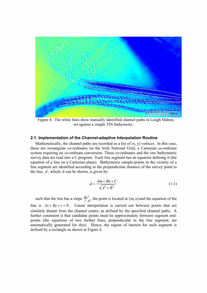
Figure 4: The white lines show manually identified channel paths in Lough Mahon,

set against a simple TIN bathymetry.

2.1. Implementation of the Channel-adaptive Interpolation Routine Mathematically, the channel paths are recorded as a list of (x, y) vertices. In this case,

these are rectangular co-ordinates on the Irish National Grid; a Cartesian co-ordinate system requiring no co-ordinate conversion. These co-ordinates and the raw bathymetric survey data are read into a C program. Each line segment has an equation defining it (the equation of a line on a Cartesian plane). Bathymetric sample-points in the vicinity of a line segment are identified according to the perpendicular distance of the survey point to the line, d , which, it can be shown, is given by:

2 2

Am Bn CdA B+ +

=+

(1.1)

such that the line has a slope B

A , the point is located at ( , )m n and the equation of the

line is 0Ax By c+ + = . Linear interpolation is carried out between points that are similarly distant from the channel centre, as defined by the specified channel paths. A further constraint is that candidate points must lie approximately between segment end-points (the equations of two further lines, perpendicular to the line segment, are automatically generated for this). Hence, the region of interest for each segment is defined by a rectangle as shown in Figure 4.

0 100 m

Figure 5: An example of a selected channel path segment. The rectangle indicates the

region of interest for a particular path segment; the region in which to impose channel-guided interpolation.

In the C Program, the operator has the freedom to define a number of variables,

including: • A nominal channel width; specify which points should be considered for the

channel-adaptive interpolation • A tolerance band; interpolation pairs should be similarly distant from the

centre of the channel • Density of added points; indicate the number of interpolated values to be added

between each interpolation pair

Figure 6: The extra red points represent data points added by the channel-adaptive

interpolation routine. The channel representation in the background bathymetry is significantly improved relative to that in Figure 5.

Figure 7a: Mesh of TIN triangles and sample points following addition of points

generated by channel-guided interpolation. The added lines (blue, purple, yellow) represent locations at which cross-sections were taken to generate plots for Figure 7b.

-0.8-0.6-0.4-0.2

00.20.40.60.8

1

Figure 7b: Cross-sections of the better-resolved flow-channels. These plots compare

well with noisy plots across the same sections as shown in Figure 3b

Significantly, from a software/programming perspective, the chosen implementation is invariant to the method of triangulation (whether Delaunay TIN or Minimum Curvature, etc.). The C Program appends the added points to the raw *.xyz data file which can then be used in the same way as the original data. The implementation is also platform-independent in that the operator can continue to use his/her preferred GIS software for the triangulation procedure. All that is required is a C-compiler.

0 20 m

0 m 150 m

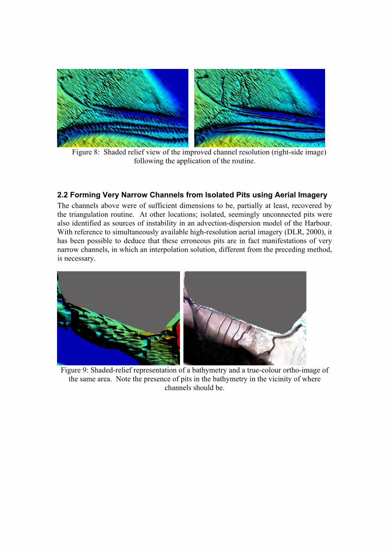
Figure 8: Shaded relief view of the improved channel resolution (right-side image)

following the application of the routine.

2.2 Forming Very Narrow Channels from Isolated Pits using Aerial Imagery The channels above were of sufficient dimensions to be, partially at least, recovered by the triangulation routine. At other locations; isolated, seemingly unconnected pits were also identified as sources of instability in an advection-dispersion model of the Harbour. With reference to simultaneously available high-resolution aerial imagery (DLR, 2000), it has been possible to deduce that these erroneous pits are in fact manifestations of very narrow channels, in which an interpolation solution, different from the preceding method, is necessary.

Figure 9: Shaded-relief representation of a bathymetry and a true-colour ortho-image of

the same area. Note the presence of pits in the bathymetry in the vicinity of where channels should be.

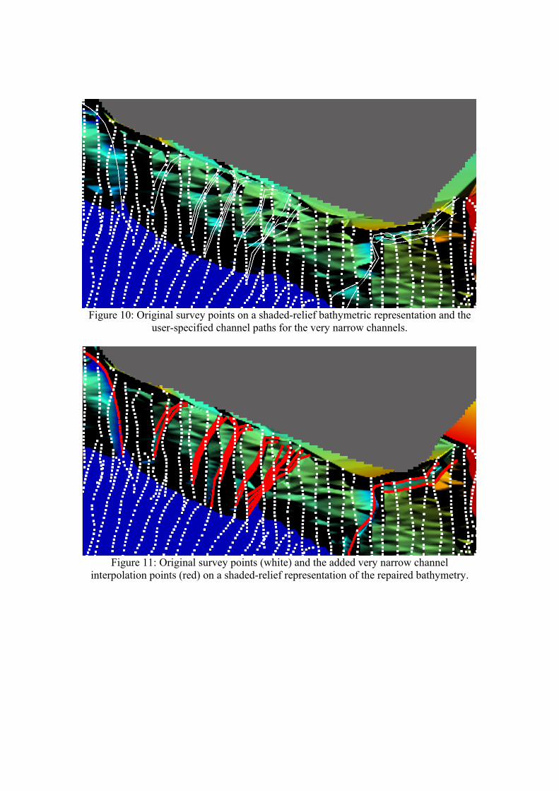
Figure 10: Original survey points on a shaded-relief bathymetric representation and the

user-specified channel paths for the very narrow channels.

Figure 11: Original survey points (white) and the added very narrow channel

interpolation points (red) on a shaded-relief representation of the repaired bathymetry.

Figure 12: Shaded-relief representation of repaired bathymetry with very narrow channels

and a true-colour ortho-image of the same area. Note that the pits present in Figure 8 have now been connected together to form channels.

2.3 Alternative Solutions Modelling systems such as Mike 21 (DHI), handle instability caused by the presence of erroneous pits by allowing the user to convolve gridded topographical data with a low pass filter. This option is undesirable in that the intervention is too late; smoothing data until the channels have been almost smoothed out. The model will be stable, but the bathymetry is a less faithful representation of reality.

ESRI ArcGIS (using 3D Analyst) offers the user the opportunity to specify mass points, breaklines, or polygons to encourage a TIN to recognise the presence of features on land (DTM) topography. The solutions presented here are specialised solutions for resolving flow channels to ensure the stability of a hydrodynamic model reliant on a bathymetry.

3. Acknowledgements Ordnance Survey Ireland funds the work of Jim McGrath.

4. References Abbot, M.B., 1979, Computational Hydraulics, Pitman Publishing Ltd., London, UK. DLR, 2000, High Resolution Stereo Camera – Airborne (HRSC –A, -AX, -AXW) : The First Very High

Resolution Digital Multispectral Stereo Camera for Airborne Remote Sensing of the Earth, Deutsches Zentrum Für Luft- und Raumfahrt, Berlin, Germany.