Boosting Based Multiclass Ensembles and Their Application ...

Boosting Based Multiclass Ensembles and TheirApplication in Machine Learning

PhD Dissertation

Mubasher Baig

2004-03-0040

AdvisorDr. Mian Muhammad Awais

Department of Computer Science

School of Science and Engineering

Lahore University of Management Sciences

Dedicated To

Lahore University of Management Sciences (LUMS)

Lahore, Pakistan

Lahore University of Management Sciences

School of Science and Engineering

CERTIFICATE

I hereby recommend that the thesis prepared under my supervision by Mubasher Baig titled Boost-

ing Based Multiclass Ensembles and Their Application in Machine Learning be accepted in par-

tial fulfillment of the requirements for the degree of Doctor of Philosophy in Computer Science.

Dr. Mian M. Awais (Advisor)

Recommendation of Examiners’ Committee:

Name Signature

Dr. Mian Muhammad Awais (Advisor) ————————————-

Dr. Asim Karim ————————————-

Dr. Shafay Shamail ————————————-

Dr. Ahmad Kamal Nasir ————————————-

Dr. Kashif Javed (External Examiner) ————————————-

Acknowledgements

I am grateful to Dr. Main M. Awais for his supervision, guidance and support for this thesis. I truly

thank him for his generosity and professionalism without which this dissertation could never have

reached the final state. I am also thankful to Dr. Haroon Atiq Babri for an inspiring introduction to

my research area and for teaching me the basic and advanced Machine Learning courses. I would

like to thank Dr. M. A. Mauad, Dr. Ashraf Iqbal, Dr. Asim Karim, Dr. Asim Loan, Dr. Tariq

Jadoon, Dr. Sohaib Khan, Dr. Naveed Irshad, Dr. Zartash Afzal, Dr. Nabeel Mustafa, and all

faculty of LUMS for their inspiring research and effective teaching.

Contents

1 Introduction 1

1.1 Supervised Learning . . . . . . . . . . . . . . . . . . . . . . . . . . . . . . . . . 2

1.2 Ensemble Learning . . . . . . . . . . . . . . . . . . . . . . . . . . . . . . . . . . 3

1.3 Dissertation Contributions . . . . . . . . . . . . . . . . . . . . . . . . . . . . . . 4

1.3.1 Handling Multiclass Learning Problems . . . . . . . . . . . . . . . . . . . 4

1.3.2 Incorporate Domain Knowledge in Boosting . . . . . . . . . . . . . . . . 6

1.3.3 Boosting Based Learning of an Artificial Neural Network . . . . . . . . . 7

1.4 Dissertation Structure . . . . . . . . . . . . . . . . . . . . . . . . . . . . . . . . . 7

1.5 List of Publications . . . . . . . . . . . . . . . . . . . . . . . . . . . . . . . . . . 9

2 Preliminaries 10

2.1 PAC Model of Learning . . . . . . . . . . . . . . . . . . . . . . . . . . . . . . . 11

2.2 Review of Boosting Algorithms . . . . . . . . . . . . . . . . . . . . . . . . . . . 16

2.2.1 AdaBoost Algorithm . . . . . . . . . . . . . . . . . . . . . . . . . . . . . 16

2.2.2 Multi-class Boosting Algorithms . . . . . . . . . . . . . . . . . . . . . . . 18

2.2.3 Incorporating Prior Knowledge in Boosting Procedures . . . . . . . . . . . 20

2.3 Closure Properties of PAC learnable Concept Classes . . . . . . . . . . . . . . . . 20

2.4 Learning Multiple Concepts . . . . . . . . . . . . . . . . . . . . . . . . . . . . . 20

2.4.1 m-PAC Learning . . . . . . . . . . . . . . . . . . . . . . . . . . . . . . . 21

v

3 Multiclass Ensemble Learning 23

3.1 Introduction . . . . . . . . . . . . . . . . . . . . . . . . . . . . . . . . . . . . . . 23

3.2 Multi-Class Boosting Contributions . . . . . . . . . . . . . . . . . . . . . . . . . 25

3.2.1 M-Boost Algorithm . . . . . . . . . . . . . . . . . . . . . . . . . . . . . . 26

3.2.2 CBC: Cascade of Boosted Classifier . . . . . . . . . . . . . . . . . . . . . 33

3.3 Experimental Settings and Results . . . . . . . . . . . . . . . . . . . . . . . . . . 36

3.3.1 M-Boost vs State-of-the-art Boosting Algorithms . . . . . . . . . . . . . . 37

3.3.2 Cascade of Boosted Classifiers for Intrusion Detection . . . . . . . . . . . 42

3.4 Summary . . . . . . . . . . . . . . . . . . . . . . . . . . . . . . . . . . . . . . . 51

4 Incorporating Prior into Boosting 54

4.1 Introduction . . . . . . . . . . . . . . . . . . . . . . . . . . . . . . . . . . . . . . 55

4.2 Incorporating Prior into Boosting . . . . . . . . . . . . . . . . . . . . . . . . . . . 58

4.2.1 Generating the Prior Knowledge . . . . . . . . . . . . . . . . . . . . . . . 62


4.3.1 Results and Discussion . . . . . . . . . . . . . . . . . . . . . . . . . . . . 65

4.4 Summary . . . . . . . . . . . . . . . . . . . . . . . . . . . . . . . . . . . . . . . 69

5 Boosting Based ANN Learning 73

5.1 Introduction . . . . . . . . . . . . . . . . . . . . . . . . . . . . . . . . . . . . . . 74

5.2 AdaBoost Based Neural Network Learning . . . . . . . . . . . . . . . . . . . . . 77

5.2.1 Boostron: Boosting Based Perceptron Learning . . . . . . . . . . . . . . . 78

5.2.2 Beyond a Single Perceptron Learning . . . . . . . . . . . . . . . . . . . . 80

5.2.3 Incorporating Non-Linearity into Neural Network Learning . . . . . . . . 85

5.2.4 Multiclass Learning . . . . . . . . . . . . . . . . . . . . . . . . . . . . . 87

5.3 Learning Artificial Neural Network for Intrusion Detection . . . . . . . . . . . . . 87


vi

5.4.1 Results . . . . . . . . . . . . . . . . . . . . . . . . . . . . . . . . . . . . 91

5.4.2 Artificial Neural Network Based Network Intrusion Detection System . . . 95

5.5 Summary . . . . . . . . . . . . . . . . . . . . . . . . . . . . . . . . . . . . . . . 102

6 Conclusions and Future Research Directions 105

6.1 Limitations and Future Research Directions . . . . . . . . . . . . . . . . . . . . . 107

6.1.1 Incorporating Prior into Boosting . . . . . . . . . . . . . . . . . . . . . . 107

6.1.2 Boosting-Based ANN learning methods . . . . . . . . . . . . . . . . . . . 108

6.1.3 Muulticlass Ensemble Learning . . . . . . . . . . . . . . . . . . . . . . . 109

vii

List of Figures

3.1 Weight reassignment strategy

(a) Relationship of entropy and probability assigned to the actual class . . . . . . . 32

3.2 Hierarchical Structures . . . . . . . . . . . . . . . . . . . . . . . . . . . . . . . . 35

3.3 Effect of weight vector α on the test error of AdaBoost-M1 . . . . . . . . . . . . . 40

3.4 Error rate comparison of M-Boost, Multi-Class AdaBoost and AdaBoost-MH . . . 43

3.5 Number of datasets per test error interval . . . . . . . . . . . . . . . . . . . . . . . 44

3.6 Test error rate comparison of M-Boost,Gentle, Modest and Real AdaBoost on 4

simulated binary data sets . . . . . . . . . . . . . . . . . . . . . . . . . . . . . . . 45

3.7 Test error rate comparison of M-Boost, Gentle, Modest and Real AdaBoost on 3

binary data sets from UCI repository . . . . . . . . . . . . . . . . . . . . . . . . . 46

3.8 Dataset Statistics . . . . . . . . . . . . . . . . . . . . . . . . . . . . . . . . . . . 48

4.1 Test Error: AdaBoost-P1 vs Multiclass AdaBoost . . . . . . . . . . . . . . . . . . 68

4.2 Test Error: AdaBoost-P1 vs AdaBoost-M1 . . . . . . . . . . . . . . . . . . . . . . 70

4.3 Test Error: Effect of Prior in case of Sparse Training Data . . . . . . . . . . . . . . 71

5.1 Typical structure of a single-layer Perceptron . . . . . . . . . . . . . . . . . . . . 75

5.2 Feed-forward Network with a single hidden layer and a single output unit . . . . . 81

viii

List of Tables

3.1 Datasets used in our experiments . . . . . . . . . . . . . . . . . . . . . . . . . . . 38

3.2 AdaBoost-M1 Vs AdaBoost-M1 with weight vector α . . . . . . . . . . . . . . . . 41

3.3 Percent error rate comparison of M-Boost, AdaBoost-MH and Multi-Class AdaBoost 44

3.4 Dataset Summary: Category, Notation, Name, Type, Statistics and Description . . . 49

3.5 Dataset Summary: Category, Notation, Name, Type, Statistics and Description . . . 50

3.6 Comparison of various methods in terms of accuracy, precision, recall and F1 mea-

sure for training and testing . . . . . . . . . . . . . . . . . . . . . . . . . . . . . . 52

3.7 Comparison of various methods in terms of accuracy, precision, recall and F1 mea-

sure for training and testing . . . . . . . . . . . . . . . . . . . . . . . . . . . . . . 52

4.1 Datasets Used in Our Experiments. . . . . . . . . . . . . . . . . . . . . . . . . . . 66

4.2 Test Error rate Comparison of Multiclass AdaBoost and AdaBoost-P1 . . . . . . . 66

4.3 Test Error rate Comparison of Multiclass AdaBoost and AdaBoost-P1 . . . . . . . 66

4.4 Test Error rate Comparison of AdaBoost-M1 and AdaBoost-P1 . . . . . . . . . . . 69

4.5 Test Error rate Comparison of AdaBoost-M1 and AdaBoost-P1 . . . . . . . . . . . 71

4.6 Effect of Prior Quality on Error rate of Multiclass AdaBoost . . . . . . . . . . . . 71

5.1 Description of Datasets . . . . . . . . . . . . . . . . . . . . . . . . . . . . . . . . 90

5.2 Test Error Rate Comparison of Perceptron vs Boostron . . . . . . . . . . . . . . . 92

5.3 Test Error Rate Comparison of Extended Boostron vs linear Back-propagation . . . 93

ix

5.4 Boosting Based ANN Learning vs Back-propagation Algorithm . . . . . . . . . . 94

5.5 KDD-cup class frequencies . . . . . . . . . . . . . . . . . . . . . . . . . . . . . . 96

5.6 UNSW-NB15 class frequencies . . . . . . . . . . . . . . . . . . . . . . . . . . . . 96

5.7 Performance of Intrusion Detection System for Three Dominant Classes . . . . . . 98

5.8 An average of the performance measures . . . . . . . . . . . . . . . . . . . . . . . 99

5.9 Normal vs Intrusion . . . . . . . . . . . . . . . . . . . . . . . . . . . . . . . . . . 99

5.10 Fold-wise Test Performance . . . . . . . . . . . . . . . . . . . . . . . . . . . . . 100

5.11 Test Performance for 8 Classes Constituting 99.65% of Examples . . . . . . . . . 101

5.12 Test Performance for UNSW-NB15 dataset . . . . . . . . . . . . . . . . . . . . . 101

5.13 Normal vs Intrusion . . . . . . . . . . . . . . . . . . . . . . . . . . . . . . . . . . 102

5.14 Performance Difference of Proposed and Standard ANN for UNSW-NB15 dataset . 103

x

Abstract

Boosting is a generic statistical process for generating accurate classifier ensembles from only

a moderately accurate learning algorithm. AdaBoost (Adaptive Boosting) is a machine learning

algorithm that iteratively fits a number of classifiers on the training data and forms a linear com-

bination of these classifiers to form a final ensemble. This dissertation presents our three major

contributions to boosting based ensemble learning literature which includes two multi-class ensem-

ble learning algorithms, a novel way to incorporate domain knowledge into a variety of boosting

algorithms and an application of boosting in a connectionist framework to learn a feed-forward

artificial neural network.

To learn a multi-class classifier a new multi-class boosting algorithm, called M-Boost, has

been proposed that introduces novel classifier selection and classifier combining rules. M-Boost

uses a simple partitioning algorithm (i.e., decision stumps) as base classifier to handle a multi-class

problem without breaking it into multiple binary problems. It uses a global optimality measures for

selecting a weak classifier as compared to standard AdaBoost variants that use a localized greedy

approach. It also uses a confidence based reweighing strategy for training examples as opposed

to standard exponential multiplicative factor. Finally, M-Boost outputs a probability distribution

over classes rather than a binary classification decision. The algorithm has been tested for eleven

datasets from UCI repository and has consistently performed much better for 9 out of 11 datasets

in terms of classification accuracy.

Another multi-class ensemble learning algorithm, CBC: Cascaded Boosted Classifiers, is also

presented that creates a multiclass ensemble by learning a cascade of boosted classifiers. It does

not require explicit encoding of the given multiclass problem, rather it learns a multi-split decision

tree and implicitly learns the encoding as well. In our recursive approach, an optimal partition of

all classes is selected from the set of all possible partitions and training examples are relabeled.

The reduced multiclass learning problem is then learned by using a multiclass learner. This proce-

dure is recursively applied for each partition in order to learn a complete cascade. For experiments

we have chosen M-Boost as the multi-class ensemble learning algorithm. The proposed algo-

rithm was tested for network intrusion detection dataset (NIDD) adopted from the KDD Cup 99

(KDDâAZ99) prepared and managed by MIT Lincoln Labs as part of the 1998 DARPA Intrusion

Detection Evaluation Program.

To incorporate domain knowledge into boosting an entirely new strategy for incorporating

prior into any boosting algorithm has also been devised. The idea behind incorporating prior into

boosting in our approach is to modify the weight distribution over training examples using the

prior during each iteration. This modification affects the selection of base classifier included in the

ensemble and hence incorporate prior in boosting. Experimental results show that the proposed

method improves the convergence rate, improves accuracy and compensate for lack of training

data.

A novel weight adaptation method in a connectionist framework that uses AdaBoost to mini-

mize an exponential cost function instead of the mean square error minimization is also presented

in this dissertation. This change was introduced to achieve better classification accuracy as the

exponential loss function minimized by AdaBoost is more suitable for learning a classifier. Our

main contribution in this regard is the introduction of a new representation of decision stumps that

when used as base learner in AdaBoost becomes equivalent to a perceptron. This boosting based

method for learning a perceptron is called BOOSTRON. The BOOSTRON algorithm has also been

extended and generalized to learn a multi-layered perceptron. This generalization uses an iterative

strategy along with the BOOSTRON algorithm to learn weights of hidden layer neurons and output

neurons by reducing these problems into problems of learning a single layer perceptron.

ii

Chapter 1

Introduction

Classification refers to the assignment of one or more labels, from a discrete set of labels, to an

object of interest. For example, a voice activity detector used in speech coding systems assigns a

positive label to all speech frames that contain human voice activity and a negative label to frames

that contain background noise. An automatic cancer detection system might classify a medical

image as benign or malignant. An Optical Character Recognition system assigns to each segment

of an image a label from the set of printable UNICODE characters.

A method or program that can assign one or more labels to a given object is known as a clas-

sifier. A numerus set of systems need classifier(s) as a subcomponents to perform some useful

operations. Common examples of such systems include automatic speech recognition and coding,

spam detection, intrusion detection in computer networks, object detection in an image, handwrit-

ten character and digit recognition, automatic detection of disease, automatic fraud detection in

an online transection, document classification, human activity recognition, trend prediction in a

shares market, and object tracking systems etc.

While human beings are extremely good at classifying objects, the task of writing computer

programs for automatic classification proved out to be nontrivial. Learning from experience is a

fundamental ability of all living objects and especially the human cognition system demonstrates

1

an excellent example of a system that learns from past experience. The areas of Artificial intelli-

gence, machine learning, and pattern recognition have devised several computational realizations

of learning behaviour as demonstrated by living organisms. Developing useful methods for cre-

ating a classifier has been the single most important task that lies at the heart of learning from

experience and hence has resulted into several computational methods for building a classifier

under various learning settings.

1.1 Supervised Learning

A common framework for creating a classifier assumes that the classifier learning method takes

as input a set of pre-labeled objects. The learning method then uses these objects and the corre-

sponding labels to learn a classifier of a given form that can be used to assign correct labels to

previously unseen objects. This paradigm for automatic learning of a classifier from a set of la-

beled training examples is commonly referred to as supervised learning as it assumes that objects

have been pre-labeled by an expert supervisor, who is commonly a human. In this learning setting

each object x, commonly represented as a vector of measurements called features, is known as in

instance whereas the set of all possible instances is called the instance space and is denoted as X.

The instance x along with it’s actual label y is represented as an ordered pair (x, y) and is called a

training example.

Thus the supervised learning paradigm assumes that there is an unknown function, f(x), that

maps an instance x to its’ actual label y. A learning method L, called a learner, is provided with a

set of N training examples of the form (x1, y1), ..., (xN , yN) where xi is a vector representing the

object of interest in some n-dimensional instance space X and yi is its’ actual label. The learning

algorithm is required to use the available training data for computing a hypothesis function H(x)

that can approximate the unknown functional relation between the instance space X and the set

of labels. Quality of the learned hypothesis and hence that of the learner L can be estimated

2

by computing it’s performance on a separate set of test examples which is usually referred to as

the test accuracy of learned classifier. Some of the well studied supervised learning algorithms

include neural networks [72, 75], decision tree learning [32, 16], support vector machines [87,

93], probabilistic learning [19, 67], nearest-neighbour classifiers [21], and ensemble learning [10,

13, 27, 33, 35, 84, 91, 103] etc. These algorithms have been successfully used to build several

important systems of practical interest [65, 66, 70, 83, 95, 98].

1.2 Ensemble Learning

Ensemble learning has been one of the most active and applied area of research in the last two

decades [25]. An ensemble of classifiers combines the outputs of several, usually homogenous,

classifiers in some way (e.g. weighted majority voting or averaging) to produce a combined de-

cision about the class of an instance. In particular, Bagging [13] and Boosting [33] are the two

most popular ensemble learning methods in the machine learning literature. Bagging approach of

Breiman [13] selects several instances of a classifier by using bootstrap samples and compute the

final output by taking a simple average of individual classifier outputs. The sampling and averag-

ing steps of bagging tend to reduce the overall variance in classification and hence improves the

performance of the classifier [14, 26, 36].

Boosting based method, like AdaBoost [33], on the other hand maintains an adaptive weight

distribution Dt over training examples and use a learning algorithm to generate a classifier ht

that has optimal performance with respect to Dt. This distribution is modified after generating

each classifier such that the weight of examples misclassified by the classifier ht are increased and

weights of correctly classified examples are decreased. The final classifier,H(x) =∑T

t=1 αt.ht(x),

is formed by taking a linear combination of selected classifiers where the weight αt of classifier ht

in the linear combination depends on its’ training performance with respect to the distribution Dt

used to generate it.

3

AdaBoost based ensembles perform specially well when the individual classifiers have uncor-

related error and their accuracy is guaranteed to be better than random guessing. Particularly, In

the PAC setting, a boosting based ensemble of classifiers is guaranteed to have arbitrarily low error

if the base learning algorithm grantees an accuracy better than random guessing on every weight

distribution maintained on the training examples. Chapter 2 provides a detailed review of PAC

model of Learning, AdaBoost algorithm and introduces its’ several variants.

1.3 Dissertation Contributions

This dissertation presents our three orthogonal contribution in the area of ensemble learning which

includes

1. Two ensemble learning algorithms to handle multiclass learning problems.

2. A novel method to incorporate prior into a large class of boosting algorithms.

3. Boosting based learning of a feed-forward artificial neural network.

1.3.1 Handling Multiclass Learning Problems

Variants of AdaBoost that can handle multi-class problems usually follow two approaches; in the

first approach the algorithms use a multi-class learner (such as decision trees) to generate the

base classifiers, and in the second approach the algorithms break the multi-class learning problem

into several, usually orthogonal, binary classification problems. Each binary sub-problem is then

independently learned by using the binary version of the boosting algorithm and there outputs are

combined to form a multi-class ensemble. We have developed two new methods, M-Boost [5] and

CBC: Cascade of Boosted Classifiers [6], for learning a multiclass ensemble.

4

M-Boost Algorithm

M-Boost algorithm uses a simple partitioning algorithm (i.e., decision stumps) as base classifier to

handle multiclass problem without breaking it into multiple binary problems. This required con-

siderable modifications to the standard AdaBoost. The changes made to AdaBoost pertained to

the way a weak classifier is selected for addition into the ensemble, training example reweighing

strategy, and the way a classifier outputs its classification decision. The new algorithm was imple-

mented, tested, and compared with existing algorithms. Following are the novel features presented

in the new M-Boost algorithm that make it different from the existing algorithms:

Classifier Selection: M-Boost uses a global optimality measures for selecting a weak learner as

compared to standard AdaBoost variants that use a localized greedy approach.

Example Reweighing: M-Boost uses entropy and probability based feature reweighing strategy

for training examples as opposed to standard exponential multiplicative factor.

Combining Classifiers: M-Boost outputs a probability distribution over all classes rather than a

binary classification decision.

M-Boost was tested for several datasets from UCI repository [56] of machine learning datasets

and has consistently performed much better than the two corresponding boosting algorithms,

AdaBoost-M1 [33] and Multi-class AdaBoost [103] in terms of classification accuracy.

CBC: Cascade of Boosted Classifiers

CBC: Cascaded Boosted Classifiers is a generalized approach of creating a multiclass classifier by

using an implicit encoding the classes. It is different from the remaining methods in the sense that

earlier encoding based approaches required an explicit division of multiclass problem into several

independent binary sub-problems whereas CBC does not require such an explicit encoding, rather

it learns a multi-split decision tree and hence implicitly learns the encoding as well. In this recur-

5

sive approach, an optimal partition of all classes is selected from the set of all possible partitions

of classes. The training data is relabeled so that each class in a given partite gets the same label.

The newly labeled training data, typically, has smaller number of classes than the original learning

problem. The reduced multiclass learning problem can now be learned through applying any mul-

ticlass algorithm. For experiments we have chosen M-Boost as the multi-class ensemble learning

algorithm. In order to learn the complete problem, the above mentioned procedure is repeatedly

applied for each partition. The method has been applied to successfully build an effective network

intrusion detection system.

1.3.2 Incorporate Domain Knowledge in Boosting

In most real world situations, significant domain knowledge is available that can be used to further

improve the accuracy and convergence of boosting. An existing approach by Schapire et al. [82]

uses domain knowledge to generate a prior and use it to compensate for lack of training data by

introducing new training examples into the training dataset. Main shortcomings of this approach

are:

1. The impact of prior is significantly low when enough training data is available.

2. There is no effect of introducing prior on the convergence rate of the boosting algorithm.

3. The strategy for incorporating prior is specific to a fixed boosting algorithm and cannot be

applied to all boosting algorithms, in general.

We have devised an entirely new strategy for incorporating prior into any boosting algorithm

that overcomes all the aforementioned limitations of the existing approach. The idea behind incor-

porating the prior into boosting in our approach is to modify the weight distribution over training

examples using the prior during each iteration. This modification affects the selection of base clas-

sifier included in the ensemble and hence incorporate prior in boosting. The results show improved

6

convergence rate, improved accuracy and compensation for lack of training data irrespective of the

size of the training dataset.

1.3.3 Boosting Based Learning of an Artificial Neural Network

We have proposed a new weight adaptation method in a connectionist framework that minimizes

exponential cost function instead of the mean square error minimization, which is the standard

used in most of the perceptron/neural network learning algorithms. We introduced this change

with the aim to achieve better classification accuracy.

Our main contribution in this regard has been a new representation of decision stumps that when

used as base learner in AdaBoost becomes equivalent to a perceptron and is called BOOSTRON

[7]. BOOSTRON has been extended and generalized to learn a multi-layered perceptron with linear

activation function [8]. This generalized method has been used to learn weights of a feed-forward

artificial neural network having linear activation functions, a single hidden layer of neurons and

one output neuron. It uses an iterative strategy along with the BOOSTRON algorithm to learn

weights of hidden layer neurons and output neurons by reducing these problems into problems of

learning a single layer perceptron. Further generalizations of this method resulted into a learning

of a feed-forward artificial neural network that uses non-linear activation function and has multiple

output neurons.

1.4 Dissertation Structure

This dissertation has been organized into six chapters that include this introductory chapter fol-

lowed by chapter 2 that provides the preliminaries definitions and concepts related to ensemble

learning. A detailed account of PAC-learning, boosting and AdaBoost algorithm along with short

descriptions of several practical boosting and ensemble learning algorithms is also presented in

chapter 2. The chapter also lays down the foundation for the remaining chapters by identifying

7

some of the open problems that have been addressed in the remaining chapters.

Details of our new boosting style procedure, M-Boost, for learning multiclass ensemble with-

out breaking the problem into multiple binary classification problems are presented in chapter 3.

Discussion of M-Boost is succeeded with the presentation of a naive method of constructing a

CBC (i.e. Cascade structure of Boosted Classifiers) for learning a multiclass decision tree like

structure. Chapter 3 also presents applications and comparison of M-Boost and CBC with state-of-

the-art boosting algorithms using several commonly referred datasets from the machine learning

literature.

Chapter 4 presents an effective way of incorporating prior into boosting based ensembles. Ex-

perimental results, on several synthetic and real datasets, are also provided in that chapter that

provide empirical evidence of the methods’ effectiveness. These results show significant improve-

ment when the domain knowledge, provided by experts in the form of rules or extracted from the

data, is incorporated into boosting. Proposed method mitigates the necessity of large training data

and improves the convergence and performance of a large family of boosting algorithms.

A novel boosting based perceptron learning algorithm, BOOSTRON, is presented in chapter

5 that uses AdaBoost along with a new representation of decision stumps by using homogenous

coordinates. The chapter also presents several extensions of BOOSTRON for learning a multi-

layer feed-forward artificial neural network with linear and non-linear activation functions. This

chapter concludes with the detailed experimental settings and the corresponding results used to

compare the performance of proposed methods with standard neural network learning algorithms

including the perceptron learning algorithm and error back-propagation learning.

Finally, chapter 6 concludes the discussion by summarizing our contributions and providing

some of the future research directions.

8

1.5 List of Publications

Following publications have resulted from our research work presented in this dissertation.

1. Baig, M., and Mian Muhammad Awais. "Global reweighting and weight vector based strat-

egy for multiclass boosting." Neural Information Processing. Springer Berlin Heidelberg,

2012.

2. Baig, Mubasher, El-Sayed M. El-Alfy, and Mian M. Awais. "Intrusion detection using a

cascade of boosted classifiers (CBC)." Neural Networks (IJCNN), 2014 International Joint

Conference on. IEEE, 2014.

3. Baig, Mirza M., Mian M. Awais, and El-Sayed M. El-Alfy. "BOOSTRON: Boosting Based

Perceptron Learning." Neural Information Processing. Springer International Publishing,

2014.

4. Baig, Mirza Mubasher, El-Sayed M. El-Alfy, and Mian M. Awais. "Learning Rule for Linear

Multilayer Feedforward ANN by Boosted Decision Stumps." Neural Information Process-

ing. Springer International Publishing, 2015.

9

Chapter 2

Preliminaries

Concept learning or binary classification has been at the core of machine learning. A concept is a

partition of an underlying domain of instances, X , into two disjoint parts Xc and Xc. This chapter

introduces the PAC model of learning which provides a theoretical foundation for concept learning.

Following the discussion of PAC model, the chapter presents some it’s extensions including the

weak model of learning. The most important idea of the equivalence of weak and PAC learnability

is also presented that resulted into several early boosting and ensemble learning algorithms.

Discussion of the relevant learning models and the introduction of concept boosting is is suc-

ceeded with a brief review of AdaBoost and some of the related concept boosting algorithms.

AdaBoost algorithm is a concept boosting algorithm and hence can be used to create binary clas-

sifiers only. This chapter also presents some of the extensions of basic AdaBoost algorithm which

can be used to handle multiclass learning problems. This brief review of boosting literature is

succeeded by the presentation of our proposed model,M−PAC model to handle learnability of

a multi-class classifiers

10

2.1 PAC Model of Learning

This section provides a brief overview of the PAC model of learning [92] and also reviews some

important extensions of the learning model. The PAC (Probably Approximately Correct) model

gives a precise meaning to the notion of learnability of a concept c and to that of a class of concepts

C. Learning protocol of the PAC model assumes that a learning algorithm L has access to an

example oracle EX(c;D). L uses the oracle to obtain labeled points (x, c(x)) sampled from

the domain of a concept c. These labeled points are called training examples and are assumed

to be chosen independently from the domain by using a fixed but unknown distribution D. The

labels, c(x), of the instances are assumed to be computed using an unknown concept c. Given

these training examples, the job of L is to accurately estimate the unknown concept c using some

approximate representation of concepts in C. A concept class C is said to be learnable by an

approximate representation of it’s concepts if an algorithm exists that can accurately and efficiently

learn every concept c ∈ C.

A formal definition of PAC learning uses the notions of an instance space, a concept class,

representation and size of a concept, and the notion of a hypotheses space.

An instance space X is a set of encodings of all objects of interest and is the domain of a set of

concepts. For example, X might be encoding of all Boolean valued functions or it might be a set

representing all patients in a hospital where each patient is represented as an ordered pair of some

measured features.

A concept c is a subset of the instance space X and is equivalently defined as a characteristic

function Xc or as a Boolean function defined on the instance space. A concept c defined on an

instance space X partitions it into two disjoint subsets. For example the set of all patients suffering

from a certain disease defines a concept.

A concept class C is a collection of concepts defined on an instance space X . Often the concept

class is subdivided into disjoint subclasses Cn where n = 1, 2, . . . such that the concept class C is

11

the union of the subclasses Cn and all the concepts in Cn are defined on a common domainXn ⊂ X .

For examples, if the concept class C is the set of all boolean formulas then Cn might denote all

Boolean formulas having exactly n variables and Xn will denote the truth assignments to the n

variables. The subscript n typically denotes the size or complexity of the concepts in Cn. It is

important to note that the size of a concept is measured assuming some reasonable representation

of the concept. For example, if the instance space is X = {0, 1}n and the concept to be represented

is a boolean function of n variables then this concept can either be represented as a truth table or

as a simplified formula in n boolean variables. Clearly the size of representation when such a

concept is represented as a truth table is exponentially larger than the size of representation if it is

represented as a simplified function of n boolean variables.

Another important notion used in the definition of PAC model is that of the representation of

hypotheses space H. The estimate of a concept generated by the learning algorithm L is called

a hypothesis and is denoted as h. The set of all possible hypotheses that might be generated by

L is called a hypotheses space of the learning algorithm. Separate representation of a concept

c and that of a hypothesis h is important as the learnability of a concept class C depends on the

representation of hypotheses class H as well. For example, the concept class of all 3-term DNF

formula is not efficiently PAC learnable if the learning algorithm produces a 3-term DNF formula

as the hypothesis but it is efficiently PAC learnable if the learning algorithm is allowed to output a

3-term formula in CNF form [52]. Given the above notions, the PAC model can be fomally defined

as given by Kearns and Vazirani [52]

Definition 2.1.1. A concept class C defined over an instance space X is said to be PAC learnable

using a hypothesis classH if there exists an algorithm L such that for every 0 < ε ≤ 12, 0 < δ ≤ 1

2,

concept c ∈ C, and distribution D over X , the algorithm L uses the oracle EX(c;D) to generate

training examples of the concept and with probability at least 1- δ, outputs a hypothesis h ∈ H that

satisfies errorD(h) < ε. Further more the algorithm must uses a polynomial number resources

(i.e. examples and computations), a polynomial in 1ε, 1δ

and size of the c, to learn the concept.

12

The error of the learned hypothesis is measured in terms of the difference between the predic-

tion of learned hypothesis h and that of unknown concept c. This error is measured using the same

distribution D on the instance space X that was used to generate the examples by using the oracle.

As the PAC model assumes that the learning algorithm will get the training data using a sam-

pling distribution therefore it might fail due to the possibility of occurrence of a non-representative

sample. The model, therefore, uses the parameter δ as a measure of confidence on the learning

algorithm. A smaller value of δ means that the learning algorithm must mostly be successful in

finding a suitable hypothesis whereas a larger value means that the algorithm is allowed to fail in

finding the correct hypothesis more often. The second parameter ε controls the error threshold so

that a smaller value of ε requires that the learning algorithm must generate a better hypothesis. It

is obvious that smaller values of these parameter would make the learning algorithm uses a larger

sample and hence use more computational resources as well. The model therefore allows the use

of more computational resources as the values of these parameters become smallers but bounds the

growth of resources by a polynomial.

Since it’s introduction the PAC model by Valiant [92] has been one of the most important

paradigm of learning that has attracted the attention of many researchers [40, 48, 49, 50, 51, 68, 77].

A major area of research in PAC learning framework is to characterize those classes of concepts

that are PAC learnable and those that are not. Valiant [92] proved that some non-trivial classes of

Boolean functions including k-CNF and monotone DNF are efficiently learnable. Schapire [76]

and Mitchell [60] proved that pattern languages are not PAC learnable.

Several extensions of PAC model have also been proposed in literature. As the the sampling

distribution used by the oracle is assumed to be arbitrary therefore the PAC learning model is com-

monly referred to as distribution-independent or distribution-free learning. In an important variant

of PAC model, called distribution specific learning model, it is assumed that the distribution D

used by the oracle Ex(c,D) is fixed and is known to the learning algorithm. For example we

might assume that the oracle Ex(c,D) uses the uniform distribution to generate the training ex-

13

amples. Another important variant of PAC learning model, called weak learning, was introduced

by Kearns and Valiant [50] that requires the learning algorithm to output a hypothesis that might

not be arbitrarily accurate. This model relaxes the strong requirement of learning a vary accurate

hypothesis so that the learning algorithm L is only required to output a hypothesis h that has ac-

curacy just batter than a pre-determined threshold like random guessing and depending upon the

complexity of the concept to be learned the error can be arbitrarily close to 12.

Formally a concept class C is said to be weakly learnable by a hypothesis class H if there

exists a polynomial P and a learning algorithm L such that for any concept c ∈ C, the learning

algorithm L when given access to a tolerance parameter δ and an example oracle Ex(c,D) outputs

a hypothesis h that with probability at least 1− δ has error < 12− 1

P (|c|) where |c| denotes the size

or complexity of the concept c.

Kearns and Valiant [50] also proved various interesting results for the weak learning model

including the fact that even the weak learnability of a certain concept class implies that the famous

encryption standard RSA can be efficiently inverted and the fact that for distribution specific case

the notion of weak learnability and strong/PAC learnability are not equivalent. They also posed

the problem of boosting the accuracy of a weak learning algorithm so that for any concept for

which a weak learning algorithm exist is PAC learnable.

The question of equivalence of weak learning and PAC learning was finally addressed by

Schapire [77] who used the idea of majority voting and that of example filtering to produce a

strong learner from weak learning algorithm. Schapire [77] fully exploited the distribution free

nature of weak learning model and used a recursive hypothesis boosting procedure that used sev-

eral instances of the weak hypothesis each generated by using a filtered set of training examples.

Finally, the generated hypotheses were then combined using a majority vote to generate a single

hypothesis that has arbitrarily low error. Further, his construction of strong hypothesis is efficient

in the sense that the number of weak hypotheses needed to build a strong hypothesis is not expo-

nential. Although the construction of a strong hypothesis as presented by Schapire [77] proved the

14

equivalence of strong and weak learnability but the first set of practical boosting algorithms was

presented by Freund [31]. He suggested two strategies, Boosting by sub-sampling and Boosting by

filtering, for improving the accuracy of a weak classifier. Unlike the work of Schapire FreundâAZs

algorithm was not recursive and used a single majority vote of the weakly learned classifiers to

construct the strong classifier.

Based on the ideas of Freund [31] a general method technique of constructing a very accu-

rate ensemble by combining several instances of a moderately accurate learning algorithm was

presented by Freund and Schapire [33]. This method is commonly referred to as AdaBoost (i.e.

adaptive boosting) and has been a subject of intensive theoretical and practical research in the last

two decades [1, 23, 34, 44, 73, 53, 84, 59, 85, 79]. AdaBoost uses the idea of re-sampling of

training examples by using adaptive distributions and creates an accurate hypothesis by generating

and combining several weak hypotheses by using the adaptive distributions. A detailed description

of AdaBoost and some of it’s variants is presented in the next section which starts with the intro-

duction of AdaBoost as a generic method of creating a classifier ensemble. Extensions of the basic

AdaBoost to handle multiclass learning problems are also presented in the next section.

15

2.2 Review of Boosting Algorithms

Boosting is a technique for generating a very accurate (strong) estimate of a classifier/function

from an estimation process that has modest accuracy grantee. The idea of boosting emerged in

the PAC setting, as described in the previous section, and since the introduction of AdaBoost by

Freund and Schapire [33] it has become a general technique for generating an improved classifier

by using a weak classification algorithm. The main idea underlying most the boosting algorithms

is to construct a strong classifier by using many weak classifiers and then combining their outputs

using majority vote. This section starts with a detailed description of AdaBoost algorithms that

can be regarded as the first practical boosting algorithm. Description of AdaBoost precedes the

description of it’s theoretical properties and extensions of the AdaBoost algorithm devised to build

a multi-class ensemble.

2.2.1 AdaBoost Algorithm

AdaBoost belongs to the family of supervised learning algorithms and hence uses a set of training

examples (x1, y1), . . . , (xN , yN). Each training example consists of an instance xi chosen from an

instance space X , and the corresponding class label yi. In it’s basic form AdaBoost is a concept

learning algorithm hence the labels yi are taken from a set Y = {+1,−1}.

AdaBoost works iteratively and in each iteration it uses a weak learning algorithm to generate an

instance ht of weak classifier. The key idea used by AdaBoost is to choose a new training set for

learning each new classifier. To select a classifier it maintains a weight distribution Dt over the

provided training examples with the weight of an example measures the importance of correctly

classifying that example. This weight distribution is initially uniform and in each iteration it is

modified so that the weight of incorrectly classified examples are increased and those of correctly

classified examples decreased.

16

Pseudocode of the AdaBoost algorithm [33] is given as Algorithm 1. Input to this algorithm

consists of N labeled training examples {(xi, yi) i = 1...N } and a parameter T to specify total

number of weak classifiers to be used to form a strong classifier. Output of this algorithm is an

ensemble, H(x) =∑T

t=1 αt.ht(x)), made up of a linear combination of T classifiers generated by

using a weak learning algorithm. The sign of H(x) is regarded as the class being predicted by the

ensemble. AdaBoost uses a learning algorithm to generate a base classifiers instance ht using the

distributionDt. This weight distribution is modified in each iteration so that the outputs of classifier

instance ht are exactly uncorrelated with the modified distribution. A linear combination of the

selected classifiers is then formed to output the final ensemble H(x). Value of mixing parameter

αt, in the linear combination, is computed by using the error, εt, of the classifier instance ht w.r.t.

the distribution Dt used to generate it.

Algorithm 1 : AdaBoost [33]

Require: Examples (x1, y1) . . . (xn, yn) wherexi is a training instance and yi ∈ {−1,+1} andparameter T = total base learners in the ensemble

1: set D1(i) = 1n

for i = 1 . . . n

2: for t =1 to T do3: Select a classifier ht using the weights Dt4: Compute εt = Pr[ht(xi) 6= yi] w.r.t Dt5: set αt = 1

2log(1−εt

εt)

6: Set Dt+1(i) = Dt(i) exp(−αtyi.ht(xi)Zt

where Zt is the normalization factor7: end for8: output classifier H(x) = sign(

∑Tt=1 αt.ht(x))

Due to its simplicity and adaptive behavior, AdaBoost has been the most successful boosting al-

gorithm and as described by Breiman [13], boosted decision trees are the best of-the-shelf-classifier

in the world. It has been validated, empirically, that it works well one many tasks in the sense that

boosted classifiers show good generalization and hence the method shows resistance to over fitting.

However, Friedman et al. [35] showed that under noisy conditions AdaBoost has the undesirable

17

property of over-fitting. In such a situation, the weight update mechanism of AdaBoost assigns

very hight weights to noisy training examples and hence the algorithm diverges. A few regular-

ization methods have been proposed by various researches to overcome such problems. These

include the Gentle and Modest variants of AdaBoost [94]. There has also been an effort to prove

the correctness of the AdaBoost by proving that the solution provided by AdaBoost converges to

the optimal margins [81, 37]. Rudin et al. [73] proved a cyclic behavior in its convergence and also

constructed an example demonstrating that it might not always converge to the optimal margins.

2.2.2 Multi-class Boosting Algorithms

Many of the learning tasks can be formulated as task of assigning a label from a finite set S of

labels. If the size of S is 2 the learning task is said to be a binary classification task and if it is

greater than 2 it is called a multi-class learning task. So in a multi-class learning task the learning

algorithm is required to estimate a function that can take values from a finite set, {c1, c2 . . . ck},

of size k > 2. For example, in a digit recognition task the learning algorithm has to estimate a

function from the instance space X (some representation of images as features) into ten different

classes and in speech recognition a learner might have to estimate a function for classifying an

instance as belonging to a large (40 to 50) number of basic sounds (Phonemes) of the language.

Like concept learning, the supervised learning of multi-class requires that the learner, after

having access to a representative sample of labeled examples from the instance space, accurately

estimate the function for assignment of labels to unseen instances. Many learning algorithms, like

decision trees and C4.5 can directly handle the multi-class case and output an appropriate label for

an instance but for some of the learning algorithms like Boosting, the multi-class generalizations

are not as effective as the binary classification. Various ways to cast a multi-class problem as

a number of binary problems can be used. One simple approach is to learn one classifier per

class by treating all instances of that class as +ve instances and treating all other instances as ve

instances (one verses all). The final hypothesis can then be selected by combining the learned

18

classifiers. For example, to handle the digit recognition problem 10 different classifiers are learned

and the final 10-class classifier might be constructed by considering the confidence/ margin of the

instance from all the classes. Another approach, called one verses one (or all pairs), for solving

multi-class problem using binary classifiers is to consider all pairs of class and built a classifier for

discriminating between the two classes. So to build one k-class classifier we learn O(k2) binary

classifiers. Any new instance x is assigned to the class that gets maximum score when all the

classifiers are used for classifying x. An obvious drawback of the above scheme is that a large

number of binary classifiers are need i.e. O(k2) for constructing one k class classifier.

Dietterich and Bakiri [28] proposed a general strategy for extending binary classification to

multi-class case. They suggested a scheme based on the use of an Error Correcting Output Coding

(ECOC) to convert a multi-class problem into a set of binary classification problems. In this

method a binary code of length l is assigned to each class and a coding matrix of dimension

m x l is generated such that each row of the matrix represent exactly one class. The codes are

assigned in a systematic way to maximize the separation between rows/columns of the matrix

M so that it has good error correcting capabilities. Corresponding to each column of the coding

matrix M a binary classifier is trained hence l binary classifiers are trained. To classify a new

instance the learner uses the l classifiers to generate a code of length l for that instance. The final

classifications task is performed by identifying the row of M that is most similar to the coding of

the unseen instance. The similarity between the classes and the instance can be measured using

Hamming distance (or any other measure of similarity of binary strings) between the two binary

strings. One advantage of the above framework for constructing multiclass classifiers from binary

classifiers is the simplicity of the idea and ease of implementation. Also the Empirical evidence of

its success in creating robust and accurate multi-class classifiers is in abundance. A disadvantage

of the above method is that while combining the binary classifiers for constructing a multi-class

classifier, accuracy, variance and confidence of different binary classifiers are not considered i.e.

all binary classifiers are treated equally. Also the search space for constructing the coding matrix

19

is exponential and searching for an optimal matrix is NP-complete. An improvement of the above

mentioned scheme was suggested by Allwein et al. [2] which combines one verses one, one verses

all and ECOC scheme to give a unified scheme for using binary classifiers to construct k-class

classifier for k > 2. There improvement also considers the margins of the examples from the

classifiers while combining the binary classifiers to construct k-class classifier.

2.2.3 Incorporating Prior Knowledge in Boosting Procedures

Several different variants of AdaBoost have been proposed in literature that assign weights to

classifiers/examples differently or use different criteria for selecting the base classifier ht in each

iteration [33, 84, 18, 5, 35]. Most variants of AdaBoost do not allow the direct use of prior knowl-

edge for building the ensemble. To incorporate prior knowledge into boosting Schapire et al. [82]

presented a method of using prior knowledge to generate additional training examples using the

prior and hence incorporate prior knowledge into boosting. Their method is useful for compen-

sating the shortage of training data and has been used for call classification, spoken dialogue clas-

sification and for text categorization problems [70, 83, 82]. To incorporate the prior knowledge

into AdaBoost the prior knowledge is expressed as a probability distribution giving conditional

probability distribution of the labels given the examples i.e. the prior knowledge is expressed as

the probability distribution π(y|x) over the possible label values, where y is a label and x is the

example/instance.

2.3 Closure Properties of PAC learnable Concept Classes

2.4 Learning Multiple Concepts

Although binary classification has been at the core of machine learning but many learning tasks re-

quire that the learner must classify an input instance as one of the k (k > 2) classesCi i = 1, 2 . . . k

20

for example for classifying the input images as one of the ten digits require that k=10. The PAC

framework of learning is a statistical setting for the learnability of a binary concept with arbi-

trary accuracy and, as suggested by Valiant [92]. It does not take into account the values of pre-

programmed concepts or the values of previously learned concepts. So the definition of success-

fully learning a concept does not consider the effect of the newly learned concept on the existing

concepts and vice versa. In this section we propose an extension of PAC learning framework called

m − PAC learning that takes into account the learning of multiple concepts simultaneously and

learning concepts in a sequence (certain order) or in the presence of already learned concepts.

To handle the learning of multiple concepts simultaneously we propose a generalization of the

PAC framework called m− PAC learning. It is shown that m− PAC is a strict generalization of

PAC model in the sense that every m−PAC class is PAC learnable but the converse may not true.

A formal description of m− PAC framework is provided below.

2.4.1 m-PAC Learning

In the m-PAC framework the learner has access to a set EX1, EX2EXm of oracles where each

of the EXi is a set of examples of the concept Ci, chosen from the instance space X using an

unknown but fixed distribution Di. The job of the learner is to output a hypothesis h such that the

sum of the probability masses of Di contained in the region where the learned hypothesis h and

the concept Ci differ is negligible. Formally, a concept class C defined over the instance space X

is said to be m − PAC learnable if it is (m − 1) − PAC learnable and there exists a learner L

such that for every subset Cm = c1, c2, . . . , cm of C, any set of distributions D1, D2, . . . , Dm on X ,

any ε > 0 , 0 < δ < 1 the learner L with probability (1 − δ) outputs a hypothesis h such that

Ph(v)4c(v)vDii < , i = 1, 2Lm and the number of examples used by L is polynomial in n, 1ε,1δ,

and s where s is the measure of complexity of Cm. It is easy to see that s = maxs1, s2, . . . , sm

where si is the size of ci. An important difference between PAC and m − PAC is the following.

An instance can only have one label in the PAC setting, as it either belongs to the concept or does

21

not, on the other hand an instance in m− PAC setting might have more than one label associated

with it, as it might belong to many concepts simultaneously. It is also easy to see that m − PAC

learning and PAC learning are not non-equivalent in that a PAC learnable concept class might not

be m-PAC learnable. The precise result is stated in the following theorem

Theorem 2.4.1. Any concept that is m-PAC learnable is also (m-1)-PAC and hence PAC learnable

but the converse may not true in general.

The main idea of the proof is that increasing the number of simultaneous concepts to be learned

can only increase the error of the learned hypothesis and hence if there is a set of m-1 concepts that

is not learnable with arbitrary accuracy then including another concept in that set can not increase

the accuracy of any hypothesis.

For the converse part you can consider two concept c1, c2 belonging to a PAC learnable concept

class C such that c1 and c2 are overlapping. Then for the two distributions D1 and D2, defined

over the instance space for generating examples of the two concepts such that D1 and D2 both put

non-zero probability mass in the common region of the two concepts, both c1 and c2 can not be

learned simultaneously with arbitrary accuracy.

So the m-PAC learning is a strict generalization of PAC model and the two models are not

equivalent.

22

Chapter 3

Multiclass Ensemble Learning

3.1 Introduction

AdaBoost algorithm discussed in the previous chapter is a concept learning algorithm therefore,

in its basic form, it produces a classifier to discriminate between two classes. Several important

real-word classification problems, however , require a classification decision involving more than

two classes. Examples of such problems include a hand written digit/character recognition system

involving more than 10 classes, a spoken dialogue recognition system that might need to discrimi-

nate between several basic sounds called phonemes, an automatic document classification system

might need to discriminate between documents belonging to a large number of classes and an ef-

ficient speech coding system might need to classify each speech frame as belonging to one of the

three classes voiced, unvoiced, and background noise etc.

Boosting literature present several extensions of AdaBoost [33, 77, 78, 84, 103, 39] that can

handle multi-class learning problems. Detailed description of some of these variants is given in a

previous chapter that presents a detailed review of boosting literature. These multiclass extensions

of AdaBoost can be broadly categorized into two sets. First set of variants consists of boosting

algorithms that use a multiclass base learner, such as a decision tree, to handle a multiclass learning

23

problem. AdaBoost-M1 [33] and Multi-Class AdaBoost [103] are two most widely used boosting

algorithms in this set. AdaBoost-M1 is the first direct multiclass extension of standard AdaBoost

which uses a multiclass base learner along with the following classifier combining rule:

H(x) = argmaxy

(T∑t=1

(αt.ht(x) = y)

)(3.1)

This combining rule results into a classifier that makes the class with maximum weight the pre-

dicted class for the instance x. AdaBoost-M1 performs well with strong base classifiers but, as

shown by Zhu et al. [103], this multiclass variant of AdaBoost diverges if the accuracy of base

classifier becomes less than or equal to 50%. Zhu et al. [103] modified the computation of weight-

ing factor, αt = 0.5[log( εt

1−εt )]

of AdaBoost-M1 so that it’s value remains positive as long as the

accuracy of base classifier is better than random guessing. Boosting algorithm that results by incor-

porating this change is most commonly known as the Multiclass AdaBoost and is state-of-the-art

boosting algorithm belonging to the first set of multiclass variants of AdaBoost.

Multiclass extensions of AdaBoost belonging to the second set of variants breaks a multiclass

learning problem into several, usually orthogonal, binary classification problems. These binary

problems are typically obtained from the multiclass problem by using a binary encoding of class

labels and each bit of these labels is used to form a new binary classification problem. Each

binary subproblem is then independently learned by using the binary version of AdaBoost and

their outputs are combined to form a multiclass ensemble. A general framework for dividing

a given multiclass learning problem into several binary classification problems has been given

by Dietterich and Bakiri [28]. Several multiclass boosting algorithms including AdaBoost-MH,

AdaBoost-L and AdaBoost-MO belong to this class of multiclass boosting algorithms [78, 84].

AdaBoost-MH can be considered as the state-of-the-art multiclass extension of AdaBoost that

works by minimizing the hamming distance between the codes assigned to various classes and the

predicted codes. Schapire and Singer [84] have suggested several refined strategies of selecting a

24

classifier, determining the weight of a classifier, and for combining the classifiers to form the final

ensemble.

3.2 Multi-Class Boosting Contributions

This section presents a novel multiclass boosting algorithm, M-Boost that can handle multiclass

problems without breaking them into multiple binary learning problems. M-Boost differs from

the existing algorithms in selecting the weak classifiers, assigning weights to the selected weak

classifiers, adaptively modifying weights of the examples, and building the ensemble through the

output of selected weak classifiers. The proposed algorithm uses a significantly different reweigh-

ing strategy to modify the distribution maintained over the training examples as compared with the

standard boosting algorithms. Unlike all boosting algorithms which use localized greedy approach

for reweighing the examples, M-Boost

· uses a global measure to reassign weights to the training examples

· computes a vector valued weight for each classifier rather than computing a single real valued

weight for a classifier

· uses a different criterion for selecting a base classifier which is based on a global measure of

error instead of the local greedy approach

· creates an ensemble that outputs a probability distribution on classes

Presentation of M-Boost is followed by the description of our second approach for creating a

boosting based multiclass ensemble. This method ,called Cascade of Boosted Classifiers, builds a

multiclass classifier by the recursive use of an existing multiclass or binary classification algorithm

such as M-Boost or AdaBoost. This approach results into a multiclass classifier that can either be

viewed as a decision tree structure or as a dynamic way of dividing a multiclass learning problem

into multiple smaller multiclass/binary learning problems.

25

3.2.1 M-Boost Algorithm

This section presents a detailed description of the M-Boost algorithm that uses a decision stump

based probabilistic classifier as base learner to create a multiclass ensemble without dividing the

problem into multiple binary classification problems.

The M-Boost algorithm, shown as Algorithm 2, maintains a weight distribution Dt over the

training examples and modifies the distribution in each iteration so that misclassified examples

have larger weight in the succeeding iteration. It also maintains a probability density over classes

for each example xi, yi and assumes that for each instance xi the weak classifier ht outputs a

density p(cj|xi) over the k possible classes. For each instance xi, a weighted combination of the

output probabilities is used to compute a final distribution over the classes. Each instance xi is then

labeled with its most probable class.

This distinguishing features of M-Boost algorithm including

1. criterion for weak classifier selection

2. computation of weight α of the selected weak classifier

3. weight reassignment strategy of the instances

4. method of combining the selected classifiers to build the ensemble

are described in detail in this section.

Weak classifier selection

All variants of AdaBoost [33, 77, 84, 78, 103] work iteratively and use a running distribution Dt

over the training examples for selecting a locally ”optimal” weak learner ht. Most of these variants

based their choice of optimality on the error of ht w.r.t Dt so that the classifier with minimum error

is selected in each iteration. AdaBoost-MH [84] uses a slightly different criterion for selecting the

26

base classifier and selects a classifier that minimizes Zt defined ass

Zt =n∑i=1

Dt(i).exp(−αt.yi.ht(xi)). (3.2)

While AdaBoost and its variants use localized greedy approach for selecting a base classifier,

M-Boost uses a mix of global and local optimality measures for selecting a weak learner. It selects

the weak classifier ht that minimizes the error of partially learned ensemble

Ht(x) =t∑l=1

αl.hl(x) (3.3)

w.r.t the running distributionDt It is global because the error ofHt is minimized and local because

the error is minimized w.r.t the running distribution Dt. This approach is based on the observation

that in the best case (i.e. zero classification error) the globally optimal classifier will have no error

w.r.t any distribution on the training examples. It is important to note that minimizing equation

3.3 requires that in each iteration the base learner must be able to use the predictions of previously

learned classifier (i.e. Ht−1 =∑t−1

l=1 αl.hl) for selecting a classifier ht.

Decision Stump as Base Learner

It is well known that the domain partitioning algorithms like decision stumps can be easily mod-

ified to output class probabilities instead of a class predictions [16]. To estimate the conditional

probability p(cj|x) for a given partition, the weight Wj of class j instances and the total weight W

of all instances in the partition are used to compute the class probability using

p(cj|x) =Wj+β

W+k.β

The constant β is set to a small smoothing value so that no class gets a zero probability and hence

is not completely ignored.

To incorporate the proposed optimality criterion of selecting the weak classifier note that for

27

decision stumps it is possible to fold the computation of α into the stump learning algorithm so

that equation 3.3 is directly minimized.

Computing weight αt

The computation of αt is an important steps in all boosting algorithms as it is used to modify the

weight distribution Dt in each iteration and also to compute the weight of each classifier to build

the final ensemble. The existing multiclass boosting algorithms compute a real valued weight αt

based on the error of ht w.r.t. Dt. This weight computation does not reflect the accuracy of ht for

individual classes. To overcome this limitation, the computation of αt in M-Boost is based on the

observation that for a k-class learning problem, when k is large and the base learner is naive, the

accuracy of a weak learner is usually reasonable only for a few classes.

Therefore M-Boost computes a weight vector αt = (α1t , α

2t . . . α

kt ) instead of a single real val-

ued weight. The coefficient αjt of this weight vector is the weight of ht for class j and is computed

using the error εtj of ht for class j. The error is the sum of weights of false positive and false neg-

ative examples of this class w.r.t the running distribution Dt. The value of εtj is used to compute

the coefficients αjt = 12log(

1−εjtεjt

)

Weight reassignment

In each iteration the weight reassignment process of boosting algorithms adjusts the weights of

the training examples such that, in the succeeding iteration, the weights of incorrectly classified

examples become exponentially larger than the weights of correctly classified examples. The ex-

isting boosting algorithms modify the weight distribution Dt by using the multiplicative factor

exp(−αt[ht(xi) 6= yi]) where [ht(xi) 6= yi] is 0 if false and 1 if true.

Similar to AdaBoost-MH [84] which uses confidence rated predictions, M-Boost uses both the

prediction confidence and the accuracy for recomputing the weights of the training examples. M-

Boost, however, differs from AdaBoost-MH in employing partially built ensemble Ht instead of

28

the recently learned classifier ht. This weight reassignment is based on the observation that, for

larger values of t, most of the training examples that are misclassified by ht are correctly classified

by Ht with high confidence. Therefore, the examples misclassified by Ht must get more weight in

these iterations rather than the examples misclassified by ht. To reassign weight to an example xi

M-Boost usesEntropy(xi), a measure of confidence, and probability p(yi|xi) associated with each

example xi rather than using confidence rating only. M-Boost uses the distribution pxi maintained

over classes for each example xi and computes the Entropy

Entropy(xi) =k∑l=1

pxil log(pxil ). (3.4)

This distribution is initialized to uniform distribution and in each iteration the partially learned

classifier Ht is used to reassign the probability values pxil for each xi where l = 1, . . . , k. The

values of Entropy(xi) and p(yi|xi) are then used to compute a function Ct(xi)

Ct(xi) =

√Entropy(xi)

p(yi|xi)(3.5)

Ct(xi) is a measure of accuracy and confidence of Ht in classifying an example. The intuitive

justification for computing Ct(xi) is briefly explained below.

The relationship between the entropy associated with an example xi and the p(yi|xi) for a 20

class problem is shown in Figure 3.1(a). This figure plots the maximum value of entropy for a

given value of probability assigned to the actual class. The maximum value of entropy is obtained

by uniformly distributing the remaining probability (1 − p(yi|xi)) among the other classes. The

value of entropy for an example xi is small if p(yi|xi) is large and large otherwise.

M-Boost recomputes the weight of a training example xi using

Dt+1(i) = exp(αyit Ct(xi))/Wt (3.6)

29

where αyit depends on the accuracy of ht for class yi, and Wt is a normalization factor. The

reassignment of M-Boost, unlike the standard AdaBoost, depends on Ht and also the weights

are not updated using multiplicative factors but are recomputed. Figure 3.1((b) to (f) ) plots the

relationship between weight assigned to an example xi and the entropy associated with xi, for

various values of p(yi|xi).

Algorithm 2 : M-Boost Algorithm

Require: Examples (x1, y1) . . . (xn, yn) wherexi is a training instance and yi ∈ {−1,+1} andparameter T = total base learners in the ensemble

1: set D1(i) = 1ni = 1 . . . n set pxil = 1

kl = 1 . . . k for each xi

{Weight distributions over training examples and classes for each example xi}2: for k =1 to T do3: Use the weights Dt to learn a weak classifier instance ht so that the error of partially learned

classifier Ht =∑t

j=1 αj.hj is minimum w.r.t. the weight distribution Dt

4: Compute error εlt of classifier ht for class l = 1, 2, . . . , k

5: set αt = (α1t , α

2t , . . . , α

kt ) where αlt = 1

2log

1−εltεlt

6: [Recompute weights distribution]

6.1 set Entropy(xi) =∑k

l=1 pxil log(pxil )

6.2 set Ct(xi) =√

Entropy(xi)p(yi|xi)

6.3 set Dt+1(i) =exp(α

yit .Ct(xi))

WW being the normalization factor

7: end for8: Output the final Ensemble HT (x) that computes a distribution over classes.

Class with maximum probability is the predicted class.

In general the examples classified with low confidence (i.e. high value of entropy) get higher

weight than the examples classified with high confidence (i.e. low entropy). The weight reassign-

ment is such that the weight of an example xi is significantly higher, if p(yi|xi) has small value and

entropy is large, than the case when p(yi|xi) is small but entropy is also small (Figure 3.1-(b) ). So

the example classified with low confidence gets much higher weight than the examples incorrectly

30

classified with high confidence. On the other hand Figure 3.1-(g) shows the weight distribution for

an example correctly classified with high probability assigned to the actual class. In this case the

maximum value of entropy is much smaller than the corresponding values in Figure 3.1-(b).

The weight reassignment method suggested in this paper is significantly different from the

weight update strategy of AdaBoost-MH, [84] which assigns exponentially larger weight to ex-

amples misclassified with high confidence, and is somewhat similar to the strategy of [31] which

ignores some of the misclassified examples completely in each round of boosting.

Building the final ensemble

M-Boost outputs probability density P xt for each instance x over the k classes. These probabilities

are combined in an additive fashion to compute the final estimate of probability for each class us-

ing

p(l|x) =∑T

t=1 αlt.h

lt(x)

S.∑T

t=1 αlt

.

where hlt is the probability assigned to class l by the classifier ht, αlt is the weight of ht for class l

and S is the normalization factor. The final ensemble is built using the combined additive proba-

bility as given in equation 3.7

HT (x) = argmaxl

(p(l|x)) (3.7)

where HT (x) is the class with highest probability for a given instance x.

Time complexity of building the boosted ensemble

To compute the time complexity of M-Boost, note that the initialization step takes O(n) time for

initializing the weight distribution Dt over the training examples and O(nk) time for initializing

the n distributions P xi over the k classes. Therefore, the time complexity of the first step is O(kn).

The selection of each classifier requires O(d.n2) time, hence the time complexity of selecting T

decision stumps is O(T.(d.n2)). Therefore, the overall time complexity of M-Boost is O(kn +

31

(a) (b) (c)

(d) (e) (f)

Figure 3.1: Weight reassignment strategy(a) Relationship of entropy and probability assigned to the actual class

T.(d.n2)) = O(T.(d.n2)).

To show that the time complexity of step 2 is O(d.n2), note that a decision stump is a single

node decision tree in which the decision criterion depends on a single feature/dimension of the

d-dimensional instance x. An optimal decision stump is found by selecting each dimension iter-

atively and finding an optimal classifier along the selected dimension. The classifier along one

dimension is computed by first sorting the feature values, an nlog(n) process, and then checking,

iteratively, each of the n possible decision stumps for optimality. The optimality criteria of M-

Boost requires computing the error of the classifier and hence its weight for the k classes and then

computing the error of the partially learned classifier Ht. The computation of classifier error and

the error of Ht are both O(n) processes so the time complexity of computing the best classifier

along each dimension is O(nlogn + n.n) = O(n2) (i.e. time of sorting + time of computing the

error of n possible classifiers). As there are d-dimensions the time complexity of finding the best

32

decision stump isO(d.n2). Time complexity of steps 2.2, 2.3 and 2.4 isO(n+k+n) and hence the

time complexity of M-Boost with decision stumps as base classifier isO(nk+T (d.n2 +2n+k)+1

= O(T.d.n2).

In comparison, the standard AdaBoost and Multiclass AdaBoost use O(d.n.logn) time to learn

a single decision stump. The time complexity of completely learning an ensemble of T decision

stumps for these two algorithms is O(T.d.n.logn). AdaBoost-MH breaks a problem into k inde-

pendent binary learning problems and hence it uses O(k.T.d.n.logn) time to learn the ensemble.

This completes the presentation of our first method of creating a multiclass ensemble that

uses a probabilistic classifier to build a classifier. As this method does not require a division of

the multiclass learning problem into binary classification problems hence it belongs to the first

category of boosting algorithm as described at the beginning of this chapter. Next we will present

our second method of creating a multiclass ensemble that generalizes the method of dividing a

multiclass learning problems into binary classification problems.

3.2.2 CBC: Cascade of Boosted Classifier

CBC (i.e. Cascade of Boosted Classifiers) is a method of building a multiclass classifiers using a

dynamically learned cascade structure. Process of learning a cascade is a divide-and-conquer ap-

proach of creating several multiclass learning problems, each having a small number of classes, by

partitioning classes of a large multiclass problem. The method can also be viewed as a generalized

way of decomposing a given multiclass problem into multiple binary classification problems when

the classes at each level are partitioned into exactly two disjoint sets.

33

The Cascade structure

The major observation for constructing the cascade is that it is possible to partition the classes into

two or more sets such that a very accurate M-Boost based classifier can be constructed to discrim-

inate instances belonging to members of one partition from the instances belonging to members of

all other partitions. Based on the above observation, a very simple method has been devised that

divides a K class problem into a l class learning problem using algorithm 3. The algorithm builds

a new l-class learning problem by partitioning the K-classes into l partitions and use M-Boost to

solve the resulting problem with high accuracy. The learned classifier is saved as a node in the

resulting tree structured cascade and the same process is repeated for each partition by dividing

the training data into l partitions as well. This divide and conquer process can be stopped (i) when

K reaches 1 (ii) if the number of training instances reaching a node are less than a predefined

threshold (iii) Most of the examples reaching a node belong to the same class.

The Build Cascade algorithm needs to be be provided with a mechanism of dividing aK-class

learning problem into l-class learning problem automatically. If l is less than K then there are

exponentially many partitions of K-classes into l partitions and selection of an optimal partition

is NP. Therefore to keep the partitioning problem tractable for larger values of K, we always

divided the K-classes into two partitions in our experiments. At each stage the class that was

best discriminated from the remaining classed has been chosen as belonging to one(+1) partition

and all remaining classes have been placed in the second(-1) partition. This resulting cascade is a

binary tree structure with the classifier best discriminating one of the class from remaining used

for making decision at the root. The leafs of the tree are marked with the class label that eventually

lead to that leaf. A general structure of such a cascade is shown in Figure 3.2.2 (a) and the structure

cascade used in our experiments is shown in Figure 3.2.2 (b)

34

(a) (b)

Figure 3.2: Hierarchical Structures

Algorithm 3 :Build Cascade

Require: Examples (x1, y1) . . . (xn, yn) wherexi is a training instance and yi ∈ 1, 2, . . . , K are labels andl is the number of partitions to use

1: if K > 2 and number of training examples is greater than a threshold then2: Create a partition P of the K classes into l sets P1, P2, . . . , Pl

3: Create a l-class learning problem by relabeling yi ∈ Pj as j.

4: Learn a l-class classifier Ml using M-Boost.5: Partition the training data D into l parts D1, D2, . . . , Dl using the predictions of Ml

6: Recursively repeat the above steps for each partition7: else8: Label the leaf node with the discriminating class.9: end if

35

Using the Cascade for Classification

The hierarchical structure of the cascade offers a natural classification algorithm using the tree

traversal strategy. To label an instance x we use the classifier at the root of the cascade to compute

the label of x and repeat the same step by moving along a descendent of the root corresponding to

the label of the predicted class. This process is repeated until we reach a leaf node. The process of

assigning a label to an instance x is shown in Algorithm 4. The algorithm is recursive and uses the

pre-learned cascaded classifier for assigning a label to the input instance x.

Algorithm 4 :Compute Label of xRequire: Instance x to be labeled

Cascaded classifier C1: if C doe not have Descendants then2: set Label of x equal to the class label of the node.3: Return4: end if5: Use the classifier at the root of C to compute the label y of x6: if y = j then7: Recursively compute the label of x by using the jth subtree of C8: end if

3.3 Experimental Settings and Results

Several experiments have been performed to compare the proposed multiclass boosting algorithms

with other multiclass boosting algorithms available in literature. This section presents an empirical

comparison of M-Boost algorithm with AdaBoost-M1 and Multiclass AdaBoost, Gentle, Modest,

and Real AdaBoost. This comparison of M-Boost is succeeded with the results of our CBC based

intrusion detection system for the network intrusion detection dataset adapted from the KDD Cup

99 challenge dataset.

36

3.3.1 M-Boost vs State-of-the-art Boosting Algorithms

Performance of M-Boost on 11 multiclass datasets and 8 binary datasets from the UCI machine

learning repository [56] is reported here. Brief statistics of these datasets are given in Table 4.1.

To estimate the test error, 10-fold cross validation has been used for datasets where separate test

datasets are not specified. In these experiments, decision stumps have been used as the base classi-

fiers. The experiments compare M-Boost with the existing state-of-the-art boosting algorithms in-

cluding AdaBoost-M1, AdaBoost-MH, Multiclass AdaBoost, Gentle, Modest and Real AdaBoost

[35, 84, 103].

M-Boost differs from the remaining boosting algorithms in computing the weight of a classi-

fier and in its weight reassignment strategy. These novel strategies have been incorporated into

AdaBoost-M1 and their effects on its convergence behavior have been studied. In summary, our

experimental results highlight

· The effect of using a weight vector for a classifier

· Performance of M-Boost on multiclass datasets

· Performance of M-Boost on binary datasets

Effect of weight vector for a classifier

The first set of experiments shows the effect of using a weight vector α on 11 different multiclass

datasets with decision stump being the base classifier. The results reported in this section have

been obtained by replacing standard classifier weight assignment procedure of AdaBoost-M1 (step

2.3 Figure 1) with the M-Boost weight vector strategy.

The weight vector strategy has resulted in a significant improvement in the performance of the

AdaBoost-M1 algorithm for 8 datasets. The sample error traces of AdaBoost-M1 and the Modified

AdaBoost-M1 with weight vector strategy for 6 multiclass datasets are shown in Figure 3.3 and

37

Dataset Total Total Instances TotalFeatures Training Test Classes

Iris 4 150-10-Fold cross validation 3Forest Fire 4 500-10-Fold cross validation 4Glass 10 214-10-Fold cross validation 7Wine 13 214-10-Fold cross validation 3Vowel 10 528 462 11Pendigit 16 7494 3498 10Waveform 21 300 4710 3Letters 16 16000 4000 26Yeast 8 980 504 10Segmentation 19 210 2100 7Landstat 36 4435 2000 8

(a) Multiclass Datasets

Dataset Total Total Instances DatasetType

Features Training Test

2D Circular 2 2000 4000 SyntheticTWONORM 20 1000 2000 SyntheticTHREENORM 20 1000 2000 SyntheticRINGNORM 20 4960 3762 SyntheticIONOSPHERE 34 351 176 RealBREASTCANCER

30 382 296 Real

SPAMBASE 57 3083 2343 Real(b) Binary Datasets

Table 3.1: Datasets used in our experiments

38

results for all multiclass datasets are listed in Table 3.2. In general, the accuracy has improved

significantly for datasets with large number of classes. In most cases the standard AdaBoost-M1

algorithm failed drastically, as also reported by Zhu et al. [103].

39

Figure 3.3: Effect of weight vector α on the test error of AdaBoost-M1

40

Test Error Rounded to Nearest Integer

Dataset AdaBoost-M1 AdaBoost-M1 Weight vec-

tor

Percent Improve-

ment

Abalone 99 80 19

Forest Fire 25 18 7

Glass 31 2 29

Landstat 99 30 69

Letters 96 82 14

Pendigit 99 31 68

Segmentation 99 35 64

Vowel 99 67 23

Waveform 19 21 -2

Wine 2 10 -8

Yeast 60 70 -10

Table 3.2: AdaBoost-M1 Vs AdaBoost-M1 with weight vector α

Performance of M-Boost on multiclass datasets

A second set of experiments has been performed to measure the accuracy of M-Boost on the

multiclass datasets. The training and test error traces of M-Boost, AdaBoost-MH and multi-class

AdaBoost on 7 multiclass datasets are shown in Figure 3.4. The test error rate of M-Boost on all of

these datasets is better than the Multi-class AdaBoost and on 4 datasets it is better than AdaBoost-

MH. The training and test error rates of these algorithms on all multiclass datasets are given in

Table 3.3 with the highlighted value indicating the minimum.

M-Boost performs better than AdaBoost-MH and Multiclass AdaBoost for the Forest fire,

Vowel recognition, Waveform and Letter recognition datasets whereas for the remaining datasets

41

the test error for M-Boost is, in general, better than that of Multi-class AdaBoost and comparable

to AdaBoost-MH.

Another view of these results is given in Figure 3.5. This histogram shows the number of

datasets for each algorithm which fall in a discrete test error interval. It is evident from this view

that error rates attained by M-Boost are comparable to AdaBoost-MH and are significantly better

than Multi-class AdaBoost.

Performance of M-Boost on binary datasets

M-Boost has been compared with the binary boosting algorithms, Gentle AdaBoost, Modest Ad-

aBoost and Real AdaBoost [35] on 7 binary classification problems. Gentle and Modest AdaBoost

are variants of standard AdaBoost algorithm that use different weight update strategies of training

examples whereas Real Adaboost is the binary version of AdaBoost-MH.

Figure 3.6 shows the test error rate comparison of M-Boost, Gentle, Modest and Real AdaBoost

on 4 simulated binary classification datasets and figure 3.7 shows their test error rate comparison

on 3 real datasets from the UCI machine learning repository.

M-Boost is better than Modest AdaBoost and comparable to Gentle and Real AdaBoost for

circular dataset. The performance of M-Boost on the Two Norm and Three Norm datasets [15]

is equivalent to the other three boosting algorithms. For the Ring Norm dataset M-Boost is better

only than Modest AdaBoost.

3.3.2 Cascade of Boosted Classifiers for Intrusion Detection

This section presents the experimental results obtained by using the proposed cascade classifier for

detecting intrusion in network traffic. Intrusion attacks on in a networked environment can take

various forms including port scans, probes, viruses/worms, trojans, bots, rootkits, spoofing, denial

of services, and exploits [88]. The proposed system uses the divide and conquer strategy of CBC

to divide the problem involving a larger number of classes into a smaller problem and use M-Boost

42

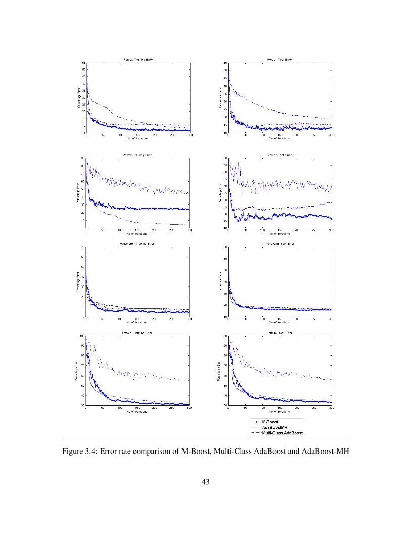
Figure 3.4: Error rate comparison of M-Boost, Multi-Class AdaBoost and AdaBoost-MH

43

Dataset Training Error Test ErrorM-Boost AdaBoost-MH Multiclass M-Boost AdaBoost-MH Multiclass

Iris 0.833 0.167 0.000 6.452 3.871 5.161

Pendigit 13.824 4.257 26.515 19.434 10.832 29.323

Forest 6.900 5.200 10.750 13.267 14.851 15.050

Glass 0.000 0.000 31.775 2.738 2.273 31.501

Vowel 24.621 1.136 37.500 46.004 54.644 67.819

Landstat 17.475 16.347 58.219 20.290 19.54 58.471

Wine 0.843 0.000 0.000 8.213 3.273 4.384

Waveform 5.000 5.000 6.330 15.848 17.103 17.018

Yeast 46.327 32.653 54.286 55.050 42.574 59.010

Letters 30.800 32.981 55.356 33.267 35.066 56.611

Segmentation 0.000 0.000 8.095 10.186 5.854 12.661

Table 3.3: Percent error rate comparison of M-Boost, AdaBoost-MH and Multi-Class AdaBoost

Figure 3.5: Number of datasets per test error interval

44

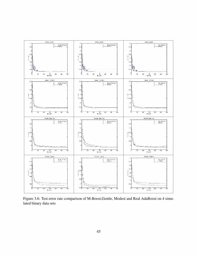
Figure 3.6: Test error rate comparison of M-Boost,Gentle, Modest and Real AdaBoost on 4 simu-lated binary data sets

45

Figure 3.7: Test error rate comparison of M-Boost, Gentle, Modest and Real AdaBoost on 3 binarydata sets from UCI repository

46

to learn a classifier for the smaller problem. At each step of our experiments the classes were

partitioned into two sets. The first set always had a single class whereas the second set consisted of

all the remaining undecided classes. For example we used the Normal class at the root followed

class labeled 19 and so on. Therefore the resulting cascade, in our experiments, has been similar

to the cascade structure shown in Figure 3.2.2

Next we present a detailed description/statistics of the dataset used in our experiments followed

by the experimental settings and results obtained from these experiments. A detailed comparison

of the proposed cascade structure with the performance of AdaBoost-M1 and that of Multiclass

AdaBoost is also provided.

Dataset Description

The dataset used in our experimental work is adopted from the KDD Cup 99 (KDD’99) dataset

prepared and managed by MIT Lincoln Labs as part of the 1998 DARPA Intrusion Detection

Evaluation Program. KDD’99 was first used for the 3rd International Knowledge Discovery and

Data Mining Tools Competition in 1999. Since then, KDD’99 has became a dominant intrusion

detection dataset which has been widely used by most researchers to evaluate and benchmark their

work related to various types of intrusion detection [3, 4, 11, 30, 55].

The dataset consists of processed TCP dump portions of normal and attack connections to a

local area network simulating a military network environment. There are 23 different types of

attack instances in the dataset falling into four main categories, namely: denial of service (DoS)

such as syn flood, unauthorized access from a remote machine (R2L) such as password guess,

unauthorized access to local root privileges (U2R) such as rootkit, and probing such as port scan

and nmap. The adopted dataset has 494021 connections; each described using 41 attributes and

a label identifying the type of connection (either normal or one of the attacks). Two attributes

are symbolic whereas the remaining 39 attributes are numeric. The attributes are divided into

four groups: basic attributes of individual connections (9 attributes), content attributes within a

47

connection suggested by domain knowledge (13 attributes), time-based traffic attributes computed

using a two-second time window (9 attributes), and host-based traffic attributes computed using

a window of 100 connections to the same host (10 attributes). A summary of the attributes is

provided in Tables 3.4 3.5. Detailed statistics and a percentage split of examples belonging to

various classes are shown in Figure 3.8. It is clear from these statistics that the dataset has three

dominant classes covering more than 98% of the total examples. This dominance of few classes

poses a very interesting learning problem as many of the learning algorithms, in an effort to attain

high accuracy, tend to ignore most of the smaller classes and hence attain very poor accuracy on

the classes.

(a) (b)

Figure 3.8: Dataset Statistics

In our first set of experiments 10-fold cross validation has been used to estimate the test error

rate the cascade and that of AdaBoost-M1 and Multiclass AdaBoost. The dataset has been ran-

domized and split into 10 non-overlapping partitions and the training and testing are repeated 10

times using a different partition for testing and the remaining partitions for training. In these exper-

iments, decision stumps have been used as the base classifiers in all the boosting based algorithms.

The reason for using decision stumps is that a domain partitioning algorithm like decision stump

can be easily modified to output class probabilities instead of a class predictions. To estimate the

48

Table 3.4: Dataset Summary: Category, Notation, Name, Type, Statistics and Description

StatisticsNot. Name Type Min Max Description

Basic Category Attributesa1 duration num. 0 58329 Connection length in secondsa2 pro_type cat. – – Prototype type which can be tcp, udp, or icmp.a3 srv cat. – – Service on the destination; there are 67 potential

values such as http, ftp, telnet, domain, etc.a4 flag cat. – – Normal or error status of the connection; there

are 11 potential values, e.g. rej, sh, etc.a5 src_bytes num. 0 693M Num. of bytes from the source to the destina-

tiona6 dst_bytes num. 0 52M Num. of bytes from the destination to the

sourcea7 land binary – – Whether conn. from/to same host/port or nota8 wrng_frg num. 0 3 Number of wrong fragmentsa9 urg num. 0 3 Number of urgent packets

Content Category Attributesa10 hot num. 0 30 Number of hot indicatorsa11 n_failed_lgns num. 0 5 Number of failed login attemptsa12 logged_in binary – – Whether successfully logged in or nota13 n_cmprmsd num. 0 884 Number of compromised conditionsa14 rt_shell binary – – Whether root shell is obtained or nota15 su_attmptd num. 0 2 Number of “su root” commands attempteda16 n_rt num. 0 993 Number of accesses to the roota17 n_file_crte num. 0 28 Number of create-file operationsa18 n_shells num. 0 2 Number of shell promptsa19 n_access_filesnum. 0 8 Number of operations on access control filesa20 n_obnd_cmds num. 0 0 Number of outbound commands in an ftp ses-

siona21 is_hot_lgn binary – – Whether login belongs to hot list or nota22 is_guest_lgn binary – – Whether guest login or not

49

Table 3.5: Dataset Summary: Category, Notation, Name, Type, Statistics and Description

StatisticsNot. Name Type Min Max Description

t_traffic (using a window of 2 seconds)a23 cnt num. 0 511 Number of same-host connections as the cur-

rent connection in the past 2 secondsa24 srv_cnt num. 0 511 Num. of same-host conn. to the same service as

the current connection in the past 2 secondsa25 syn_err num. 0 1 Percentage of same-host conn. with syn errorsa26 srv_syn_err num. 0 1 Percentage of same-service conn. with syn er-

rorsa27 rej_err num. 0 1 Percentage of same-host conn. with rej errorsa28 srv_rej_err num. 0 1 Percentage of same-service conn. with rej er-

rorsa29 sm_srv_r num. 0 1 Percentage of same-host conn. to same servicea30 dff_srv_r num. 0 1 Percentage of same-host conn. to different ser-

vicesa31 srv_dff_hst_r num. 0 1 Percentage of same-service conn. to different

hostsh_traffic (using a window of 100 connections)

a32 h_cnt num. 0 255 Number of same-host connections as the cur-rent connection in the past 100 connections

a33 h_srv_cnt num. 0 255 Num. of same-host conn. to the same service asthe current connection in the past 100 connec-tions

a34 h_sm_srv_r num. 0 1 Percentage of same-host conn.to same servicea35 h_dff_srv_r num. 0 1 Percentage of same-host conn. to different ser-

vicesa36 h_sm_sr_prt_rnum. 0 1 Percentage of same-service conn. to different

hostsa37 h_srv_dff_hst_rnum. 0 1 Percentage of same-service conn. to different

hostsa38 h_syn_err

num.0 1 Percentage of same-host conn. with syn errors

a39 h_srv_syn_errnum. 0 1 Percentage of same-service conn. with syn er-rors

a40 h_rej_err num. 0 1 Percentage of same-host conn. with rej errorsa41 h_srv_rej_err num. 0 1 Percentage of same-service conn. with rej er-

rors

50

conditional probability p(cj|x) for a given partition, the weight Wj of class j instances and the

total weight W of all instances in the partition are used to compute the class probability using:

p(cj|x) =Wj + β

W + k.β(3.8)

The constant β in the above equation acts as a small smoothing value that is used to avoid zero

probabilities.

The first set of results, shown in Table 3.6, give a weighted average of four commonly used

performance measures including Accuracy, Precision, Recall and F-Measure. It is clear that all

learning algorithms in general and the M-Boost based cascade in particular attained very high

average values for all the four performance measures.

In our second set of experiment, similar results have been obtained using a straight split of the

dataset into a training set and a test set. In these experiments we used 3.4% data for training the

classifiers and the remaining 96.6% data has been used as test set. The second set of results, shown

in Table 3.7, give a weighted average of Accuracy, Precision, Recall and F-Measure. These results

are quite similar to the first set of results with the M-Boost based cascade and Multiclass AdaBoost

giving better average results than those of AdaBoost-M1.

3.4 Summary

This chapter presented our two new methods of creating classifier ensembles to handle multiclass

learning problems. First of these methods, M-Boost, is a boosting like algorithm that creates a

multiclass ensemble without dividing the problem into several binary classification problems. The

second method, CBC, divides a given multiclass learning problem into several multiclass learning

problems by partitioning the classes and use a divide-and-conquer strategy to learn a multiclass

classifier.

51

Table 3.6: Comparison of various methods in terms of accuracy, precision, recall and F1 measurefor training and testing

Phase Method Accuracy Precision Recall F1 MeasureTraining

AdaBoost-M1 0.991±0.0004 0.964±0.0003 0.973± 0.005 0.96± 0.007Multiclass Ad-aBoost

0.999±0.0001 0.998±0.0003 0.998± 0.003 0.997± 0.008

Cascaded M-Boost

1± 0.0001 0.999±0.0001 0.999±0.0013 0.999± 0.002

TestingAdaBoost-M1 0.989± 0.001 0.957± 0.004 0.964± 0.004 0.961± 0.006Multiclass Ad-aBoost

0.998± 0.006 0.997± 0.004 0.997± 0.005 0.996± 0.007

Cascaded M-Boost

0.999±0.0001 0.998±0.0003 0.999± 0.003 0.998± 0.003

Table 3.7: Comparison of various methods in terms of accuracy, precision, recall and F1 measurefor training and testing

Phase Method Accuracy Precision Recall F1 MeasureTraining

AdaBoost-M1 0.994 0.961 0.978 0.969Multiclass Ad-aBoost

1 0.999 0.999 0.999

Cascaded M-Boost

1 0.999 0.999 0.999

TestingAdaBoost-M1 0.994 0.962 0.978 0.970Multiclass Ad-aBoost

0.999 0.999 0.999 0.999

Cascaded M-Boost

0.999 0.999 0.999 0.999

52

M-Boost introduces a new classifier selection and classifier combining rules and uses deci-

sion stumps as base classifier to handle a multi-class problem without breaking it into multiple

binary classification problems. M-Boost uses a global optimality measures for selecting a weak

learner as compared to standard AdaBoost variants that use a localized greedy approach. It uses a

reweighing strategy for assigning weights to training examples as opposed to standard exponential

multiplicative factor used to modify training example weights. M-Boost uses a probabilistic base

learner outputs a probability distribution over all classes rather than a binary classification deci-

sion. The chapter also presented an experimental setup to compare M-Boost with AdaBoost-M1

and Multi-class AdaBoost.

The chapter also presented a novel encoding based approach of creating a multi-class cascade

of classifiers called CBC. The method used in CBC does not require explicit encoding of the given

multiclass problem, rather it learns a multi-split decision tree and implicitly learns the encoding

as well. In this recursive approach, an optimal partition of all classes is selected from the set of

all possible partitions of classes, the training data is relabeled, and the reduced multiclass learning

problem is learned through applying any multiclass algorithm. The proposed method has been

used to build a multi-class cascade to classify instances belonging to one of the 43 classes in a

benchmark network intrusion dataset adopted from the KDD Cup 99 dataset.

53

Chapter 4

Incorporating Prior into Boosting

Machine learning literature discuss, in detail, several effective methods of creating a classifier

from a given set of labeled training examples {(xi, yi)|i = 1, 2, . . . , N}. However, most of the

real world learning problems have significant prior knowledge that might be used along with the

training data to optimize the learned classifier. Such prior might be available in the form of very

simple rules, like an audio frame with very low average energy is highly unlikely to have any

voice activity of interest or the part of the image without any edges is highly unlikely to contain

a human face, or it can be available in the form of a probability distribution function that can

be used to predict probabilities of various events. In general, the features designed to train an

optimal classifier are discriminative and their values are a good indicator of the actual class of an

instance. Such knowledge or information about the structure of an instance space can either be

provided by a human expert or can be efficiently generated from the labeled training data itself.

Problem however remains as to how this domain knowledge be effectively incorporated into a given

learning algorithm. This chapter presents a method of incorporating prior effectively into boosting

based ensemble learning algorithms. The method, called AdaBoost-P1, uses a hypotheses space

of probabilistic classifiers and introduces a novel method of classifier selection so that the prior is

incorporated into ensemble learning.

54

In the rest of the chapter, a short review of various methods of incorporating prior into classifier

learning algorithms and the discussion of an existing method of incorporating prior into AdaBoost

is presented in Section 4.1. Section 4.2 describe, in detail, the proposed method of incorporat-

ing prior into boosting based ensembles and the experimental settings and corresponding results

obtained are presented in Section 4.3.

4.1 Introduction

In the supervised learning setting a learning method is presented with a set of labeled training

examples and is assumed to generate a model that can be used to label future instances. Most

of the supervised learning literature, therefore, presents methods to learn a classifier from the

training data alone [33, 28, 71, 16, 61, 58, 90]. However, several real world learning problems have

significant domain/prior knowledge available about the problem structure along with the training

data. For example the presence or absence of a key word might be a good indicator of a documents

actual class. Further, the feature space representation of a problem is generally very expressive as

the computed features typically discriminate a class from other classes. Such domain knowledge

or information about the structure of instance space can either be provided by a human expert or

generated automatically from the training data itself.

Machine learning literature presents several useful methods of incorporating prior knowledge

into various classifier learning algorithms including SVM, Naïve Bayes, decision tree learning

etc [64, 86, 99, 54, 102, 57]. Niyogi et. al. [64] suggested a general framework of using prior

knowledge to generate additional virtual training examples and hence prior is used to address the

problem of training data sparsity. Schölkopf and Simard [86] uses an appropriate kernel function to

incorporate prior into SVM classifiers. Another method of incorporating prior into SVM has been

proposed by Wu and Srihari [99] that uses the idea of assigning weights to training examples using

prior knowledge and then computes an optimal separating hyperplane using the weighted margins.

55

Krupka and Tishby [54] uses a feature based prior to define a vector of meta-features and uses

these meta-features to incorporate prior into learning a SVM . Zhu and Chen [102] used domain

specific information for document classification whereas Liu et. al [57] used the prior along with

Naïve Bayes classifier to create a text classifier.

The use of prior knowledge along with different types of classifier learning algorithms has

been an active research area in machine learning. However, the existing literature does not present

effective ways of incorporating prior knowledge into ensemble learning methods except for the

study presented by Schapire et. al. [82]. The main focus of this study is incorporation of prior into

boosting based ensemble learning algorithms and therefore the remaining discussion will primarily

address the problem of incorporating prior into AdaBoost variants.

The method presented in [82] has been introduced for learning problems suffering from the

scarcity of training data and hence incorporates prior into AdaBoost by introducing additional

virtual training examples by using prior. Empirical evidence suggest that the method described in

[82] does not present any significant advantage as the number of training examples increase. That

means, their method does not use the domain knowledge for a faster convergence or for obtaining

better accuracy when sufficient amount of training data is already available. Ideally one would

expect the domain knowledge to compensate the lack of training data for problems suffering from

scarcity of data, and on the other hand help in reducing the convergence time and/or improve

overall accuracy if the training data is in abundance. Moreover, the method presented in [82]

does not generalize to all boosting algorithms and uses only one specific variant of AdaBoost to

incorporate prior into boosting. In summary the existing method of incorporating prior knowledge

into boosting has the following shortcomings

• The method becomes ineffective in terms of prediction accuracy and inefficient when large

training set is already available.

• The method is limited to only one boosting algorithm and can not be generalized to a wide

56

verity of boosting algorithms.

To address these issues, a novel method of incorporating prior into boosting is presented in this

chapter that improves the overall classification accuracy, compensates for lack of training data,

and improves the convergence rate of boosting algorithms. Moreover, the proposed method is not

specific to a single boosting algorithm and can be used to incorporate prior into a large class of

boosting algorithms. The proposed method, therefore, covers the aforementioned limitations of

the state-of-the-art method of incorporating prior into boosting.

The proposed method uses prior to modify the weight distribution maintained over training

examples and hence effects the selection of base classifier in each boosting iteration. Further it

also uses the prior as a component classifier and as a multiplicative factor in the overall ensemble

and hence incorporates the available prior into ensemble learning. The method works for domain

knowledge of varying quality i.e., for situations when the domain knowledge is relatively precise to

situations when it is vague. While the method of Schapire et. al [82] is based on only one specific

variant of AdaBoost algorithm, our method can be used to incorporate prior into any boosting

algorithm that can handle a probabilistic base classifier ht. Such classifiers output a conditional

density over classes for an input instance x. Learning algorithms like decision trees, stumps and

classifiers that output confidence rated predictions can be readily modified to output the required

class conditional density instead of the classification decision [84] and hence can be used with the

proposed method. The proposed method has been applied to several synthetic and real datasets

of varying complexity with stumps as base classifier. In several cases, significant improvement in

classification accuracy has been observed. The use of prior also resulted in faster convergence of

boosting algorithms and hence improved efficiency of the learned ensemble. The proposed method

has been further extended to handle two different cases of a real valued base learners i) when the

base learners output a bounded signed output and ii) for the case when a bounded unsigned outputs

are produced by the base learner.

57

4.2 Incorporating Prior into Boosting

To describe the proposed method of incorporating prior knowledge into any boosting algorithm

that generates a probabilistic classifier, we initially consider a binary classification problem. A

straight forward extension to handle multiclass learning problems is described later. The descrip-

tion assumes that that the boosting algorithm is provided with a set of n labeled training examples

{(xi, yi)|i = 1 . . . n} where yi ∈ {+1,−1}. Further, the probabilistic classifierH generated by the

boosting algorithm outputs estimates of class conditional density f(y+|x) denoting the probability

of y being +1 given x. Like the method of Schapire [82], It is also assumed that the prior has been

provided in the form of a conditional density π(y+|x) denoting the probability of y being +1 given

x.

As described by Coryn A.L [20], there are two equivalent ways to combine the estimates of

class probabilities obtained from two independent different sources to get a single estimate of

class probabilities. The first method of combining the probabilities uses an averaging procedure

to get an overall estimate of class probabilities whereas the second method uses a multiplicative

method to combine class probabilities obtained from two different sources. These two methods

are equivalent in the sense that both these approaches result into equivalent classifiers. To combine

the class probability estimates obtained from the prior, F (x) = π(y+/x), and from the output

of ensemble, H(x), we take the second approach. Therefore, a combined estimate of probability

P (y+|x) can be computed using the product of these two probability estimates as

P (y+/x) = βπ(y+/x).f(y+/x) (4.1)

where β is a normalization constant.

AdaBoost like most boosting based algorithms compute a linear combination of selected clas-

58

sifiers to build the final ensemble so the final form of ensemble produced by boosting is

f(y+/x) =T∑t=1

αt.ht(x) (4.2)

Substituting 4.2 into 4.1 we obtain

P (y+/x) = δ.π(y+/x).T∑t=1

αt.ht(x) (4.3)

where δ is a normalization constant.

Equation 4.3 is our main equation for incorporating prior knowledge into boosting algorithm when

the boosted classifier output density estimates over the possible classes. The resulting boosting

algorithm works exactly like AdaBoost except that the final classifier is formed as

H(x) = sign

(log

(P (y+/x)

1− P (y+/x)

))(4.4)

This equation can be used with any base classifier that output class density estimate. In case of

base classifiers that produce binary or confidence rated output the value of each ht(x) must be

converted into probability estimates, for example by using logistic regression function, and then

the product similar to equation 4.3 can be computed. When each base classifier ht output class

conditional density, equation 4.3 can be written as

P (y+/x) =T∑t=1

αt.π(y+/x).ht(x) (4.5)

Equation 4.5 is used to derive our method of incorporating prior into any boosting algorithm that

uses probabilistic base learner. From this equation it is obvious that

To incorporate prior into boosting we consider prior combined base classifiers of the form

pt(x) = π(y+/x).ht(x) instead of ht(x). Therefore, in each boosting iteration a classifier instance

59

pt(x) = π(y+/x).ht(x) that gives optimal performancew.r.t the weight distributionDt is selected.

It is important to note that a direct selection of such a pt(x) requires modification in the base learn-

ing algorithm so that both the prior, π(y+/x), and the weight distribution,Dt, are used for selecting

a classifier ht. Such a modification is feasible only when a very simple learning algorithms like

decision stump is used as base learner but for most of learning algorithms, e.g. Decision Trees,

Support Vector Machines, Neural Networks, e.t.c., such a change is not obvious or not feasible due

to exponentially many classifiers to search from.

We, therefore, take a two step approach to use prior for selecting an optimal classifier pt(x)

w.r.t Dt. In the first step, prior is used to modify the weight distribution maintained on training

examples followed by the second step of selecting the classifier instance ht using the modified

weight distribution. Weight distribution is modified so that weights of examples misclassified

by the prior are increased by an exponential multiplicative factor. This multiplicative factor is

computed exactly like the multiplicative factor computed in each boosting iteration. Calculation of

the weight modifying factor is based on the error rate, εp, of the priorw.r.t. the running distribution

Dt. The modified distribution is normalized and used to select the classifier instance ht using the

base learning algorithm without any modification. Therefore, the prior affects the selection of

base classifier via the weight modification step. In each boosting iteration, this two step process

mimics fitting a combination of two classifiers, first the fixed prior π(y+|x) followed by the fitting

a classifier instance ht using the learning algorithm. Following the method of Schapire [82] the

prior is added as a component classifier, h0 in the final ensemble. The weight α0 of h0 is set equal

to 1− ε0 where ε0 is the error rate of h0 on the training data.

The boosting algorithm, AdaBoost-P1 that results from incorporating prior into learning is

given as Algorithm 5. The algorithm takes as inputs n labeled training examples (x1, y1) . . . (xn, yn),

a parameter T specifying the total base classifier instances to be used for ensemble construction and

the prior π(y+/x) giving the probability of an instance x being in class +1. The algorithm main-

tains a running distribution Dt on training examples which is initially uniform. In each boosting

60

Algorithm 5 : AdaBoost-P1

Require: Examples (x1, y1) . . . (xn, yn) wherexi is a training instance and yi ∈ {−1,+1} andparameter T = total base learners in the ensembleπ(y+/x) : Domain knowledge in the form of Prior

1: set D1(i) = 1n

for i = 1 . . . n

2: for t =1 to T do3: Compute labels ypi = sign

(log( π(y+|xi)

1−π(y+|xi)))

4: set εp = Pr[ypi 6= yi] w.r.t Dt

5: set αp = 12log(1−εp

εp)

6: Set Dtemp(i) = Dt(i). exp(−αp.yi.ypi )7: Normalize the weight distribution Dtemp(i)

8: Select a weak classifier instance ht which has small error w.r.t Dtmp

9: Compute labels Opi = sign

(log( π(y+|xi).ht(xi)

1−π(y+|xi).ht(xi)))

10: set εt = Pr[Opi 6= yi] w.r.t Dt

11: set αt = 12log(1−εt

εt)

12: Set Dt+1(i) = Dt(i) exp(−αt.yi.Opi )

13: Set Dt+1(i) = Dt+1(i)Zt

where Zt is the normalization factor14: end for15: output classifier

H(x) =∑T

t=0 αt.ht(x)∑Tt=0 αt

.π(y+/x)

class with maximum probability estimate is the predicted class.

61

iteration, the prior is used to predict the labels of training examples and an intermediate distribu-

tion Dtmp is computed using the error rate of the prior π(y+/x) w.r.t. the Dt. This intermediate

distribution is then used to select a classifier instance ht. An example misclassified by prior get

larger weight than its’ weight in Dt and hence the prior affects the selection of the base classifier

ht. Finally, a weight distribution is updated toDt+1 using the error rate of prior combined classifier

pt(x) = π(y+/x).ht(x) instead of the error of ht alone.

Multiclass Extension

AdaBoost-P1 can be naturally extended to handle multiclass learning without a major modification.

To incorporate prior into multiclass the prior must be provided in the form of a conditional density

π(y/x) denoting the probability of label being y given x. The label y in this case comes from a

larger set {y1, y2, . . . , yk} for a k-class learning problem. Like the binary classification problem it

is assumed that the base learning algorithm output a classifier ht that gives the estimate of class

conditional density f(y|x). With these changes equation 4.5 becomes

P (y/x) =T∑t=1

αt.π(y/x).ht(x) (4.6)

So our method of incorporating prior remains the same with the product, π(y/x).ht(x), being a

normalized point by point product of two densities.

4.2.1 Generating the Prior Knowledge

Schapire [82] suggested a process to construct prior knowledge for the text categorization datasets.

His method requires the domain experts to associate various keywords to titles or categories. The

probability of a particular topic/dialogue is then computed by assuming independence of occur-

rence of the keywords and taking product of probabilities obtained from the presence or absence of

various keywords in a given article. In general their technique works well for problems involving

62

categorical features. To adapt this technique for features having continuous values we require that

the experts provide us a sequence of threshold values and corresponding values of class probabili-

ties for each partition of feature values defined by the threshold values. The class probabilities so

obtained must be multiplied and normalized to obtain the final estimate of class probabilities.

A difficulty associated with the above techniques of generating prior from expert opinion is

that it requires a human experts to assign the probabilities. To overcome this difficulty we suggest

an automatic way to construct prior knowledge using the structure of the instance space. In our

approach we compute a model, Gaussian in our case, for each class and use that model to assign

the prior probabilities. The parameters of the model are computed using maximum likelihood

estimates as is done in the naive Baye’s approach. Therefore, our method involves the training data

to estimate the prior and hence captures the structure of instance space. It is important to note that

such a prior can not be called a prior in the true statistical sense even though such probabilities are,

often, very accurate. Since our method of incorporating prior only assume that the prior has been

provided in the form of a class conditional density so output of any previously learned confidence

rated or probabilistic classifier can also be used as prior in our method without much modification.


Several experiments have been performed to study the effects of using the proposed method of

incorporating prior into boosting. The results reported in this paper compare the performance of

two boosting algorithms AdaBoost-M1 [33] and Multiclass AdaBoost [103] with and without

incorporating prior.

Decision tree learning has been used as base algorithm with the results reported for decision

stumps (i.e. single node decision trees) and dlog(K)e split decision trees for a K class learning

problem. A decision stump partitions the instance space into two parts where as a dlog(K)e split

decision tree partitions the instance space into a maximum of 2dlog(K)e = K parts. The class prob-

63

ability estimates, to be used in the proposed method, have been obtained by using the frequency

counts of each class instances falling in a given partition determined by the decision tree. To avoid

a probability estimate of 0, all zero class counts were replaced with a small number ε representing

a small class probability. A set of 200 base classifiers has been used to build the final ensemble

with this number selected empirically as it gives a fair idea of both the training and test error rates.

Experimental results on twelve multiclass learning problems and four binary classification

datasets mostly from the UCI machine learning repository [56] are presented in this paper. These

learning problems include three simulated binary classification problems the two-norm, three-norm

and ring-norm taken from the work of Leo Breiman [16]. The main characteristics of all the

datasets including the dimension of instance space, training set and test set sizes and the number of

classes are summarized in Table 4.1. Both synthetic and real world multiclass learning problems

of varying complexity are included in these datasets.

To get an estimate of test error rate, 10-Fold cross validation has been used for datasets without

explicit division into training and test sets and a paired t-test, as reported by Dietterich [24], has

been used to compare the boosting algorithms with and without incorporating prior in this case. In

case of 10-fold cross validation a value greater than 1.82 indicates a significant difference between

the performance of two algorithms.

For the datasets with explicit training and test set division, the complete training set has been

used to learn the ensemble and the given test set used to estimate the test error. The test for

difference of proportions has been used as described by [89] has been used in this case to compare

the boosting algorithms with and without incorporating prior. A z-score of more than 1.96 indicates

a significant difference between the performance of two algorithm with 95% confidence.

The first set of experiments compare the performance of the two boosting algorithms with and

without incorporating the prior. In the first experiment, a single node decision tree has been used as

the base classifier where as in the second experiment a stronger decision tree classifier with log(K)

splits has been used as the base classifier. The prior in these experiments have been obtained using

64

our method of generating prior as described in section 4.2.1.

A second set of experiment studies the effect of prior quality when the prior is changed from

perfect prior to uniform prior and then to poor prior. A prior is considered perfect if it mostly

assigns a high probability (i.e. ≈ 1) to the actual class and a prior is poor if it assigns a low

probability (i.e. < 1K

) to the actual class for most instances.

Finally the last experiment demonstrate the use of prior to compensate the sparsity of training

data. The prior, in this experiment, is fixed and the amount of training data is varied from 1% to

100%.

4.3.1 Results and Discussion

The First set of results presents a comparison of Multiclass AdaBoost [103] and AdaBoost-P1.

These experiments have been carried out both with multi-split decision tree {Log(K) splits} and

with decision stumps as base learning algorithm.

Table 4.2 compares the test error rate of Multiclass AdaBoost algorithm with and without incor-

porating prior knowledge for datasets having distinct training and test sets. The prior knowledge

in all these experiments have been obtained from the training data itself and was slightly, (0.15%),

biased towards the actual class. The first three dataset are simulated binary classification problems

whereas the remaining datasets are multiclass problems involving 3 to 25 classes. The table lists

the test error rates of the two algorithms along with the z-score indicating the significance of dif-

ference between two algorithms. As mentioned previously, a value of z-score greater than 1.96

indicates a significant difference between the two algorithms with a high confidence value.

For both cases, multi-split decision trees or decision stump as base classifiers, the effect of in-

corporating prior has been significantly positive and the algorithm with incorporating prior knowl-

edge converged to a better ensemble than the algorithms without it. In case of the simulated ring-

norm dataset the proposed method of incorporating prior had a negative impact on the algorithm

performance.

65

Table 4.1: Datasets Used in Our Experiments.

DATA SET TOTAL TRAINING TEST TOTAL

NAME FEATURE SET SET CLASSES

TWO NORM 20 2000 1000 2THREE NORM 20 2000 2000 2RING NORM 20 2000 2000 2WISCONSIN BREAST CANCER 4 569 — 2SPAMBASE 57 4601 — 2IRIS 4 150 — 3FOREST FIRE 4 500 — 4GLASS 10 214 — 7WINE 13 214 — 3PEN DIGIT 16 7494 3498 10VOWEL 10 528 462 11LAND STATE 36 4435 2000 8WAVEFORM 21 300 4710 3YEAST 8 980 504 10ABALONE 8 3133 1044 29LETTERS 16 16000 4000 26SEGMENTATION 19 210 2100 8

Table 4.2: Test Error rate Comparison of Multiclass AdaBoost and AdaBoost-P1

MULTI-SPLIT DECISION TREES DECISION STUMPS

DATA SETNAME

TWO NORMTHREE NORMRING NORMPEN DIGITVOWELLAND STATEWAVEFORMYEASTABALONELETTERSSEGMENTATION

MULTICLASS ADABOOST Z-SCOREADABOOST P1

3.45 1.45 4.0918.24 12.24 5.27

2.99 49.69 37.054.23 1.83 5.85

59.83 26.78 10.1338.08 0.80 29.7315.02 3.69 11.1754.05 8.71 15.5174.73 1.15 34.6417.69 0.0 27.86

6.13 2.0 6.71

MULTICLASS ADABOOST Z-SCOREADABOOST P1

3.45 1.45 4.0918.24 12.24 5.27

2.99 49.69 37.0529.32 0.43 33.9571.49 0.22 22.5849.48 0.2 36.0613.99 3.94 10.1065.74 0.79 21.8882.30 1.24 37.5561.03 0.0 59.2711.23 1.43 13.05

Table 4.3: Test Error rate Comparison of Multiclass AdaBoost and AdaBoost-P1


DATA SETNAME

SPAMBASEIRISFOREST FIREGLASSWINE

MULTICLASS ADABOOST PAIREDADABOOST P1 T-TEST

4.48 7.71 9.486.25 5.25 0.94

11.80 5.0 2.5430.43 0.9 2.86

2.76 2.3 0.23

MULTICLASS ADABOOST PAIREDADABOOST P1 T-TEST

4.48 7.71 9.484.7 3.42 1.51

13.73 3.92 2.9110.43 9.7 1.21

6.11 1.26 2.55

66

For datasets without a clear partitioning into training and test sets, a comparison of Multiclass

AdaBoost with and without incorporating prior knowledge is given in Table 4.3. For these learning

tasks we used 10-fold cross validation to estimate the test accuracy of the learning algorithm and

hence the paired t-test has been used to compare the algorithms. A test value greater than 1.84,

in this case, indicates significantly different performance of the two algorithms. Performance of

Multiclass AdaBoost is better than AdaBoost-P1 {Multiclass AdaBoost with prior} only in case

of the spambase binary classification dataset whereas AdaBoost-P1 outperformed the Multiclass

AdaBoost for the remaining datasets.

Contrary to the intuition, it has also been observed that the impact of prior has been much

more significant in case of the decision stumps than in case of the multi-split decision trees. This

effect can be attributed to the peaky estimates of class probabilities in case of decision trees in

comparison of decision stumps. It can also be observed that the difference in performance of

algorithms is more significant in case of larger number of classes as the algorithm without prior

"mostly" giving a poor performance for such learning problems.

Another important aspect of these results is highlighted in Figure 4.1. These plots show the

test error vs. number of boosting iterations for Multiclass AdaBoost and AdaBoost-P1. Except for

the ring-norm dataset the convergence of AdaBoost-P1 required fewer iterations.

Tables 4.4 and 4.5 present a comparison of AdaBoost-M1 for dataset having different training

and test sets. AdaBoost-M1 performs extremely well only if the accuracy of base classifier is better

than 50% and it diverges otherwise. For most of the datasets used in our experiments the algorithm

diverged as the base classifiers had error rate greater than 50%. The impact of using a probabilistic

base classifiers along with the proposed method of incorporating prior into AdaBoost-M1 has been

huge both when a decision stump or multi-split decision trees are used as base classifiers. The

rate of convergence of the AdaBoost-M1 and AdaBoost-P1 is shown in Figure 4.2. The unusual

error rates of AdaBoost-M1 are due to the fact that a naive classifier such as a decision stump

mostly failed to grantee an accuracy greater than 50% whenever the number of classes is large.

67

0 50 100 150 2000

0.05

0.1

0.15

0.2

0.25

0.3

0.35

No of Iterations

% E

rror

Two Norm

Without PriorAdaBoost−P1

0 50 100 150 2000.1

0.15

0.2

0.25

0.3

0.35

0.4

0.45

0.5

No of Iterations%

Err

or

Three Norm


0 50 100 150 2000

0.1

0.2

0.3

0.4

0.5

0.6

0.7

No of Iterations

% E

rror

Ringnorm


0 50 100 150 2000.04

0.06

0.08

0.1

0.12

0.14

0.16

0.18

0.2

0.22UCI: Spambase

No of Iterations

% E

rror

0 50 100 150 2000

0.1

0.2

0.3

0.4

0.5

0.6

0.7

No of Iterations

% E

rror

PenDigit


0 50 100 150 2000

0.05

0.1

0.15

0.2

0.25

0.3

0.35

0.4

0.45

0.5Forest Fire

No of Iterations

% E

rror

0 50 100 150 2000.2

0.3

0.4

0.5

0.6

0.7

0.8

0.9

1

No of Iterations

% E

rror

Vowel Recognition


0 50 100 150 2000

0.05

0.1

0.15

0.2

0.25

0.3

0.35

0.4

0.45

No of Iterations

% E

rror

Land Stat


0 50 100 150 2000

0.05

0.1

0.15

0.2

0.25

0.3

0.35

0.4

No of Iterations

% E

rror

Waveform


0 50 100 150 2000

0.1

0.2

0.3

0.4

0.5

0.6

0.7

0.8

No of Iterations

% E

rror

Yeast


0 50 100 150 2000

0.1

0.2

0.3

0.4

0.5

0.6

0.7

0.8

0.9

No of Iterations

% E

rror

Abalone


0 50 100 150 2000

0.1

0.2

0.3

0.4

0.5

0.6

0.7

0.8

No of Iterations

% E

rror

Letters


Figure 4.1: Test Error: AdaBoost-P1 vs Multiclass AdaBoost

68

The weight of the selected classifiers computed at step 5 of Algorithm 1 using αt = 12log(

1−εtεt

)becomes negative in such a case and the algorithm diverges. Such behaviour of AdaBoost-M1 is

well known and has already been reported in literature [103].

Table 4.6 presents the result of our second set of experiment that studies the effect of prior qual-

ity on the convergence of Multiclass AdaBoost. log(k)-split decision trees have been used in these

experiments and the prior is changed from negatively-biased (prior that assigns low probability to

actual class) to perfect prior (Prior that assigns high probability to actual class).

Figure 4.3 presents the results of our last experiment that studies the effect of prior if data is

sparse. This experiment has been repeated for the two larger datasets with training data sampled

uniformly to create new training set. For these experiment the prior was fixed in the beginning and

the experiment has been repeated with training dataset of sizes 1%, 5%, 10%, 20%, 50% and 100%

of the original training data. The figure shows the test error of AdaBoost-P1 vs. the proportion of

training data used.

4.4 Summary

This chapter described an effective method of incorporating prior knowledge into AdaBoost based

ensemble learning algorithms. The idea behind incorporating the prior into boosting in our ap-

Table 4.4: Test Error rate Comparison of AdaBoost-M1 and AdaBoost-P1


DATA SETNAME

TWO NORMTHREE NORMRING NORMPEN DIGITVOWELLAND STATEWAVEFORMYEASTABALONELETTERSSEGMENTATION

ADABOOST ADABOOST Z-SCOREM1 P1

2.95 1.45 3.2318.39 12.24 5.39

5.62 50.68 35.4110.60 3.63 11.3163.28 42.12 6.4422.34 16.54 4.3317.81 5.03 11.5443.56 23.96 6.5899.90 44.98 28.0899.03 47.81 51.84

7.66 2.0 8.55

ADABOOST ADABOOST Z-SCOREM1 P1

2.95 1.45 3.2318.39 12.24 5.39

5.62 50.68 35.4199.17 18.98 68.295.46 34.34 19.599.95 18.74 52.520.23 9.69 8.560.99 26.93 19.999.90 34.45 31.899.15 17.02 74.499.95 1.43 63.8

69

0 50 100 150 2000

0.05

0.1

0.15

0.2

0.25

0.3

0.35

No of Iterations

% E

rror

Two Norm


0 50 100 150 2000.1

0.15

0.2

0.25

0.3

0.35

0.4

0.45

0.5

No of Iterations

% E

rror

Three Norm


0 50 100 150 2000

0.1

0.2

0.3

0.4

0.5

0.6

0.7

No of Iterations

% E

rror

Ringnorm


0 50 100 150 2000.06

0.08

0.1

0.12

0.14

0.16

0.18

0.2

0.22

No of Iterations

% E

rror

UCI: Spambase


0 50 100 150 2000

0.05

0.1

0.15

0.2

0.25

0.3

0.35

No of Iterations

% E

rror

PenDigit


0 50 100 150 2000.1

0.15

0.2

0.25

0.3

0.35

0.4

0.45

0.5

No of Iterations%

Err

or

Forest Fire


0 50 100 150 2000

0.02

0.04

0.06

0.08

0.1

0.12

0.14

No of Iterations

% E

rror

Glass


0 50 100 150 2000.4

0.45

0.5

0.55

0.6

0.65

No of Iterations

% E

rror

Vowel Recognition


0 50 100 150 2000.16

0.17

0.18

0.19

0.2

0.21

0.22

0.23

0.24

No of Iterations

% E

rror

Land Stat


0 50 100 150 2000.2

0.25

0.3

0.35

0.4

0.45

No of Iterations

% E

rror

Yeast


0 50 100 150 2000.4

0.5

0.6

0.7

0.8

0.9

1

No of Iterations

% E

rror

Abalone


0 50 100 150 200

0.4

0.5

0.6

0.7

0.8

0.9

1

No of Iterations

% E

rror

Letters


Figure 4.2: Test Error: AdaBoost-P1 vs AdaBoost-M1

70

Table 4.5: Test Error rate Comparison of AdaBoost-M1 and AdaBoost-P1


DATA SETNAME

SPAMBASEIRISFOREST FIREGLASSWINE

ADABOOST ADABOOST PAIREDM1 P1 T-TEST

6.21 7.91 2.485.23 1.25 1.71

24.45 12.73 2.832.01 1.9 0.314.26 3.20 0.44

ADABOOST ADABOOST PAIREDM1 P1 T-TEST

5.21 7.91 2.483.16 2.78 0.72

23.53 3.92 2.8430.43 34.78 0.31

5.26 0.0 0.95

Table 4.6: Effect of Prior Quality on Error rate of Multiclass AdaBoost

DATA SET NEGATIVE BIASED UNIFORM FROM DATA BIASED PERFECT

PEN DIGITS 10.37 4.23 1.83 0.13 0VOWEL 65.72 59.83 26.78 3.32 0LETTERS 58.61 17.69 0 0 0

0 20 40 60 80 1000

5

10

15Letters

Training Data Percent

Err

or

Perc

ent

0 20 40 60 80 1000

5

10

15

20

25

30

35

40

45Pen Digits

Training Data Percent

Err

or

Perc

ent

Figure 4.3: Test Error: Effect of Prior in case of Sparse Training Data

71

proach is to modify the weight distribution over training examples using the prior during each

iteration. This modification affects the selection of base classifier included in the ensemble and

hence incorporate prior in boosting.

This method mitigates several shortcomings of an existing method by [82]. The method of

incorporating prior can mitigate the necessity of large amounts of training data, and irrespective

of the size of training data it can improve the convergence rate and accuracy of the boosting algo-

rithms. The new method of incorporating prior into boosting is generic and can be used with a large

class of boosting algorithms. The chapter also presented a detailed empirical evidence of our meth-

ods’ effectiveness and show improved convergence rate, improved accuracy and compensation for

lack of training data irrespective of the size of the training datasets.

72

Chapter 5

Boosting Based ANN Learning

A novel application of boosting for learning weights in a connectionist framework is presented in

this chapter. The discussion begins with the introduction of Boostron, a boosting based percep-

tron learning algorithm, that uses AdaBoost along with a homogeneous representation of decision

stumps to learn weights of a single layer perceptron. AdaBoost minimizes an exponential cost

function [35] instead of the mean squared error minimized by perceptron learning algorithm hence

it learns a different decision boundary for a given training set. Perceptrons trained using Boostron

have shown improved performance over several standard classification tasks of varying complexity.

A major limitation of the Boostron is it’s inability to learn a perceptron having hidden lay-

ers of neurons. To overcome this shortcoming, an extension of Boostron is presented that can be

used to learn a general linear, feed-forward artificial neural network (ANN) with a single hidden

layer and a single output neuron. The proposed method use two problem reductions along with

the Boostron algorithm to learn weights of neurons in a given ANN during a layer-wise iterative

traversal of all neurons in the network. Finally the proposed method is further extended to incor-

porate non-linearity into ANN learning by extending the inputs to each hidden layer neuron. The

inputs to a neuron are extended by introducing all products of features up to a certain degree as

additional inputs and hence non-linearity is incorporated into ANN learning.

73

The chapter is organized as follows. Section 5.1 provides a short Introduction of artificial

neural networks and the associated learning algorithms. A detailed description of the three com-

ponents of our proposed method is presented Section 5.2. Details of the experimental settings and

the corresponding results are presented in Section 5.4. Finally, Section 5.5 summarizes the main

contribution of the chapter and highlights some future directions.

5.1 Introduction

The single-layer Perceptron of Rosenblatt [72], as shown in Figure 5.1, is a simple mathematical

model for classification of patterns. It takes a vector x = [x0, x1, x2, . . . , xm] of features as input

and computes its class by calculating a dot product of x with an internally stored weight vector,

W = [w0, w1, w2, . . . , wm]. Most commonly, the input component x0 is permanently set to -1 with

weight w0 representing the magnitude of external bias. The output of a perceptron is computed

using some non-linear activation function such as sign and can be written as:

y = sign(W .xT

)= sign

(m∑i=0

wi.xi

)(5.1)

74

(a) Single-layer Perceptron with one output (b) Single-layer Perceptron with k outputs

Figure 5.1: Typical structure of a single-layer Perceptron

In supervised learning settings, the main aim of a neural network learning algorithm is to de-

duce an optimal set of synaptic weights from the provided input-output pairs of vectors specifying

a desired functional relationship to be modeled. For a neural networks similar to a single-layer per-

ceptron (i.e inputs are directly connected to the output units) a simple learning rule that iteratively

adjusts the connection weights so as to minimize the difference between desired and obtained out-

puts works well. For example, the well-studied Perceptron learning algorithm initializes the weight

vector to zeros and greedily modifies these weights for each misclassified training example (xi, yi)

using the Perceptron learning rule:

Wnew = Wold + η.(yi − yi).xi (5.2)

where η is a pre-specified constant known as learning rate, yi is the desired output and yi is the

estimated output.

For more complicated networks consisting of several interconnected perceptrons, such as the

network shown in Figure 5.2, the weight adjustment of hidden neurons posed the main research

75

challenge. However, since the emergence of back-propagation algorithm [74] a number of different

learning algorithms have been proposed to adapt the synaptic weights [46, 69, 38, 45, 42, 47].

Typically, these methods use an iterative weight update rule to learn an optimal network structure

from the training examples by minimizing an appropriate cost function. For example, the back-

propagation algorithm [74] uses the following weight update rule to minimize a measure of mean

squared error using gradient of error function w.r.t the weights

Wnew = Wold − η.∂E(W )

∂W(5.3)

The gradients for output neurons are computed from the definition of error function whereas the

gradients for hidden neurons are computed by propagation of gradients from the output to hidden

neurons. Since its introduction, the gradient based back-propagation learning algorithm has been

extensively used to learn models for a very diverse class of learning problems [97, 101, 63]

The gradient based back-propagation algorithm and its variants have a manual parameter (η:

learning rate) to play with which is tricker to work with as for smaller values of η the converges of

the algorithm becomes very slowly whereas for larger values the algorithm might become unstable.

The problems of converging to a local minimum and over-fitting are also amongst the well-known

issues with gradient descend based learning algorithms. Although the mean-squared error mini-

mized by the gradient based algorithm is suitable for regression problems, it might not work well

for classification tasks because most of the natural measures of classification accuracy are typically

non-smooth.

AdaBoost is one of the most successful ensemble learning algorithm that iteratively selects

several classifier instances by maintaining an adaptive weight distribution over the training ex-

amples. AdaBoost forms a linear combination of selected classifier instances to create an overall

ensemble. AdaBoost based ensembles rarely over-fit a solution even if a large number of base clas-

sifier instances are used [100] and it minimizes an exponential loss function by fitting a stage-wise

76

additive model [35]. As the minimization of classification error implies an optimization of a non-

smooth, non-differentiable cost function which can be best approximated by an exponential loss

[80], AdaBoost therefore performs extremely well over a wide range of classification problems.

Motivated by these facts, we have devised an AdaBoost based learning method to learn a feed-

forward artificial neural network. This method consists of three components: i) a boosting based

perceptron learning algorithm, called Boostron [7], that learns a perceptron without a hidden layer

of neurons, ii) an extension of the basic Boostron algorithm to learn a single output feed-forward

network of linear neurons [8] and finally iii) a method of using series representation of the activa-

tion function to introduce non-linearity in the neurons.

5.2 AdaBoost Based Neural Network Learning

This section begins with a short review of AdaBoost algorithm which is followed by a detailed

description of our method, called Boostron, to transform the problem of perceptron learning into

learning a boosting-based ensemble. An extension of the this method that enables learning of a

linear, feed-forward perceptron network with a single hidden layer and a single output neuron is

then presented. This discussion is succeeded by the introduction of a series based approach that

can be used to introduce non-linearity into the artificial neural network learning.

AdaBoost algorithm shown as Algorithm 1 (Chapter 2 ) is used to construct a highly accurate

classifier ensemble from a moderately accurate learning algorithm. It takes n labeled training ex-

amples as input and iteratively selects T classifiers by modifying a weight distribution maintained

on the training examples. The final ensemble is constructed by taking a linear combination of the

selected classifiers using

H(x) = sign

(T∑t=1

αt.ht(x)

)(5.4)

where T is the number of base learner instances in the ensemble and αt is the weight of classifier

instance ht that is computed using its error w.r.t the running distribution Dt.

77

The basic AdaBoost algorithm that uses a binary base classifier has been extended by Schapire

and Singer [84] to handle confidence-rated outputs of a base classifier. They presented a different

criterion of selecting the base classifier and a new method for computing the weight of the selected

classifier by using

αt =1

2ln

(1 + rt1− rt

)(5.5)

where rt is the difference of correctly classified and incorrectly classified instance weights.

5.2.1 Boostron: Boosting Based Perceptron Learning

Single-node decision trees are commonly referred to as stumps and have been frequently used

as base classifiers in AdaBoost[84, 66]. Boostron uses homogeneous coordinates to represent a

decision stump [43] as a weight vector and compute its dot product with an instance x to compute

the output. A decision stump typically makes decision based on only one of the feature values. For

real-valued features, a stump consists of a feature index, say j, and a threshold, U , such that all

instances are partitioned into two sets using an if-then-else rule of the following form

78

if xji ≤ U then

Class = +ve/-ve

else

Class = -ve/+ve

end if

For an instance vector xi ∈ Rm the above decision stump can be converted into an equivalent

classifier by using the inner product defined on Rm. For example, in case when a +1 label is

assigned if xji ≤ U and a −1 label otherwise, we can create a classifier equivalent to the decision

stump as

s(xi) = −(w.xi

T − U)

(5.6)

In equation 5.6, all components of the weight vector w = [w1, w2, ..., wm] are 0 except one of the

components wj . The sign of s(xi) is the classification decision and its magnitude can be regarded

as the confidence of prediction. Such a classifier can be represented as a single dot product by

representing instance xi and the vector w using the homogenous coordinates.

s(xi) = W .XiT (5.7)

where the vector Xi = [x1i , x

2i , ..., x

mi , 1] is obtained from the instance xi by adding a -1 as the

(m + 1)st component and the vector W = −[w1, w2, ..., wm, t] is obtained from w by adding

−U as the (m + 1)st component. When this new representation of stumps is used along with the

improved AdaBoost, the final form of boosted classifier, as given in Equation 5.4, becomes

H(x) = sign

(T∑t=1

αt.ht(X)

)= sign

(T∑t=1

αt.(Wt.X

T))

(5.8)

79

By using simple arithmetic manipulation the above equation can be written as,

H(x) = sign(W .XT

)(5.9)

where the (m+1)−dimensional vector, W =∑T

t=1

(αt.Wt

)= [w1, w2, . . . , wm+1], is the weighted

sum of the selected decision stump weight vectors. The classifier given by Equation 5.9 is equiv-

alent to a perceptron as given in Equation 5.1. Hence, the new representation of decision stumps

using homogeneous coordinates when used as base classifier learns a perceptron.

Next we present an extension of the above perceptron learning algorithm for learning parame-

ters of a linear ANN with a single hidden layer and a single output neuron. The proposed extension

of the Boostron uses a transformed set of examples and a layer-wise iterative traversal of neurons

in the network.

5.2.2 Beyond a Single Perceptron Learning

To present the proposed method, it is assumed that the inputs of a neuron at layer l are denoted

by xl0, xl1,..., xlk, . . ., xlm respectively where xl0 is permanently set to -1 and represents the bias

term. In this notation, the superscript denotes the layer number and the subscript denotes the input

feature number where m is the total number of neurons in the previous layer (i.e. layer l− 1). The

corresponding weights of the jth neuron at layer l are denoted by wlj0 , wlj1 , . . ., wljk

,. . . , wljm where

the weight of kth input from the previous layer to jth neuron in the present layer is denoted by wljk

for k ∈ {1, ...,m}.

A two-layer feed forward neural network with a set of m0 input neurons {I1, . . . , Im0} at layer

0, m1 hidden neurons {H1, . . . , Hm1} at layer 1 and a single output neuron O1 at layer 2 is shown

in Figure 5.2. If f l denotes the activation function used at layer l then the output, O1, of the neural

80

Figure 5.2: Feed-forward Network with a single hidden layer and a single output unit

network shown in Figure 5.2 is computed as follows:

O1 = f 2

(m1∑k=0

w21k.x2k

)(5.10)

where f 2 denotes the activation function used at layer 2.

Since each neuron in a single hidden-layer neural network is either an output or a hidden neuron

therefore the proposed algorithm uses two reductions:

• Learning an output neuron is reduced to that of Perceptron learning.

• Learning a hidden neuron is reduced to that of Perceptron learning.

These reductions are iteratively used to learn weights of each neuron in a given neural network.

The details of each is explained in the following subsections.

Learning Weights of an Output Neuron

The problem of learning an output neuron is reduced into that of of learning a perceptron by trans-

forming the training examples. Each training example (xi, yi) is transformed into a new training

81

example (x2i , yi) by computing the output of hidden layer neurons. For instance, in the neural

network of Figure 5.2 with m1 hidden neurons in a single hidden-layer each training instance

xi ∈ Rm0 is mapped to a new training instance x2i ∈ Rm1 by using the hidden-layer neurons. In

this mapping each component of the mapped instance x2i ∈ Rm1 corresponds to exactly one of the

hidden neuron output. After mapping the examples into Rm1 , the Boostron algorithm, as described

earlier, can be directly used to learn the weights of output neuron using the transformed training

examples (x2i , yi), i = 1...N .

Learning Weights of a Hidden Neuron

To learn the weights, {w1j0, w1

j1, . . . , w1

jm0}, of the jth hidden neuron Hj while keeping the rest of

network fixed, Eq. 5.10 is written as:

O = f 2

(w2

1j.x2j +

m1∑k=0,k 6=j

w21k.x2k

)(5.11)

Here, the term x2j is the output of the hidden neuron Hj and can be written as a combination of the

inputs to layer 1 and the weights of the neuron Hj as:

x2j = f 1

(m0∑i=0

w1ji.x1i

)(5.12)

Substituting this value of x2j in Eq. 5.11 gives:

O = f 2

(w2

1j.f 1

(m0∑i=0

w1ji.x1i

)+

m1∑k=0,k 6=j

w21k.x2k

)(5.13)

When both activation functions, f 1 and f 2, are linear, the above equation can be written as:

O = w21j.

m0∑i=0

w1ji.f 2(f 1(x1i

))+ f 2

(m1∑

k=0,k 6=j

w21k.x2k

)(5.14)

82

If C = f 21

(∑m1

k=0,k 6=j w21k.x2k

)denotes the output contribution of all hidden neurons other than the

neuron Hj and X1i = f 2 (f 1 (x1

i )) denotes the inputs transformed using the activation functions,

Eq. 5.14 can be written as:

O = w21j.

m0∑i=0

w1ji.X1

i + C (5.15)

A method of learning the weights of the hidden neuron Hj can be obtained by ignoring the effect

of fixed constant term C and the effect of magnitude of scale term w21j

on the overall output by

rewriting Eq. 5.15 as:

O = sgn(w21j

).

m0∑i=0

w11i.X1

i (5.16)

As the form of this equation is exactly equivalent to the computation of a perceptron, therefore we

can use the Boostron algorithm to learn the required weights, w1ji, i = 0, 1, . . . ,m0, of a hidden

neuron.

Algorithm 6 uses the above reductions and outlines a method of iterating over the neurons of

a linear feedforward neural network to learn its weights. The algorithm randomly initializes all

weights in the interval (0, 1) and assigns a randomly selected subset of features to each hidden-

layer neuron so that the hidden neuron uses only these features to compute its output. This random

assignment of overlapping feature subsets to neurons causes each hidden neuron to use a different

segment of the feature space for learning. After this initialization, the algorithm iterates between

the hidden layer and the output layer neurons in order to learn the complete neural network.

At the hidden layer, the algorithm iterates over the hidden neurons and compute their weights

in step 5-6 by using the transformed training examples computed in step 4. Weights of each hidden

neuron are computed using the Boostron algorithm while keeping the weights of all remaining

neurons fixed. These hidden neuron weights are then used to transform the training examples

(xi, yi), i = 1...N into new training examples (x2i , yi), i = 1...N which are subsequently used to

learn the output neuron using Boostron. This whole process is repeated a number of times specified

by the input parameter P .

83

Algorithm 6 :Algorithm to learn a linear feed-forward ANN using AdaBoost

Require: Training examples (x1, y1) . . . (xN , yN) wherexi is a training instance and yi ∈ {−1,+1} the corresponding class labelP is the number of iterations over ANN layers

1: Randomly initialize all weights in the range (0 1)

2: Randomly assign features to each hidden neuron.3: for j = 1 to P do4: Compute transformed training examples

(Xi, yi

), i = 1, 2, . . . , N where Xi =

[X10 , X

11 , . . . , X

1m0

] and X1i = f 2 (f 1 (x1

i ))

5: for Each hidden layer neuron Hj do6: Use the Boostron algorithm and the transformed training examples,

(Xi, yi

), to learn the

weights w1jk

of Hj where k = 0, 1, . . . ,m0

7: end for8: Compute transformed training examples

(X2i , yi

), i = 1, 2, . . . , N

where X2k = [x2

0, x21, . . . , x

2m1

]

9: Use the Boostron algorithm and the training examples(X2i , yi

), to learn the weights

w20, w

21, . . . , w

2m1, of the output neuron O1

10: end for11: Output the learned ANN weights.

84

This method of learning a feed-forward neural network works only if all the activation func-

tions used by neurons in a given neural network are linear. Without the linearity assumption, the

transformation used by the hidden neuron breaks and the method is no more applicable. Since

the extended network outputs a sum of linear classifiers, the resultant decision boundary is still a

hyperplane. To overcome these difficulties, we have introduced a series based solution to repre-

sent non-linearity so that the above method can be directly applied to learning a non-linear feed

forward network without much modification. Next we describe this novel method of introducing

non-linearity in ANN learning using a function approximation approach.

5.2.3 Incorporating Non-Linearity into Neural Network Learning

Any smooth infinitely differentiable function can be approximated at any point by a series using

one of the several well studied methods including Taylor/Laurent series [41], Chebyshev polyno-

mial approximation[17] or Minimax approximation [12]. Most of the commonly used activation

functions, including the sigmoid and tanh, are differentiable and hance can be approximated by

using a series representation. If Y = W.X denotes the result of dot product being carried out in-

side a neuron before the application of activation function the series representation would typically

involve computation of powers Y k for k = 1, 2, . . .. For example a Laurent series representation

of tanh(Y ) can be given as

tanh(Y ) = Y − 1

3Y 3 +

21

15Y 5 − 17

315Y 7 . . .

and that of sigmoid function is given as

1

1 + e−Y=

1

2+

1

4Y − 1

48Y 3 +

1

480Y 5 − 17

80640Y 7 . . .

85

In general a power series representation of a function can be written as

f(x) =∑k

αk.Yk (5.17)

Such a series representation specifies a fixed coefficient αk of Y k such that these coefficients can

be used to approximate the value of the function with arbitrary accuracy at any given point Y . The

idea of representing an activation function using a series has been extensively used in the past.

Such approximation have been used to efficiently (i.e. using minimum computational/hardware

resources) estimate values of the activation function and their derivatives[96] [9].

To derive the proposed method of attaining effect of non-linear activation function into the

extended Boostron algorithm, we use the value of Y =∑m

i=1wi.xi in equation 5.17 and consider

only the first K powers of the resulting equation to obtain an estimate of f(x) containing β =

m+m2 + . . .+mK terms

f(x) = α1.x1 + . . .+ αm.xm + αm+1.x12 + αm+2.x1.x2 + . . .+ αβ.xm

β (5.18)

Therefore, to introduce non-linearity we extend the inputs by computing all products of degree

less than or equal to β and use these extended inputs to learn weights of the perceptron in Algorithm

6 with the identity activation function. From implementation point of view, the extended inputs

can either be computed in a global way by extending all examples before step 2 in the Algorithm 6

or in a local way within each hidden neuron by extending its inputs just before step 6 of Algorithm

6. In the global way, non-linearity is incorporated by adding non-linear products as features in

all the examples whereas extending the dataset in local way incorporates non-linearity inside the

hidden neurons by extending the inputs internally. The uses of fixed weights for non-linear terms

is an important difference between the series representation of a given activation function and

the method described above. Rather than having fixed weights of non-linear terms, the proposed

86

method uses all products of degree up to β and uses the boosting algorithm to compute their

weights.

5.2.4 Multiclass Learning

The algorithm for learning a feed-forward ANN, as presented above, can only be used with net-

works having a single output neuron and working as binary classifiers. Several simple methods

for reducing a multiclass learning problem into a set of problems involving binary classification

are in common use. Such methods include the binary encoding of classes using error correcting

codes [28], the all-pairs approach of Hastie and Tibshirani [39] and a simple approach of one-

versus-remaining coding of classes. For each bit in the binary code of classes, a binary classifier

is trained and the outputs of all binary classifiers are combined, e.g. using Hamming distance,

to produce a final multiclass classifier. Results reported in this paper have been obtained using

one-versus-remaining coding of classes (+1 for the class and -1 for the remaining classes). This

method reduces a k-class classification problem into k binary classification problems.

5.3 Learning Artificial Neural Network for Intrusion Detection

This section combines the cascade structure of Chapter 3 and the feed-forward artificial neural

network to create an effective network intrusion detection system. The cascade structure is a gen-

eralization of one-vs-remaining encoding strategy of building a multi-class classifier by combining

several binary classifiers in the form of a tree structure. The two main algorithms for creating a

cascade and for using it to assign label to an instance are given below.

Algorithm 7 takes as input a K-class learning problem and uses a partitioning mechanism to

construct a binary classification learning problem to be used for partitioning the training data. For

a problem involving K classes there are 2K possible partitions to choose from and hence finding

an optimal partition of K-classes into two sets becomes intractable even for a moderate number of

87

Algorithm 7 : Build Cascade

Require: Examples (x1, y1) . . . (xn, yn) wherexi is a training instance and yi ∈ 1, 2, . . . , K are labels, and l is the number of partitions to use

1: if K = 1 or number of training examples is less than a threshold then2: Label the leaf node with the dominating class in the training data3: return4: end if5: for each possible partition P of the K classes into two sets P1 and P2 do

6: Create a binary classification problem by relabeling yi ∈ Pj as +1 or -1.

7: Learn a binary classifier B using Boosting based ANN learning algorithm.8: Choose this partition if it results in the most accurate classifierB amongst all such classifiers9: end for

10: Partition the training dataD into two partsD1 andD2 using the predictions of the best classifierB

11: Recursively repeat the above steps for each partition

classes. Therefore, in our experiments we only considered K different partitions of the K-classes

each obtained by dividing total classes into two sets such that one set contains only one of the

classes while the second set contains all remaining classes. Such partitioning is exactly equivalent

to encoding of classes using one-vs-remaining strategy along with an example filtering step. The

class best discriminated from the remaining classes is used to divide the learning problem into

smaller sub-problems in each cascade stage. Figure 3.2a shows a the structure of such a cascade.

Algorithm 8 : Compute Label of xRequire: Instance x to be labeled, and

Cascaded classifier C1: if C does not have Descendants then2: set class label of the node as the predicted label of x.3: return4: end if5: Use the classifier at the root of C to compute the label y of x6: Recursively compute label of x by using subtree corresponding to the computed label.

A traversal of the cascade starting at the root and then traversing the subtree corresponding to

the predicted class of an instance X can be used to assign a label to X . A recursive traversing

process used to assigning a label to an instance x is shown as Algorithm 8.

88

The next section describes the detailed experimental settings and corresponding results ob-

tained in several experiments carried out during the development of methods on boosting based

artificial neural network learning.


A detailed empirical comparison of boosting based methods of learning a given neural network

with that of the corresponding neural network learning algorithms is given in this section. A set

of experiments has been carried out to compare the performance of a single neuron learned using

Boostron algorithm with that of a neural network trained using perceptron learning rule. Another

set of experiments has been conducted to compare the linear multi-layer perceptron learning al-

gorithm described in Section 5.2 with the corresponding network learned using back-propagation

learning algorithm [74]. Finally a set of experiments compares the performance of a non-linear

neural network learned using the proposed approach with a corresponding non-linear network

trained using a combination of sigmoid and linear activation functions.

All the experimental work reported in this paper has been performed on nine multiclass learning

problems and six binary classification datasets mostly from the UCI machine learning repository

[56]. These datasets also include three simulated binary classification problems: the two-norm,

three-norm and ring-norm taken from the work of Leo Breiman [16]. The main characteristics

of all the datasets including instance space dimension, training/test set sizes and the number of

classes are summarized in Table 5.1. Both synthetic and real-world learning problems of vary-

ing complexity are included in these datasets. The datasets cover a wide variety of classification

problems including a very small lung cancer dataset that has only 32 training examples, and larger

datasets including the Waveform recognition dataset.

89

Table 5.1: Description of Datasets

Dataset Dataset Training Test Total Error

Name Dimension Instances Instances Classes Estimate

Balance Scale 4 625 2 Cross Validation

Spambase 57 4601 2 Cross Validation

Two Norm 20 2000 2000 2 Training/Test

Three Norm 20 1000 2000 2 Training/Test

Ring Norm 20 2479 2442 2 Training/Test

Ionosphere 31 569 2 Cross Validation

Iris 4 150 3 Cross Validation

Forest Fire 5 500 4 Cross Validation

Glass 10 214 7 Cross Validation

Vowels 10 528 372 11 Cross Validation

Wine 13 178 3 Cross Validation

Waveform 21 5000 3 Cross Validation

Segmentation 20 210 2100 8 Training/Test

Yeast 8 980 504 10 Training/Test

Lung Cancer 56 32 3 Cross Validation

Estimate of error rate has been obtained using 10-fold cross validation for datasets without

explicit division into training and test sets. For such learning problems, the paired t-test as de-

scribed by Dietterich [24] has been used to measure the significance of difference between the

performance of algorithms. For 10 fold cross-validation a test value larger than 2.228 indicates

a significant difference between the two algorithms. Whenever a learning problem provided an

explicit division into training and test sets, the complete training set has been used to train the

network and the complete test set has been used to estimate the test error rate. For such learning

90

problems the statistical significance of difference in the performance of algorithms is measured

using McNemar’s test [29]. In case of McNemar’s test, a value of less than 3.841459 indicates

that with 95% confidence the null hypothesis is correct and therefore a value larger than 3.841459

means a significant difference between two algorithms [24].

For each learning problem, the reported results have been obtained for an ANN having 15

neurons in a single hidden layer and one output neuron. Results for the back-propagation learning

algorithm have been obtained by using sigmoid activation function in the hidden layer with 1000

epochs used to train the network. Since non-linear terms increase exponentially fast when larger

powers of Y are included in equation 5.17, only the quadratic terms have been used to incorporate

non-linearity of activation function in all the reported experiments. While learning a classifier

to handle more than two classes, a separate neural network has been trained for each class using

one-versus-remaining encoding of classes, therefore k different neural networks are created for a k-

class learning problem. For an instance x, the class corresponding to the neural network producing

the highest positive output is predicted as the class of x.

5.4.1 Results

The first set of results, shown in Table 5.2, compares the performance of Boostron with Perceptron

learning rule for nine classification tasks described in Table 5.1. The last column of the table lists

values of statistical test used to compare the two algorithms. A value in bold font indicate a sig-

nificant difference between the two algorithm. These results show a clear superiority of Boostron

over simple perceptron learning rule for adapting weights of a single layer network of linear neu-

rons. It has been found that the performance of Boostron is better than that of perceptron learning

rule for eight out of nine datasets and for the four learning problems including: Spambase, Iris,

Forest-Fire and Glass Boostron learned a significantly improved decision boundary. However, in

case of ring-norm dataset the perceptron learning rule converged to a significantly better classifier.

91

Table 5.2: Test Error Rate Comparison of Perceptron vs Boostron

Dataset

Name

Balance Scale

Spambase

Two Norm

Three Norm

Ring Norm

Iris

Forest Fire

Glass

Lung Cancer

Boostron Perceptron

Algorithm Learning

7.32 9.73

24.67 39.43

2.65 5.0

29.05 35.7

46.71 31.58

7.66 40.27

17.73 24.24

18.82 39.52

26.67 18.33

Difference

Significance

0.32

8.46

0.21

1.15

2.41

6.43

2.68

5.84

1.1

Table 5.3 provides a comparison of the extended Boostron algorithm with the back-propagation

algorithm with linear activation function for nine classification tasks. The error rates of extended

Boostron and back-propagation learning algorithm are similar for seven of the tasks and hence

the proposed method is comparable to the state-of-the-art back-propagation learning algorithm.

However Boostron converged to a significantly better decision surface for the smaller Lung-Cancer

dataset whereas the back-propagation algorithm found a significantly improved decision boundary

for the Glass identification dataset.

92

Table 5.3: Test Error Rate Comparison of Extended Boostron vs linear Back-propagation

Dataset

Name

Balance Scale

Spambase

Two Norm

Three Norm

Ring Norm

Iris

Forest Fire

Glass

Lung Cancer

Extended Back

Boostron Propagation

4.82 4.79

10.58 11.45

2.15 2.05

18.25 17.4

22.29 24.53

5.33 7.33

13.6 18.4

18.39 10.32

26.67 41.47

Difference

Significance

0.01

0.13

0.03

0.21

0.24

0.11

1.1

2.31

2.79

A comparison of Extended Boostron with the simple Boostron can also be made from Tables

5.2 and 5.3. This comparison makes sense as the extended multilayer version of Boostron also

learns a linear classifier like the single layer version of the algorithm. It is apparent from this

comparison that the extended Boostron learns a significantly improved linear decision-boundary.

93

Table 5.4: Boosting Based ANN Learning vs Back-propagation Algorithm

Boosting Based Back-Propagation

ANN Learning Algorithm

Dataset

Name

Balance Scale

Two Norm

Ionosphere

Wine

Waveform

Segmentation

Yeast

Lung Cancer

Training Test

Error Error

0.07 0.32

3.3 3.7

7.59 11.78

27.82 29.38

13.94 25.39

25.48 32.19

30.2 44.25

0 13.33

Training Test

Error Error

0.48 3.48

0.55 4.05

0 14

1.5 15.75

4.51 29.03

22.38 36.48

11.02 60.12

0 35

Difference

Significance

3.8

0.4

0.8

4.3

6.84

2.45

22.5

3.33

Another set of results is shown in Table 5.4 that compares the performance of boosting based

ANN learning algorithm with the standard error back-propagation algorithm. These results have

been obtained by using the global way of incorporating non-linear activation function as proposed

in Section 5.2. For the back-propagation algorithm, sigmoid activation function has been used

at the single hidden layer while the linear activation function has been used at the output layer.

It is apparent from these results and results presented previously that the introduction of non-

linearity resulted in a significantly improved decision surface learned by the proposed method.

Secondly, the presented results indicate that the boosting based neural network learning converged

to a significantly better decision surface than the standard back-propagation learning algorithm

for most of the classification tasks. It is also interesting to note that although the boosting based

method had a relatively higher training error rate for most of the learning tasks, it had lower test

error rates.

94

5.4.2 Artificial Neural Network Based Network Intrusion Detection System

The last set of experiments measures the performance of multiclass Boostron and that of a cascade

of Artificial Neural Network for creating a intrusion detection system for two benchmark intrusion

detection datasets: KDD Cup 99 and UNSW-NB15. The first dataset used in our experimental

work has been adopted from the KDD Cup 99 dataset [22] prepared and managed by MIT Lincoln

Labs as part of the 1998 DARPA Intrusion Detection Evaluation Program. Since its first use in the

International Knowledge Discovery and Data Mining Tools Competition in 1999, it has been a gold

standard intrusion detection dataset used by a large number of researchers in their experimental

work [30, 55, 3, 4, 11]. A detailed description of the dataset can be found in [11] and a summary

of the example distribution is given in Table 5.5. The dataset contains very few dominant classes

and hence it is an interesting optimization problem because a large class of algorithms converge to

suboptimal solution and ignore the sparse classes still attaining high overall accuracy.

The second network intrusion dataset, UNSW-NB15 [62], comprising of contemporary attacks

has also been used to evaluate the cascade based structure for detecting various types of intrusions.

This dataset contains a hybrid of modern normal and attack behaviors represented using 49 features

and containing nine attack categories. A partition of the overall dataset into training/testing datasets

is also provided. The test partition consists of 175,341 instances whereas the training partition

contains 82,332 instances. Table 5.6 lists the overall class distribution in the test and training data.

The next set of results present the performance of a simple Boostron based intrusion detection

system for the KDD-cup dataset. The dataset, in this experiment, has been partitioned randomly

into a training set {only 3% of data used for training} and a test set {remaining 97% data used for

testing} and the experiment repeated 10 times to obtained an average performance of the Boostron

based intrusion detection system. Table 5.7 gives the confusion matrix and the values of different

measures for the three dominant classes covering most of the dataset. The IDS achieved a training

accuracy of 96.23% and test accuracy of 96.19% for the class representing normal TCP/IP traffic.

The value of precision has been around 92% and the about 88% recall rate has been obtained for the

95

Table 5.5: KDD-cup class frequencies

Class No 1 2 3 4 5Class Name Back Buffer Overflow Ftp Write Guess Password IMAP# of Instances 2203 30 8 53 12Class No 6 7 8 9 10Class Name IP Sweep Land Load Module Multi Hop NeptuneInstance 1247 21 9 7 107201Class No 11 12 13 14 15Class Name NMAP Normal PERL PHF PODInstance 231 97278 3 4 264Class No 16 17 18 19 20Class Name Port Sweep Root Kit Satan Smurf SpyInstance 1040 10 1589 280790 2Class No 21 22 23Class Name Tear Drop Warez Client Warez MasterInstance 979 1020 20

Table 5.6: UNSW-NB15 class frequencies

Class No 1 2 3 4 5Class Name Normal Fuzzers Analysis Backdoors ExploitsTraining Instance 37000 6062 677 583 11132Test Instances 56000 18184 2000 1746 33393Class No 6 7 8 9 10Class Name DoS Generic Reconnaissance Shellcode WormsTraining Instance 4089 18871 3496 378 44Test Instance 12264 40000 10491 1133 130

96

normal class. For the other two classes the values of accuracy and precision have been higher than

99% whereas the value of recall has been better than 96%. The average values of the performance

measures across 23 classes are given in Table 5.8. The proposed IDS attained 99.6% accuracy,

95.34% precision and 95.34% recall rate. The results show that the IDS has a very high accuracy

without having a very high false positive rate.

Results: Cascade of Artificial Neural Networks for Intrusion Detection

The remaining results have been obtained by using the cascade of boosting based networks for

detecting intrusion in network traffic. For the KDD-cup dataset, five iterations of 2-fold cross-

validation have been used to evaluate the learned classifier. A small sample of training examples

from one of the partitions have been used for training while the examples in the other partition have

been used for testing. For the UNSW-NB15 dataset, a small fraction (about 2%) of the randomly

selected dataset has been used for training and the whole testing dataset is used for evaluating

the performance of proposed method. While building the cascade based classifier, classes have

always been partitioned into two sets one containing a single class and the second containing all

the remaining classes. For example, a classifier discriminating Smurf (i.e. class no 19 in KDD’99)

from the remaining classes has been placed at the root followed by Normal versus remaining

attacks and so on.

A boosting-based ANN with twenty hidden neurons and one output neuron has been used as a

classifier at each stage of the proposed cascade structure. The resulting cascade structure similar

to the one shown in Figure 3.2b with a ANN used as classifier in each internal node of the cascade

has been used. Example filtering process that uses an ANN classifier corresponding to a node

eliminated one of the classes at each stage of the cascade and hence the corresponding examples

are also eliminated at successive stages.

Since a major objective of any network intrusion detection system is to discriminate normal

network traffic from intrusion therefore the next set of results presents performance of the proposed

97

Table 5.7: Performance of Intrusion Detection System for Three Dominant Classes

Training PerformanceNEPTUNE NORMAL SMURF

+ve -ve+ve 3448 125-ve 7 12888

+ve -ve+ve 2841 398-ve 223 13006

+ve -ve+ve 9356 2-ve 3 7107

Accuracy: 0.9920Precision: 0.9980

Recall: 0.9650

Accuracy: 0.9623Precision: 0.9272

Recall: 0.8771

Accuracy: 0.9997Precision: 0.9997Recall: 0.9998

Test PerformanceNEPTUNE NORMAL SMURF

+ve -ve+ve 100006 3622-ve 154 373761

+ve -ve+ve 82205 11824-ve 6381 377133

+ve -ve+ve 271298 134-ve 69 206042




98

Table 5.8: An average of the performance measures

Training Performance Test Performance

+ve -ve+ve 15719 33-ve 33 683

+ve -ve+ve 19801 966-ve 966 455810



cascade based system for discriminating the normal traffic from that representing some form of

intrusion. For the two datasets, confusion matrices along with the four performance measures for

detecting intrusion without marking the actual intrusion type is given in Table 5.9. For the KDD’99

dataset these performance measures have been computed using results of a single fold whereas the

test results of a complete run are reported for the UNSW-NB15 dataset. For the KDD’99 dataset the

trained cascade has a very low false positive rate (i.e. normal traffic marked as intrusion) of 3.77%

and a very low false negative rate (i.e. intrusion detected as normal traffic) of 1.26%. The values

of accuracy, precision, recall, and F1-score for this single experiment are also very reasonable. For

the UNSW-NB15 dataset the values of false positive and false negative rates are relatively poor

than the corresponding values for the KDD’99 dataset.

Table 5.9: Normal vs Intrusion

KDD-Cup 99 Dataset UNSW-NB15 DatasetConfusion Matrix

Normal IntrusionNormal 48821 46989 1832Intrusion 198057 2495 195562

Confusion MatrixNormal Intrusion

Normal 56000 48666 7334Intrusion 119341 15817 103524

Performance MeasuresAccuracy Precision Recall F1 Score98.25% 0.9496 0.9625 0.9556

Performance MeasuresAccuracy Precision Recall F1 Score86.40% 0.8674 0.9338 0.8994

99

The next set of results presents the overall performance of the system using five runs of two-

fold cross validation scheme for the KDD’99 dataset as described above. Table 5.10 reports the

fold-wise and average test performance of the trained system for the entire testing dataset. From

the reported results it is obvious the the proposed learning strategy has resulted into an intrusion

detection system with fairly high values for overall accuracy of 99.36% with both precision and re-

call having value above 0.97 and F1-score greater than 0.96. These high values have been obtained

for a larger testing dataset consisting of 50% of the overall data whereas a very small fraction of

the training data (about 1% only) has been used for training the classifier.

Table 5.11 presents a further insight into the results by providing a class-wise average values

of the four performance measures for eight dominant classes. These results have been obtained by

computing the corresponding values for each of the five two-fold runs and the average values of

the obtained results are reported. The classifier trained for intrusion detection has high accuracy

for fifteen classes but very low values for the remaining measures. As these classes have a sparse

representation in the overall training and testing datasets, therefore the system has been able to

achieve high overall values of performance measures even without having high values for these

classes.

Table 5.10: Fold-wise Test Performance

Iteration Accuracy%

Precision Recall F1 Score

1 99.41 0.977 0.972 0.9662 99.42 0.975 0.975 0.9673 99.57 0.975 0.980 0.9684 99.04 0.976 0.971 0.9655 99.41 0.976 0.973 0.966

Average Performance99.36 ±0.226

0.976 ±0.001

0.977 ±0.004

0.966 ±0.002

A similar set of results for the UNSW-NB15 dataset is summarized in Table 5.12. From these

results, it is revealed that the proposed system can detect intrusion successfully but determining

100

the type of intrusion is poorly marked for a number of cases. The average values of accuracy,

precision, recall are 86.40, 53.19 and 60.71 respectively. It is also important to note that unlike a

typical intrusion detection system, the proposed scheme marks the less frequently occurring classes

as intrusion because of the cascade structure however the actual label of such instances might be

incorrect.

Table 5.11: Test Performance for 8 Classes Constituting 99.65% of Examples

Class Total In-stance

Accuracy%Precision Recall F-1Score

Back 2203 99.55 0 0 -IP Sweep 1247 99.27 0.1905 0.0050 0.2562Neptune 107501 99.56 0.9922 0.9878 0.9899Normal 97278 98.03 0.9569 0.9431 0.9496PortSweep

1040 99.87 0.7655 0.7239 0.6496

Satan 1589 99.77 0.6528 0.8875 0.7323Smurf 280790 99.75 0.9965 0.9992 0.9979Tear Drop 979 99.89 1 0.5607 0.5607

Table 5.12: Test Performance for UNSW-NB15 dataset

Class Total Accuracy% Precision Recall F-1Score

Instance Accuracy% Precision Recall F-1Score

Analysis 2000 98.86 0 0 -Backdoors 1746 99.00 0 0 -DoS 12264 92.99 0.0625 0.0002 0.0003Exploits 33393 68.31 0.3158 0.5693 0.4062Fuzzers 18184 89.63 0 0 -Generic 40000 97.24 0.9081 0.9781 0.9418Normmal 56000 84.57 0.7389 0.7994 0.7679Reconnaissance 10491 93.06 0.4045 0.3374 0.3679Shellcode 1133 99.25 0 0 -Worms 130 99.92 0 0 -

The last set of results compares the proposed cascade-based approach with a two-layer neural

network having twenty hidden neurons with sigmoid activation function. In the previous experi-

101

ments, only a small fraction (about 5%) training data has been used for learning a classifier whereas

in this experiment a larger subset ( about 30% ) of randomly chosen training examples have been

used for comparing the two algorithms. Each experiment has been performed several times and

the average performance values for detecting intrusion are reported in Table 5.13. The proposed

approach obviously outperforms the standard feed-forward neural network for detecting intrusion.

Because of the cascade structure and the filtering mechanism used, each filtered example con-

tributes to the error accumulation only once. The overall change, i.e. Proposed - ANN, in the four

performance measures are reported in Table 5.14 and it is obvious that the overall improvement

obtained by using the proposed approach is significant. By comparing results presented in Tables

5.9 and 5.13, we can also make an interesting observation that the results obtained with a smaller

fraction (5%) of training dataset are better than those obtained when a larger fraction (30%) of

training data is used to build the classifier.

Table 5.13: Normal vs Intrusion

Cascade Feed forward ANNConfusion Matrix

Normal IntrusionNormal 56000 44766 11234Intrusion 119341 21171 98170

Confusion MatrixNormal Intrusion

Normal 56000 17533 38467Intrusion 119341 50406 68935

Performance MeasuresAccuracy Precision Recall F-1

Score81.52% 0.6789 0.7994 0.7343

Performance MeasuresAccuracy Precision Recall F-1

Score49.32% 0.2581 0.3131 0.2829

5.5 Summary

A boosting based method for learning a feed-forward ANN has been presented in this Chapter.

Following are the main components of our method

• Boostron: A new weight adaption method to learn weights of a single perceptron.

102

Table 5.14: Performance Difference of Proposed and Standard ANN for UNSW-NB15 dataset

Class Accuracy%Precision Recall F-1Score

Analysis 23.03 0.0034 -0.0015 0.0018Backdoors 01.42 0.0131 -0.0252 0.0013DoS -03.84 0.2630 0.6725 0.3884Exploits 00.25 -0.2101 -0.1174 -0.1833Fuzzers -00.99 0.1107 0.4701 0.2790Generic 28.75 0.9041 0.9769 0.9396Normal 35.25 0.4840 0.4863 0.4850Reconnaissance 03.54 -0.0496 -0.0327 -0.0394Shellcode 02.28 0.0532 0.1094 0.0756Worms 04.14 0.0675 0.0384 0.0490

• Boostron Extension: An extension of basic Boostron algorithm to learn a linear feed-

forward ANN having a single output neuron.

• Adding Non-Linearity into ANN Learning: A series based solution to incorporate non-

linearity in a feed-forward ANN.

Boostron uses confidence rated version of AdaBoost along with a new representation of deci-

sion stumps to learn the perceptron weights whereas the extension of Boostron uses a layer-wise

traversal of neurons in a given ANN along with the Boostron algorithm to learn weights of hidden

layer and output later. The extended method adapts the neuron weights by reducing these problems

into that of learning a single layer perceptron and hence mitigating a major limitation of Boost-

ron. For each neuron it can be considered a greedy method that minimizes an exponential cost

function typically associated with AdaBoost. Finally, a method has been proposed for introducing

non-linearity into ANN learning that uses products of features as extended inputs to each hidden

neuron and hence incorporated non-linearity into ANN learning.

The proposed methods have been empirically tested and compared to the corresponding learn-

ing algorithms for several standard classification tasks taken from the UCI machine learning repos-

itory. Datasets used in our experiments included both synthetic as well as datasets obtained from

103

real-world learning problems and the reported results reveled the superiority of proposed method

over the gradient based back-propagation algorithm for several learning tasks.

The proposed method of introducing non-linearity into ANN learning computed all products

of inputs up to a certain degree and uses these as extended inputs features. As the number of addi-

tional features introduced grow exponentially with the number of product terms used, therefore the

proposed method requires larger training time as compared to the standard learning methods. Dur-

ing the experiments it has been observed that the number of extended inputs becomes intractably

large even for a moderate number of input feature terms and hence requires large amount of ad-

ditional training time. However, this difficulty might be handled by devising a parallel version of

decision stump learning and a method of simultaneously updating neuron weights in the hidden

layer.

A cascade of Artificial Neural Networks trained using the boosting based method proposed in

this chapter has also been built for creating a network intrusion detection system and results of de-

tecting intrusion for two benchmark intrusion detection datasets have been presented and compared

with the results obtained by using an ANN trained using the standard gradient descent learning.

The intrusion detection system trained using the proposed method has very high overall accuracy,

precision, recall, and F1-score for the KDD’99 dataset while these measures are relatively lower

for the UNSW-NB15 intrusion detection dataset. The reported results also reveled that the trained

classifier had high performance for most of the well-represented classes. Although the intrusion

detection rate of the classifier trained using the proposed structure has been very high but for ex-

tremely sparse classes the proposed intrusion detection system has been unable to discriminate

between various types of intrusions.

104

Chapter 6

Conclusions and Future Research

Directions

Three major contribution of our boosting based research work has been presented in this disserta-

tion. These contributions include two methods of creating a multi-class ensemble using decision

stumps as base classifiers in AdaBoost, a novel method to incorporate prior into boosting and a

boosting based method to learn weights of a neural network.

Chapter 3 presented two new boosting based ensemble learning methods, M-Boost and CBC:

Cascade of Boosted Classifiers. The M-Boost algorithm solves a multi-class learning problem

without dividing it into multiple binary classification problems whereas the cascade approach is a

generalization of the coding based approaches for creating a multiclass ensemble.

M-boost introduced new classifier selection and classifier combining rules. It uses a naive

domain partitioning classifier as base classifier to handle multi-class problem without breaking it

into multiple binary problems. M-Boost introduced a global optimality measures for selecting a

weak classifier as compared to standard AdaBoost variants that use a localized greedy approach. It

uses a reweighing strategy for training examples as opposed to standard exponential multiplicative

factor and it outputs a probability distribution over all classes rather than a binary classification

105

decision. M-Boost has been used to create classifier for several learning tasks available on the UCI

machine learning repository. M-boost has consistently performed much better than AdaBoost-M1

and Multi-class AdaBoost for 9 out of 11 datasets in terms of classification accuracy. Empirical

evidence indicates that M-Boost is especially effective when the number of classes is large. On

binary datasets, M-Boost is better than Modest AdaBoost and comparable to Gentle and Real Ad-

aBoost and it is comparable to AdaBoost-MH and better than Multi-class AdaBoost on multiclass

datasets.

Chapter 3 also presented a cascade approach of creating a multi-class classifier by learning

a multi-split decision tree. This proposed algorithm presents a novel approach in the sense that

earlier encoding based approaches have been introduced in the literature that require dividing a

problem into several independent binary sub-problems. Whereas our approach does not require

explicit encoding of the given multiclass problem, rather it learns a multi-split decision tree and

implicitly learns the encoding as well. In this recursive approach, an optimal partition of all classes

is selected from the set of all possible partitions of classes. The training data is relabeled so that

each class in a given partite gets the same label. The newly labeled training data, typically, has

smaller number of classes than the original learning problem. The reduced multiclass learning

problem is learned through applying a multiclass algorithm. The method has been applied to

successfully build an effective network intrusion detection system.

A novel way of incorporating prior into a large class of boosting algorithms second major con-

tribution has been presented in chapter 4 that mitigates some of the limitation of existing method

of incorporating prior in the boosting. The idea behind incorporating the prior into boosting in

our approach is to modify the weight distribution over training examples using the prior during

each iteration. This modification affects the selection of base classifier included in the ensemble

and hence incorporate prior in boosting. The results show improved convergence rate, improved

accuracy and compensation for lack of training data irrespective of the size of the training datasets.

Chapter 5 presented our last contribution to boosting literature. It presents boosting-based

106

methods for learning weights of a network in a connectionist framework. our method minimizes

an exponential cost function instead of the mean square error minimization, which is the standard

used in most of the perceptron/neural network learning algorithms. We introduced this change

with the aim to achieve better classification accuracy as exponential loss is better measure for

classification problems as compared to the mean-squared error criteria.

First of the algorithms presented in this chapter is called Boostron and learns weights of a

single layer perceptron by using decision stumps along with AdaBoost. Our main contribution in

this regard has been the introduction of a new representation of decision stumps that when used

as base learner in AdaBoost becomes equivalent to a perceptron. Further extensions of Boostron

to learn a multi-layered perceptron with linear activation function have also been presented in this

chapter. The generalized method has been used to learn weights of a feed-forward artificial neural

network having linear activation functions, a single hidden layer of neurons and one or more output

neurons. This generalization uses an iterative strategy along with the Boostron algorithm to learn

weights of hidden layer neurons and output neurons by reducing these problems into problems of

learning a single layer perceptron.

6.1 Limitations and Future Research Directions

This section describes some of the limitations of our present research and also highlights future

research directions to mitigate these limitations.

6.1.1 Incorporating Prior into Boosting

Most of the well studied classifiers in machine learning literature generate a real valued outputs

and therefore to use such methods as base learners in AdaBoost-P1 we need to artificially convert

the output of such classifier into probabilities. However, the generalized two step method of incor-

porating prior into boosting does not require a probabilistic base classifier. Therefore, the use of

107

real valued classifier as base learners in AdaBoost-P1 can be one possible research direction.

The use of artificially generated prior in our experiments is another major limitation of our

present research and it seems plausible that we might use AdaBoost-P1 in some real word scenario

where an actual prior/domain knowledge might be available.

A further insight into the ability of AdaBoost-P1 for incorporating prior must be investigated

and a detailed comparison of AdaBoost-P1 with other machine learning methods like SVM, Neural

Networks, Random forests must be performed.

The method of incorporating prior might also be applied for building large-scale classification

systems where thousands of features and millions of training examples are typically available.

6.1.2 Boosting-Based ANN learning methods

Use of a single output neuron and only one hidden layer of neurons is the first most important

limitation of our method of learning an ANN using AdaBoost. Once can further extend the method

to learn weights of an ANN having multiple hidden layers of neurons and several neurons in the

output layer.

Since the method of introducing non-linearity introduces an exponentially large number of

features therefore it requires an exponentially additional computational resources during training

and test phases. Since the introduction of new features is really equivalent to the idea of mapping

the problem into a high-dimensional space and then computing a linear classifier in that higher

dimensional space therefore one can use the kernel trick used in SVM to avoid the penalty of

going into a high dimensional space.

The use of our method in several other areas of machine learning might be studied in future.

108

6.1.3 Multiclass Ensemble Learning

One major limitation of our research related to M-Boost (multiclass ensemble learning method) is

that the algorithm has been tested only on small datasets. Once can use this probabilistic classifier

for building a large-scale classification system that involve a large number of classes and training

examples.

A detailed analysis of M-Boost needs to be done in order to understand its basic properties. As

a starting point in this direction one might study the effect of each individual feature of M-Boost

in detail in order to completely understand its properties.

109

Bibliography

[1] Abney, S., Schapire, R. E., and Singer, Y. (1999). Boosting applied to tagging and pp at-

tachment. In Proceedings of the Joint SIGDAT Conference on Empirical Methods in Natural

Language Processing and Very Large Corpora, volume 130, pages 132–134.

[2] Allwein, E. L., Schapire, R. E., and Singer, Y. (2001). Reducing multiclass to binary: A

unifying approach for margin classifiers. The Journal of Machine Learning Research, 1:113–

141.

[3] Altwaijry, H. and Algarny, S. (2012). Bayesian based intrusion detection system. Journal of

King Saud University - Computer and Information Sciences, 24(1):1 – 6.

[4] Amiri, F., Yousefi, M. R., Lucas, C., Shakery, A., and Yazdani, N. (2011). Mutual information-

based feature selection for intrusion detection systems. Journal of Network and Computer

Applications, 34(4):1184 – 1199.

[5] Baig, M. and Awais, M. M. (2012). Global reweighting and weight vector based strategy for

multiclass boosting. In Neural Information Processing, pages 452–459. Springer.

[6] Baig, M., El-Alfy, E.-S. M., and Awais, M. M. (2014a). Intrusion detection using a cascade

of boosted classifiers (cbc). In Neural Networks (IJCNN), 2014 International Joint Conference

on, pages 1386–1392. IEEE.

110

[7] Baig, M. M., Awais, M. M., and El-Alfy, E.-S. M. (2014b). Boostron: Boosting based percep-

tron learning. In Neural Information Processing, pages 199–206. Springer.

[8] Baig, M. M., El-Alfy, E.-S. M., and Awais, M. M. (2015). Learning rule for linear multilayer

feedforward ann by boosted decision stumps. In Neural Information Processing, pages 345–

353. Springer.

[9] Basterretxea, K., Tarela, J., and Del Campo, I. (2004). Approximation of sigmoid function

and the derivative for hardware implementation of artificial neurons. In Circuits, Devices and

Systems, IEE Proceedings-, volume 151, pages 18–24. IET.

[10] Bauer, E. and Kohavi, R. (1999). An empirical comparison of voting classification algo-

rithms: Bagging, boosting, and variants. Machine learning, 36(1-2):105–139.

[11] Boln-Canedo, V., Snchez-Maroo, N., and Alonso-Betanzos, A. (2011). Feature selection and

classification in multiple class datasets: An application to KDD cup 99 dataset. Expert Systems

with Applications, 38(5):5947 – 5957.

[12] Braess, D. and Hackbusch, W. (2005). Approximation of 1/x by exponential sums in [1,∞).

IMA Journal of Numerical Analysis, 25(4):685–697.

[13] Breiman, L. (1996a). Bagging predictors. Machine learning, 24(2):123–140.

[14] Breiman, L. (1996b). Bias, variance, and arcing classifiers.

[15] Breiman, L. (1998). Arcing classifiers. The Annals of Statistics, 26(3):801–849.

[16] Breiman, L., Friedman, J., Stone, C. J., and Olshen, R. A. (1984). Classification and regres-

sion trees. CRC press.

[17] Cheney, E. W. and Lorentz, G. G. (1980). Approximation theory III. Academic Press.

111

[18] Collins, M., Schapire, R. E., and Singer, Y. (2002). Logistic regression, adaboost and breg-

man distances. Machine Learning, 48(1-3):253–285.

[19] Cooper, G. F. (1990). The computational complexity of probabilistic inference using bayesian

belief networks. Artificial intelligence, 42(2):393–405.

[20] Coryn A.L, Bailer-Jones, K. S. (2011). Combining probabilities. Technical report, DPAC:

Data Processing and Analysis Consortium, Max Planck Institute for Astronomy, Heidelberg.

[21] Cover, T. M. and Hart, P. E. (1967). Nearest neighbor pattern classification. Information

Theory, IEEE Transactions on, 13(1):21–27.

[22] Cup, K. (1999). Dataset: Kdd cup 1999 dataset for network based intrusion detection systems.

available at the following website http://kdd. ics. uci. edu/databases/kddcup99/kddcup99. html.

[23] Dettling, M. and Bühlmann, P. (2003). Boosting for tumor classification with gene expression

data. Bioinformatics, 19(9):1061–1069.

[24] Dietterich, T. G. (1998). Approximate statistical tests for comparing supervised classification

learning algorithms. Neural computation, 10(7):1895–1923.

[25] Dietterich, T. G. (2000a). Ensemble methods in machine learning. In Multiple classifier

systems, volume 1857 of Lecture Notes in Computer Science, pages 1–15. Springer Berlin Hei-

delberg.

[26] Dietterich, T. G. (2000b). An experimental comparison of three methods for construct-

ing ensembles of decision trees: Bagging, boosting, and randomization. Machine learning,

40(2):139–157.

[27] Dietterich, T. G. (2002). Ensemble learning. The handbook of brain theory and neural

networks, 2:110–125.

112

[28] Dietterich, T. G. and Bakiri, G. (1995). Solving multiclass learning problems via error-

correcting output codes. Journal of Artificial Intelligence Research, 2(1):263–286.

[29] Everitt, B. S. (1992). The analysis of contingency tables. CRC Press.

[30] Feng, W., Zhang, Q., Hu, G., and Huang, J. X. (2013). Mining network data for intrusion

detection through combining SVMs with ant colony networks. Future Generation Computer

Systems.

[31] Freund, Y. (1995). Boosting a weak learning algorithm by majority. Information and Com-

putation, 121(2):256–285.

[32] Freund, Y. and Mason, L. (1999). The alternating decision tree learning algorithm. In icml,

volume 99, pages 124–133.

[33] Freund, Y. and Schapire, R. E. (1997). A decision theoretic generalization of on line learning

and an application to boosting. Journal of computer and system sciences, 55(1):119–139.

[34] Freund, Y., Schapire, R. E., et al. (1996). Experiments with a new boosting algorithm. In

ICML, volume 96, pages 148–156.

[35] Friedman, J., Hastie, T., and Tibshirani, R. (2000). Additive logistic regression: a statistical

view of boosting. The annals of statistics, 28(2):337–407.

[36] Friedman, J. H. (1997). On bias, variance, 0/1Uloss, and the curse-of-dimensionality. Data

mining and knowledge discovery, 1(1):55–77.

[37] Grove, A. J. and Schuurmans, D. (1998). Boosting in the limit: Maximizing the margin of

learned ensembles. In AAAI/IAAI, pages 692–699.

[38] Hagan, M. T. and Menhaj, M. B. (1994). Training feedforward networks with the marquardt

algorithm. IEEE Transactions on Neural Networks,, 5(6):989–993.

113

[39] Hastie, T. and Tibshirani, R. (1998). Classification by pairwise coupling. The Annals of

Statistics, 26(2):451–471.

[40] Haussler, D., Kearns, M., Littlestone, N., and Warmuth, M. K. (1991). Equivalence of models

for polynomial learnability. Information and Computation, 95(2):129–161.

[41] Hildebrand, F. B. (1962). Advanced calculus for applications, volume 63. Prentice-Hall

Englewood Cliffs, NJ.

[42] Huang, G.-B., Zhu, Q.-Y., and Siew, C.-K. (2004). Extreme learning machine: a new learning

scheme of feedforward neural networks. In Proceedings of IEEE International Joint Conference

on Neural Networks, volume 2, pages 985–990.

[43] Iba, W. and Langley, P. (1992). Induction of one-level decision trees. In Proceedings of the

9th International Conference on Machine Learning, pages 233–240.

[44] Iyer, R. D., Lewis, D. D., Schapire, R. E., Singer, Y., and Singhal, A. (2000). Boosting for

document routing. In Proceedings of the ninth international conference on Information and

knowledge management, pages 70–77. ACM.

[45] Jin, W., Li, Z. J., Wei, L. S., and Zhen, H. (2000). The improvements of bp neural network

learning algorithm. In Proceedings of 5th IEEE International Conference on Signal Processing,


[46] Johansson, E. M., Dowla, F. U., and Goodman, D. M. (1991). Backpropagation learning for

multilayer feed-forward neural networks using the conjugate gradient method. International

Journal of Neural Systems, 2(04):291–301.

[47] Karaboga, D., Akay, B., and Ozturk, C. (2007). Artificial bee colony (abc) optimization

algorithm for training feed-forward neural networks. In Modeling decisions for artificial intel-

ligence, pages 318–329. Springer.

114

[48] Kearns, M. (1988). Thoughts on hypothesis boosting. Unpublished manuscript.

[49] Kearns, M., Li, M., Pitt, L., and Valiant, L. (1987). On the learnability of boolean formulae.

In Proceedings of the nineteenth annual ACM symposium on Theory of computing, pages 285–

295. ACM.

[50] Kearns, M. and Valiant, L. (1994). Cryptographic limitations on learning boolean formulae

and finite automata. Journal of the ACM (JACM), 41(1):67–95.

[51] Kearns, M. J. and Valiant, L. G. (1988). Learning Boolean formulae or finite automata is as

hard as factoring. Harvard University, Center for Research in Computing Technology, Aiken

Computation Laboratory.

[52] Kearns, M. J. and Vazirani, U. V. (1994). An introduction to computational learning theory.

MIT press.

[53] Kittler, J., Hatef, M., Duin, R. P., and Matas, J. (1998). On combining classifiers. Pattern

Analysis and Machine Intelligence, IEEE Transactions on, 20(3):226–239.

[54] Krupka, E. and Tishby, N. (2007). Incorporating prior knowledge on features into learning.

In International Conference on Artificial Intelligence and Statistics, pages 227–234.

[55] li, W. and Liu, Z. (2011). A method of SVM with normalization in intrusion detection.

Procedia Environmental Sciences, 11, Part A:256 – 262.

[56] Lichman, M. (2013). Uci: Machine learning repository.

[57] Liu, B., Li, X., Lee, W. S., and Yu, P. S. (2004). Text classification by labeling words. In

AAAI, volume 4, pages 425–430.

[58] Mabu, S., Obayashi, M., and Kuremoto, T. (2015). Ensemble learning of rule-based evolu-

tionary algorithm using multi-layer perceptron for supporting decisions in stock trading prob-

lems. Applied Soft Computing, 36:357–367.

115

[59] Meir, R. and Rätsch, G. (2003). An introduction to boosting and leveraging. In Advanced

lectures on machine learning, pages 118–183. Springer.

[60] Mitchell, A. R. (1998). Learnability of a subclass of extended pattern languages. In Pro-

ceedings of the eleventh annual conference on Computational learning theory, pages 64–71.

ACM.

[61] Mousavi, R. and Eftekhari, M. (2015). A new ensemble learning methodology based on

hybridization of classifier ensemble selection approaches. Applied Soft Computing, 37:652–

666.

[62] Moustafa, N. and Slay, J. (2016). The evaluation of network anomaly detection systems:

Statistical analysis of the unsw-nb15 data set and the comparison with the kdd99 data set. In-

formation Security Journal: A Global Perspective.

[63] Munawar, S., Nosheen, M., and Babri, H. A. (2012). Anomaly detection through nn hybrid

learning with data transformation analysis. International Journal of Scientific & Engineering

Research, 3(1):1–6.

[64] Niyogi, P., Girosi, F., and Poggio, T. (1998). Incorporating prior information in machine

learning by creating virtual examples. Proceedings of the IEEE, 86(11):2196–2209.

[65] Oza, N. C. and Tumer, K. (2008). Classifier ensembles: Select real-world applications. In-

formation Fusion, 9(1):4–20.

[66] P. Viola, M. J. (2001). Rapid object detection using a boosted cascade of simple features. In

IEEE Computer Society Conference on Computer Vision and Pattern Recognition, CVPR 2001,

volume 1, page 511.

[67] Pearl, J. (1986). Fusion, propagation, and structuring in belief networks. Artificial intelli-

gence, 29(3):241–288.

116

[68] Pitt, L. and Valiant, L. G. (1988). Computational limitations on learning from examples.

Journal of the ACM (JACM), 35(4):965–984.

[69] Riedmiller, M. and Braun, H. (1993). A direct adaptive method for faster backpropagation

learning: The rprop algorithm. In Proceedings of IEEE International Conference on Neural

Networks, pages 586–591.

[70] Rochery, M., Schapire, R., Rahim, M., Gupta, N., Riccardi, G., Bangalore, S., Alshawi, H.,

and Douglas, S. (2002). Combining prior knowledge and boosting for call classification in

spoken language dialogue. In Langley, P., editor, International Conference on Acoustics Speech

and Signal Processing (ICASSP 2002), pages 1207–1216, Stanford, CA. Morgan Kaufmann.

[71] Rodriguez, J. J., Kuncheva, L. I., and Alonso, C. J. (2006). Rotation forest: A new clas-

sifier ensemble method. Pattern Analysis and Machine Intelligence, IEEE Transactions on,

28(10):1619–1630.

[72] Rosenblatt, F. (2958). The perceptron: a probabilistic model for information storage and

organization in the brain. Psychological review, 65(6):386–.

[73] Rudin, C., Daubechies, I., and Schapire, R. E. (2004). The dynamics of adaboost: Cyclic

behavior and convergence of margins. The Journal of Machine Learning Research, 5:1557–

1595.

[74] Rumelhart, D. E., Hinton, G. E., and Williams, R. J. (1988). Learning representations by

back-propagating errors. Cognitive modeling, 5(3):1.

[75] Rumhlhart, D. E. and L., M. J. (1990). Parallel and Distributed Processing: Explorations in

Microstructure of Cognition, Volume 1: Foundations. MIT Press.

[76] Schapire, R. E. (1990a). Pattern languages are not learnable. In COLT, pages 122–129.

[77] Schapire, R. E. (1990b). The strength of weak learnability. Machine learning, 5(2):197–227.

117

[78] Schapire, R. E. (1997). Using output codes to boost multiclass learning problems. In ICML,


[79] Schapire, R. E. (2003). The boosting approach to machine learning: An overview. Lecture

Notes in Statistics, pages 149–172.

[80] Schapire, R. E. (2013). Explaining adaboost. In Empirical inference, pages 37–52. Springer.

[81] Schapire, R. E., Freund, Y., Bartlett, P., and Lee, W. S. (1998). Boosting the margin: A new

explanation for the effectiveness of voting methods. Annals of statistics, pages 1651–1686.

[82] Schapire, R. E., Rochery, M., Rahim, M., and Gupta, N. (2002). Incorporating prior knowl-

edge into boosting. In ICML, volume 2, pages 538–545.

[83] Schapire, R. E., Rochery, M., Rahim, M., and Gupta, N. (2005). Boosting with prior knowl-

edge for call classification. IEEE transactions on speech and audio processing, 13(2):174–181.

[84] Schapire, R. E. and Singer, Y. (1999). Improved boosting algorithms using confidence-rated

predictions. Machine learning, 37(3):297–336.

[85] Schapire, R. E. and Singer, Y. (2000). Boostexter: A boosting based system for text catego-

rization. Machine learning, 39(2):135–168.

[86] Schölkopf, B., Simard, P., Smola, A. J., and Vapnik, V. (1998). Prior knowledge in support

vector kernels. Advances in neural information processing systems, pages 640–646.

[87] Schölkopf, B. and Smola, A. (1998). Support vector machines. Encyclopedia of Biostatistics.

[88] Simmonds, A., Sandilands, P., and van Ekert, L. (2004). An ontology for network security

attacks. In Applied Computing, pages 317–323. Springer.

[89] Snedecor, G. W. and Cochran, W. G. (1967). Statistical Methods. Ames. Iowa State University

Press Iowa.

118

[90] Sun, Y., Butler, T. S., Shafarenko, A., Adams, R., Loomes, M., and Davey, N. (2007). Word

segmentation of handwritten text using supervised classification techniques. Applied Soft Com-

puting, 7(1):71–88.

[91] Valentini, G. and Masulli, F. (2002). Ensembles of learning machines. In Neural Nets, pages

3–20. Springer.

[92] Valiant, L. G. (1984). A theory of the learnable. Communications of the ACM, 27(11):1134–

1142.

[93] Vapnik, V. N. and Vapnik, V. (1998). Statistical learning theory, volume 1. Wiley New York.

[94] Vezhnevets, A. and Vezhnevets, V. (2005). Modest adaboost: teaching adaboost to generalize

better. In Graphicon, volume 12, pages 987–997.

[95] Viola, P. and Jones, M. J. (2004). Robust real-time face detection. International journal of

computer vision, 57(2):137–154.

[96] Vlcek, M. (2012). Chebyshev polynomial approximation for activation sigmoid function.

Neural Network World, 22(4):387–393.

[97] Wang, L., Zeng, Y., and Chen, T. (2015). Back propagation neural network with adaptive

differential evolution algorithm for time series forecasting. Expert Systems with Applications,

42(2):855–863.

[98] Wang, Q., Garrity, G. M., Tiedje, J. M., and Cole, J. R. (2007). Naive bayesian classifier for

rapid assignment of rrna sequences into the new bacterial taxonomy. Applied and environmental

microbiology, 73(16):5261–5267.

[99] Wu, X. and Srihari, R. (2004). Incorporating prior knowledge with weighted margin sup-

port vector machines. In Proceedings of the tenth ACM SIGKDD international conference on

Knowledge discovery and data mining, pages 326–333. ACM.

119

[100] Wyner, A. J. (2003). On boosting and the exponential loss. In AISTATS.

[101] Yuan, J. and Yu, S. (2014). Privacy preserving back-propagation neural network learning

made practical with cloud computing. IEEE Transactions on Parallel and Distributed Systems,

25(1):212–221.

[102] Zhu, J. and Chen, W. (2005). Improving text categorization using domain knowledge. In

Natural Language Processing and Information Systems, pages 103–113. Springer.

[103] Zhu, J., Zou, H., Rosset, S., and Hastie, T. (2009). Multi-class adaboost. Statistics and its

Interface, 2(3):349–360.

120

Boosting Based Multiclass Ensembles and Their Application ...

Documents

Transcript of Boosting Based Multiclass Ensembles and Their Application ...