The delay of open Markovian queueing networks: Uniform functional bounds, heavy tra c pole
The Annals of Applied Probability2001, Vol. 00, No. 0, 1–45
PERFORMANCE OF MULTICLASS MARKOVIANQUEUEING NETWORKS VIA PIECEWISE
LINEAR LYAPUNOV FUNCTIONS1
By Dimitris Bertsimas, David Gamarnik and John N. Tsitsiklis
Massachussets Institute of Technology, IBMT. J. Watson Research Center and Massachusetts
Institute of Technology
We study the distribution of steady-state queue lengths in multiclassqueueing networks under a stable policy. We propose a general methodologybased on Lyapunov functions for the performance analysis of infinite stateMarkov chains and apply it specifically to Markovian multiclass queueingnetworks. We establish a deeper connection between stability and perfor-mance of such networks by showing that if there exist linear and piece-wise linear Lyapunov functions that show stability, then these Lyapunovfunctions can be used to establish geometric-type lower and upper boundson the tail probabilities, and thus bounds on the expectation of the queuelengths. As an example of our results, for a reentrant line queueing networkwith two processing stations operating under a work-conserving policy, weshow that E�L� = O� 1
�1−ρ∗�2 �, where L is the total number of customers
in the system, and ρ∗ is the maximal actual or virtual traffic intensity inthe network. In a Markovian setting, this extends a recent result by Daiand Vande Vate, which states that a reentrant line queueing network withtwo stations is globally stable if ρ∗ < 1. We also present several results onthe performance of multiclass queueing networks operating under generalMarkovian and, in particular, priority policies. The results in this paperare the first that establish explicit geometric-type upper and lower boundson tail probabilities of queue lengths for networks of such generality. Pre-vious results provide numerical bounds and only on the expectation, notthe distribution, of queue lengths.
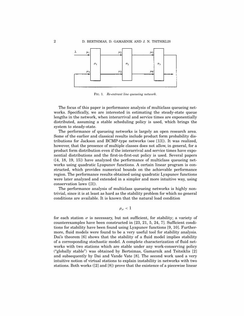
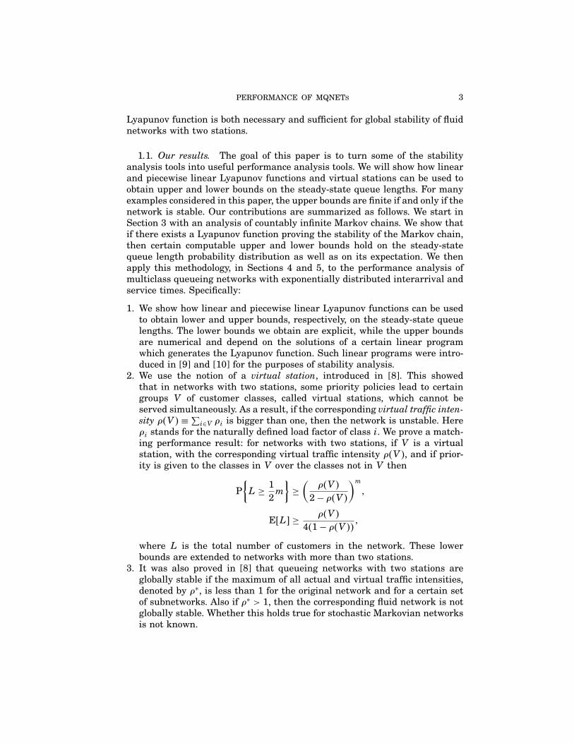
1. Introduction. Queueing networks are used to model manufacturing,communication and computer systems, and much recent research has focusedon networks with multiple customer classes. In multiclass queueing networks,the customers served at the same station have in general different servicerequirements and follow different paths through the network. Such networksare used to model, for example, wafer fabrication facilities, in which there is asingle stream of jobs arriving into a production floor. Jobs follow a determinis-tic route and revisit the same station multiple times (see Figure 1). Multiclassqueueing networks of this type are called reentrant line queueing networks(see [17, 9]).
Received March 2000; revised February 2001.1Research supported in part by NSF Grants DMI-96-10486, ACI-98-73339, ARO Grant DAAL-
03-92-G-0115 and by the Singapore-MIT alliance.AMS 2000 subject classifications.Key words and phrases.
1
2 D. BERTSIMAS, D. GAMARNIK AND J. N. TSITSIKLIS
Fig. 1. Re-entrant line queueing network.
The focus of this paper is performance analysis of multiclass queueing net-works. Specifically, we are interested in estimating the steady-state queuelengths in the network, when interarrival and service times are exponentiallydistributed, assuming a stable scheduling policy is used, which brings thesystem to steady-state.The performance of queueing networks is largely an open research area.
Some of the earlier and classical results include product form probability dis-tributions for Jackson and BCMP-type networks (see [13]). It was realized,however, that the presence of multiple classes does not allow, in general, for aproduct form distribution even if the interarrival and service times have expo-nential distributions and the first-in-first-out policy is used. Several papers([4, 18, 19, 15]) have analyzed the performance of multiclass queueing net-works using quadratic Lyapunov functions. A certain linear program is con-structed, which provides numerical bounds on the achievable performanceregion. The performance results obtained using quadratic Lyapunov functionswere later analyzed and extended in a simpler and more intuitive way, usingconservation laws ([3]).The performance analysis of multiclass queueing networks is highly non-
trivial, since it is at least as hard as the stability problem for which no generalconditions are available. It is known that the natural load condition
ρσ < 1
for each station σ is necessary, but not sufficient, for stability; a variety ofcounterexamples have been constructed in [23, 21, 5, 24, 7]. Sufficient condi-tions for stability have been found using Lyapunov functions [9, 10]. Further-more, fluid models were found to be a very useful tool for stability analysis.Dai’s theorem [6] shows that the stability of a fluid model implies stabilityof a corresponding stochastic model. A complete characterization of fluid net-works with two stations which are stable under any work-conserving policy(“globally stable”) was obtained by Bertsimas, Gamarnik and Tsitsiklis [2]and subsequently by Dai and Vande Vate [8]. The second work used a veryintuitive notion of virtual stations to explain instability in networks with twostations. Both works ([2] and [8]) prove that the existence of a piecewise linear
PERFORMANCE OF MQNETs 3
Lyapunov function is both necessary and sufficient for global stability of fluidnetworks with two stations.
1.1. Our results. The goal of this paper is to turn some of the stabilityanalysis tools into useful performance analysis tools. We will show how linearand piecewise linear Lyapunov functions and virtual stations can be used toobtain upper and lower bounds on the steady-state queue lengths. For manyexamples considered in this paper, the upper bounds are finite if and only if thenetwork is stable. Our contributions are summarized as follows. We start inSection 3 with an analysis of countably infinite Markov chains. We show thatif there exists a Lyapunov function proving the stability of the Markov chain,then certain computable upper and lower bounds hold on the steady-statequeue length probability distribution as well as on its expectation. We thenapply this methodology, in Sections 4 and 5, to the performance analysis ofmulticlass queueing networks with exponentially distributed interarrival andservice times. Specifically:
1. We show how linear and piecewise linear Lyapunov functions can be usedto obtain lower and upper bounds, respectively, on the steady-state queuelengths. The lower bounds we obtain are explicit, while the upper boundsare numerical and depend on the solutions of a certain linear programwhich generates the Lyapunov function. Such linear programs were intro-duced in [9] and [10] for the purposes of stability analysis.
2. We use the notion of a virtual station, introduced in [8]. This showedthat in networks with two stations, some priority policies lead to certaingroups V of customer classes, called virtual stations, which cannot beserved simultaneously. As a result, if the corresponding virtual traffic inten-sity ρ�V� ≡∑
i∈V ρi is bigger than one, then the network is unstable. Hereρi stands for the naturally defined load factor of class i. We prove a match-ing performance result: for networks with two stations, if V is a virtualstation, with the corresponding virtual traffic intensity ρ�V�, and if prior-ity is given to the classes in V over the classes not in V then
P{L ≥ 1
2m
}≥(
ρ�V�2− ρ�V�
)m
E�L� ≥ ρ�V�4�1− ρ�V��
where L is the total number of customers in the network. These lowerbounds are extended to networks with more than two stations.
3. It was also proved in [8] that queueing networks with two stations areglobally stable if the maximum of all actual and virtual traffic intensities,denoted by ρ∗, is less than 1 for the original network and for a certain setof subnetworks. Also if ρ∗ > 1, then the corresponding fluid network is notglobally stable. Whether this holds true for stochastic Markovian networksis not known.
4 D. BERTSIMAS, D. GAMARNIK AND J. N. TSITSIKLIS
We show that ρ∗ is a fundamental performance parameter. For reentrantline networks with two stations, we show that if ρ∗ < 1, then the followingupper bound holds under any work-conserving policy:
E�L� ≤ C
�1− ρ∗�2
where C is some constant, expressed explicitly in terms of the parametersof the network. An important implication of this result is that the perfor-mance region (the set of vectors of expected queue lengths obtained underdifferent work-conserving scheduling policies) is bounded if and only if thecorresponding fluid network is globally stable.
Our results show a deeper connection between stability and performanceof multiclass queueing networks. Also the results in this paper are the firstones that use linear and piecewise linear Lyapunov functions for performanceanalysis. Previous methods for performance analysis have used quadraticLyapunov functions, which have certain limitations. In particular, an exam-ple of a globally stable queueing network with two stations was constructedin [10] for which the quadratic Lyapunov function method leads to an infinite(inconclusive) upper bound, yet a piecewise linear Lyapunov function gives afinite upper bound. The methods developed here, on the other hand, match thesharpest known stability condition ρ∗ < 1. The second limitation of quadraticLyapunov functions is that the bounds constructed are in most cases onlynumerical and hold only for the expectations of queue lengths. In contrast,we provide bounds on the distribution of steady-state queue lengths, provingexponential decay of the tail probabilities.
2. Queueing model and assumptions.
2.1. Multiclass Markovian queueing network. We consider a network con-sisting of J single server stations, which are denoted by σj j = 12 � � � J.The network includes I types of customers, where customers of type i = 1,2 � � � I arrive to the network from an exogenous source. The arrival pro-cess corresponding to type i is assumed to be an independent Poisson processwith rate λi. Let � = �λ1 � � � λI� denote the vector of arrival rates and letλmin = mini�λi . Without loss of generality, we assume that λmin > 0. Simi-larly, we define λmax = maxi�λi . Customers of type i go through Ji stages,each of which corresponds to a service completion on a particular station. Wedenote these stations by σi1 σi2 � � � σiJi . The processing time of a type icustomer at station σik k = 12 � � � Ji, is assumed to be exponentially dis-tributed with rate µik and is independent from the processing times of allother stages of this type, from the processing times of the other types andfrom the interarrival times. We let � = �µik�1≤i≤I1≤k≤Ji denote the vector ofservice rates. Customers of type i receiving service at station σik are calledclass �i k� customers. Let N = ∑I
i=1Ji be the total number of classes. For
PERFORMANCE OF MQNETs 5
convenience, we will also identify every station σj with the set of classes asso-ciated with this station. Let Cik = j if class �i k� customers are served atstation σj. For k ≥ Ji we let Cik = 0. Let C denote the corresponding I×Jmaxmatrix, where Jmax = maxi Ji. The matrix C defines the topology of the net-work. We assume that the buffers at each station have infinite capacity andno customers renege from the queue before receiving service.A queueing network of the form just described is called a Markovian mul-
ticlass queueing network with deterministic routing or a multitype queueingnetwork. Throughout the paper we consider only networks of this type. Theparameters ��C constitute the primary parameters of the network and wedenote the network by ���C�.For each class �i k�, we let ρik = λi/µi k be the nominal load of this
class. For each station σj j = 12 � � � J, we define the nominal load (trafficintensity) as
ρσj ≡∑
�i k�∈σjρik�(1)
The evolution of a queueing network is fully specified only when a schedul-ing discipline is given. The scheduling discipline (policy) describes which cust-omers (if any) are served at any moment at each station. Within each class, thecustomers are served in first-in-first-out (FIFO) fashion. Therefore, the servicediscipline only specifies which customer type is served at any given moment.We will assume throughout the paper that the scheduling policies imple-mented are Markovian, namely, scheduling decisions are purely a function ofthe system state, which in our case is the vector of all queue lengths. We alsoallow preemption. For example, preemptive priority policies are Markovian.Many important policies are not Markovian, for example FIFO or head-of-the-line-processor-sharing. We leave these policies out from the discussion inthis paper, although we believe that the results hold for them as well. Wewill be considering mostly work-conserving policies: each processing station isrequired to work on some customer, if there are any present at this station.Any preemptive policy w satisfying the Markovian assumption can be des-
cribed by a function w� ZN+ → �01 N where for any q ∈ ZN
+ , the �i k�component of the vectorw�q� is 1 if station σj which contains class �i k�workson a customer of class �i k�, and is zero, otherwise. Of course, wik�q� = 1only if qik > 0, and for each station σj,∑
�i k�∈σjwik�q� ≤ 1�(2)
Given a multiclass queueing network ���C� and some scheduling policy,we let Q�t� = �Qik�t��1≤i≤I1≤k≤Ji denote the vector of queue lengths at timet. Our focus is on estimating the distribution of the random vector Q�t� insteady-state. A necessary condition for the existence of a steady-state is the
6 D. BERTSIMAS, D. GAMARNIK AND J. N. TSITSIKLIS
load condition
ρσj < 1(3)
for each j = 12 � � � J.
2.2. Embedded Markov chains and uniformization. Instead of analyzingthe continuous time processQ�t�, we will build a discrete time analogue, whichhas the same steady-state behavior using the standard method of uniformiza-tion (see [20]). We rescale the parameters, so that
∑i λi +
∑i k µi k = 1 and
consider a superposition of I +∑Ii=1Ji Poisson processes with rates λi µi k,
respectively. The arrivals of the first I Poisson processes correspond to externalarrivals into the network. The arrivals of the process with rate µik correspondto service completions of class �i k� customers, if a server actually worked ona class �i k� customer, or they correspond to “imaginary” service completionsof an “imaginary” customer, if the server was idle or worked on customersfrom other classes. Let τs s = 12 � � � be the sequence of event times for thissuperposition of Poisson processes. Then, as a result of this construction andthe Markovian policy assumption, Q�τs� is a discrete time Markov chain withthe same steady-state distribution as Q�t� (assuming it exists).We can specify the transitions of the Markov chainQ�τs� as follows. For each
class �i k� let ei k be anN-dimensional unit vector with the �i k� componentequal to 1 and all other components equal to zero. We adopt the conventionei0 = eiJi+1 = 0 for each i. The following proposition holds.
Proposition 1. Given a multiclass queueing network ���C� rescaled sothat
∑i λi+
∑i k µi k = 1 and given a Markovian policy w, the transition prob-
abilities of the corresponding embedded Markov chain Q�τs� s = 012 � � � aregiven by
Q�τs+1�=
Q�τs�+ei1 with probability λi,Q�τs�−eik+eik+1 with probability µikwik�Q�τs��,Q�τs� with probability
∑ik
µik�1−wikQ�τs��.(4)
Proof. Note that the change Q�τs+1� − Q�τs� of the embedded Markovchain corresponds to either an arrival of a type i customer, or to an “actual”service completion of a class �i k� customer and transition to the next stagek + 1. The first event has a probability λi and corresponds to a change ei1.The second event has probability µikwik�Q�τs�� and corresponds to a changeei k+1 − ei k. ✷
Definition 1. A scheduling policy w is defined to be stable if the corre-sponding embedded Markov chain Q�τs� s = 12 � � � , admits a stationaryprobability distribution π = π�w� satisfying∑
i k
E�Qik�τs�� <∞�(5)
PERFORMANCE OF MQNETs 7
A queueing network is defined to be globally stable if every work-conservingMarkovian policy is stable.
If a stationary distribution π of Q�τs� exists, then by uniformization andby aperiodicity of our continuous time Markov chain,
limt→∞
P�Q�t� = q = P{Q�τs� = q}�(6)
Thus, for performance analysis purposes, we may concentrate on the embeddedchain Q�τs�.Throughout the paper we use standard notations O�·���·���·� in the
following sense. If functions f�s� g�s� → ∞ when s → s0 for some s0 ∈�−∞+∞�, then g = O�f��g = ��f�� means that for some fixed constantc > 0, g�s� ≤ cf�s��g�s� ≥ cf�s�� for sufficiently large s. If g = O�f� we willalso write f = O�g�. If both g = O�f� f = O�g�, then we will write g = ��f�.
3. Infinite Markov chains and Lyapunov functions. In this section,we develop a general technique for steady-state analysis of infinite Markovchains with countably many states using Lyapunov functions.Let X�t� t = 012 � � � , be a discrete time, discrete state Markov chain
which takes values in some countable set � . The transitions occur at integertimes t = 012 � � � . For any two vector xx′ ∈ � , let p�xx′� denote thetransition probabilities
p�xx′� ≡ P{X�t+ 1� = x′�X�t� = x}�
If a stationary probability distribution π on the state space� exists, it satisfies∑x∈�
π�x� = 1
and for all x ∈ � ,
π�x� = ∑x′∈�
π�x′�p�x′x��(7)
The existence of a stationary distribution is usually established by construct-ing a certain Lyapunov function. For a survey of Lyapunov methods for sta-bility analysis of Markov chains, see [22]. We now introduce the definitions ofLyapunov and lower Lyapunov functions. The goal is to use Lyapunov func-tions for the performance analysis of Markov chains, assuming a priori thatthe Markov chain is stable. The notion of a lower Lyapunov function is intro-duced exclusively as a means of getting the lower bounds on the stationarydistribution of a Markov chain. In subsequent sections, we apply the resultshere to the embedded Markov chain of a multiclass queueing network.
Definition 2. A nonnegative function
$� � → �+
8 D. BERTSIMAS, D. GAMARNIK AND J. N. TSITSIKLIS
is said to be a Lyapunov function if there exist some γ > 0 and B ≥ 0, suchthat for any t = 12 � � � and any x ∈ � , with $�x� > B,
E[$�X�t+ 1���X�t� = x
] ≤ $�x� − γ�(8)
Also a nonnegative function
$� � → �+(9)
is said to be a lower Lyapunov function if there exists some γ > 0, such thatfor any t = 12 � � � and any x ∈ � , with $�x� > 0,
E[$�X�t+ 1���X�t� = x
] ≥ $�x� − γ�
Remarks.
(i) We refer to the terms γ and B as drift and exception parameters,respectively.(ii) We could also introduce an exception parameter B for the lower
Lyapunov function, but it is not required for the examples in this paper.
We assume that the Markov chain X�t� is positive recurrent, and we denoteby π the corresponding stationary distribution. Namely, π�x� is the steady-state probability Pπ�X�t� = x that the chain is in a certain state x ∈ � .Also, we denote by Eπ�·� the expectation with respect to the probability distri-bution π. For a given function $� � → �+, let
νmax ≡ supxx′∈� � p�xx′�>0
�$�x′� −$�x��(10)
and
νmin ≡ infxx′∈� � p�xx′�>0$�x�<$�x′�
�$�x′� −$�x���(11)
Namely, νmax is the largest possible change of the function $ during an arbi-trary transition, and νmin is the smallest possible increase of the function $.Also let
pmax = supx∈�
∑x′∈� $�x�<$�x′�
p�xx′�(12)
and
pmin = infx∈�
∑x′∈� $�x�<$�x′�
p�xx′��(13)
Namely, pmax and pmin are tight upper and lower bounds on the probabil-ity that the value of $ is increasing during an arbitrary transition. In thispaper, we will be interested in Lyapunov functions with finite νmax, and lowerLyapunov functions with positive νmin and pmin. We need the following lemma,the proof of which can be found in Appendix A.
PERFORMANCE OF MQNETs 9
Lemma 1. Consider a Markov chain X�t� with stationary probability distri-bution π, and suppose that $ is a Lyapunov function with drift γ and exceptionparameter B, such that Eπ�$�X�t�� is finite. Then, for any (possibly negative)c ≥ B− νmax,
Pπ{c+ νmax < $�X�t��} ≤ pmaxνmax
pmaxνmax + γPπ{c− νmax < $�X�t��}(14)
where νmax and pmax are defined in (10) and (12), respectively. Also, if $ is alower Lyapunov function with drift γ, such that Eπ�$�X�t��� is finite, then, forany c ≥ 0,
Pπ{c ≤ $�X�t��} ≥ pminνmin
pminνmin + 2γPπ
{c− 1
2νmin ≤ $�X�t��
}(15)
where νmin and pmin are defined in (11) and (13), respectively.
This lemma shows how one can obtain a simple recurrence relation on thetail probabilities Pπ�c < $�X�t�� . We use this recurrence in the proof of thefollowing result.
Theorem 1. Consider a Markov chain X�t� with a stationary probabilitydistribution π such that Eπ�$�X�t��� <∞.
(i) If there exists a Lyapunov function $ with drift γ > 0, and exceptionparameter B ≥ 0, then for any m = 012 � � � ,
Pπ{$�X�t�� > B+ 2νmaxm
} ≤ (pmaxνmax
pmaxνmax + γ
)m+1�(16)
As a result,
Eπ�$�X�t��� ≤ B+ 2pmax�νmax�2γ
�(17)
(ii) If there exists a lower Lyapunov function $ with drift γ > 0, then forany m = 012 � � � ,
Pπ{$�X�t�� ≥ �1/2�νminm
} ≥ ( �1/2�pminνmin�1/2�pminνmin + γ
)m�(18)
As a result,
Eπ�$�X�t��� ≥pmin�νmin�2
4γ�(19)
Remark. The bounds (16), (17) and (18), (19) are meaningful only if νmax <∞ (the Lyapunov function has uniformly bounded jumps) and νmin pmin > 0,respectively.
10 D. BERTSIMAS, D. GAMARNIK AND J. N. TSITSIKLIS
Proof. In order to prove (16), we let c = B− νmax. By applying Lemma 1,we obtain
Pπ�B < $�X�t�� ≤ pmaxνmaxpmaxνmax + γ
Pπ{B− 2νmax < $�X�t��}
≤ pmaxνmaxpmaxνmax + γ
�
We continue similarly, using c = B + νmax c = B + 3νmax c = B + 5νmax � � � .By applying again Lemma 1, we obtain the needed upper bound on the taildistribution.In order to prove (17), note that
Eπ�$�X�t��� ≤ B·Pπ�$�X�t��≤B +∞∑m=0
�B+2νmax�m+1��
×Pπ{B+2νmaxm<$�X�t��≤B+2νmax�m+1�}
= B·Pπ�$�X�t��≤B
+B∞∑m=0
Pπ{B+2νmaxm<$�X�t��≤B+2νmax�m+1�}
+2νmax∞∑m=0
�m+1�Pπ{B+2νmaxm<$�X�t��≤B+2νmax�m+1�}�
However,
∞∑m=0
�m+ 1�Pπ{B+ 2νmaxm < $�X�t�� ≤ B+ 2νmax�m+ 1�}
=∞∑m=0
Pπ{B+ 2νmaxm < $�X�t��}�
Applying the bounds from (16), we obtain
Eπ�$�X�t��� ≤ B+ 2νmax∞∑m=0
(pmaxνmax
pmaxνmax + γ
)m+1
= B+ 2pmax�νmax�2γ
�
To prove (18), let c = νmin/2 c = νmin c = 3νmin/2 � � � . Then, by applyingLemma 1, we obtain
Pπ{$�X�t�� ≥ �1/2�νminm
} ≥ ( �1/2�pminνmin�1/2�pminνmin + γ
)mPπ�$�X�t�� ≥ 0
=( �1/2�pminνmin�1/2�pminνmin + γ
)m�
PERFORMANCE OF MQNETs 11
In order to prove (19), we have
Eπ�$�X�t��� ≥ 12
∞∑m=0
νminmPπ{�1/2�νminm ≤ $�X�t�� < �1/2�νmin�m+ 1�}
= 12νmin
∞∑m=1
Pπ{�1/2�νminm ≤ $�X�t��}�
From (18) we obtain
Eπ�$�X�t��� ≥12νmin
∞∑m=1
( �1/2�pmin νmin�1/2�pmin νmin + γ
)m= pmin�νmin�2
4γ�
This completes the proof of the theorem. ✷
As mentioned above, the steady-state behavior of Markovian queueing net-works is equivalent to the steady-state behavior of the embedded Markovchain. Applying Theorem 1, we can analyze the performance of Markovianqueueing networks by constructing suitable Lyapunov functions. This is thesubject of the following sections.
4. Lower bounds on queue lengths using linear lower Lyapunovfunctions. In this section, we use linear lower Lyapunov functions to findclosed form lower bounds on the distribution and expectation of steady-statequeue lengths, which hold when an arbitrary stable Markovian schedulingpolicy is implemented.Given a stable scheduling policy w, let π = π�w� denote the corresponding
stationary distribution (of the queueing network and its embedded Markovchain). We will show that
Eπ
[∑i k
Qik�t�]= �
(J∑j=1
11− ρσj
)= �
(1
1− ρ
)
where ρσj is the traffic intensity at station σj and ρ = max1≤j≤J�ρσj . We willalso derive lower bounds on the distribution and expected queue lengths whichhold specifically when priority policies are implemented, by using the notionof a virtual station. Finally, we will apply these results to some examples.
4.1. Closed form lower bounds for arbitrary work-conserving policies. Recallthat under any Markovian scheduling policy, the transitions of the uniformizedembedded Markov chain are given by Proposition 1. For each station σj, wenow construct a lower Lyapunov function. For any class �i k�, let
ρσj+i k = ∑
k′ � �i k′�∈σj k′≥kρi k′ �(20)
12 D. BERTSIMAS, D. GAMARNIK AND J. N. TSITSIKLIS
In words, ρσj+i k is the sum of traffic intensities of classes of type i starting from
stage k onward which are processed on station σj. Let
$j�Q� =∑i k
ρσj+i k
λiQik�
Proposition 2. Let w be an arbitrary Markovian policy. Then, $j is alower Lyapunov function with drift γj = 1 − ρσj and pmin = ∑
i λi νmin ≥ρσj/λmax.
Proof. Using Proposition 1, we have
E�$j�Q�τs+1���Q�τs�� = $j�Q�τs�� +I∑i=1
λiρσj+i1
λi
+ ∑i k
µi kwik�Q�τs��(ρσj+i k+1 − ρ
σj+i k
)/λi�
(21)
Note from (20) that
I∑i=1
λiρσj+i1
λi=
I∑i=1
∑k′ � �i k′�∈σjk′≥1
ρik′ = ρσj�
Observe that for any class �i k� ∈ σj,∑�i k�∈σj
µi kwik�Q�τs��(ρσj+i k+1 − ρ
σj+i k
)/λi =
∑�i k�∈σj
µi kwik�Q�τs��(−ρikλi
)= − ∑
�i k�∈σjwik�Q�τs�� ≥ −1
where the last equality follows from the feasibility constraint (2) for the policyw. Also note that ρ
σj+i k+1 − ρ
σj+i k = 0 when �i k� �∈ σj. Combining with (21) we
obtain
E[$j�Q�τs+1���Q�τs�
]−$j�Q�τs�� ≥ ρσj − 1�This proves that $j is a lower Lyapunov function. We now bound the param-eters νmin and pmin. From Proposition 1, if a transition of the Markov chainQ�τs� corresponds to a service completion in the class �i k�, then the corre-sponding change in the value of the Lyapunov function $j is
−ρσj+i k /λi + ρσj+i k+1/λi
which by definition is nonpositive. Therefore, the value of the Lyapunov func-tion can increase only at the arrival times and, as a result, pmin =
∑Ii=1 λi. At
an arrival of a type i customer, the value of the Lyapunov function increasesby ρσj/λi. Therefore νmin ≥ ρσj/λmax. ✷
PERFORMANCE OF MQNETs 13
We now are ready to state the main result of this section.
Theorem 2. Consider a multiclass queueing network ���C� operatingunder an arbitrary stable Markovian policy. The following lower bounds holdon the steady-state number of customers in the network: for each j = 12 � � � J,and m = 012 � � � ,
P
{∑i k
ρσj+i k
λiQik�t� ≥
ρσj2λmax
m
}≥( ρσj2− ρσj
)m ∗
and
E
[∑i k
ρσj+i k
λiQik�t�
]≥
ρ2σj4λmax�1− ρσj�
�
The result follows by applying Proposition 2 and Theorem 1.
Remarks.
(i) The bounds hold whether we have rescaled the parameters to∑i λi +∑
i k µi k=1 or not, since ρσj , and the ratio λi/λmax are insensitive to rescaling.(ii) The bounds hold whether the policy used is work-conserving or not.
The bounds of Theorem 2 are simplified when the multiclass queueing net-work has a reentrant line structure, namely, I = 1. In this case, all customersfollow the same route in the network. We denote by Qk�t� the queue length atthe kth stage in the network. The parameters ρik ρ
σj+i k are denoted simply by
ρk and ρσj+k . The lower bounds on the queue lengths are simplified as follows.
Corollary 1. Given a reentrant line-type queueing network ���C�, ope-rating under any stable Markovian policy, the following lower bounds holdon the number of customers in the network in steady-state. For each j = 1,2 � � � J, and m = 012 � � � ,
P{∑
k
ρσj+k Qk�t� ≥
ρσj2m
}≥( ρσj2− ρσj
)m
and
E[∑k
ρσj+k Qk�t�
]≥
ρ2σj4�1− ρσj�
�
4.2. Closed form lower bounds under a priority policy. In this section, wederive lower bounds on the tail probabilities and the expected number of cus-tomers in a multiclass queueing network operating under a priority policy wθ
that is described by a permutation θ of the set of classes ��i k� 1≤i≤I1≤k≤Ji .For two classes �i k� �i′ k′� associated with the same station σj, we saythat class �i′ k′� has a higher priority than class �i k� if θ�i′ k′� < θ�i k�.
14 D. BERTSIMAS, D. GAMARNIK AND J. N. TSITSIKLIS
A corresponding priority policy wθ can be described as follows: for each stateq ∈ ZN
+ wθ�q� is an N-dimensional binary vector whose components satisfywθik�q� = 1
if and only if qik > 0 and qi′ k′ = 0, whenever �i′ k′� ∈ σj, where j is suchthat �i k� ∈ σj, and θ�i′ k′� < θ�i k�. In other words, the policy wθ at eachtransition epoch τs, selects within each station σj the highest priority classwith a positive number of customers and works on a customer from this class.We thus assume that wθ is a preemptive resume priority policy. Clearly, pre-emptive priority policies are Markovian.The lower bounds to be derived in this section are based on the concept of a
virtual station and virtual traffic intensity introduced in [8], where the virtualstation concept is used for the stability analysis. We will show how virtualstations characterize the performance of multiclass queueing networks. Thedefinitions below follow [8] very closely.
Definition 3. A collection of classes e = ��i k1� �i k1 + 1� � � � �i k2� ,corresponding to a type-i customer is defined to be an excursion if all theseclasses are from some station σj, but classes �i k1− 1� and �i k2+ 1� are notfrom station σj. This includes the possibility k1 = 1 or k2 = Ji. The classes�i k1� � � � �i k2 − 1� are called the first classes of the excursion e and class�i k2� is called the last class of the excursion e.
We denote the sequence of all excursions corresponding to type i by ei1,ei2 � � � e
iR.
Definition 4. Given a multiclass queueing network ���C�, supposethat a collection of stations + ⊂ �σ1 σ2 � � � σJ with size �+� = K, andnonempty collections of classes Vj ⊂ σj j ∈ + are selected. The set of classesV = ∪j∈SVj is defined to be a K-virtual (or just a virtual) station if thefollowing conditions hold:
(i) No classes of the first excursion are in V� ei1 ∩ V = ∅, for each i =12 � � � I.(ii) If the last class of some excursion eil is in V, then all the classes of this
excursion are in V, and if a first class of the excursion eil is in V, then everyfirst class of eil is in V. Thus, a virtual station must have either none of theclasses, all of the classes, or all but the last class of each excursion.(iii) If a class �i k� is the first class of an excursion eil with l �= 1 [that is
σ�i k− 1� �= σ�i k�], then class �i k� ∈ V if and only if �i k− 1� �∈ V.
For example, Classes 2, 3 and 5 in the reentrant line network in Figure 2,constitute a 2-virtual station. The following result was proved in [1] and [14].
Proposition 3. Suppose that a set of classes V = ∪j∈+Vj forms a K-virtual station for some + ⊂ �12 � � � J and that wθ is a stable priority
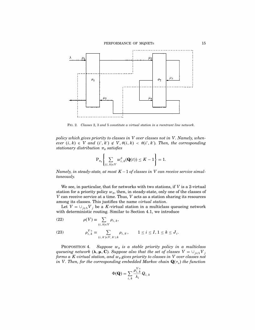
PERFORMANCE OF MQNETs 15
Fig. 2. Classes 2, 3 and 5 constitute a virtual station in a reentrant line network.
policy which gives priority to classes in V over classes not in V. Namely, when-ever �i k� ∈ V and �i′ k′� �∈ Vθ�i k� < θ�i′ k′�. Then, the correspondingstationary distribution πθ satisfies
Pπθ
{ ∑�i k�∈V
wθi k�Q�t�� ≤K− 1
}= 1�
Namely, in steady-state, at most K−1 of classes in V can receive service simul-taneously.
We see, in particular, that for networks with two stations, if V is a 2-virtualstation for a priority policy wθ, then, in steady-state, only one of the classes ofV can receive service at a time. Thus, V acts as a station sharing its resourcesamong its classes. This justifies the name virtual station.Let V = ∪j∈+Vj be a K-virtual station in a multiclass queueing network
with deterministic routing. Similar to Section 4.1, we introduce
ρ�V� ≡ ∑�i k�∈V
ρik(22)
ρV+i k ≡ ∑
�i k′�∈Vk′≥kρi k′ 1 ≤ i ≤ I1 ≤ k ≤ Ji�(23)
Proposition 4. Suppose wθ is a stable priority policy in a multiclassqueueing network ���C�. Suppose also that the set of classes V = ∪j∈+Vj
forms a K-virtual station, and wθ gives priority to classes in V over classes notin V. Then, for the corresponding embedded Markov chain Q�τs� the function
$�Q� =∑i k
ρV+i k
λiQik
16 D. BERTSIMAS, D. GAMARNIK AND J. N. TSITSIKLIS
is a lower Lyapunov function with drift K− 1−ρ�V� pmin =∑i λi and νmin ≥
ρ�V�/λmax.
Proof. From Proposition 1 in Section 2, we have
E�$�Q�τs+1���Q�τs�� −$�Q�τs��
=I∑i=1
λiρV+i1
λi+∑
i k
µi kwθi k�Q�τs��
1λi
(ρV+i k+1 − ρV+
i k
)
where we assume that ρV+iJi+1 = 0. Note that
ρV+i k+1 − ρV+
i k ={−ρik if �i k� ∈ V,0 if �i k� �∈ V.
Therefore,
E�$�Q�τs+1���Q�τs�� −$�Q�τs�� =∑i
ρV+i1 − ∑
�i k�∈Vwθi k�Q�τs���
From Proposition 3 and from∑i ρ
V+i1 = ρ�V� we obtain that the drift is γ =
K − 1 − ρ�V�. We obtain the expressions for pmin and νmin as in the proof ofProposition 2. ✷
A corollary of this result is the transience (instability) of a priority policywθ if for some virtual station V, we have ρ�V� > K−1. This instability resultwas proven in [1] and [14] under more general assumptions, interarrival andservice times have a general (as opposed to exponential) distribution. We nowderive a matching performance result, when ρ�V� < K − 1. The followingtheorem is the main result of this section.
Theorem 3. Suppose we are given a multiclass queueing network ���C�,and a set of classes V that forms a K-virtual station. If a stable priority policywθ gives priority to classes in V over the classes outside V, then the followinglower bounds hold on the steady-state distribution and expectation of the num-ber of customers in the network. For each j = 12 � � � J, and m = 012 � � � ,
P
{∑i k
ρV+i k
λiQik�t� ≥
ρ�V�2λmax
m
}≥(
ρ�V�2�K− 1� − ρ�V�
)mand
E
[∑i k
ρV+i k
λiQik�t�
]≥ ρ2�V�4λmax�K− 1− ρ�V�� �
The proof is similar to the one of Theorem 2.The lower bounds of Theorem 3 are also simplified when the network is
reentrant line-type.
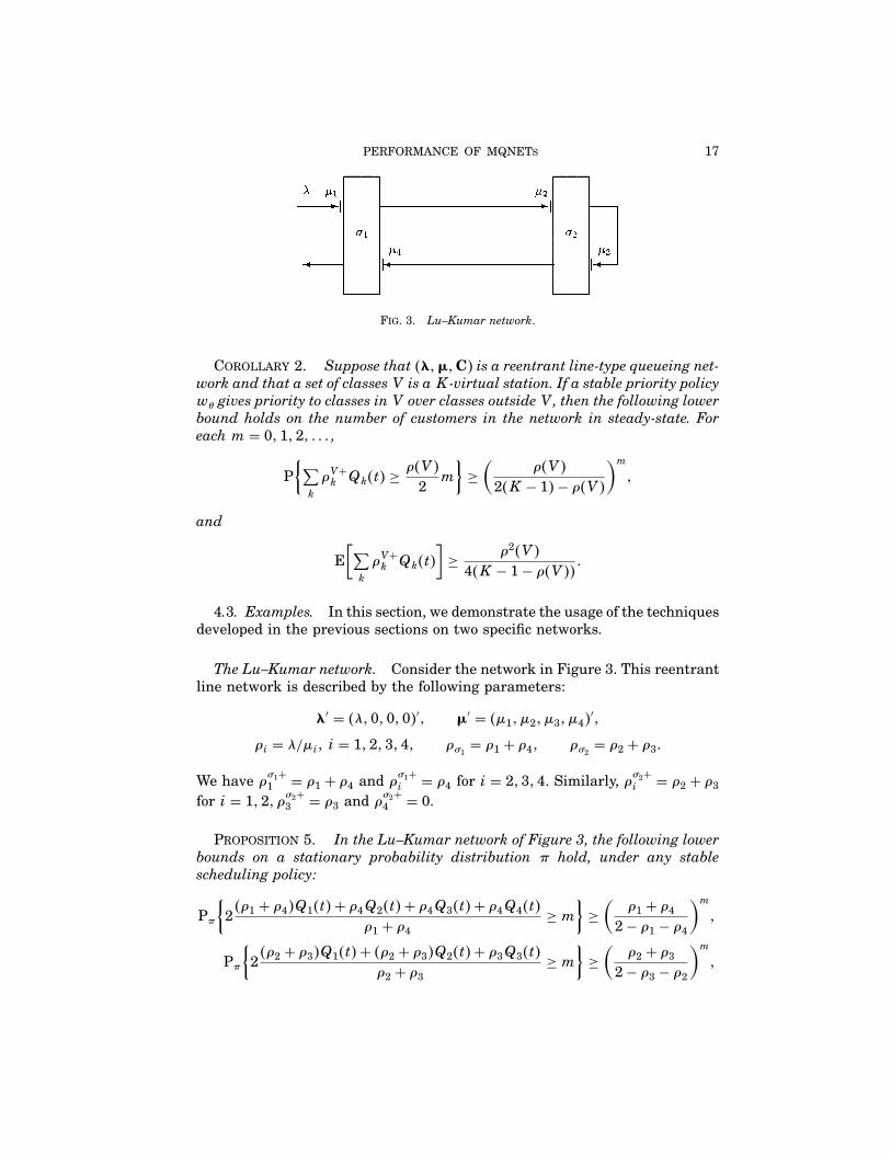
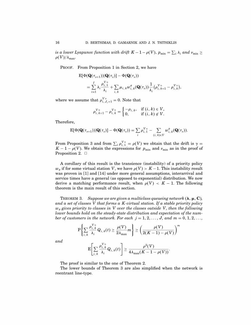
PERFORMANCE OF MQNETs 17
Fig. 3. Lu–Kumar network.
Corollary 2. Suppose that ���C� is a reentrant line-type queueing net-work and that a set of classesV is aK-virtual station. If a stable priority policywθ gives priority to classes in V over classes outside V, then the following lowerbound holds on the number of customers in the network in steady-state. Foreach m = 012 � � � ,
P{∑
k
ρV+k Qk�t� ≥
ρ�V�2
m
}≥(
ρ�V�2�K− 1� − ρ�V�
)m
and
E[∑k
ρV+k Qk�t�
]≥ ρ2�V�4�K− 1− ρ�V�� �
4.3. Examples. In this section, we demonstrate the usage of the techniquesdeveloped in the previous sections on two specific networks.
The Lu–Kumar network. Consider the network in Figure 3. This reentrantline network is described by the following parameters:
�′ = �λ000�′ �′ = �µ1 µ2 µ3 µ4�′ρi = λ/µi i = 1234 ρσ1 = ρ1 + ρ4 ρσ2 = ρ2 + ρ3�
We have ρσ1+1 = ρ1 + ρ4 and ρσ1+i = ρ4 for i = 234. Similarly, ρσ2+i = ρ2 + ρ3
for i = 12 ρσ2+3 = ρ3 and ρσ2+4 = 0.
Proposition 5. In the Lu–Kumar network of Figure 3, the following lowerbounds on a stationary probability distribution π hold, under any stablescheduling policy:
Pπ
{2�ρ1 + ρ4�Q1�t� + ρ4Q2�t� + ρ4Q3�t� + ρ4Q4�t�
ρ1 + ρ4≥m
}≥(
ρ1 + ρ42− ρ1 − ρ4
)m
Pπ
{2�ρ2 + ρ3�Q1�t� + �ρ2 + ρ3�Q2�t� + ρ3Q3�t�
ρ2 + ρ3≥m
}≥(
ρ2 + ρ32− ρ3 − ρ2
)m
18 D. BERTSIMAS, D. GAMARNIK AND J. N. TSITSIKLIS
for all m = 012 � � � . Also
Eπ[�ρ1 + ρ4�Q1�t� + ρ4Q2�t� + ρ4Q3�t� + ρ4Q4�t�
] ≥ 14
�ρ1 + ρ4�2�1− ρ1 − ρ4�
Eπ[�ρ2 + ρ3�Q1�t� + �ρ2 + ρ3�Q2�t� + ρ3Q3�t�
] ≥ 14
�ρ2 + ρ3�2�1− ρ2 − ρ3�
�
If, in addition, the network operates under priority policy wθ with priority ruleθ�4� < θ�1� θ�2� < θ�3�, then
Pπθ
{2�ρ2 + ρ4�Q1�t� + �ρ2 + ρ4�Q2�t� + ρ4Q3�t� + ρ4Q4�t�
ρ2 + ρ4≥m
}≥(
ρ2 + ρ42− ρ2 − ρ4
)m
for all m = 012 � � � , and
Eπθ[�ρ2 + ρ4�Q1�t� + �ρ2 + ρ4�Q2�t� + ρ4Q3�t� + ρ4Q4�t�
](24)
≥ 14
�ρ2 + ρ4�2�1− ρ2 − ρ4�
�
The first part of the proposition is obtained by applying Corollary 1 tostations σ1 and σ2, the second part is obtained by applying Corollary 2 tothe virtual station V = �24 .
A 3-station, 6-class reentrant line. Consider the reentrant line queueingnetwork with six classes and three stations described in Figure 1. This networkwas considered in [7], where the authors introduce the priority rule θ withθ�4� < θ�1� θ�2� < θ�5� θ�6� < θ�3� and show that the set V = �246 forms a 3-virtual station. Applying Corollary 2 we obtain the following result.
Proposition 6. Consider the network in Figure 1, under the priority ruleθ�4� < θ�1� θ�2� < θ�5� θ�6� < θ�3�. Suppose in addition that the policy isstable. Then, for the corresponding stationary probability distribution πθ,
Pπθ
{2�ρ2 + ρ4 + ρ6�Q1�t� + �ρ2 + ρ4 + ρ6�Q2�t� + �ρ4 + ρ6�Q3�t�
ρ2 + ρ4 + ρ6
+ �ρ4 + ρ6�Q4�t� + ρ6Q5�t� + ρ6Q6�t�ρ2 + ρ4 + ρ6
≥m
}≥(
ρ2 + ρ4 + ρ64− ρ2 − ρ4 − ρ6
)m
for each m = 012 � � � .Also,
Eπθ[�ρ2 + ρ4 + ρ6�Q1�t� + �ρ2 + ρ4 + ρ6�Q2�t� + �ρ4 + ρ6�Q3�t�
+ �ρ4 + ρ6�Q4�t� + ρ6Q5�t� + ρ6Q6�t�] ≥ 1
4�ρ2 + ρ4 + ρ6�22− ρ2 − ρ4 − ρ6
�
PERFORMANCE OF MQNETs 19
Observe that the lower bound on the expected number of customers in thenetwork above has a singularity at ρ2 + ρ4 + ρ6 = 2. This describes a heavy-traffic behavior not observed before in the literature.
5. Upper bounds on queue lengths using piecewise linear Lyapunovfunctions. The main focus of this section is in deriving upper bounds on thesteady-state queue lengths in multiclass queueing networks by means of apiecewise linear Lyapunov function. Given that a certain linear program has afeasible solution, we construct a Lyapunov function for the embedded Markovchain Q�τs� of the queueing network. In this way we obtain finite bounds onthe tail distribution and the expectation of the queue lengths in the network,operating under any Markovian work-conserving policy.
5.1. Arbitrary work-conserving policies. Consider a multiclass Markovianqueueing network ���C�. Down and Meyn [10] (concentrating only on reen-trant line case I = 1) showed that if the following linear program has a feasi-ble solution with strictly positive γ, then any work-conserving policy is stable(global stability):
GLP�dm�� Lji1λi+Lj
ik+1µik−Ljikµik+Vj ≤ −γ �ik�∈σj1≤j≤J(25)
Ljik+1µik−Lj
ikµik ≤ Vj �ik� �∈σj(26)
1J−1
∑j′ �=j
Lj′
ik ≥ Ljik �ik� /∈σj(27)
LjikVj ≥ 0�(28)
Specifically, using the technique of [12], Down and Meyn [10] proved that ifGLP[dm] has a feasible solution with positive γ, then a random perturbationof the following piecewise linear function:
$�x� ≡ max1≤j≤J
�L′jx (29)
where Lj = �Ljik� is a Lyapunov function with drift ≈ γ and some (unknown,
but finite) exception parameter B. For networks with two stations the linearprogram GLP[dm] takes the following form (we denote it by LP[dm]):
L1i1λi +L1i k+1µik −L1i kµi k +V ≤ −γ �i k� ∈ σ1(30)
L1i k+1µik −L1i kµi k ≤ V �i k� ∈ σ2(31)
L2i1λi +L2i k+1µik −L2i kµi k +W ≤ −γ �i k� ∈ σ2(32)
L2i k+1µik −L2iµi k ≤W �i k� ∈ σ1(33)
L1i k ≥ L2i k �i k� ∈ σ1(34)
L1i k ≤ L2i k �i k� ∈ σ2(35)
LVWγ ≥ 0�(36)
20 D. BERTSIMAS, D. GAMARNIK AND J. N. TSITSIKLIS
The piecewise linear function (29) is very “close” to being a Lyapunov func-tion of the embedded Markov chain Q�τs�. It satisfies the drift condition (8)for all x ∈ ZN
+ , except near the intersections of hyperplanes, namely, near thesets �x ∈ �N
+ � L′ix = L′
jx i j = 12 � � � J j1 �= j2 . The “smoothing” randomperturbation used by Down and Meyn solves this technical difficulty. We nowuse the same smoothing operation as in [10] but, unlike [10], our derivationis explicit and a closed form estimate of the exception parameter B will begiven. In fact, we reestablish the results obtained in [10]. Again we rescaletime so that
I∑i=1
λi +∑i k
µi k = 1�
Let L1L2 � � � LJ γ be any feasible solution of GLP[dm] with γ > 0. Let
Lmax ≡ maxi k j
{Ljik
}�
For all j = 12 � � � J, we let
Oj ={z = �z11 z12 � � � zIJI� ∈ �N
+ �
zi k ∈[Ljik +
J− 12J
γLji k +
12γ
] for �i k� ∈ σj
zi k ∈[LjikL
ji k +
12J
γ
] for �i k� �∈ σj
}�
(37)
Consider the uniform probability density function pj�z� on the setOj. We willdenote by Zj a random variable with distribution pj�z� and denote by zj asample point from the set Oj.For any �z1 z2 � � � zJ� ∈ O1 × · · · ×OJ and any x ∈ �N
+ let
$0�z1 z2 � � � zJx� = max1≤j≤J
�z′jx (38)
and let
$s�x� = Eu[$0�Z1Z2 � � � ZJx�
]=∫$0�z1 z2 � � � zJx�p1�z1� · · ·pJ�zJ�dz1 dz2 · · · dzJ�(39)
We use a subscript u to emphasize the uniform distribution u. We nextshow that the modified function $s is a Lyapunov function.
Proposition 7. Let L1L2 � � � LJ γ be any feasible solution of GLP[dm]with γ > 0. Then for any Markovian work-conserving policyw$s is a Lyapunovfunction of the embedded Markov chain Q�τs� with drift equal to 1
4γ and excep-tion parameter
B = 16NJ2�J− 1��Lmax + γ�3γ2
�
Also νmax ≤ Lmax + �1/2�γ.
PERFORMANCE OF MQNETs 21
For the poof, see Appendix B.We now apply Theorem 1 to obtain the following result.
Theorem 4. Given a multiclass queueing network ���C�, with param-eters rescaled so that
∑Ii=1 λi +
∑i k µi k = 1, suppose that the corresponding
linear program GLP[dm] has a feasible solution L1, L2 � � � , LJ γ with posi-tive γ. Then the following upper bound holds on the stationary distribution πcorresponding to any stable work-conserving Markovian policy w:
Pπ
{ L′jQ�t� −B
2�Lmax + �1/2�γ� ≥m
}≤(Lmax + �1/2�γLmax + �3/4�γ
)m
for all m = 012 � � � , and all j = 12 � � � J, where
Lmax = max1≤j≤J1≤i≤I1≤k≤Ji
{Ljik
}
and
B = 16NJ2�J− 1��Lmax + γ�3γ2
�
Also
Eπ�L′jQ�t�� ≤ 16NJ2�J− 1��Lmax + γ�3
γ2+ 8�Lmax + �1/2�γ�2
γ
for all j = 12 � � � J.
Proof. The bounds are a direct corollary of Proposition 7, Theorem 1,equation (38) and the fact
$0�z1 z2 � � � zJx� ≥ z′jx ≥ L′jx
for all zj ∈ Ojj = 12 � � � J. We also use pmax ≤ 1. ✷
Remark. It is known (see [2, 8]) that a fluid network with two stations isglobally stable if and only if the linear program LP[dm] has a feasible solutionwith positive γ. Therefore, for networks with two stations, the bounds are finiteif and only if the corresponding fluid network is globally stable.
5.2. Upper bounds for networks with two stations. In this section, we pro-vide explicit performance bounds for queueing networks with two stations. Wewill consider only reentrant line queueing networks. The reference to the typei is thus omitted. The Poisson arrival rate is denoted by λ. An explicit andtight characterization of global stability of fluid networks with two stations isgiven in [8]. Specifically, it is proved that a fluid queueing network with twostations is globally stable if and only if the maximal of all the real and virtualtraffic intensities ρ∗ (to be defined below) is smaller than 1. From this resultand Dai’s theorem [6] connecting fluid and stochastic stability, the conditionρ∗ < 1 is also sufficient for global stability of the stochastic network (with arbi-trary and not necessarily exponential service distribution). In this section, we
22 D. BERTSIMAS, D. GAMARNIK AND J. N. TSITSIKLIS
derive a matching performance result: whenever ρ∗ < 1, we construct a finiteupper bound on the tail probabilities and the expectation of queue lengths inthe network. We show that ρ∗ is a fundamental performance parameter of thenetwork. In particular, we prove that under any work-conserving policy w, thecorresponding stationary distribution π satisfies
Eπ
[N∑i=1
Qi�t�]= O
(1
�1− ρ∗�2)�
Following [8], we introduce the definitions of separating sets and recall thedefinition of a 2-virtual station (Definition 4 with K = 2). In this section,we will refer to a 2-virtual station as a virtual station as we only considernetworks with only two stations. Recall that a set of classes �k1 � � � k2 isdefined to be an excursion if all of these classes belong to some station σj j =12, but classes k1−1 k2+1 are not from station σj. Let e1 e2 � � � eR denotethe set of all excursions. We assume without loss of generality that e1 ⊂ σ1.For each excursion er = �k1 � � � k2 , the class k2 is called the last class ofexcursion er and is denoted by l�er�. The classes k1 � � � k2 − 1 are called thefirst classes of the excursion er and are denoted by f�er�.
Definition 5. A set of excursions S is defined to be a separating set if itcontains no consecutive excursions. Namely, er ∈ S implies er−1 er+1 /∈ S. Weassume that the first excursion e1 belongs to the first station; that is, e1 ⊂ σ1.A separating set S is defined to be strictly separating if it does not contain e1.Two separating sets consisting only of excursions in σ1 or of excursions in σ2are called trivial separating sets.
Each separating set of excursions induces a collection V�S� consisting ofthe classes in excursions in S together with the first classes of excursions(other than e1) whose immediate predecessor is not in S. Thus,
V�S� =( ⋃er∈S
er
)∪( ⋃er /∈S
f�er+1�)�
If S is in addition strictly separating, we refer to V�S� as a virtual station.It is not hard to see that if S is a strictly separating set then V�S� is a
virtual station as defined by Definition 4.We now introduce some additional notations. Let S be a separating set and
let us choose an excursion er. Denote
ρ�V�S� σ1� ≡∑
k∈σ1∩V�S�ρk
ρ�V�S� er σ1� ≡∑
k∈σ1∩V�S� k>l�er�ρk
ρ�er σ1� ≡∑
k∈σ1 k<l�er�ρk�
(40)

PERFORMANCE OF MQNETs 23
Similarly, we introduce ρ�V�S� σ2� ρ�V�S� er σ2� and ρ�er σ2�.Let ρ∗ denote the maximal actual or virtual traffic intensity:
ρ∗ ≡ max{maxS er
�ρ�V�S� er� ρσ1 ρσ2}(41)
where
ρ�V�S�er�=ρ�V�S�erσ1��1−ρ�erσ2��+ρ�V�S�erσ2�×�1−ρ�erσ1��+ρ�erσ1�+ρ�erσ2�−ρ�erσ1�ρ�erσ2��
(42)
Dai and Vande Vate [8] proved that if ρ∗ < 1, then a two-station queueingnetwork is stable under all work-conserving policies (globally stable). Also, ifthere exists a virtual station V�S� such that ρ�V�S�� > 1 then there existsan unstable priority policy.Our goal in this section is to derive closed form upper bounds on the steady-
state number of customers in the network, in terms of the parameter ρ∗. Anoutline of our approach is as follows. We consider a certain modification ofthe linear program LP[dm] from Section 5.1. We use the results in [8] toshow that if ρ∗ < 1, then this modified linear program has a feasible solutionwith positive γ and the result of Theorem 4 becomes applicable. In addition,by analyzing the linear program we obtain explicit bounds on the solutionvariables and specifically on the drift γ. The latter allows us to obtain theexplicit dependence of the drift on the maximal traffic intensity ρ∗.We consider now the following linear program considered in [8] (Equations
(4.11)–(4.15), (5.1), (5.2) in [8]):
λ∑i∈σj
xi − µkxk + λε ≤ 0 k ∈ σj j = 12(43)
∑i∈σ1 i>l�e�
xi −∑
i∈σ2 i≥l�e�xi ≤ 0 for any excursion e ⊂ σ2(44)
∑i∈σ2 i>l�e�
xi −∑
i∈σ1 i≥l�e�xi ≤ 0 for any excursion e ⊂ σ1(45)
∑k∈σ1
xk + ε = 1(46)
∑k∈σ2
xk + ε = β(47)
x ε ≥ 0�(48)
We denote this linear program by LP[dv]. Note that β could be treated asa variable in the linear program above. But instead, as in [8], we will treat itas a parameter. Note also that constraints (43), (46), (47) and (48) of LP[dv]imply
xk ≥ ρk k ∈ σ1(49)
xk ≥ βρk k ∈ σ2�(50)
24 D. BERTSIMAS, D. GAMARNIK AND J. N. TSITSIKLIS
We now show that if LP[dv] has a feasible solution with positive ε, then LP[dm]also has a feasible solution with positive γ.
Proposition 8. Let x ε be a feasible solution to LP[dv]. Let also
L1k = ∑k′∈σ1 k′≥k
xk′ L2k = ∑k′∈σ2 k′≥k
xk′
Lj = (Lj1 � � � L
jN
) j = 12 γ = λε�
(51)
Then L1L2 γ = λεV = 0W = 0 is a feasible solution to LP[dm]. In par-ticular, if ε is positive then γ is also positive. This solution satisfies Lj
k ≥ Ljk′
whenever k′ ≥ k.
For the proof, see Appendix B.The connection between the linear program LP[dv] and ρ∗ < 1 is established
in [8] by using network flow techniques. Specifically, Section 5 of [8] shows thatif there exists a β such that
1− ρ�V�S� σ1�ρ�V�S� σ2�
> β >ρ�V�S′� σ1�
1− ρ�V�S′� σ2�(52)
for every nontrivial strictly separating set S′, and every nontrivial separatingset S, then there exists a feasible solution ε = ε�β� > 0 to the linear programLP[dv] with
ε�β� ≡ min{1− ρσ11− ρσ2 β�1− ρ�V�S′� σ2�� − ρ�V�S′� σ1�×�1− ρ�V�S� σ1�� − βρ�V�S� σ2�
}(53)
(the minimum is over all strictly separating sets S′ and all separating sets S).In the next lemma, which is a slight modification of the argument in Section
6 of [8], we establish the connection between the linear program LP[dv] andthe condition ρ∗ < 1.
Lemma 2. Suppose ρ∗ < 1. Then, there exists a β and a feasible solutionx ε of LP[dv] such that ε ≥ 1− ρ∗.
For the proof, see Appendix B.We now have all the necessary tools to state and prove the main result of
this section.
Theorem 5. We consider a reentrant line queueing network with two sta-tions σ1 σ2, arrival rate λ and service rates µ1 µ2 � � � µN. Class 1 is assumedto belong to station σ1. If ρ∗ < 1, then the following upper bounds hold on the
PERFORMANCE OF MQNETs 25
steady-state number of customers in the network:
P
{N∑i=1
ρσ1+i Qi�t� −B ≥m
1+ ρ∗ + 2ρ∗∑Ni=1 ρ
−1i
1+∑Ni=1 ρ
−1i
}
≤( 12 + 1
2ρ∗ + ρ∗
∑Ni=1 ρ
−1i
34 + 1
4ρ∗ + ρ∗
∑Ni=1 ρ
−1i
)m(54)
and
P
{N∑i=1
ρσ1+l�e2�+1ρ
σ2+i Qi�t� −B ≥m
1+ ρ∗ + 2ρ∗∑Ni=1 ρ
−1i
1+∑ni=1 ρ
−1i
}
≤( 12 + 1
2ρ∗ + ρ∗
∑Ni=1 ρ
−1i
34 + 1
4ρ∗ + ρ∗
∑Ni=1 ρ
−1i
)m(55)
for all m = 012 � � � , where
B = 64N�ρ∗∑Ni=1 ρ
−1i �3
�1+∑Ni=1 ρ
−1i ��1− ρ∗�2 �
Also
E
[N∑i=1ρσ1+i Qi�t�
]≤ 64N�ρ∗∑N
i=1ρ−1i �3
�1+∑Ni=1ρ
−1i ��1−ρ∗�2 +
2�1+ρ∗+2ρ∗∑Ni=1ρ
−1i �2
�1+∑Ni=1ρ
−1i ��1−ρ∗� (56)
and
E
[N∑i=1
ρσ1+l�e2�+1ρ
σ1+i Qi�t�
]≤ 64N�ρ∗∑N
i=1 ρ−1i �3
�1+∑Ni=1 ρ
−1i ��1− ρ∗�2
+ 2�1+ ρ∗ + 2ρ∗∑Ni=1 ρ
−1i �2
�1+∑Ni=1 ρ
−1i ��1− ρ∗� �
(57)
In particular,
E
[N∑i=1
Qi�t�]= O
(1
�1− ρ∗�2)�(58)
Remarks.
(i) The bounds are asymmetric with respect to the order of the stations. Ifclass 1 belongs to Station σ2, the corresponding bounds are obtained triviallyby exchanging σ1 and σ2.(ii) The condition ρ∗ < 1 guarantees that
12 + 1
2ρ∗ + ρ∗
∑Ni=1 ρ
−1i
34 + 1
4ρ∗ + ρ∗
∑Ni=1 ρ
−1i
< 1�
As a result, the bounds of the theorem are nontrivial and, in particular, areof the geometric type.

26 D. BERTSIMAS, D. GAMARNIK AND J. N. TSITSIKLIS
For the proof of Theorem 5, see Appendix B.
6. Extensions and examples. We apply the results obtained in the pre-vious section to several specific examples.
Feedforward networks. We start with a definition.
Definition 6. A multiclass queueing network ���C� is defined to befeedforward (acyclic) if �i k� ∈ σj1 �i k + 1� ∈ σj2 implies j1 ≤ j2. In words,customers visit the stations in nondecreasing order.
The stability of feedforward networks under the usual load conditionsρσj < 1 was proved in [6] and [11]. Since the stability conditions for feed-forward networks are given explicitly as ρσj < 1, then it is natural to expectthat performance bounds can be constructed, which are finite whenever theload condition ρσj < 1 holds. In the next theorem we will show that this is thecase.
Theorem 6. Consider a feedforward multiclass queueing network ���C�operating under an arbitrary work-conserving policy π. Let ρmin = mini k ρi k,ρ∗ = maxj ρσj , and let ρ
σj+i k be defined by (20). The following upper bounds
hold on the steady-state number of customers in the network:
P{ �L′
jQ�t� −B
2�ρ∗ + �1/2�λ̄min�1− ρ∗�� ≥m
}≤(ρ∗ + �1/2�λ̄min�1− ρ∗�ρ∗ + �3/4�λ̄min�1− ρ∗�
)m
for all m = 012 � � � , and all j = 12 � � � J, where
�Ljik =
(ρmin
�J− 1�ρ∗)j−1
ρσj+i k
�Lj = ��Ljik�i k(59)
λ̄min =(
ρmin�J− 1�ρ∗
)J−1λmin
B = 16NJ2�J− 1��ρ∗ + λ̄min�1− ρ∗��3λ̄2min�1− ρ∗�2 �(60)
Also,
E��L′jQ�t�� ≤ 16NJ2�J− 1��ρ∗ + λ̄min�1− ρ∗��3
λ̄2min�1− ρ∗�2 + 8�ρ∗ + λ̄min�1− ρ∗��2λ̄min�1− ρ∗�
for all j = 12 � � � J. In particular,
E
[N∑i=1
Qi�t�]= O
(1
�1− ρ∗�2)�
For the proof, see Appendix B.

PERFORMANCE OF MQNETs 27
Remark. The bound
E
[N∑i=1
Qi�t�]= O
(1
�1− ρ∗�2)
is an improvement on the bound
E
[N∑i=1
Qi�t�]= O
(1
�1− ρ∗�J0)
obtained in [5] using quadratic Lyapunov functions. Here J0 denotes the num-ber of stations with traffic intensity equal to ρ∗ (the number of bottleneckstations). Note that it is possible to have J0 = J.
The Lu–Kumar network. Consider the network in Figure 3. The networkis described by the following parameters:
�′ = �λ000�′ �′ = �µ1 µ2 µ3 µ4�′ρi = λ/µi i = 1234 ρσ1 = ρ1 + ρ4 ρσ2 = ρ2 + ρ3�
We have ρσ1+1 = ρ1 + ρ4 and ρσ1+i = ρ4 for i = 234.
The set of excursions in this network is given as e1 = �1 e2 = �23 ,e3 = �4 . Then ρσ1+l�e2�+1 = ρ4. The only two nontrivial separating sets in thisnetwork consist of the single excursions e1 = �1 and e3 = �4 . The separatingset e1 with its set of classes V��e1 � = �1 has ρ�V�S� ek� = 0 for all k =123. For the separating set e3, with its set of classes V�4� = �24 , we have
ρ�V�4� e1� = ρ2 + ρ4 ρ�V�4� e2� = ρ1 + ρ4�
However, the second term is equal to ρσ2 < 1. We conclude that
ρ∗ = max�ρ2 + ρ4 ρσ1 ρσ2 �Assume now, in addition, that ρ2 ≥ ρ3 and ρ4 ≥ ρ1. Then ρ∗ = ρ2+ρ4. Applyingnow Theorem 5, we obtain the following result.
Proposition 9. In a Lu–Kumar network satisfying ρ2 ≥ ρ3 ρ4 ≥ ρ1 andρ2+ρ4 < 1, the following upper bounds hold for any work-conserving policy wand the corresponding stationary probability distribution π:
Pπ
{�ρ1 + ρ4�Q1�t� + ρ4Q2�t� + ρ4Q3�t� + ρ4Q4�t� −B
≥m1+ ρ2 + ρ4 + 2�ρ2 + ρ4�
∑4i=1 ρ
−1i
1+∑4i=1 ρ
−1i
}
≤( 12 + 1
2�ρ2 + ρ4� + �ρ2 + ρ4�∑4i=1 ρ
−1i
34 + 1
4�ρ2 + ρ4� + �ρ2 + ρ4�∑4i=1 ρ
−1i
)m

28 D. BERTSIMAS, D. GAMARNIK AND J. N. TSITSIKLIS
and
Pπ
{ρ4�ρ2 + ρ3�Q1�t� + ρ4�ρ2 + ρ3�Q2�t� + ρ4ρ3Q2�t� −B
≥m1+ ρ2 + ρ4 + �ρ2 + ρ4�
∑4i=1 ρ
−1i
1+∑4i=1 ρ
−1i
}
≤( 12 + 1
2�ρ2 + ρ4� + �ρ2 + ρ4�∑4i=1 ρ
−1i
34 + 1
4�ρ2 + ρ4� + �ρ2 + ρ4�∑4i=1 ρ
−1i
)m
for all m = 012 � � � , where
B = 256�ρ2 + ρ4�3�∑4i=1 ρ
−1i �3
�1+∑4i=1 ρ
−1i ��1− ρ2 − ρ4�2
�
Also,
Eπ[�ρ1 + ρ4�Q1�t� + ρ4Q2�t� + ρ4Q3�t� + ρ4Q4�t�
]≤ 256�ρ2 + ρ4�3�
∑4i=1 ρ
−1i �3
�1+∑4i=1 ρ
−1i ��1− ρ2 − ρ4�2
+ 2�1+ ρ2 + ρ4 + 2�ρ2 + ρ4�∑4i=1 ρ
−1i �2
�1+∑4i=1 ρ
−1i ��1− ρ2 − ρ4�
and
Eπ[ρ4�ρ2 + ρ3�Q1�t� + ρ4�ρ2 + ρ3�Q2�t� + ρ4ρ3Q3�t�
]≤ 256�ρ2 + ρ4�3�
∑4i=1 ρ
−1i �3
�1+∑4i=1 ρ
−1i ��1− ρ2 − ρ4�2
+ 2�1+ ρ2 + ρ4 + 2�ρ2 + ρ4�∑4i=1 ρ
−1i �2
�1+∑4i=1 ρ
−1i ��1− ρ2 − ρ4�
�
Similar bounds can be obtained for the cases ρ1 > ρ4 or ρ3 > ρ2. Note that theresult above implies
Eπ
[4∑i=1
Qi�t�]= O
(1
�1− ρ2 − ρ4�2)�
Contrast this with the lower bounds (24).
7. Conclusions. We have proposed a general methodology based onLyapunov functions for the performance analysis of infinite state Markovchains and applied it specifically to multiclass queueing networks with expo-nentially distributed interarrival and service times.We have proved that whenever some piecewise linear Lyapunov function is a
witness for the global stability of the network, certain finite upper bounds canbe derived on the probability distribution and expectation of queue lengths.Lower bounds are also constructed by means of linear lower Lyapunov func-tions. Thus, for certain computable constants 0 < c1 < c2 < 1, we have con-structed bounds of the form
cm1 ≤ P�L ≥m ≤ cm2
PERFORMANCE OF MQNETs 29
with L the total number of customers in the network. These bounds holduniformly under any work conserving policy. The lower bounds are extendedto priority policies as well.Since piecewise linear Lyapunov functions provide an exact test for stability
of fluid networks with two stations, our bounds for two-station networks arefinite if and only if the corresponding fluid network is globally stable. Whetherthis remains true for the original stochastic network remains to be seen.For reentrant line-type queueing networks with two processing stations, the
constants c1 and c2 can be expressed explicitly in terms of traffic intensities(actual and virtual) of the network. Closed form bounds were also constructedon the total expected number of customers in the network. In particular, wehave proved that
E�L� = O
(1
�1− ρ∗�2)
where ρ∗ is a maximal (actual or virtual) traffic intensity. It would be inter-esting to strengthen this result, perhaps by removing the exponent 2.The results obtained here are the first ones that establish exponential upper
and lower bounds on the distribution of queue lengths in networks of suchgenerality. Previous results on performance analysis of multiclass queueingnetworks can in general achieve only numerical bounds and only on the expec-tation of queue lengths.
APPENDIX A
Proof of Lemma 1. The key to our analysis is a modified Lyapunov func-tion, defined by
$̂�x� = max�c$�x� (61)
for some c ∈ R, and the corresponding equilibrium equation
Eπ[$̂�X�t��] = Eπ[$̂�X�t+ 1��]�(62)
We can rewrite (62) as
Eπ[$̂�X�t+ 1�� − $̂�X�t��] = 0(63)
We first prove (14). Let us fix c as in the statement of the lemma, andconsider the function $̂�x� introduced in (61). Since Eπ�$�X�t��� is finite andπ is a stationary distribution, we can rewrite (63) as∑
xπ�x�(E�$̂�X�t+ 1�� � X�t� = x� − $̂�x�) = 0�(64)
30 D. BERTSIMAS, D. GAMARNIK AND J. N. TSITSIKLIS
We decompose the left-hand side of the equation above into three parts andobtain
0 = ∑x� $�x�≤c−νmax
π�x�(E�$̂�X�t+ 1�� � X�t� = x� − $̂�x�)+ ∑
x� c−νmax<$�x�≤c+νmaxπ�x�(E�$̂�X�t+ 1�� � X�t� = x� − $̂�x�)
+ ∑x� c+νmax<$�x�
π�x�(E�$̂�X�t+ 1�� � X�t� = x� − $̂�x�)�(65)
As we will see below, the advantage of using the modified function $̂�x� =max�c$�x� is that it allows us to exclude the states x ∈ � with low valuesof $�x� from the equilibrium equation (64), without affecting the states x withhigh value of $�x�.We now analyze each of the summands in (65) separately.
(i) To analyze the first summand in (65), observe that for any xx′ with$�x� ≤ c− νmax < c and p�xx′� > 0, the definition of νmax implies that
$�x′� ≤ $�x� + νmax ≤ c− νmax + νmax = c�
Therefore, $̂�x� = $̂�x′� = c. We conclude that for all x with $�x� ≤ c− νmax,
E[$̂�X�t+ 1�� � X�t� = x
]− $̂�x� = c− c = 0�(ii) We now analyze the third summand in (65). For any xx′ with $�x� >
c+ νmax and p�xx′� > 0, we again obtain from the definition of νmax that
$�x′� ≥ $�x� − νmax > c+ νmax − νmax = c�
Therefore, $̂�x� = $�x� and $̂�x′� = $�x′�. Also, by assumption, c+ νmax ≥ B.We conclude that for all x with $�x� > c+ νmax,
E[$̂�X�t+ 1�� � X�t� = x
]− $̂�x� = E[$�X�t+ 1� � X�t� = x]−$�x� ≤ −γ
where the last inequality holds since $�x� > B and $ is a Lyapunov functionwith drift parameter γ.(iii) Considering the four cases $̂�x� = $̂�x′� = c, or �$̂�x� = $�x� $̂�x′� =
c�, or �$̂�x� = c $̂�x′� = $�x′��, or �$̂�x� = $�x� $̂�x′� = $�x′��, we caneasily check that for any two states xx′, there are only the following twopossibilities: either
0 ≤ $̂�x′� − $̂�x� ≤ $�x′� −$�x�or
$�x′� −$�x� ≤ $̂�x′� − $̂�x� ≤ 0�
PERFORMANCE OF MQNETs 31
Therefore, for any x, we have
E[$̂�X�t+ 1�� � X�t� = x =]− $̂�x� = ∑
x′ � $̂�x′�>$̂�x�p�xx′��$̂�x′� − $̂�x��
+ ∑x′ � $̂�x′�≤$̂�x�
p�xx′��$̂�x′� − $̂�x��
≤ ∑x′ � $�x′�>$�x�
p�xx′��$�x′� −$�x��
≤ ∑x′ � $�x′�>$�x�
p�xx′�νmax
≤ pmaxνmax�
We conclude that for all x ∈ � , and, in particular, for all x satisfying c −νmax < $�x� ≤ c+ νmax, we have
E[$̂�X�t+ 1���X�t� = x
]− $̂�x� ≤ pmaxνmax�
We now incorporate the analysis of these three cases into (65), to obtain
0 ≤ 0+ ∑x� c−νmax<$�x�≤c+νmax
π�x�pmaxνmax + �−γ� ∑x� c+νmax<$�x�
π�x��
We then use the equality∑x� c−νmax<$�x�≤c+νmax
π�x� = ∑x� c−νmax<$�x�
π�x� − ∑x� c+νmax<$�x�
π�x�
to replace the first sum of probabilities in the previous inequality, divide bypmaxνmax + γ, and obtain (14). ✷
We now prove (15). Let us select an arbitrary c ≥ 0. We again consider thefunction $̂�x� = max�c$�x� , and the equilibrium equation (63), which werewrite as
0 = ∑x� $�x�<c−�1/2�νmin
π�x�(E�$̂�X�t+ 1�� � X�t� = x� − $̂�x�)+ ∑
x� c−�1/2�νmin≤$�x�<cπ�x�(E�$̂�X�t+ 1���X�t� = x� − $̂�x�)
+ ∑x� c≤$�x�
π�x�(E�$̂�X�t+ 1���X�t� = x� − $̂�x�)�(66)
We now analyze each of the summands in the above identity.
(i) For any x with $�x� ≥ c, we have $̂�x� = $�x�. So,∑x� $�x�≥c
π�x�(E�$̂�X�t+ 1�� � X�t� = x� − $̂�x�)= ∑
x� $�x�≥cπ�x�(E�$̂�X�t+ 1�� � X�t� = x� −$�x�)
32 D. BERTSIMAS, D. GAMARNIK AND J. N. TSITSIKLIS
≥ ∑x� $�x�≥c
π�x�(E�$�X�t+ 1�� � X�t� = x� −$�x�)≥ �−γ� ∑
x� $�x�≥cπ�x��
(ii) For any x with $�x� < c− �1/2�νmin, we have $̂�x� = c. So,∑x� $�x�<c−�1/2�νmin
π�x�(E�$̂�X�t+ 1�� � X�t� = x� − $̂�x�)= ∑
x� $�x�<c−�1/2�νminπ�x�(E�$̂�X�t+ 1�� � X�t� = x� − c
) ≥ 0�
(iii) We next consider the case where x satisfies
c− �1/2�νmin ≤ $�x� < c�(67)
We have $̂�x� = c. If x′ is such that p�xx′� > 0 and $�x′� > $�x�, then$�x′� ≥ $�x� + νmin ≥ c+ �1/2�νmin. In particular, $̂�x′� = $�x′� and
$̂�x′� − $̂�x� ≥ c+ �1/2�νmin − c = �1/2�νmin�
If p�xx′� > 0 and $�x′� ≤ $�x� < c, then $̂�x′� = c, and $̂�x′� − $̂�x� = 0.We conclude that for any x satisfying (67), we have
E[$̂�X�t+ 1�� � X�t� = x
]− $̂�x� = ∑x′ � $�x′�>$�x�
p�xx′�($̂�x′� − $̂�x�)+ ∑
x′ � $�x′�≤$�x�p�xx′�($̂�x′� − $̂�x�)
= ∑x′ � $�x′�>$�x�
p�xx′�($̂�x′� − $̂�x�)≥ pmin�1/2�νmin�
We incorporate our analysis of the three summands into (66), to obtain
0 ≥ ∑x� c−�1/2�νmin<$�x�<c
π�x��1/2�pminνmin + �−γ� ∑x� c≤$�x�
π�x��
We also have ∑x� c−�1/2�νmin≤$�x�<c
π�x� = ∑x� c−�1/2�νmin≤$�x�
π�x� − ∑x� c≤$�x�
π�x��
Using this and dividing the previous inequality by �1/2�pminνmin+γ, we obtain(15). ✷
PERFORMANCE OF MQNETs 33
APPENDIX B
Proof of Proposition 7. For any x ∈ �N+ we denote the vector
I∑i=1
λiei1 +∑i k
µi kwik�x��ei k+1 − ei k�
by 7�xw�, where ei k is the i kth unit vector. Let us also denoteE[$s�Q�τs+1���Q�τs�=x
]−$s�x�
=I∑i=1λi($s�x+ei1
)−$s�x��+∑ik
µikwik�x�($s�x+eik+1−eik�−$s�x�
)
by 7$s�xw�. We need to show that the function $s satisfies
7$s�xw� ≤ −�1/4�γ(68)
for all x ∈ �N+ such that $s�x� ≥ B.
Lemma 3. Suppose a nonzero vector x ∈ �N+ satisfies
∑�i k�∈σj0 xik = 0, for
some station σj0 Then,
Pu{$0�Z1 � � � ZJx� = Z′
j0x} = 0�(69)
Proof. Since∑
�i k�∈σj0 xik = 0, then for any zj0 ∈ Oj0, (37) yields
z′j0x = ∑�i k��∈σj0
zj0i kxi k ≤ ∑
�i k��∈σj0Lj0i kxi k +
12J
γ∑
�i k��∈σj0xik�(70)
We have from the third constraint of GLP[dm] that for all �i k� /∈ σj0 ,
Lj0i kxi k ≤ 1
J− 1∑j�=j0
Ljikxi k�(71)
Now consider any �i k� �∈ σj0 . Note from (37), that for j such that �i k� �∈ σjand for any zj ∈ Oj
Lji kxi k ≤ z
ji kxi k
where zji k denotes the i kth component of zj. Moreover, for j such that �i k� ∈σj and for any zj ∈ Oj,
Ljikxi k ≤ z
ji kxi k −
J− 12J
γxik�
34 D. BERTSIMAS, D. GAMARNIK AND J. N. TSITSIKLIS
Combining the two inequalities above we obtain that for every �i k� /∈ σj0 ,
1J− 1
∑j�=j0
Ljikxi k ≤ 1
J− 1
( ∑j�=j0
zji kxi k
)− 1J− 1
J− 12J
γxik
= 1J− 1
∑j�=j0
zji kxi k −
12J
γxik�
(72)
Then from (70), (71), and (72), we obtain
z′j0x ≤ 1J− 1
∑�i k��∈σj0
∑j�=j0
zji kxi k
By assumption∑
�i k�∈σj0 xik = 0, so∑
�i k��∈σj0
∑j�=j0
zji kx = ∑
j�=j0z′jx�
We conclude
z′j0x ≤ 1J− 1
∑j�=j0
z′jx
for all zj ∈ Ojj = 12 � � � J. But the event
$0�Z1 � � � ZJx� = Z′j0x
implies
Z′j0x ≥ 1
J− 1∑j�=j0
Z′jx�
Therefore, the event $0�Z1 � � � ZJx� = Z′j0x implies
Z′j0x = 1
J− 1∑j�=j0
Z′jx�
The probability of this event is zero. ✷
Lemma 4. If zj ∈ Oj and x ∈ �N+ satisfies
∑�i k�∈σj xi k > 0, then for any
Markovian nonidling policy w,
z′j7�xw� ≤ − 12γ�
PERFORMANCE OF MQNETs 35
Proof. We have
z′j7�xw� = L′j7�xw� + �zj − Lj�′7�xw�
= L′j7�xw� +
I∑i=1
λi�zji1 −Lji1�
+ ∑i k
µi kwik�x�((zji k+1 −L
jik+1� − �zji k −L
jik
))�
From GLP[dm], it can be shown that since∑
�i k�∈σj xi k > 0, then L′j7�xw� ≤
−γ (for details see [10]). Also since Ljik ≤ z
ji k ≤ L
jik + �1/2�γ and, by
assumption,
I∑i=1
λi +∑i k
µi k = 1
then
I∑i=1
λi�zji1 −Lji1� +
∑i k
µi kwik�x�(�zji k+1 −L
jik+1� − �zji k −L
jik�
) ≤ �1/2�γ�
This completes the proof. ✷
We now return to the proof of Proposition 7. Recall our convention ei0 =eiJi+1 = 0. Fix x ∈ ZN
+ . Denote by Ej j = 12 � � � J the event
$0(Z1 � � � ZJx + ei k+1 − ei k
) = Z′j
(x + ei k+1 − ei k�for all i = 12 � � � I k = 01 � � � Ji
and by E0 the remaining event that none of Ej occurs. Note that the probabilitythat two of the events Ej1 and Ej2 occurring simultaneously is equal to zero.We rewrite the left-hand side of (68) as
7$s�xw� = Eu[
I∑i=1
λi($0�Z1 � � � ZJx + ei1� −$0�Z1 � � � ZJx�
)+ ∑
i k
µi kwik�x�($0�Z1 � � � ZJx + ei k+1 − ei k�
−$0�Z1 � � � ZJx�)]
(73)
36 D. BERTSIMAS, D. GAMARNIK AND J. N. TSITSIKLIS
and condition on E1E2 � � � EJ and E0. We have
Eu
[I∑i=1
λi($0�Z1 � � � ZJx + ei1
)−$0�Z1 � � � ZJx�)
+ ∑i k
µi kwik�x�($0�Z1 � � � ZJx + ei k+1
−ei k� −$0�Z1 � � � ZJx�)�Ej
]Pu�Ej
= Eu[Z′j7�xw��Ej
]Pu�Ej �
(74)
From Lemma 3, if∑i∈σj xi = 0, then Pu�$0�Z1 � � � ZJx� = Z′
jx = 0 and asa result, Pu�Ej = 0. Otherwise, from Lemma 4,
Eu[Z′j7�xw��Ej
]Pu�Ej ≤ �−1/2�γPu�Ej �(75)
Combining (73), (74) and (75) we obtain
7$s�xw� ≤ −�1/2�γJ∑j=1Pu�Ej
+Eu[
I∑i=1
λi($0�Z1 � � � ZJx + ei1� −$0�Z1 � � � ZJx�
)+ ∑
i k
µi kwik�x�($0�Z1 � � � ZJx + ei k+1 − ei k�
−$0�Z1 � � � ZJx�)�E0
]Pu�E0 �
(76)
We now analyze the last term in the sum.
Lemma 5. For any i = 12 � � � I k = 012 � � � Ji+1, and x ∈ �N+ , there
holds∣∣$0(z1 � � � zJx + ei k+1 − ei k� −$0�z1 � � � zJx)∣∣ ≤ Lmax + �1/2�γ�
In particular, νmax ≤ Lmax + �1/2�γ.
Proof. Let $0�z1 � � � zJx� = z′j1x and $0�z1 � � � zJx+ei k+1−ei k� =z′j2�x + ei k+1 − ei k�. Then
$0(z1 � � � zJx + ei k+1 − ei k
)−$0�z1 � � � zJx�= z′j2�x + ei k+1 − ei k� − z′j1x
≤ z′j2�x + ei k+1 − ei k� − z′j2x ≤ zj2i k+1 ≤ Lmax + �1/2�γ�
PERFORMANCE OF MQNETs 37
Similarly, we show that
$0(z1 � � � zJx + ei k+1 − ei k
)−$0�z1 � � � zJx� ≥ −�Lmax + �1/2�γ��This completes the proof. ✷
Applying Lemma 5 to (76), and using∑i λi+
∑i k µi kwik�x� ≤ 1, we obtain
7$s�xw� ≤ −�1/2�γJ∑j=1Pu�Ej + �Lmax + �1/2�γ�Pu�E0
= −�1/2�γJ∑j=0Pu�Ej + �Lmax + γ�Pu�E0 (77)
= −�1/2�γ + �Lmax + γ�Pu�E0 �To complete the proof of the proposition, we prove the following lemma.
Lemma 6. For any x satisfying $s�x� > B, there holds
Pu�E0 ≤ �1/4� γ
Lmax + γ�
Proof. We have
Pu�E0 ≤ ∑j1 �=j2
P�Ej1j2 (78)
where Ej1j2 denotes the event$0�Z1 � � � ZJx� = Z′
j1x$0�Z1 � � � ZJx+ei k+1−ei k� = Z′
j2�x+ei k+1−
ei k�, for some i k. Now fix j1 j2 with j2 �= j1. Note that the event $0�Z1 � � �,ZJx� = Z′
j1x$0�Z1 � � � ZJx+ ei k+1− ei k� = Z′
j2�x+ ei k+1− ei k� implies
Z′j2x − Z′
j1x ≤ 0
and
Z′j2x − Z′
j1x = Z′
j2�x + ei k+1 − ei k� − Z′
j1x +Z
j2i k −Z
j2i k+1
≥ Z′j1�x + ei k+1 − ei k� − Z′
j1x +Z
j2i k −Z
j2i k+1
= Zj1i k+1 −Z
j1i k +Z
j2i k −Z
j2i k+1
≥ −2�Lmax + �1/2�γ��Therefore the probability of the event Ej1 j2 is bounded by the probability ofthe event
−2�Lmax + �1/2�γ� ≤ Z′j2x − Z′
j1x ≤ 0�
Fix any �i k� such that xik > 0. Since Zj1i k is chosen uniformly from �Lj1
i k,
Lj1i k + 1
2Jγ� or �Lj1i k + J−1
2J γLj1i k + 1
2γ� [depending on whether �i k� ∈ σj1 or
38 D. BERTSIMAS, D. GAMARNIK AND J. N. TSITSIKLIS
not] and both intervals have the same length γ2J , then by conditioning on Zj2
and Zj1i′ k′ �i′ k′� �= �i k� we have
Pu{−2�Lmax + �1/2�γ� ≤ Z′
j2x − Z′
j1x ≤ 0 � Zj2Z
j1i′ k′ �i′ k′� �= �i k�}
≤2�Lmax+�1/2�γ�
xikγ2J
= 2J2�Lmax + �1/2�γ�xikγ
�
Unconditioning, we obtain
xikPu�Ej1j2 ≤ 4J�Lmax + �1/2�γ�γ
for all �i k� such that xik > 0. Note that this inequality holds trivially ifxik = 0. Then, for any j and zj ∈ Oj, there holds
z′jxPu�Ej1 j2 ≤∑i k
zji k
4J�Lmax + �1/2�γ�γ
≤N�Lmax + �1/2�γ�4J�Lmax + �1/2�γ�γ
= 4NJ�Lmax + �1/2�γ�2γ
where in the second inequality we used zji k ≤ Lmax + �1/2�γ. Then
$s�x�Pu�Ej1j2 ≤ 4NJ�Lmax + �1/2�γ�2γ
�
From (78), we obtain
Pu�E0 ≤ J�J− 1�4NJ�Lmax + �1/2�γ�2γ$s�x�
�
Thus, whenever
$s�x� >16J2�J− 1�N�Lmax + �1/2�γ�2�Lmax + γ�
γ2
there holds
Pu�E0 ≤ �1/4� γ
Lmax + γ�
Note that
16J2�J− 1�N�Lmax + �1/2�γ�2�Lmax + γ�γ2
≤ 16NJ2�J− 1��Lmax + γ�3γ2
�
This completes the proof of the lemma. ✷
PERFORMANCE OF MQNETs 39
Applying Lemma 6 to (77), we obtain
7$s�xw� ≤ −�1/4�γ�We have also obtained the bound on νmax in Lemma 5. This completes theproof of Proposition 7. ✷
Proof of Proposition 8. Given a solution x γ to LP[dv], set V =W = 0.We have by construction Lj
k−Ljk+1 = xk if k ∈ σj, and Lj
k−Ljk+1 = 0 if k /∈ σj.
In particular, Ljk ≥ L
jk+1, for all j k. Since V = W = 0 then the constraints
(31), (33) are satisfied.Fix any k ∈ σ2, and let e ⊂ σ2 be the excursion containing k. Then trivially
l�e� ≥ k. It follows that
L2k = ∑k′∈σ2 k′≥k
xk′ ≥ ∑k′∈σ2 k′≥l�e�
xk′ �
However,
L1k = ∑k′∈σ1 k′≥k
xk′
which by constraint (44) is not bigger than∑k′∈σ2 k′≥l�e� xk′ . Combining, we
conclude L2k ≥ L1k, whenever k ∈ σ2. Similarly, we show that L2k ≤ L1k, when-ever k ∈ σ1. This implies that constraints (34) and (35) are satisfied. Finally,constraints (43) are equivalent to constraints (30) and (32) for γ = λε. ThusLj = �Lj
1 � � � LjN� γ = λε is a feasible solution to LP[dm]. ✷
Proof of Lemma 2. Suppose ρ∗ < 1. Choose any nontrivial strictly sepa-rating set S′ and any nontrivial separating set S. We choose an excursion erby the following rules (rules (a) and (b), Section 6, [8]):
(i) Every earlier excursion el l < r served at station σ2 is in S′.(ii) Every earlier excursion el l < r served at station σ1 is in S.
We have ρ�V�S′� er σ1� ≤ ρ∗ by the definition of ρ∗. This inequality can berewritten, using (42), in the form
ρ�V�S′�erσ1�1−ρ�erσ1�
+ ρ�V�S′�erσ2�1−ρ�erσ2�
+ 1−ρ∗�1−ρ�erσ1���1−ρ�erσ2��
≤1�(79)
By writing
1 = 1− ρ�er σ2�1− ρ�er σ2�
we obtain from above
ρ�V�S′�erσ1�1−ρ�erσ1�
+ 1−ρ∗�1−ρ�erσ1���1−ρ�erσ2��
≤ 1−ρ�V�S′�erσ2�−ρ�erσ2�1−ρ�erσ2�
40 D. BERTSIMAS, D. GAMARNIK AND J. N. TSITSIKLIS
or
ρ�V�S′�erσ1�1−ρ�V�S′�erσ2�−ρ�erσ2�
+ 1−ρ∗�1−ρ�V�S′�erσ2�−ρ�erσ2���1−ρ�erσ2��
≤ 1−ρ�erσ1�1−ρ�erσ2�
�
We now use rules 1 and 2 in the construction of er to show that
ρ�V�S′� er σ2� + ρ�er σ2� ≥ ρ�V�S′� σ2�and
ρ�V�S′� er σ1� = ρ�V�S′� σ1��In fact, suppose er ⊂ σ1. The inequality above then follows immediately from(40). Also by rule 1 and since S′ is a separating set, none of the excursionsel l ≤ r that belong to σ1 can also belong to S′. Therefore,
ρ�V�S′� σ1� =∑
k∈σ1∩V�S� k>l�er�ρk = ρ�V�S′� er σ1��(80)
Suppose now er ⊂ σ2. Let us show that er does not belong to S′. In fact,otherwise if r < R (where again R is the index of the last excursion) thener+1 would be an excursion satisfying rules 1 and 2, and if r = R then S′
would be a trivial separating set. Both lead to contradiction. Therefore er doesnot belong to S′. Then the last class l�er� does not belong to V�S� and theinequality follows. Note again that by rule 1 and since S′ is a separating set,none of the excursions el l < r that belong to σ1 can also belong to S′. Theequality then follows. We proved (80). Note also, 1− ρ�er σ2� ≤ 1. Therefore,
ρ�V�S′� σ1�1− ρ�V�S′� σ2�
+ 1− ρ∗
1− ρ�V�S′� σ2�≤ 1− ρ�er σ1�1− ρ�er σ2�
�(81)
Writing (79) for the separating set S, we obtain
1− ρ�V�S� er σ1� − ρ�er σ1�1− ρ�er σ1�
≥ 1− ρ∗
�1− ρ�er σ1���1− ρ�er σ2��
+ ρ�V�S� er σ2�1− ρ�er σ2�
or
1− ρ�V�S� er σ1� − ρ�er σ1�ρ�V�S� er σ2�
≥ 1− ρ∗
ρ�V�S� er σ2��1− ρ�er σ2��+ 1− ρ�er σ1�1− ρ�er σ2�
�
Again, with our choice of er,
ρ�V�S� er σ1� + ρ�er σ1� ≥ ρ�V�S� σ1�ρ�V�S� er σ2� = ρ�V�S� σ2��
PERFORMANCE OF MQNETs 41
The proof is similar to the one for S′. Also, 1− ρ�er σ2� ≤ 1. Therefore,1− ρ�V�S� σ1�ρ�V�S� σ2�
≥ 1− ρ∗
ρ�V�S� σ2�+ 1− ρ�er σ1�1− ρ�er σ2�
�
By combining this inequality with (81), we obtain
1− ρ�V�S� σ1�ρ�V�S� σ2�
− 1− ρ∗
ρ�V�S� σ2�≥ ρ�V�S′� σ1�1− ρ�V�S′� σ2�
+ 1− ρ∗
1− ρ�V�S′� σ2��(82)
Note that the left-hand side of this inequality depends only on the sepa-rating set S, and the right-hand side depends only on the separating set S′.Therefore, there exists some β which is in between these two quantities forany S and S′. In particular, any such β satisfies (52). Also for any such β,from the inequality above, we obtain
1− ρ∗ ≤ β�1− ρ�V�S′� σ2�� − ρ�V�S′� σ1�and
1− ρ∗ ≤ �1− ρ�V�S� σ1�� − βρ�V�S� σ2��By definition, 1− ρ∗ ≤ 1− ρσj j = 12. We have proved the existence of β forwhich ε�β� > 1− ρ∗. This completes the proof of the lemma. ✷
Proof of Theorem 5. We assume without loss of generality thatλ+∑N
i=1 µi = 1. Combining Proposition 8 with Lemma 2, we conclude: if ρ∗ < 1,then there exists a feasible solution of the form LQ γ = λε to LP[dm] suchthat ε ≥ 1−ρ∗. Since, by assumption, class 1 is from station σ1, then from theconstraint (34) of LP[dm], L11 ≥ L21. Using Proposition 8, we obtain for thissolution Lmax = max1≤k l≤N�L1kL2l = L11. From constraint (46) of LP[dv],L11 =
∑k∈σ1 xk = 1− ε. Since λ ≤ 1, then
Lmax + 12γ = 1− ε+ 1
2λε ≤ ρ∗ + 12λ�1− ρ∗�(83)
and
Lmax + γ = 1− ε+ λε ≤ ρ∗ + λ�1− ρ∗��Therefore,
�Lmax + �1/2�γ�2γ
≤ �ρ∗ + �1/2�λ�1− ρ∗��2λ�1− ρ∗�(84)
and
�Lmax + γ�3γ2
≤ �ρ∗ + λ�1− ρ∗��3λ2�1− ρ∗�2 �(85)
We now show that
Lmax + �1/2�γLmax + �3/4�γ ≤ ρ∗ + �1/2�λ�1− ρ∗�
ρ∗ + �3/4�λ�1− ρ∗� �(86)
42 D. BERTSIMAS, D. GAMARNIK AND J. N. TSITSIKLIS
We have
1− Lmax + �1/2�γLmax + �3/4�γ = �1/4�γ
Lmax + �3/4�γ �
Since γ = λε ≥ λ�1 − ρ∗�, and since Lmax + �3/4�γ = 1 − ε + �3/4�λε =1− �1− �3/4�λ��ε ≤ 1− �1− �3/4�λ���1− ρ∗� = ρ∗ + 3
4λ�1− ρ∗�, then�1/4�γ
Lmax + �3/4�γ ≥ �1/4�λ̄�1− ρ∗�ρ∗ + �3/4�λ̄�1− ρ∗� �
Then (86) follows immediately. From (49) and (50) we obtain that
L1i =∑
k∈σ1 k≥ixi ≥
∑k∈σ1 k≥i
ρk = ρσ1+i
and
L2i ≥ βρσ2+i �
Applying Theorem 4 to L1, we obtain
Pπ
{ ∑Ni=1 ρ
σ1+i Qi�t� −B0
2�ρ∗ + �1/2�λ�1− ρ∗�� ≥m
}≤(ρ∗ + �1/2�λ�1− ρ∗�ρ∗ + �3/4�λ�1− ρ∗�
)m
where
B0 =64N�ρ∗ + λ�1− ρ∗��3
λ2�1− ρ∗�2and
Eπ
[ N∑i=1
ρσ1+i Qi�t�
]≤ 64N�ρ∗ + λ�1− ρ∗��3
λ2�1− ρ∗�2 + 8�ρ∗ + 12λ�1− ρ∗��2
λ�1− ρ∗� �
Since we have assumed without loss of generality λ+∑Ni=1 µi = 1,
λ = 1
1+∑Ni=1 ρ
−1i
�
Substituting, we obtain the bounds (54) and (56).Applying Theorem 4 to L2, we obtain
Pπ
{ ∑Ni=1 βρ
σ2+i Qi�t� −B0
2�ρ∗ + �1/2�λ�1− ρ∗�� ≥m
}≤(ρ∗ + �1/2�λ�1− ρ∗�ρ∗ + �3/4�λ�1− ρ∗�
)m
where again
B0 =64N�ρ∗ + λ�1− ρ∗��3
λ2�1− ρ∗�2
and
Eπ
[N∑i=1
βρσ2+i Qi�t�
]≤ 64N�ρ∗ + λ�1− ρ∗��3
λ2�1− ρ∗�2 + 8�ρ∗ + 12λ�1− ρ∗��2
λ�1− ρ∗� �
PERFORMANCE OF MQNETs 43
However, from (47), β >∑i∈σ2 xi. Recall that by assumption e1 ⊂ σ1 and
e2 ⊂ σ2. Therefore, from (44),∑i∈σ2 i≥l�e2�
xi ≥∑
i∈σ1 i>l�e2�xi�
But then from (49), ∑i∈σ1 i>l�e2�
xi ≥∑
i∈σ1 i>l�e2�ρi = ρ
σ1+l�e2�+1�
As a result, β > ρσ1+l�e2�+1. By substituting β, with ρ
σ1+l�e2�+1 in the bounds above,
we obtain (55) and (57). This completes the proof of the theorem. ✷
Proof of Theorem 6. We start with the following lemma.
Lemma 7. �Lj γ̄ = λ�1 − ρ∗�Vj = 01 ≤ j ≤ J is a feasible solution toGLP[dm].
Proof. It is straightforward to check that for Ljik = ρ
σj+i k Vj = 0 j =
12 � � � J, and γ = λmin�1 − ρ∗� the constraints (25) and (26) are satisfied.Multiplying the constraints by(
ρmin�J− 1�ρ∗
)j−1we conclude that they are satisfied by �Lj
ik and γ̄.We now prove that the constraints (27) are satisfied. Select j and �i k� �∈ σj.
Let �i k� ∈ σj1 . If j1 > j, then from the Definition 6, ρσj+i k = 0. Then �Lj
ik = 0and (27) is satisfied automatically due to the nonnegativity of the variables.Suppose now j1 < j. We have, using ρmin ≤ ρ∗,
�Ljik =
(ρmin
�J− 1�ρ∗)j−1
ρσj+i k = 1
�J− 1�j−j1(ρminρ∗
)j−j1( ρmin�J− 1�ρ∗
)j1−1ρσj+i k
≤ 1J− 1
ρminρ∗
(ρmin
�J− 1�ρ∗)j1−1
ρσj+i k �
However, ρmin ≤ ρσj1+i k and ρ
σj+i k ≤ ρ∗. It follows that
ρminρ∗
ρσj+i k ≤ ρ
σj1+i k �
But (ρmin
�J− 1�ρ∗)j1−1
ρσj1+i k = �Lj1
i k�
44 D. BERTSIMAS, D. GAMARNIK AND J. N. TSITSIKLIS
Combining,
�Ljik ≤ 1
J− 1�Lj1i k�
This shows that the constraint (27) is satisfied. ✷
To prove the theorem, we apply Theorem 4. Note that max��Ljik ≤ ρ∗. The
result is then obtained immediately.
Acknowledgment. We thank the reviewer of the paper for helpfulcomments.
REFERENCES
[1] Bertsimas, D. (1996). Lecture notes on stability of multiclass queueing networks.Unpublished.
[2] Bertsimas, D., Gamarnik, D. and Tsitsiklis, J. (1996). Stability conditions for multiclassfluid queueing networks. IEEE Trans. Automat. Control 41 1618–1631.
[3] Bertsimas, D. and Nino-Mora, J. (1999). Optimization of multiclass queueing networkswith changeover times via the achievable region approach II. The multiple stationcase. Math. Oper. Res. 24 331–361.
[4] Bertsimas, D., Paschalidis, I. and Tsitsiklis, J. (1994). Optimization of multiclass queue-ing networks: polyhedral and nonlinear characterization of achievable performance.Ann. Appl. Probab. 4 43–75.
[5] Bramson, M. (1994). Instability of FIFO queueing networks. Ann. Appl. Probab. 2 414–431.[6] Dai, J. G. (1995). (1995). On the positive Harris recurrence for multiclass queueing net-
works: a unified approach via fluid models. Ann. Appl. Probab. 5 49–77.[7] Dai, J. G., Hasenbein, J. J. and Vande Vate, J. H. (1999). Stability of a three-station fluid
network. Queueing Systems 33 293–325.[8] Dai, J. G. and Vande Vate, J. H. (2001). The stability of two-station multi-type fluid net-
works. Oper. Res. To appear.[9] Dai, J. G. andWeiss, G. (1996). Stability and instability of fluid models for certain re-entrant
lines. Math. Oper. Res. 21 115–134.[10] Down, D. D. and Meyn, S. P. (1987). Piecewise linear test functions for stability and insta-
bility of queueing networks. Queueing Systems 27 205–226.[11] Down, D. D. andMeyn, S. P. (1995). Stability of acyclic multiclass queueing networks. IEEE
Trans. Automat. Control 40 916–920.[12] Dupuis, P. and Williams, R. J. (1994). Lyapunov functions for semimartingale reflecting
Brownian motions. Ann. Probab. 22 680–702.[13] Gelenbe, E. andMitrani, L. (1980). Analysis and Synthesis of Computer Systems. Academic
Press, London.[14] Hasenbein, J. (1997). Necessary conditions for global stability of multiclass queueing net-
works. Oper. Res. Lett. 21 87–94.[15] Humes, C. Jr., Ou, J. and Kumar, P. R. (1997). The delay of open Markovian queueing
networks: uniform functional bounds, heavy traffic pole multiplicities, and stability.Math. Oper. Res. 22 921–954.
[16] Jin, H., Ou, J. and Kumar, P. R. (1997). The throughput of irreducible closed Markovianqueueing networks: functional bounds, asymptotic loss, efficiency, and the Harrison–Wein conjectures. Math. Oper. Res. 22 886–920.
[17] Kumar, P. R. (1993). Re-entrant lines. Queueing Systems 13 87–110.[18] Kumar, S. and Kumar, P. R. (1994). Performance bounds for queueing networks and
scheduling policies. IEEE Trans. Automat. Control AC-39 1600–1611.
PERFORMANCE OF MQNETs 45
[19] Kumar, P. R. andMeyn, S. P. (1995). Stability of queueing networks and scheduling policies.IEEE Trans. Automat. Control 40 251–261.
[20] Lippman, S. (1983). Applying a new device in the optimization of exponential queueing sys-tems. Oper. Res. 21 652–666.
[21] Lu, S. H. and Kumar, P. R. (1991). Distributed scheduling based on due dates and bufferpriorities. IEEE Trans. Automat. Control 36 1406–1416.
[22] Meyn, S. P. and Tweedie, R. L. (1993). Markov Chains and Stochastic Stability. Springer,London.
[23] Rybko, A. N. and Stolyar, A. L. (1992). On the ergodicity of stochastic processes describingopen queueing networks. Problemy Peredachi Informatsii 28 3–26.
[24] Seidman, T. I. (1994). First come first serve can be unstable. IEEE Trans. Automat. Control39 2166–2170.
D. BertsimasSloan School of Managementand Operations Research Center
Rm E53-363Massachusetts Institute of TechnologyCambridge, Massachusetts 02139E-mail: [email protected]
D. GamarnikIBM T. J. Watson Research CenterP.O. Box 218Yorktown Heights, New York 10598E-mail: [email protected]
J. N. TsitsiklisLaboratory for Informationand Decision Sciencesand Operations Research Center
Massachusetts Institute of TechnologyCambridge, Massachusetts 02139E-mail: [email protected]

![AN OVERVIEW OF SOME STOCHASTIC STABILITY …archive/pdf/e_mag/Vol.47_04_275.pdfStochastic Stability Methods 277 see [5]. (ii) A multiclass queueing network, whose recursion, of a rather](https://static.fdocuments.in/doc/165x107/5f0b7c257e708231d430c00f/an-overview-of-some-stochastic-stability-archivepdfemagvol4704275pdf-stochastic.jpg)