Basic Active and Passive Filters - Semantic Scholar · source. Passive filters use an inductive...
29
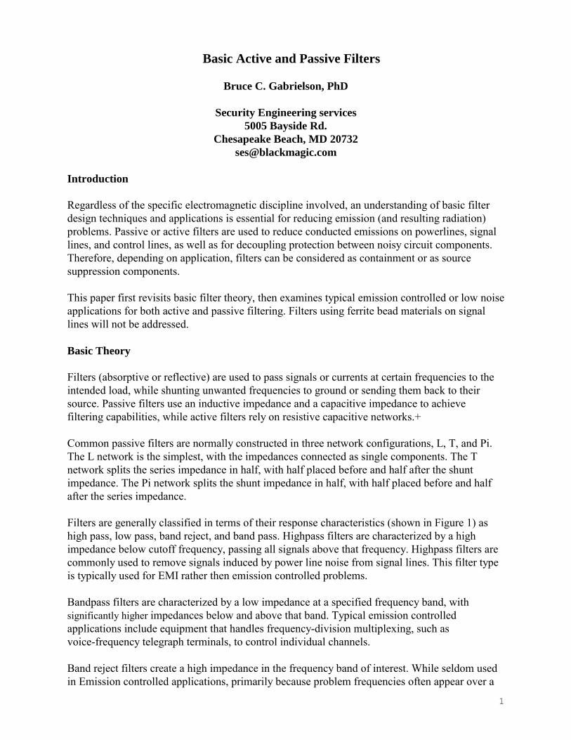
1 Basic Active and Passive Filters Bruce C. Gabrielson, PhD Security Engineering services 5005 Bayside Rd. Chesapeake Beach, MD 20732 [email protected] Introduction Regardless of the specific electromagnetic discipline involved, an understanding of basic filter design techniques and applications is essential for reducing emission (and resulting radiation) problems. Passive or active filters are used to reduce conducted emissions on powerlines, signal lines, and control lines, as well as for decoupling protection between noisy circuit components. Therefore, depending on application, filters can be considered as containment or as source suppression components. This paper first revisits basic filter theory, then examines typical emission controlled or low noise applications for both active and passive filtering. Filters using ferrite bead materials on signal lines will not be addressed. Basic Theory Filters (absorptive or reflective) are used to pass signals or currents at certain frequencies to the intended load, while shunting unwanted frequencies to ground or sending them back to their source. Passive filters use an inductive impedance and a capacitive impedance to achieve filtering capabilities, while active filters rely on resistive capacitive networks.+ Common passive filters are normally constructed in three network configurations, L, T, and Pi. The L network is the simplest, with the impedances connected as single components. The T network splits the series impedance in half, with half placed before and half after the shunt impedance. The Pi network splits the shunt impedance in half, with half placed before and half after the series impedance. Filters are generally classified in terms of their response characteristics (shown in Figure 1) as high pass, low pass, band reject, and band pass. Highpass filters are characterized by a high impedance below cutoff frequency, passing all signals above that frequency. Highpass filters are commonly used to remove signals induced by power line noise from signal lines. This filter type is typically used for EMI rather then emission controlled problems. Bandpass filters are characterized by a low impedance at a specified frequency band, with significantly higher impedances below and above that band. Typical emission controlled applications include equipment that handles frequency-division multiplexing, such as voice-frequency telegraph terminals, to control individual channels. Band reject filters create a high impedance in the frequency band of interest. While seldom used in Emission controlled applications, primarily because problem frequencies often appear over a
Transcript of Basic Active and Passive Filters - Semantic Scholar · source. Passive filters use an inductive...
1
Basic Active and Passive Filters
Bruce C. Gabrielson, PhD
Security Engineering services 5005 Bayside Rd.
Chesapeake Beach, MD 20732 [email protected]
Introduction Regardless of the specific electromagnetic discipline involved, an understanding of basic filter design techniques and applications is essential for reducing emission (and resulting radiation) problems. Passive or active filters are used to reduce conducted emissions on powerlines, signal lines, and control lines, as well as for decoupling protection between noisy circuit components. Therefore, depending on application, filters can be considered as containment or as source suppression components. This paper first revisits basic filter theory, then examines typical emission controlled or low noise applications for both active and passive filtering. Filters using ferrite bead materials on signal lines will not be addressed. Basic Theory Filters (absorptive or reflective) are used to pass signals or currents at certain frequencies to the intended load, while shunting unwanted frequencies to ground or sending them back to their source. Passive filters use an inductive impedance and a capacitive impedance to achieve filtering capabilities, while active filters rely on resistive capacitive networks.+ Common passive filters are normally constructed in three network configurations, L, T, and Pi. The L network is the simplest, with the impedances connected as single components. The T network splits the series impedance in half, with half placed before and half after the shunt impedance. The Pi network splits the shunt impedance in half, with half placed before and half after the series impedance. Filters are generally classified in terms of their response characteristics (shown in Figure 1) as high pass, low pass, band reject, and band pass. Highpass filters are characterized by a high impedance below cutoff frequency, passing all signals above that frequency. Highpass filters are commonly used to remove signals induced by power line noise from signal lines. This filter type is typically used for EMI rather then emission controlled problems. Bandpass filters are characterized by a low impedance at a specified frequency band, with significantly higher impedances below and above that band. Typical emission controlled applications include equipment that handles frequency-division multiplexing, such as voice-frequency telegraph terminals, to control individual channels. Band reject filters create a high impedance in the frequency band of interest. While seldom used in Emission controlled applications, primarily because problem frequencies often appear over a

2
large range of harmonics, they can be employed in selected applications involving a fundamental circuit resonant frequency, or in special RED/BLACK interface situations.
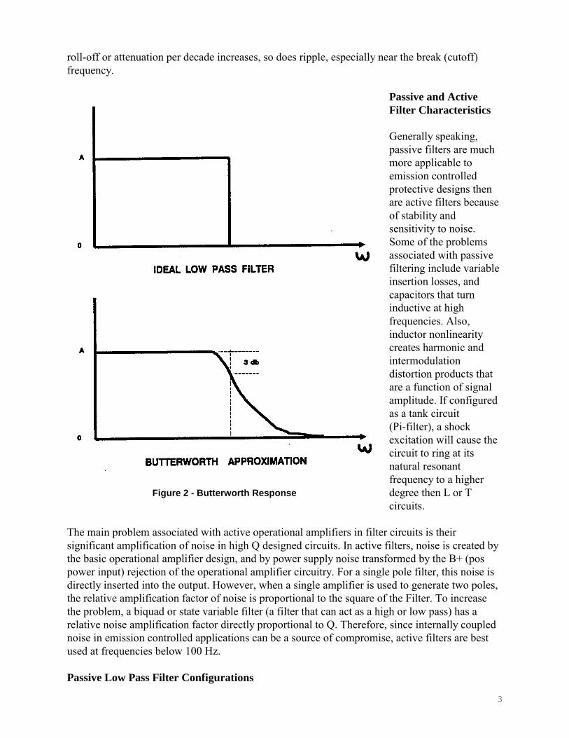
For most emission controlled powerline and signal line applications, low pass filters are normally employed. This filter type passes the signal or current below a specified frequency and attenuate all signals above that point. Since problem signals often appear as harmonics well above their fundamental RED line frequency, and since modulation schemes can create problem signals on carriers existing at frequencies significantly higher then the Red line source, low pass filters are most commonly employed for emission control. For low pass filters, a second classification relates to the roll-off characteristics or "steepness" of the band rejection curve. The three primary response curves relate to Butterworth, Tchebycheff, and Elliptic type filters as shown in Figure 2. Again, since a smooth response is usually preferred in emission controlled applications, and also due to the simplicity of manufacturing and design with few components, Butterworth type filters are commonly used in emission controlled applications. Looking ar the response characteristics of the Butterworth filter in Figure 2, notice the curve is exceedingly flat near zero frequency, and very high attenuation is experienced at higher frequencies. However, the relatively poor roll-off response near cutoff compared to other filter types is the primary reason special purpose bandpass elliptic filters are sometimes used. As
Figure 1 - Filter Response Characteristics
3
roll-off or attenuation per decade increases, so does ripple, especially near the break (cutoff) frequency.
Passive and Active Filter Characteristics Generally speaking, passive filters are much more applicable to emission controlled protective designs then are active filters because of stability and sensitivity to noise. Some of the problems associated with passive filtering include variable insertion losses, and capacitors that turn inductive at high frequencies. Also, inductor nonlinearity creates harmonic and intermodulation distortion products that are a function of signal amplitude. If configured as a tank circuit (Pi-filter), a shock excitation will cause the circuit to ring at its natural resonant frequency to a higher degree then L or T circuits.
The main problem associated with active operational amplifiers in filter circuits is their significant amplification of noise in high Q designed circuits. In active filters, noise is created by the basic operational amplifier design, and by power supply noise transformed by the B+ (pos power input) rejection of the operational amplifier circuitry. For a single pole filter, this noise is directly inserted into the output. However, when a single amplifier is used to generate two poles, the relative amplification factor of noise is proportional to the square of the Filter. To increase the problem, a biquad or state variable filter (a filter that can act as a high or low pass) has a relative noise amplification factor directly proportional to Q. Therefore, since internally coupled noise in emission controlled applications can be a source of compromise, active filters are best used at frequencies below 100 Hz. Passive Low Pass Filter Configurations
Figure 2 - Butterworth Response
4
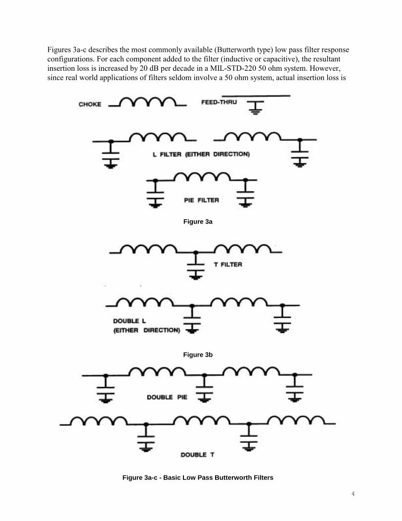
Figures 3a-c describes the most commonly available (Butterworth type) low pass filter response configurations. For each component added to the filter (inductive or capacitive), the resultant insertion loss is increased by 20 dB per decade in a MIL-STD-220 50 ohm system. However, since real world applications of filters seldom involve a 50 ohm system, actual insertion loss is
Figure 3a-c - Basic Low Pass Butterworth Filters
Figure 3a
Figure 3b

5
sometimes calculated to determine if the filter selected will have any effect at all on the problem signal. To determine the performance of a manufactured filter relative to an "other then 50 ohm" system, Figure 4 from Murata Erie (1) provides transfer impedance values which can be used to calculate actual responses. The equation for insertion loss (IL) is: where Zs is the source impedance Zl is the load impedance Z12 is the transfer impedance The transfer impedance is taken from the graph based on the insertion loss specified for the filter in a 50 ohm system. In addition to impedance matching characteristics, each filter has unique characteristics related to the internal resistance and inductance of its capacitor(s), and the parasitic capacitance of its inductor(s). The "C" feed-through filter of Figure 3a is a low impedance filter very efficient for low voltage applications, and/or when both source and load impedances are high. Attenuation for this type of filter is generally between 20 to 40 dB at medium frequencies of around 150 KHz, reducing its usage in most emission controlled applications. The "Pie section of Figure 3a is a low impedance filter used where both source and load impedances are high. Being the most commonly used filter in all applications, it is also one of the most efficient filter types for meeting any voltage and insertion loss requirement.
( )
+=
ls
ls
ZZZZZdBIL
12
1log20)(
Figure 4 - Insertion Loss vs. Transfer Impedance (50 ohm System)

6
The "L� section (Figure 3a) is used on high impedance noise sources and low impedance lines. It is also sometimes used when an output monitoring line is required for a sensitive signal line located inside the Red section of a box. So far as applications for direct filtering of a signal line is concerned, the filter will resonate when shocked with transient noise at selected frequencies, producing dips in the filters resonance curve. Therefore, it is seldom used in direct emission controlled emission control applications. The �T" section (Figure 3b) is used where both the source and the load impedances are low. The filter is very effective in reducing transient type interference since it eliminates ringing, and is normally recommended for circuit interrupting devices. Table 1 provides the consolidated selection criteria for each filter type.
Table 1 – I/O Impedance and Selection Criteria High Input/High Output Impedance
Feed Through Pie Double Pie
High Input/Low Output Impedance
L (C first) Double L (C first)
Low Input/High Output Impedance
L (L first) Double L (L first)
Low Input/Low Output Impedance Choke T Double T
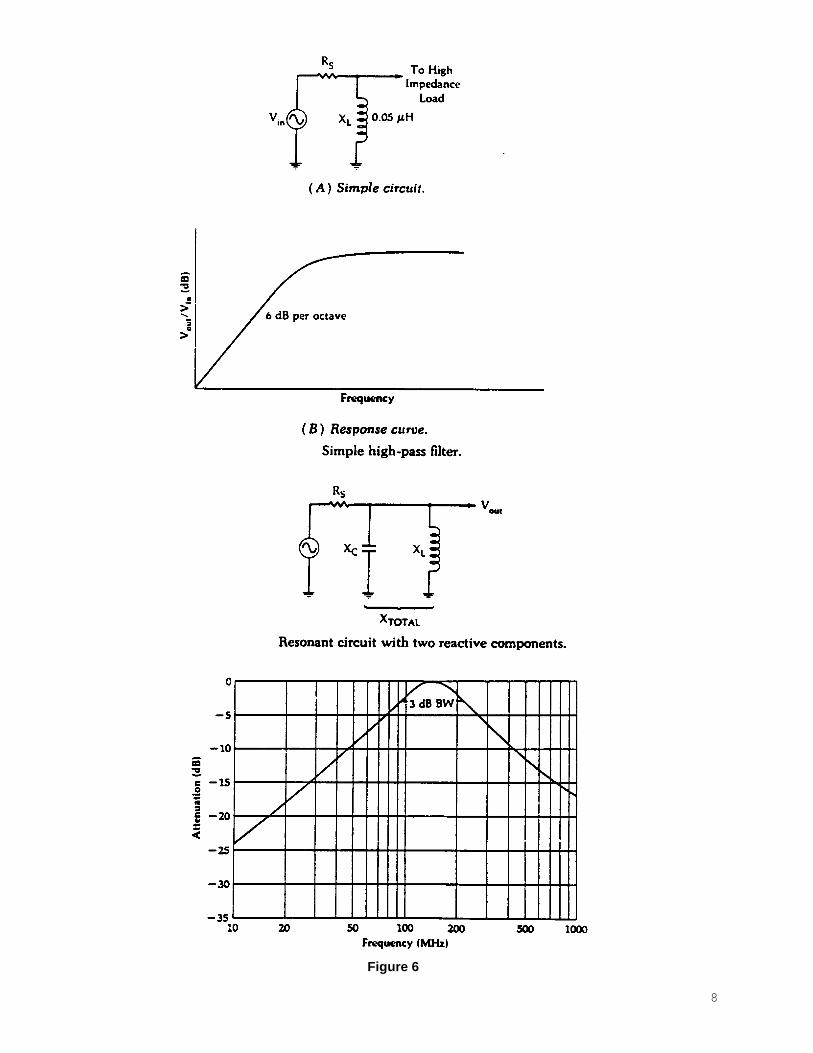
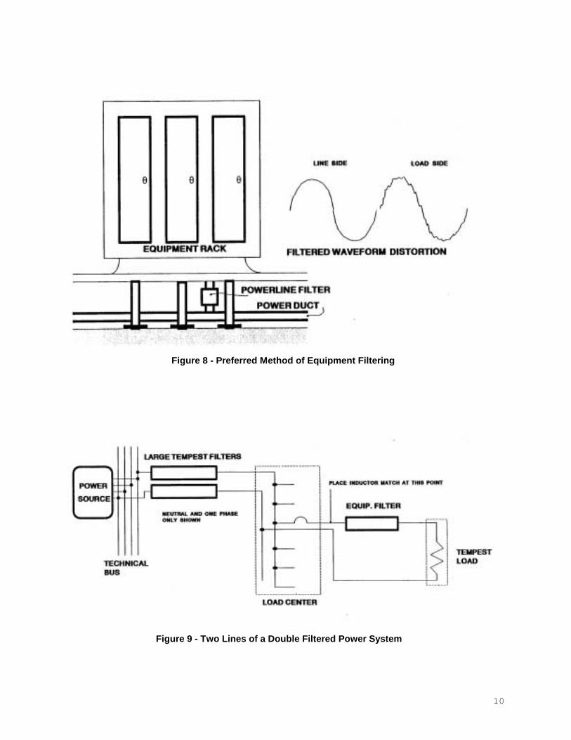
Figure 5 and 6 provide insertion loss characteristics and response equations for typical RC, RL, and LC type circuits. Figure 7 is an example of a series to parallel transformation of an RL circuit. Since custom made filters are expensive, most engineers will usually specify available off-the-shelf filters. Basic Powerline Filters Emission controlled powerline filters can be used in both box and system level applications. The preferred choice for installation is at the equipment level rather than filtering the source of the power at the first service disconnect such as the condition depicted in Figure 8. Bulk facility filtering the power system has the disadvantage of requiring filter selection based on load, with physically massive filters necessary to achieve adequate low frequency responses under significant loads. In no case should a combination of bulk and individual powerline filtering be used on the same equipment. The combination filter can have response characteristics significantly different then the filters used individually. When additional series Pi filters are used in facility applications, such as in the case where two isolated shielded rooms are located next to each other, an air core inductor should be mounted on the top of each metal room in series between the source power filters, and each room filter to prevent miss-match. A double filtered power system and a matched filter system is shown in Figure 9.
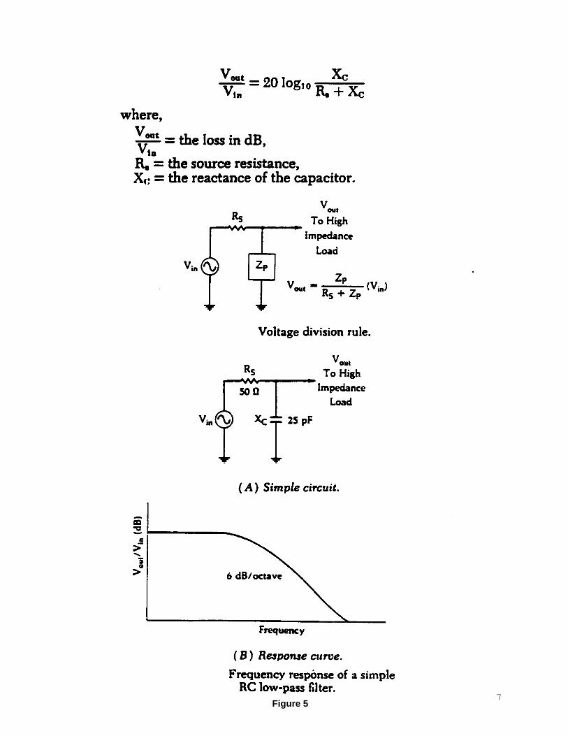
7Figure 5
8
Figure 6

9
Figure 7 - Series to Parallel Conversion Example
10
Figure 8 - Preferred Method of Equipment Filtering
Figure 9 - Two Lines of a Double Filtered Power System
11
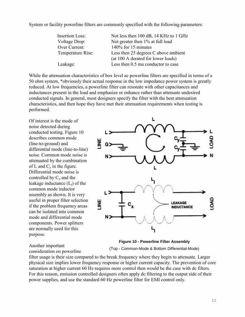
System or facility powerline filters are commonly specified with the following parameters: Insertion Loss: Not less then 100 dB, 14 KHz to 1 GHz Voltage Drop: Not greater then 1% at full load Over Current: 140% for 15 minutes Temperature Rise: Less then 25 degrees C above ambient (at 100 A derated for lower loads) Leakage: Less then 0.5 ma conductor to case While the attenuation characteristics of box level ac powerline filters are specified in terms of a 50 ohm system, *obviously their actual response in the low impedance power system is greatly reduced. At low frequencies, a powerline filter can resonate with other capacitances and inductances present in the load and emphasize or enhance rather than attenuate undesired conducted signals. In general, most designers specify the filter with the best attenuation characteristics, and then hope they have met their attenuation requirements when testing is performed. Of interest is the mode of noise detected during conducted testing. Figure 10 describes common mode (line-to-ground) and differential mode (line-to-line) noise. Common mode noise is attenuated by the combination of L and Cy in the figure. Differential mode noise is controlled by Cx and the leakage inductance (Li) of the common mode inductor assembly as shown. It is very useful in proper filter selection if the problem frequency areas can be isolated into common mode and differential mode components. Power splitters are normally used for this purpose. Another important consideration on powerline filter usage is their size compared to the break frequency where they begin to attenuate. Larger physical size implies lower frequency response or higher current capacity. The prevention of core saturation at higher current 60 Hz requires more control then would be the case with dc filters. For this reason, emission controlled designers often apply dc filtering to the output side of their power supplies, and use the standard 60 Hz powerline filter for EMI control only.
Figure 10 - Powerline Filter Assembly
(Top - Common-Mode & Bottom Differential-Mode)

12
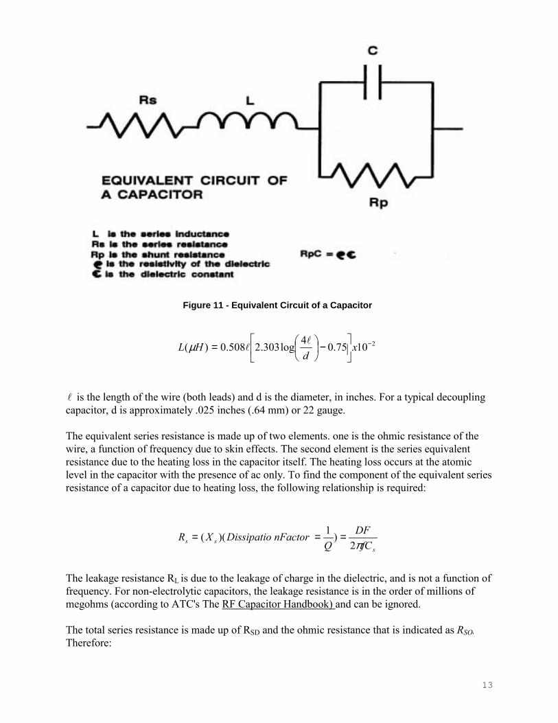
Neutral Filtering Filtering the neutral conductor in a facility is dependent upon the unique physical constraints and of the building and the associated ground system at the location of egress to the controlled area. Measurements of neutral voltage to ground should be made at different points between source and load. If a difference in potential of less then 1 volt is consistently found, then neutral filtering is probably not required. Should a greater then 1 volt potential be identified that is not correctable, neutral filtering is required. If the facility power system is in strict compliance with the criteria in MIL-STD 188-124 and MIL-HDBK 419, then a less then one volt potential should be realized. MIL-HDBK 232A, RED/BLACK Engineering Installation Guidelines, assumes that a dedicated source power (power service transformer and first service disconnect) are physically located within the secure control space (CS). For smaller facilities such as vaults and shielded enclosures, neutral filtering is required. When neutrals of polyphase systems are filtered, the neutral filter must be capable of passing the third harmonic of the combined frequencies of the phases (450 Hz for 3 phase 50 Hz, 540 Hz for 3 phase 60 Hz). Capacitive Filters Capacitance is the ability to store energy. The formula for capacitance is: C= εA(N-1)/ t where C = capacitance ε = dielectric constant A = area of overlap of electrodes N = number of electrodes t = thickness of dielectric As the formula indicates, for higher capacitance, the dielectric constant can be raised (resulting in poorer temperature coefficient), the size of the electrodes can be increased, and/or the number of electrodes can be increased. Each of these techniques results in a larger mechanical size. Decreasing the dielectric thickness also increases capacitance at the expense of lower working voltage thresholds. An equivalent circuit for a capacitor is shown in Figure 11. The equation relating shunt resistance, capacitance, and dielectric resistivity for this circuit is given as: In the figure, L is series inductance, R is series resistance: RL is the leakage resistance, p is resistivity of the dielectric and c is the dielectric constant. Series inductance is calculated from the inductance of a wire formula as:
LRC
ρε=
13
l is the length of the wire (both leads) and d is the diameter, in inches. For a typical decoupling capacitor, d is approximately .025 inches (.64 mm) or 22 gauge. The equivalent series resistance is made up of two elements. one is the ohmic resistance of the wire, a function of frequency due to skin effects. The second element is the series equivalent resistance due to the heating loss in the capacitor itself. The heating loss occurs at the atomic level in the capacitor with the presence of ac only. To find the component of the equivalent series resistance of a capacitor due to heating loss, the following relationship is required: The leakage resistance RL is due to the leakage of charge in the dielectric, and is not a function of frequency. For non-electrolytic capacitors, the leakage resistance is in the order of millions of megohms (according to ATC's The RF Capacitor Handbook) and can be ignored. The total series resistance is made up of RSD and the ohmic resistance that is indicated as RSO, Therefore:
21075.04log303.2508.0)( −
−
= x
dHL l
lµ
sss fC
DFQ
nFactorDissipatioXRπ2
)1)(( ===
Figure 11 - Equivalent Circuit of a Capacitor

14
RSO is a function of frequency, and is calculated as: For copper: Rdc can be found directly from: where: Rdc = dc resistance Rac = ac resistance D = wire diameter in inches f = frequency in hertz l = length in feet A = area in circular mils The temperature coefficient is the change in capacitance that occurs with temperature. In general, most capacitors decrease in capacitance at high temperatures (85 to 125 degrees C) with the effects more noticeable as the dielectric constant increases. Figure 12 shows some typical temperature characteristics of various capacitors in terms of insulation resistance (ρε).
SOSDS RRR +=
=
dc
acdcSO R
RRR
fDRR
dc
ac 960.0=
ARdc
l37.10=
Figure 12 - Temperature Characteristics of RpC

15
Using the equivalent circuit of Figure 11, and omitting RL the capacitive impedance degradation with frequency can be calculated as:
in the s domain In Figure 11 and the above equations: L = series inductance RS = series resistance RSO = series ohmic resistance RSD = equiv. series res. RL = leakage resistance (PD/A) ρ = resistivity As shown in Figure 13, a capacitor has a maximum useable frequency range between 1/RpC and 1/RSC.
Voice Frequency Filters Voice frequency (VF) filters are used in facilities to control audio (300 Hz to 4000 Hz) signals for telephone lines and modems. Low frequency signals are difficult to filter through normal means, and can couple on to carrier signals that exist in the processing equipments pass band region. VF filtering is usually provided at the point of telephone line egress from a Limited Exclusion Area (LEA).
While the use of simple passive low pass filters is satisfactory for common telephone voice band lines, they often cause a problem when employed on quasi-analog modem lines. on modem lines where amplitude modulation or phase-shift keying is used, bandpass filters with a center
sLC
sLRZ S
SS
+
+=
12
LCR1=ω
ωσ js +=
Figure 13 - Impedance of a Capacitor for the Low Loss Case

16
frequency equal to the carrier frequency of the modem are normally required. Active filters are often necessary, but high Q bandpass passive filters will also work to control to potential for higher frequency carrier modulated coupling.
Proper Installation of Passive Filters Filters are supplied in small chassis mountable boxes, tubular bulkhead mounted (feed through), pin filtered connectors, and pc mountable packages. Chassis mountable boxes can be either a box with wires coming out of each end, or they can be intended as a nearly flush surface mounted box that extends into the chassis through a hole. Flush mounted powerline filters normally are the standard power cable, switch, filter and fuze assembly used in many commercial designs. Pin filtered connectors consist of a feed-through capacitor and/or ferrite material formed around each pin in the connector. While only effective at higher frequencies (above 100 MHz), this type of filter has proven very effective at reducing or eliminating signals that appear on interface signal line wiring due to internal radiation. Notice in Figure 14, the filter plate output leads are susceptible to internally radiated signals. Figure 15 shows one example of a box level feed-through filter that requires a solder joint to hold the filter in place. Most applications for box level feed-through filters allow installation using a screw down
Figure 14 - Comparison of Filter Connector and Filter Plate
Figure 15 - Soldered Feed-Thru
17
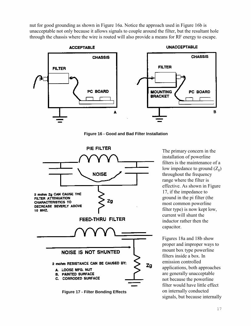
nut for good grounding as shown in Figure 16a. Notice the approach used in Figure 16b is unacceptable not only because it allows signals to couple around the filter, but the resultant hole through the chassis where the wire is routed will also provide a means for RF energy to escape.
The primary concern in the installation of powerline filters is the maintenance of a low impedance to ground (Zg) throughout the frequency range where the filter is effective. As shown in Figure 17, if the impedance to ground in the pi filter (the most common powerline filter type) is now kept low, current will shunt the inductor rather then the capacitor. Figures 18a and 18b show proper and improper ways to mount box type powerline filters inside a box. In emission controlled applications, both approaches are generally unacceptable not because the powerline filter would have little effect on internally conducted signals, but because internally
Figure 16 - Good and Bad Filter Installation
Figure 17 - Filter Bonding Effects

18
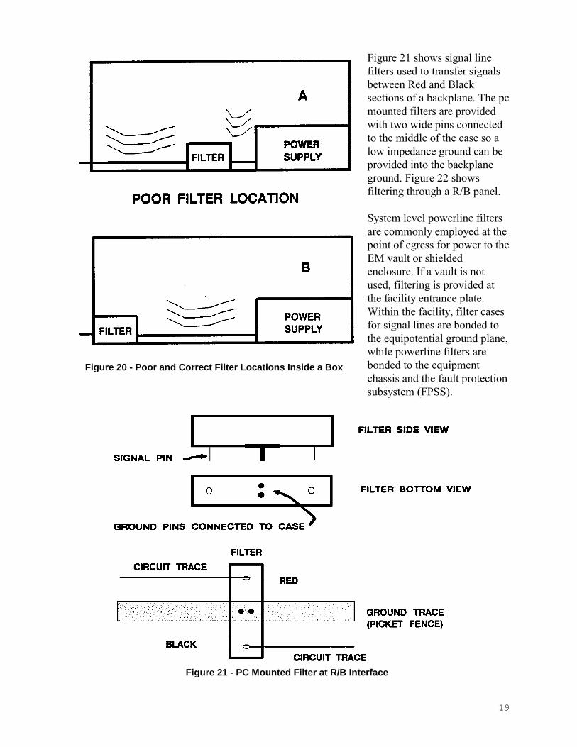
radiated signals can couple around the filter and through the input cable entry to the outside world. For this reason, the type of filter mounting shown in Figure 19 is normally used in commercial emission controlled applications. Notice that in this case, the filter ground is provided by a wide metal flange (ears) connecting the filter to the chassis, with the internal safety ground not being used. Another common mistake in box level powerline filter mounting is to mount the filter close to the power supply, but also well within the equipment at shown in Figure 20a.
As described above, if signals have a coupling access to the raw power side of the filter, they can be easy conducted or radiated outside the box. Therefore, as shown in Figure 20b, Filters should be bulkhead mounted directly to the outside world, and also physically close to the power supply.
Figure 18 - Common Mounting Techniques
Figure 19 - Normal Mounted Filter
19
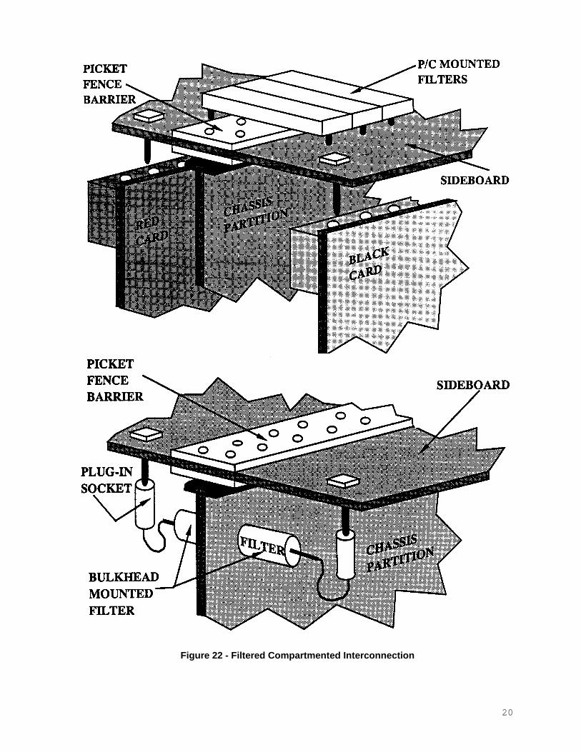
Figure 21 shows signal line filters used to transfer signals between Red and Black sections of a backplane. The pc mounted filters are provided with two wide pins connected to the middle of the case so a low impedance ground can be provided into the backplane ground. Figure 22 shows filtering through a R/B panel. System level powerline filters are commonly employed at the point of egress for power to the EM vault or shielded enclosure. If a vault is not used, filtering is provided at the facility entrance plate. Within the facility, filter cases for signal lines are bonded to the equipotential ground plane, while powerline filters are bonded to the equipment chassis and the fault protection subsystem (FPSS).
Figure 20 - Poor and Correct Filter Locations Inside a Box
Figure 21 - PC Mounted Filter at R/B Interface
20
Figure 22 - Filtered Compartmented Interconnection

21
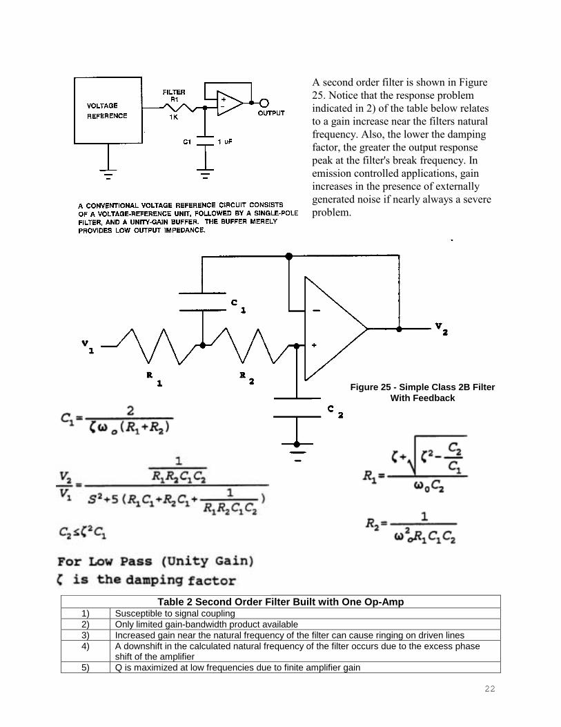
Active Filters Active filters are classified in terms of the number of poles and zeros in their root locus plot. Figure 23 shows first order high and low pass filters and associated design equations. Notice that the big advantages with active low pass filter networks is their ability to increase line impedance using RC rather then LC components. Buffering and impedance matching are major tools in reducing transmission line noise propagation problems. Figure 24 shows a first order filter used as a buffer to provide low output impedance.
High Pass Filter
(K is the Desired Gain)
Figure 23 – High Pass (Above) and Low Pass Filter
22
A second order filter is shown in Figure 25. Notice that the response problem indicated in 2) of the table below relates to a gain increase near the filters natural frequency. Also, the lower the damping factor, the greater the output response peak at the filter's break frequency. In emission controlled applications, gain increases in the presence of externally generated noise if nearly always a severe problem.
Table 2 Second Order Filter Built with One Op-Amp 1) Susceptible to signal coupling 2) Only limited gain-bandwidth product available 3) Increased gain near the natural frequency of the filter can cause ringing on driven lines 4) A downshift in the calculated natural frequency of the filter occurs due to the excess phase
shift of the amplifier 5) Q is maximized at low frequencies due to finite amplifier gain
Figure 25 - Simple Class 2B Filter With Feedback
23
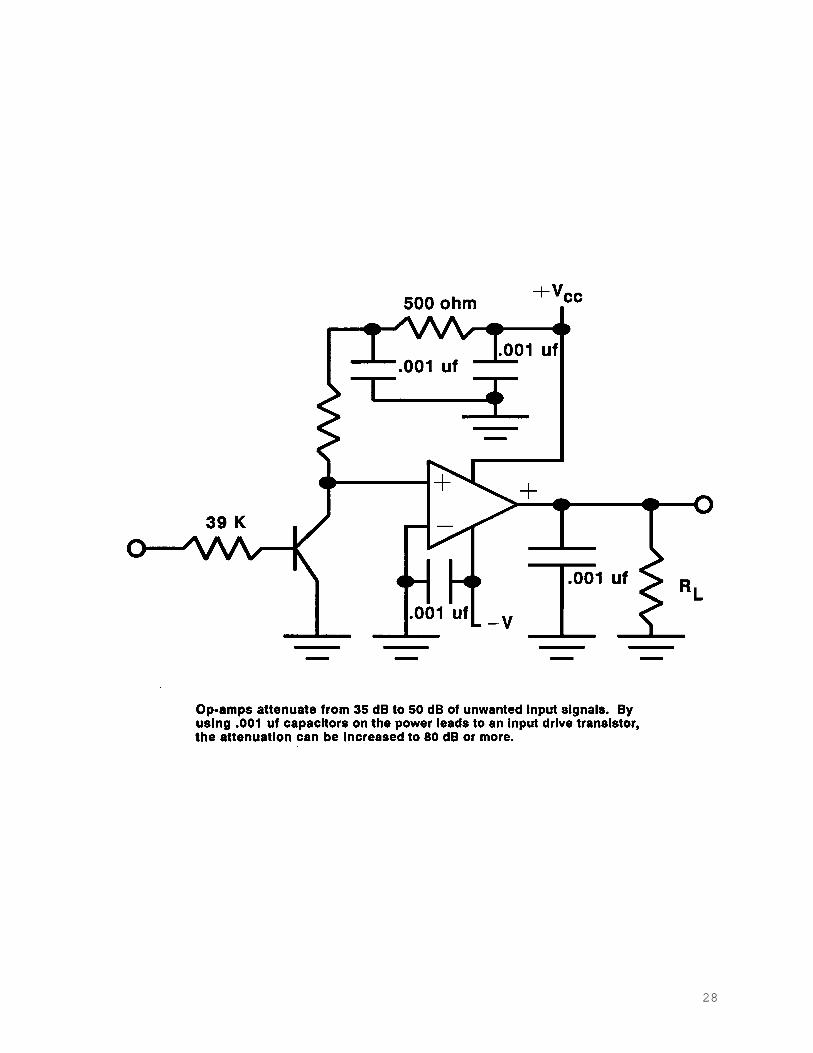
The simple unity gain two-pole (low-pass) filter in Figure 25 can be easily configured using 1% resistors and 5% capacitors to provide a cut-off frequency ranging from hundredths of a hertz to tens of kilohertz. The common approach is to assign a value for R1 = R2 and then calculating for Cl. Arbitrary relationships can cause damping relationship problems and accuracies are greatly effected by what component values are in stock. Also, since high resistance values can drift, and since low resistance values increase input loading, a more acceptable approach for calculating component values takes into account both available component and damping relationship requirements. Low-Pass Filter Design Approach Select a stock value for Cl, selecting a large value if the break frequency is high. Using the equation for low pass unity gain, assign the largest value available which meets the relationship for C2. Having selected Cl and C2, calculate first Rl and then R2 from the equations provided in Figure 25. Resistors are selected from 1% values closest to the calculated numbers. Using the method of selection described, cut-off frequencies can be scaled without changing damping or introducing errors from rounding off values. To change the cut-off frequency, simply divide the values of either R1 and R2 or Cl and C2 by the frequency ratio. Active Filter Board Layout and Location The biggest problem with active filters, and why they are seldom used in emission controlled applications relates to their stability and their susceptibility to signal coupling. As mentioned previously, coupling to the operational amplifier output via conducted signals on power leads are limited only by the amplifier's PSRR. Where active filters find their greatest use in emission controlled applications is when used as line driving circuits.
Provided the circuit is well stabilized, and provided the operational amplifier's power leads are adequately decoupled, filtered, and otherwise protected, the circuit works very well in impedance matching, buffering, and band-width limiting applications. Power input control is sometimes accomplished with three terminal regulators on each supply line close to the op-amp. One problem in line-driver applications relates to off-set voltage. However, many op-amps have offset null capabilities to correct this problem. Look at the specifications for the op-amp before its selection. The op-amp should be located with its associated filter components physically away from sensitive circuitry. To prevent coupling around the filter discrete elements, pc board traces should be run perpendicular (input to output lines) and should be routed on each side of the board with a ground plane in between. Filter Chokes and Linear Inductors Because input filter chokes help reduce the stresses applied to-power supply components, they are commonly used in this type of design. Their use avoids the excessive peak currents typical of
24
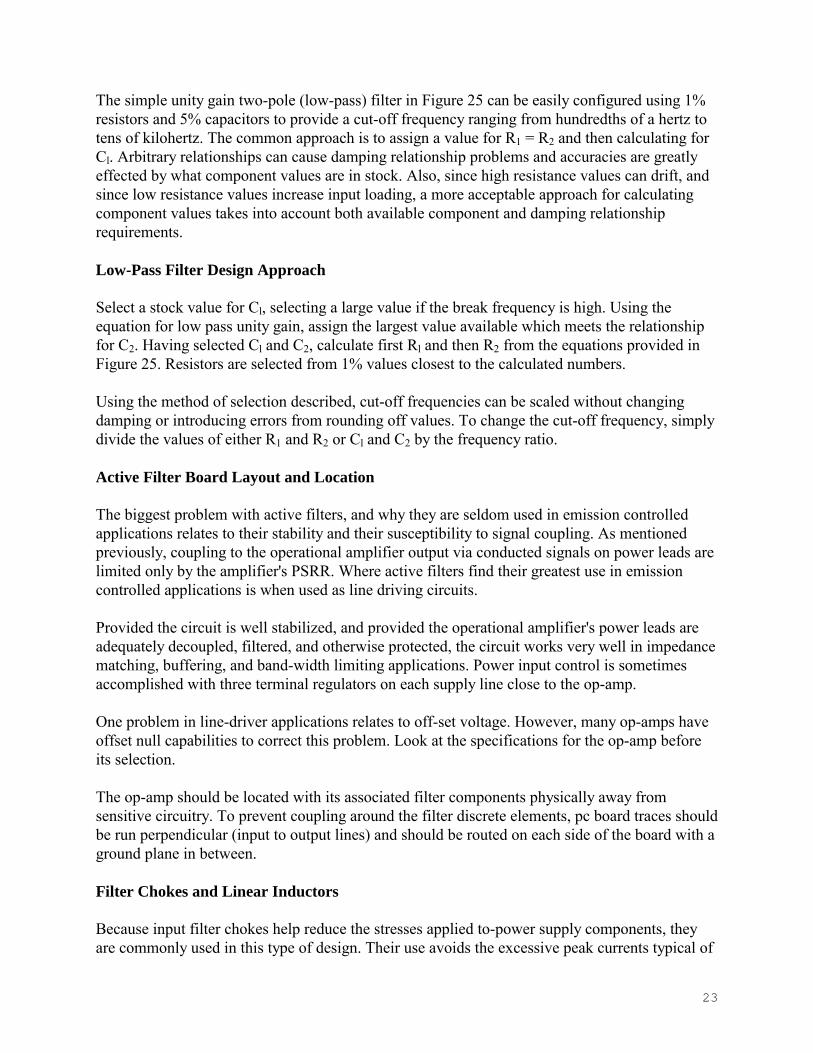
capacitor input filters, thus reducing stress on the power transformer, rectifier circuit, and filter capacitor. Figure 26 shows the location of a choke-input filter within the power system. Linear inductors provide the stability required for filter and tuned circuit applications. They normally consist of a winding placed on an air-gaped ferromagnetic core. All inductors of this type exhibit a maximum Q at some frequency, as shown in Figure 27, and might therefore cause a problem if they are intended to be used where a significant number of noise signals exist over a greatly varying frequency range.
Practical Multiple Applications A constant R filter is sometimes needed in emission controlled applications to eliminate unwanted signals at a Red/Black interface on an analog line. The filter, shown in Figure 28, basically acts as a resonant bandpass circuit to selectively pass the intended signal, while at the same time loading the line in its characteristic impedance. Notice the similarities between this circuit and the typical bandbass circuit of Figure 29.
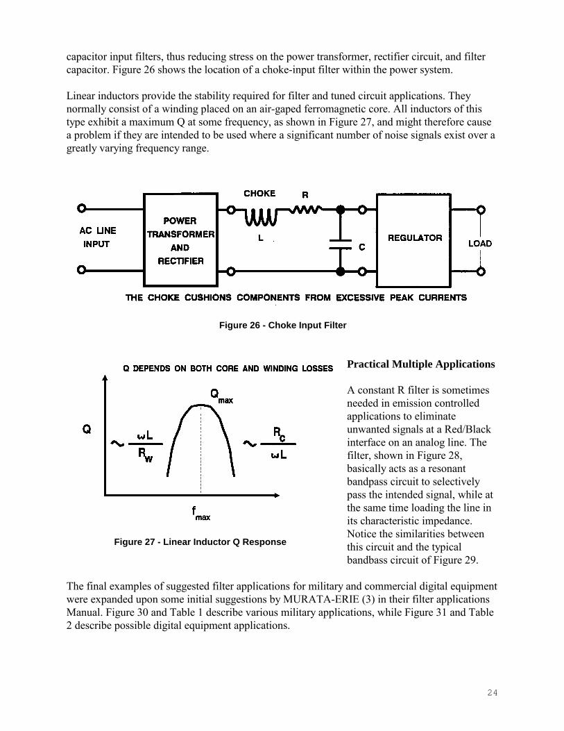
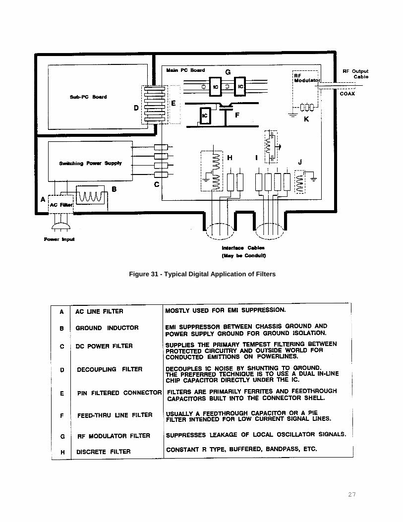
The final examples of suggested filter applications for military and commercial digital equipment were expanded upon some initial suggestions by MURATA-ERIE (3) in their filter applications Manual. Figure 30 and Table 1 describe various military applications, while Figure 31 and Table 2 describe possible digital equipment applications.
Figure 26 - Choke Input Filter
Figure 27 - Linear Inductor Q Response

25
References 1. Gabrielson B.C., and Walter, R.L., An EMC Designers Guide to Operational Amplifiers, ITEM, 1986. 2. Wallace, A., R.F.I. Power Line Filters, Curtis Industries, Inc., 1987. 3. Gerke, D.D., and Kimmel, W.D., Interference Control in Digital Circuits, EMC EXPO 87, San Diego, CA., June, 1987. 4. RED/BLACK Engineering-Installation Guidelines, MIL-HDBK-232A, 20 March, 1987. 5. EM Filter Application Annual, Catalog No. 61-08, Murate Erie North America, Inc., Trenton, Ontario, 1986. 6. Lindquist, C.S., Active Network Design with Signal Filtering Applications, Steward and Sons, Long Beach, CA, 1977. 7. Miller, R., Kusko, A., and Knutrud, T., Filter Chokes and Linear Inductors - The Design Rules Differ, EDN, Nov. 5, 1976. 8. The R.F. Capacitor Design Handbook, ATC.
Figure 28 - Ywo Section Constant R Filter
Figure 29 - Bandpass Filter
26
Figure 30 - Military Applications
27
Figure 31 - Typical Digital Application of Filters
28
29
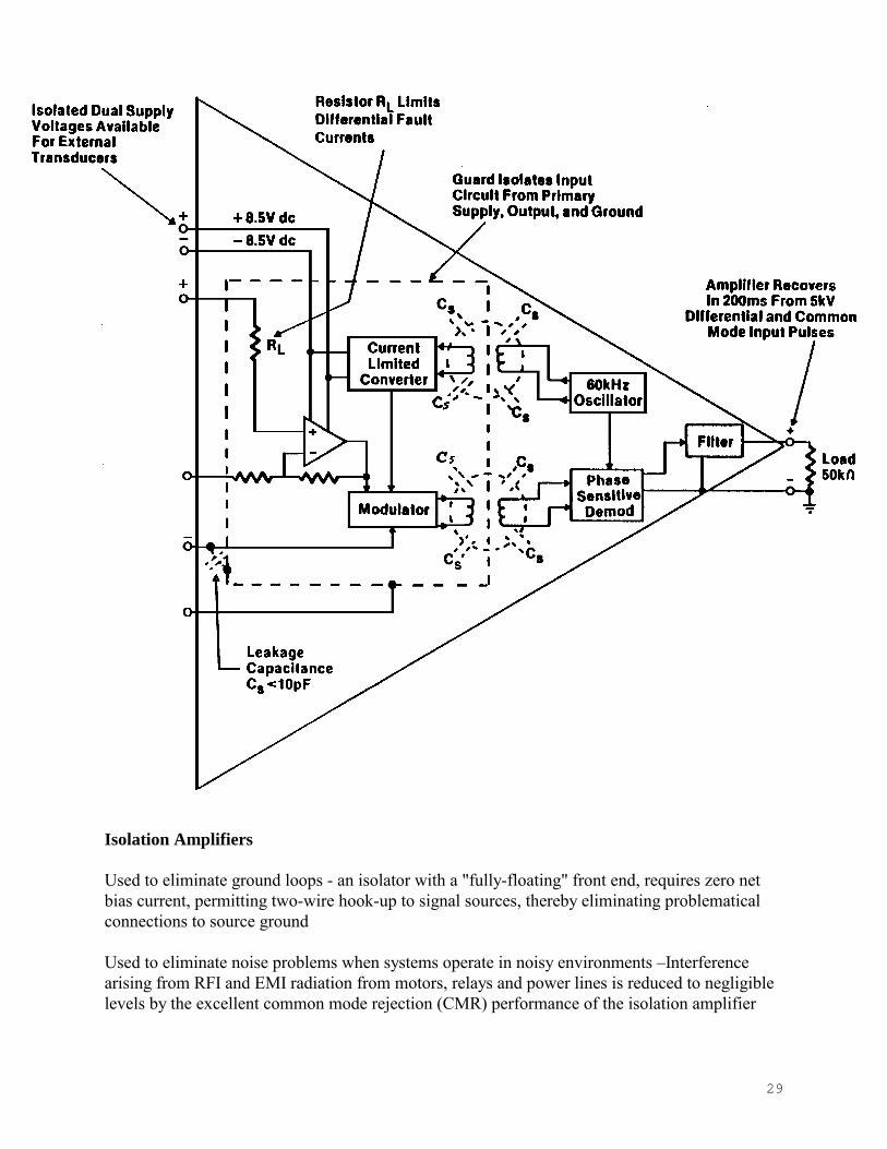
Isolation Amplifiers Used to eliminate ground loops - an isolator with a "fully-floating" front end, requires zero net bias current, permitting two-wire hook-up to signal sources, thereby eliminating problematical connections to source ground Used to eliminate noise problems when systems operate in noisy environments �Interference arising from RFI and EMI radiation from motors, relays and power lines is reduced to negligible levels by the excellent common mode rejection (CMR) performance of the isolation amplifier


![[Vol.ii]Microwave Filters, Impedance-Matching Networks, And Coupling Structures](https://static.fdocuments.in/doc/165x107/55cf8617550346484b9437b3/voliimicrowave-filters-impedance-matching-networks-and-coupling-structures.jpg)