Background - WisTrans: Wisconsin Transportation Center
108
INCORPORATING TOLL PRICING POLICY INTO A MICROSIMULATION MODEL FOR LONG-DISTANCE FREIGHT TRANSPORTATION University of Wisconsin – Milwaukee Paper No. 11-2 National Center for Freight & Infrastructure Research & Education College of Engineering Department of Civil and Environmental Engineering University of Wisconsin, Madison Authors: Qinfen Mei and Alan J. Horowitz Center for Urban Transportation Studies University of Wisconsin – Milwaukee Principal Investigator: Alan J. Horowitz Professor, Civil Engineering and Mechanics Department, University of Wisconsin – Milwaukee May 11, 2011
Transcript of Background - WisTrans: Wisconsin Transportation Center
INCORPORATING TOLL PRICING POLICY INTO A M ICROSIM ULATION M ODEL FOR LONG-DISTANCE FREIGHT TRANSPORTATION University of Wisconsin – Milwaukee Paper No. 11-2
National Center for Freight & Infrastructure Research & Education College of Engineering Department of Civil and Environmental Engineering University of Wisconsin, Madison
Authors: Qinfen Mei and Alan J. Horowitz Center for Urban Transportation Studies University of Wisconsin – Milwaukee Principal Investigator: Alan J. Horowitz Professor, Civil Engineering and Mechanics Department, University of Wisconsin – Milwaukee May 11, 2011

Incorporating Toll Pricing Policy into a Microsimulation Model for Long-Distance Freight Transportation Abstract: Many public policies have been enacted by policy makers and these policies have affected or could affect the freight transportation system. Carriers need to minimize costs to maximize the profits and they often need to deliver the goods to the receivers by a specific time, so toll pricing policy has unpredictable effects on trucker routing decisions. Most freight models in the past have considered only travel time as the path building criterion. This working paper proposes to extend the existing MVFC (Mississippi Valley Freight Coalition) microsimulation model to a new model with the capability of incorporating the toll pricing policy into its traffic assignment step. For dynamic traffic assignments in rural areas, long distance truck drivers usually have a required period of resting after the driving limit. Thus, this paper will also consider the truck driver Hour-of-Service rules in the MVFC model.
One of the key aspects of this paper is the estimation of values of time especially for different commodities and truck classes. The literature review reveals that there are no studies done for values of time by commodity by truck class in the Mississippi valley region or elsewhere. Thus, a truck cost model developed by Hussein (2010) is modified to calculate truck costs for two scenarios: Scenario One (distance-based costs) and Scenario Two (time-based costs) by changing some input data. Then, a linear regression analysis is performed to estimate values of time and per-mile cost for five commodities and two truck classes for each scenario. By using values of time the collected tolls (in dollars) are converted to “extra times” (in minutes). Also, distances are converted to the units of time by using a distance weight, also obtained from the linear regressions.
Three runs with different assumptions on the MVFC network were performed for the case of three industrial commodities assigned using parameters for motor vehicle parts. The comparisons from one run to the other revealed that in response to tolls, truck drivers change their routes when the impedance of the original route exceeds the alternative route’s impedance. The comparisons of the simulation results to actual data from ATR stations in the State of Ohio and from counts provided by the Ohio Turnpike Authority suggest that the values of time for motor vehicle parts in Scenario Two are more reliable than those in Scenario One.
INTRODUCTION
Background The rapid development of the American economy means that billion more tons of goods are
transported on the U.S. freight transportation network each year. The freight system has greatly affected the environment and human activities. State and local governments are charged for constructing, maintaining, operating, funding, and regulating the transportation infrastructures and facilities on which much of the freight moves. Federal, state, and local policy makers have enacted many public policies regarding the freight industry. In terms of revenue generating policies fuel taxes are imposed by federal government and states to build, operate, and maintain the highway system for both freight and passenger vehicles. In addition, other user charges, such as tolls may be adopted by some states and some other authorities to finance highways.
These revenue-generating policies have affected the operating costs for shipping a given commodity, so they are of interest to at least two kinds of institutions: carriers and governments. Carriers are the providers of transportation services, meaning they serve both receivers and suppliers; therefore, customer needs come into play when carriers make travel choices. Carriers usually have to follow a schedule and often need to deliver the goods to the receivers by a specific time. In addition, carriers need to minimize the shipping costs to maximize their profits or to remain competitive. Thus, carriers need to make decisions whether to choose alternative routes to avoid tolls when moving the freight. Governments need to evaluate the impacts of truck traffic diversion so as to enact sound transportation policies in the future. Diverted truck traffic will cause congestion, neighborhood, and safety issues on the alternative routes. Also, toll authorities will lose some revenues due to such traffic diversion.
Short distance truck drivers shipping the goods in urban areas usually travel between two locations in exactly the driving time. Long distance truck drivers in rural areas need to have a required period of resting after the driving limit according to the Hour-of-Service (HOS) rules, so a long-distance truck driver usually drives longer to finish his trip than the driving time. Thus, the truck driver HOS rules are an important factor that affects truck routings and truck costs for the long distance shipping. In addition, they are very important to the safety of trucking operations -- both for the safety of truck drivers themselves and for the safety of others sharing the roads with them.
It is especially important to examine the effects of toll pricing on the freight transportation system. The purpose of this working paper is to develop an efficient model for long-distance freight transportation which is able to simulate truck traffic conditions affected by tolls and other road pricing factors.
Definitions of Key Freight Modeling Terms To help better understand the model described in this paper, it is important and useful to
define several terms relative to freight models and describe key features of them.
1. Commodity A commodity is commonly defined as physical substance (such as food, grains, and metals)
which is interchangeable with another product of the same type, and which investors buy or sell, usually through future contracts. The Quick Response Freight Manual defines it as an item traded

in commerce, which usually implies an undifferentiated product competing primarily on price and availability. However, a commodity in travel modeling is defined as a single category of anything of economic value that needs to be transported.
2. Value of Time Value of time is the change in amount of a traveler’s willingness to pay in money for a unit
change in travel time. In transport economics, value of time is the amount of money a user pays to save time or compensate for lost time.
3. Policy A policy is typically described as a principle or rule to guide decisions and achieve rational
outcome(s). In NCFRP Report 6, policy is often used to do with general statements of principles or goals, and specific government actions. A general policy statement made by a government agency that conveys the desire to adopt measures for some particular purposes is called a policy-in-principle. A policy-in-fact includes formal actions done by elected officials or government agencies. Government decisions to adopt taxes and fees are policies of interest to this paper, because, one way or another, such decisions either directly affect behavior of various entities relating to freight carriage or change in some way the environment in which actors in the freight system operate and make decisions (NCFRP 06, 2010).
4. Toll Toll is usually the amount of money charged by some authorities for the permission to
access a road or a bridge. These roads and bridges are called toll roads and toll bridges.
5. Route A route is a sequence of specific individual facilities (such as, sections of roads, railroad
tracks, etc.) that are used to transport freight between the origin and destination on a specific mode (NCHRP 606, 2008).
6. Truck Cost Model Truck cost models are mathematical algorithmsor equations with some parameters used to
estimate the truck costs under different equipment configurations, input prices, and gross vehicle weights.
7. Microsimulation Microsimulation is the imitation of traffic conditions based on individuals’ behavior by using
a simulation model. Microsimulation is often used to evaluate the effects of proposed interventions before they are implemented in the real world.
8. Four – Step Model A four-step model is usually developed to simulate traffic conditions at present or in the
future, which includes trip generation, trip distribution, mode split, and traffic assignment. In the process of this model, trips begin at a trip generation zone, move through a network of links and nodes by mode and end at a trip attraction zone.

Trip generation is the first step in the travel forecasting model. This step estimates how many trips begin or end in each zone by trip purpose based on a function of land uses, household demographics, and other socioeconomic factors. In the freight model, trip generation estimates the productions and attractions of freight movements in tonnage that begin or end in a geographically defined analysis zone, based on the zonal economic characteristics reflected by employment in particular economic sectors and by number of households.
Trip distribution calculates the number of trips going from each origin to each destination in a trip table or matrix. The gravity model is the most common method for performing this allocation of trips. In the freight model, this step distributes freight flows in tonnage and by commodity group on an O-D basis. The primary impedance variables include average travel distance, average travel time, or composite modal travel time.
Mode split determines the percentage of trips between a given origin and destination that use a particular transportation mode. In the freight model, by using the information about relative benefits of the utility of each freight mode, commodity flow tonnages in the O-D tables are factored by modes such as trucks, rail, etc.
Trip assignment is the fourth step in the conventional transportation forecasting model, following trip generation, trip distribution, and mode choice. It concerns where trips between a given origin and destination by a particular mode are assigned to the transportation network. In the freight model, this step forecasts freight volumes on individual links of the modal networks. When allocating the freight trips, the optimum path or sequence of links between all geographic zones are found based on some important impedance variables, such as travel time, distance, and costs.
9. Control Delay Control delay is defined by traffic control systems handbook (FHWA) as the component of
delay that results when a control signal causes a lane group to reduce speed or to stop; it is measured by comparison with the uncontrolled condition. Control delay includes initial deceleration delay, queue move-up time, stopped delay and final acceleration delay.
10. Level of Service (LOS) Level of service (LOS) defined in traffic engineering is a letter designation that describes a
range of operating conditions on a particular type of facility. Letters A through F are used to define six level of service. Level A represents the best level of service which generally describes operating conditions with free flow and very low delay. Level F represents the worst operating conditions.
11. Dynamic Traffic Assignment Dynamic traffic assignment uses a computer program to build paths for the trucks and these
paths can vary depending on the network condition, congestion, new facilities, etc. Key factors that go into building the paths include infrastructure or cargo restrictions, although specific routings are usually selected as a function of cost, travel time, and quality of service (NCHRP 384, 2008). Dynamic traffic assignment can calculate new routes as congestion increases. It can be used for simulating the situation that the users are charged different toll rates at different time of day.

12. Multiclass Traffic Assignment Multiclass traffic assignment usually tracks truck trips separately from passenger vehicles,
so it can treat truck trips separately by truck size.
13. Clock Time Clock time is the current simulation time, which the simulation model keeps track, in
whatever measurement units are suitable for the system being modeled.
14. Extra Time Extra time presents the value of impedance which can be added to links in the simulation
model but it does not affect clock time. For example, tolls and intersection delay can be coded as extra times.
15. Impedance Impedance is a model variable of each road network link, which represents travel time,
distance, cost or a combination of them. Sometimes it is also called “disutility” or “generalized cost”. It usually has units of minutes.
16. Automatic Traffic Recorders (ATRs) Automatic Traffic Recorders (ATRs) are loops in the pavement surface that continuously
and automatically collect long-term traffic volume data.
17. Electronic Toll Collection (ETC) Electronic toll collection allows the automatic in-lane toll collection process to replace the
manual collection process. By using electronic toll collection, drivers do not have to stop and pay cash at a toll booth and toll booth facility operators can improve customer service and satisfaction by speeding the vehicles through the toll plaza.
18. Average Annual Daily Truck Traffic (AADTT) Average annual daily truck traffic (AADTT) is the total volume of truck traffic on a highway
segment for one year, divided by the number of days in the year (QRFM II, 2007).
19. Calibrate Calibration consists of changing values of model input parameters in an attempt to match
field conditions within some acceptable criteria (Melendez, 2010).
20. Validate Validation is checking a model for how well its assumptions, constants, variables and values
fit specific local system and predicts current conditions (Melendez, 2010).

Introduction of Freight Model As mentioned, this paper is attempting to enhance a freight model with the capability of
modeling the effects of tolls and other pricing factors. Before delving into the description of the model, it is important to introduce some information and theories about freight models.
Transportation planners and policy-makers have a great interest in understanding freight activity and have attempted to better incorporate freight into the travel models. However, efforts to develop microsimulation models of freight demand have lagged noticeably behind models for passenger travel, because freight transportation is determined by numerous of factors and modeling freight movements is a very complicated process. Horowitz (2010) mentioned that there are only a few fledging attempts at using the microsimulation for short-distance urban shipping (Hunt, Stefan and Frownlee, 2006; de Jong and Ben-Akiva, 2007; Hunt and Stefan, 2007; Wisetjindawat, et al., 2007; Wang and Holguin-Veras, 2008) and none for long-distance shipping.
One of the most common modeling techniques for travel demand is the traditional four-step model, which is usually used for personal travel. Four-step models have offered a familiar platform and opportunities to share existing network and algorithms for developing a macroscopic approach to simulating freight movements. Truck-based model and commodity-based model are two major types of freight models. The truck-based models (shown in Figure 1) measure the freight transportation in the form of truck movements without consideration of the amount of commodity production and consumption. These models obviously eliminate the mode choice steps since by definition they include only the truck freight mode. The commodity-based models (shown in Figure 2) closely resemble the four-step travel demand model for passengers including generation of shipments, distribution of shipments, mode split allocation of shipments, and the network assignment of the resulting vehicles.
Traffic assignment is the last step of four-step model, which assigns the modal freight trips to the paths identified from the modal network and forecasts freight volumes on individual links of this modal network. The model looks for optimum paths between all geographic zones, and this path is based on impedance factors such as travel time, travel distance, and cost.

FIGURE 1 Truck-based Model (NCHRP606) FIGURE 2 Commodity-based Model (NCHRP606)
Description of MVFC Model (Horowitz, 2010) The traffic assignment model for this paper is a part of the MVFC microsimulation model,
so there is a need to briefly describe the MVFC model.
The Mississippi Valley Freight Coalition (MVFC), a consortium of ten state DOTs, and the Center for Freight Infrastructure Research and Education (CFIRE, a national university transportation center) teamed to develop a microsimulation of freight demand for a 10-state region in the central U.S., even though it is challenging to work on such a large scale. The current MVFC model covers five indicator commodities (corn, soybeans, dairy products, plastics and motor vehicle parts) which are particularly important for the Mississippi Valley region, and trucking is the only mode of interest. MVFC microsimulation involves several complicated processes, during which many random shipments for a given commodity are generated and then randomly assigned to random vehicles which are finally loaded on a road network.
For the road network, the model has adopted the ORNL network containing all major highways in the U.S. and these highways are represented as 112,000 links. The model retains all the details for the ten MVFC states and 100 miles extension of these states, while it reduces the network outside the defined area to interstate highway, only. Eventually, the reduced network has approximately 44,000 links with many attributes retained from the original ORNL network, but only speed and distance on links have been used in the current microsimulation. And also, the information on link capacity within the region is not used because only a fraction of traffic is being simulated.

For the traffic analysis zones which were defined to be consistent with FAF, they were used within the region only for the purpose of tabulating statistics and rough-checking establishment locations. The MVFC model loaded trips from external super-establishments at intersections nearest the mathematical centroid of FAF zones; such intersections were usually interchanges on interstate highways.
To obtain truck volumes on each road, the traffic assignment algorithm inputted a very large set of trip records, each trip being identified by its origin location (longitude and latitude), destination location, start time, and truck type. Traffic assignments are potentially both multiclass (many vehicle classes) and dynamic.
The MVFC microsimulation model for long-distance freight transportation has the capability of addressing many of the public policies related to freight movements (shown on Table 1).

TABLE 1 Public Policies Addressed in the MVFC Microsimulation Model
Policy
Can be Addressed by a Model (Y/N) Model Feature Assessment
1 HOS Rules for Truck Drivers Y
In a dynamic model, average resting time for truck drivers can be added as time interval after a maximum of 11 hours is driven. Average driving time before resting can be added into the model as well. In the current model, 10 hours are assumed as truckers’ resting time and 11 hours are assumed as driving time. It is notable that driver’s resting time affects the model clock time, not the impedance. Resting time can be also used as a factor in the truck cost model but current cost model does not consider it.
Average resting time and driving time can be obtained by survey but it is time- and money- consuming, so a literature review was conducted but there was little data available. Thus, it's not practical to simulate the real average resting time and driving time, so the current model uses the HOS rule limit (10 hours resting after 11 hours driving) for average resting time and driving time. In the truck cost model, most factors are based on distance so the resting time as time interval only has little effect on costs.
2
Truck Speed Limits and Speed Governor Rules
Y
Actual speed should be used on each link, but in current model, speed for each link is inputted by using the speed limit. To deal with intersection delay, extra time is added to each direction of each surface street to account (roughly) for control delay at the ends of those links. Speed is also used within the truck cost model to obtain the value of time.
Actual speed is based on all the traffic including trucks and autos. Trucks consist of empty trucks and trucks loaded with all commodities and wastes. However, it is quite complicated to run the model considering all vehicles so the current model just considers two classes of trucks and up to five commodities (dairy, plastics, motor vehicle parts, corn, and soybeans). Speed limit is used instead of actual speed. In the truck cost model, an accurate speed would give better estimates for value of time.

TABLE 1 Public Policies Addressed in the MVFC Microsimulation Model (Continuation)
Policy
Can be Addressed by a Model (Y/N) Model Feature Assessment
3
Federal Emission Standards for Diesel Engines
Y
To meet the requirements of Federal Emission Standards for Diesel Engines, the total truck costs will be raised by adding the costs for purchasing new trucks, maintenance and operating, and purchasing new equipment. Finally, the raised total truck costs will result in the higher value of time.
Most of the emission reduction technologies cause a slight reduction in fuel economy (NCFRP 06), so it can offset a little of the raised truck costs.
4
Idling Restrictions for Trucks and Locomotives
N
The model is not able to simulate idling time periods, and idling time does not affect driver behavior. Resting time periods are related to idling. Value of time obtained from truck cost model might be affected by equipment for reducing idling.
5 State Truck Route Restrictions
Y Restricted links can be given a very large travel time. However, the current model does not have truck restriction routes.
Our current model is based on the network provided by Oak Ridge National Laboratory, which contains only major road and does not have truck route restrictions.
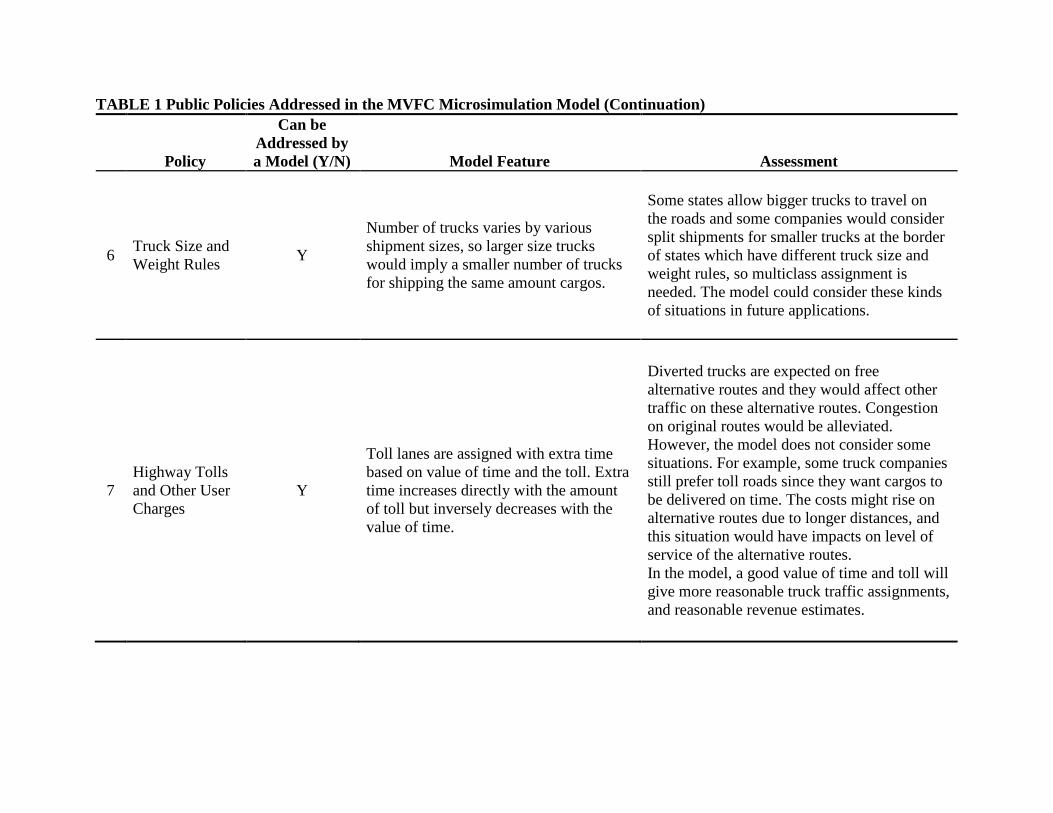
TABLE 1 Public Policies Addressed in the MVFC Microsimulation Model (Continuation)
Policy
Can be Addressed by a Model (Y/N) Model Feature Assessment
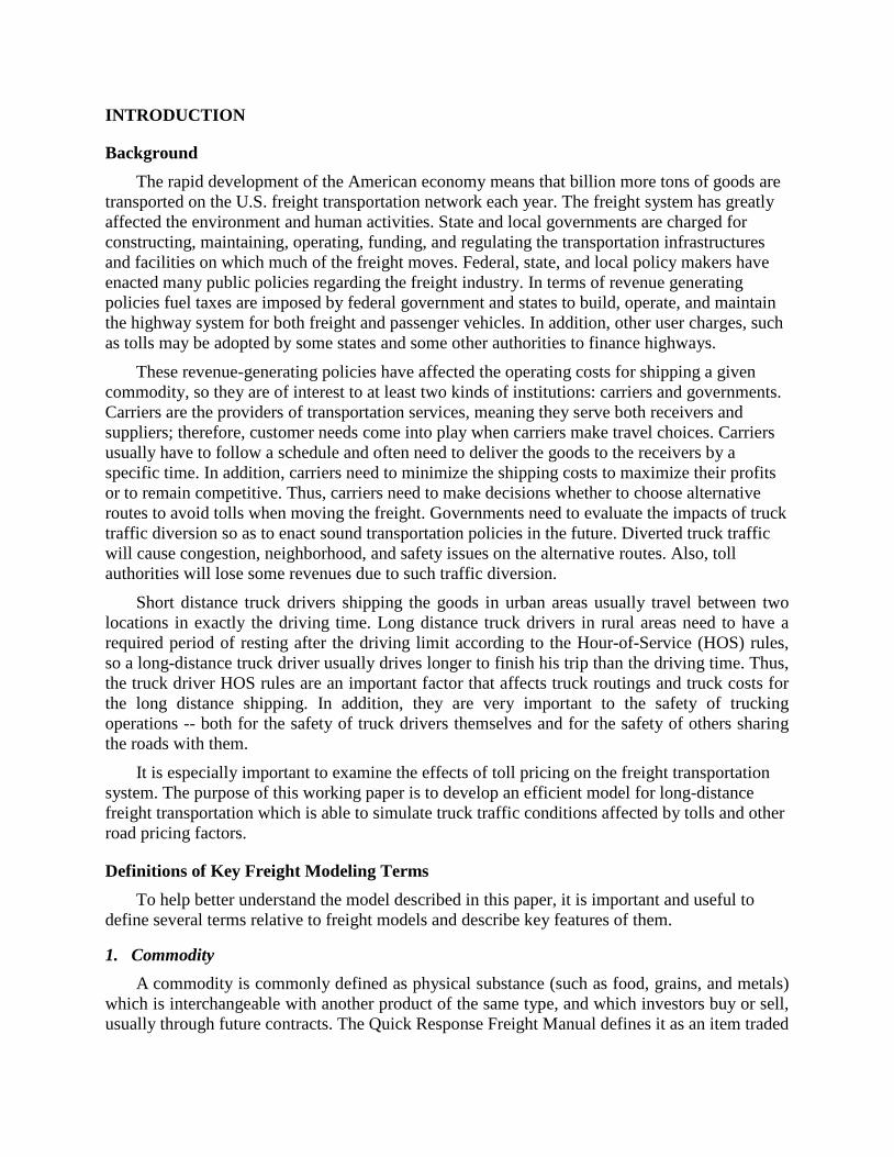
6 Truck Size and Weight Rules Y
Number of trucks varies by various shipment sizes, so larger size trucks would imply a smaller number of trucks for shipping the same amount cargos.
Some states allow bigger trucks to travel on the roads and some companies would consider split shipments for smaller trucks at the border of states which have different truck size and weight rules, so multiclass assignment is needed. The model could consider these kinds of situations in future applications.
7 Highway Tolls and Other User Charges
Y
Toll lanes are assigned with extra time based on value of time and the toll. Extra time increases directly with the amount of toll but inversely decreases with the value of time.
Diverted trucks are expected on free alternative routes and they would affect other traffic on these alternative routes. Congestion on original routes would be alleviated. However, the model does not consider some situations. For example, some truck companies still prefer toll roads since they want cargos to be delivered on time. The costs might rise on alternative routes due to longer distances, and this situation would have impacts on level of service of the alternative routes. In the model, a good value of time and toll will give more reasonable truck traffic assignments, and reasonable revenue estimates.
TABLE 1 Public Policies Addressed in the MVFC Microsimulation Model (Continuation)
Policy
Can be Addressed by a Model (Y/N) Model Feature Assessment
8 Truck Parking Restrictions N
9
Level of Investment in Highway Infrastructure
Y
Level of investment in highway infrastructure will change the capacity of highways, and it will affect the destination choice and mode choice. Current model does not consider it.
Higher level of investment in highway infrastructure has bigger capacity.
10 Hazmat rules Y
Similar to truck route restriction rule, a very large travel time is added to the links on which trucks loaded with hazardous products are restricted to travel. Current model does not consider hazmat.
The road network does not have any routes restricting trucks loaded with hazardous products.
11 Peak Pricing for Port Trucks Y
By using value of time, pricing at peak time for port trucks can be converted to extra time and then the extra time is added on each toll link. Current model does not consider it.
Current model simulates ten states in the Midwest area and port trucks have little effects on traffic congestion, so peak pricing for port trucks is not considered.

TABLE 1 Public Policies Addressed in the MVFC Microsimulation Model (Continuation)
Policy
Can be Addressed by a Model (Y/N) Model Feature Assessment
12 Restrictions on Port Drayage Trucks
N
13 Truck driver background checks
N
14 Restrictions on Locomotive Horns
N
15
Truck electronic onboard recorder rules
N
16 Land use planning requirements
Y
The model can be modified for forecasting future traffic conditions that vary according to land use planning assumptions. Current model does not consider it.
The model can be built for future traffic forecasting when land use for industry is changed by planning, e.g. some factories will move in or move out, new industry area will be built, etc. Current model does not have the capability of addressing it.
17 Property taxes Y Same as 16
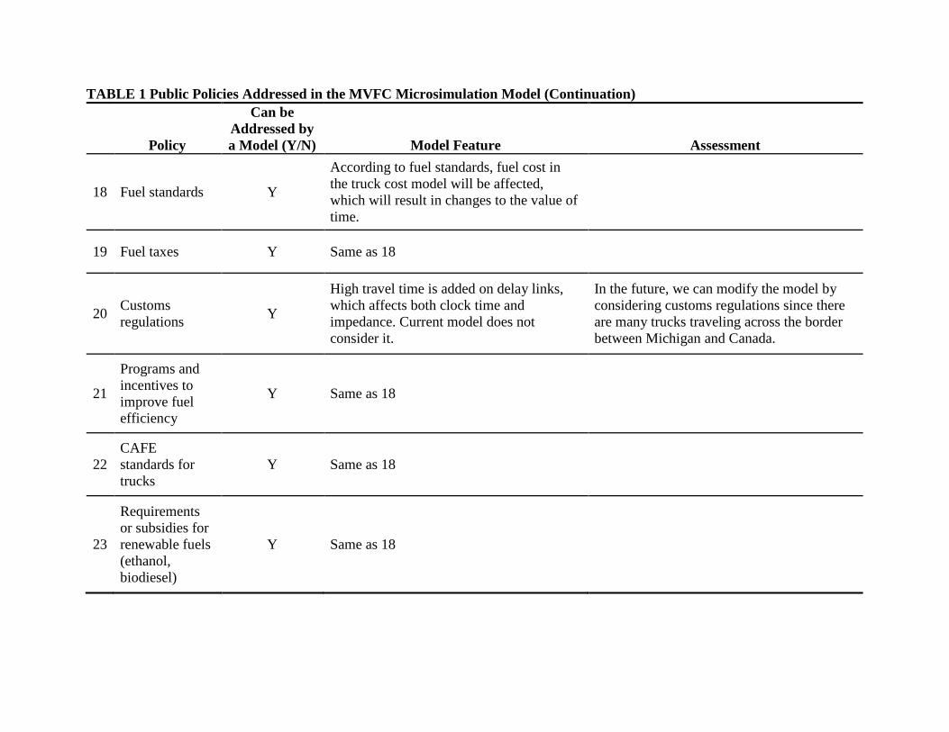
TABLE 1 Public Policies Addressed in the MVFC Microsimulation Model (Continuation)
Policy
Can be Addressed by a Model (Y/N) Model Feature Assessment
18 Fuel standards Y
According to fuel standards, fuel cost in the truck cost model will be affected, which will result in changes to the value of time.
19 Fuel taxes Y Same as 18
20 Customs regulations Y
High travel time is added on delay links, which affects both clock time and impedance. Current model does not consider it.
In the future, we can modify the model by considering customs regulations since there are many trucks traveling across the border between Michigan and Canada.
21
Programs and incentives to improve fuel efficiency
Y Same as 18
22 CAFE standards for trucks
Y Same as 18
23
Requirements or subsidies for renewable fuels (ethanol, biodiesel)
Y Same as 18

TABLE 1 Public Policies Addressed in the MVFC Microsimulation Model (Continuation)
Policy
Can be Addressed by a Model (Y/N) Model Feature Assessment
24
Investment and incentives for alternative fuel infrastructure and vehicles
Y Same as 18
25 Low-carbon-fuel standard Y Same as 18
26 Level of highway funding
Y Same as 9
27 Modal split of funding N
The model is built only for trucks now.
28
Highway operations and maintenance decisions
Y Model can simulate some situations caused by work zones like congestion. Current model does not consider it.
29 Seasonal load limits on highways
Y
Multiclass traffic assignment could be used for different sizes of loads by seasons. Current model does not consider it.
There are no routes limiting seasonal loads for trucks, so current model does not need to simulate it.

Problem Statement To reduce the shipping costs, some truck drivers move to the alternative routes to avoid
tolls. This situation is called truck traffic diversion. However, truck traffic diversion is not easily ascertained by simply looking at how much truck drivers have to pay to access the toll roads and bridges. Travel time and distance of the road segments are usually considered as the two important impedance factors for assigning the traffic on the road network. Most models considered only travel time as the path building criterion. All sources of impedance should be taken into account when simulating truck traffic.
For dynamic traffic assignment in rural areas, long distance truck drivers have to stop their vehicles to have a rest after driving 11 hours according to the HOS rules. There is a need to add the rest periods into the model in order to know the drivers’ total traveling time. Thus, HOS rules can affect the routing of a truck as well as the cost of a haul.
In order to better address the conditions of the truck traffic diversion by using a traffic assignment model in this paper, several research questions need to be considered:
1. How does the MVFC microsimulation model incorporate the public policy (e.g. toll pricing) into the traffic assignment step?
2. What is the relationship among these three impedance factors (travel time, distance, and cost) or is there a function for converting one factor to another?
3. How can we convert the impedance factors in different units into the same units?
4. Where and how can we obtain the value of time by commodity by truck class?
5. Are there some other factors affecting the truck traffic diversion except travel time, distance, and cost?
6. Will the impedance factors affect the truck traffic diversion in a realistic way?
7. What is the average driving time before resting, if a rest is required?
8. What is the average resting time?
The questions above address the purpose of the model. Answering question 2 through question 4 and question 6 is the focus of this paper.

LITERATURE REVIEW
Introduction Many public policies have affected or could affect the whole freight transportation system.
This paper focuses on incorporating the toll pricing policy into the MVFC freight simulation model. Because under this type of policy vehicles are charged for accessing the existing toll roads and bridges; some truck drivers will divert to free alternative roads to seek maximized profits for their trucking firms. Before developing a model to simulate the truck traffic conditions affected by the toll pricing, this chapter will present a literature review of existing studies about some key factors and components of this policy and model.
Toll Pricing The cost for construction and maintenance of highways and bridges is largely covered by the
revenues from fuel taxes and other user charges, especially tolls. Highway and bridge tolls are set by state, local governments and private authorities. The form and the level of tolls would have vital effects on freight system. In particular, tolls are one type of operating costs for trucking firms that can not easily be passed on to customers so they would affect freight (NCFRP 06, 2010). NCFRP 06 (2010) further pointed out that tolls also affect which road the truck drivers choose, and peak period pricing will have some effect on when they use them.
Montana highway reconfiguration study (Montana DOT, 2005) stated that highway toll studies generally focus on the tradeoffs that people make in terms of paying extra cost to reduce travel time (or conversely, their willingness to sit in slower traffic to save tolls). Highway toll studies also reflect driver decisions when they faced these choices (i.e., how drivers value their own time during daily delivery runs). The study also mentioned that the actual form of driver compensation is also different by type of trip. For short-distance drivers who are often paid by the hour, they would gain nothing by paying tolls out of their pockets to save time. For long-distance drivers who are usually paid by a fixed amount per delivery, they have motivation to save time to finish shipments.
Value of Time As pointed out in the Montana highway reconfiguration study, value of time is very
important because it can be used for different purposes. First, it is usually used as one component of the measurement of total economic benefits from alternative highway improvement projects. Second, some studies adopt a value of time to estimate the effects of proposed tolls, new highway connections, highway widening, or lane use policies affecting peak period capacity. Third, there are also some different uses of values of time, such as predicting how travelers would react to tradeoffs between travel time and travel cost in making highway routing decisions, or travel mode choices, or time-of-day travel decisions. Hence, the right way to view the value of time can be different depending on the specific type of user decision being considered and the specific type of application for it.
In this paper, in order to incorporate the highway toll policy into a microsimulation model for freight movements, value of time would be considered as an input to the trip assignment step to convert tolls into equivalent minutes of extra travel time. Besides the toll, distance is another impedance factor for truck drivers to determine which routes to travel on. Value of time, also as one of the parameters affecting the weight in the impedance function for distance relative to

time, will be used to convert the units of distance to the units of time. Thus, the importance for good values for travel time is obvious and a review of earlier work will be very useful.
Studies about Value of Time in US
VOT Obtained from Literature Review To get a reasonable estimate for values of time for trucks, Outwater and Kitchen (PSRC,
2008) conducted a national literature search of observed or estimated truck values of time and this literature search identified a range of $40 per hour to $50 per hour for light, medium and heavy trucks.
Another literature review was also conducted by Outwater and Kitchen, along with Ardussi, Bassok and Rossi (PSRC, 2009) because they needed truck values of time as an input to a trip assignment model whenever tolls are imposed to convert tolls into equivalent minutes of travel time. The sources from literature review are identified as follows:
Smalkowski et al conducted interviews in Minnesota in 2003 using an adaptive stated preference survey to derive a truck value of time of $49 per hour. Surveys were conduced for for-hire, fleet and private trucks.(PSRC, 2009)
Kawamura estimated a value of time for trucks at $28 per hour from stated preference data collected in California in 2000. His research found that for-hire trucks tend to have a higher value of time than private ones and companies that pay drivers hourly wages have higher values of time than those who pay commissions or fixed salary. (PSRC, 2009)
In 2006, FHWA reported that shippers and carriers assign a value to increases in travel time of $25 to $200 per hour, depending on the commodity carried. The value of reliability for trucks is another 50 to 250% higher. (PSRC, 2009)
In 2005, FHWA reported that the delay cost for trucks in bottlenecks was $32 per hour. This value of time was noted as a conservative estimate of value of time from the FHWA Highway Economic Requirements System (HERS). (PSRC, 2009)
Wigan et al estimated $1.30 pallet/hour for urban full truck loads (FTL) and $1.40 pallet/hour for metropolitan multi-drop deliveries based on contextual stated preference (CSP) surveys of Australian shippers. Using an average size of 19 pallets per medium truck and 34 pallets per heavy truck, Wigan et al estimate a range of value of travel time of $25-27 per hour for medium trucks and $44-48 per hour for heavy trucks. This study also estimated a value of reliability at $1.25 for urban FTL and $1.97 for metropolitan multi-drop per 1% reduction. (PSRC, 2009)
Holguin-Veras estimated the necessary conditions for off-hour deliveries to determine the effectiveness of urban freight road pricing in competitive markets. In this research, he found that receivers are likely to experience incremental costs in the range of $14 to $49 per hour of off-hour operation. (PSRC, 2009)
Having found the difficulty of identifying trip decision-makers, the PSRC working group agreed that a reasonable value of time for trucks in the Puget Sound region was $40 per hour for light trucks, $45 per hour for medium trucks, and $50 per hour for heavy trucks, which are

consistent with the results from Outwater and Kitchen (2008) described earlier. From the results of literature review, some studies (Smalkowski et al 2003, Kawamura 2000, FHWA 2005, 2006, Holguin-Veras) presented some meaningful truck values of time but did not specify detailed value of time based on different type of trucks, which have been done by Wiganet and Outwater. However, Wiganet and Outwater did not analyze these values of time according to different type of commodities loaded on trucks.
Killough (2008) has focused on value analysis of truck toll lanes in congested conditions. To make an assessment of the truck toll lane contribution to improve travel time reliability and see how consideration of reliability enhanced the ROI analysis, he assumed a value of $73 per hour for heavy truck and a per-mile truck toll lane cost of $0.86, according to the finding that shippers and carriers value travel time are at $25 to $200 per hour depending on the cargo by the Federal Highway Administration (FHWA). Even though a value of time is observed, the author did not identify truck value of time for different types of commodities. And also, he just gave the value of time for heavy-duty trucks.
Concas and Kolpakov (2009) also conducted a study with the objective to compile and synthesize current and past research on the value of time (VOT) and the value of reliability of time (VOR). A summary table of review work about value of time was provided on Table 2 but there is no study about value of time specific for different commodities and truck classes.

TABLE 2 Summary of Empirical Work (Concas, Kolpakov, 2009) St
udy Sample Size;
Geographic Scale; Data Used
Estimation Process; Relevant Variables
Finding
(Lam
, 200
4)
- Travel data from State route 91 and I-15 in California
- Monte Carlo simulation is applied to scheduling and route choices of individuals to examine and compare the welfare of conventional road expansion policies and value priced projects
- Individual route and scheduling choices are based on the model of Lam (2000)
- Travel choices are interacted in accordance with behavioral rules to produce time savings benefits and scheduling benefits in different scenarios of the study
- While the tolled lanes in value-pricing projects yield the most benefits to commuters with high value of time, free lane users also benefit indirectly from the increased capacity when commuters switch to tolled lanes
- Value priced projects are found to produce consistently larger aggregate benefits in terms of welfare compared to conventional road expansion policies
- Various simulations produce value of time with mean of $9/hour or $21/hour, and standard deviation of $10.50/hour
(Cal
fee
and
Win
ston
, 199
8)
- National Family Opinion survey (mail survey)
- Data covers a random sample of
1,170 automobile commuters from major U.S. metropolitan areas who regularly drove to work
- The analysis estimates automobile commuters’ willingness to pay to save travel time
- Willingness to pay is examined under a variety of travel conditions and assumptions about how toll revenue will be spent
- There is no evidence that commuters willingness to pay depended on how the toll revenue is spent
- Average willingness to pay to reduce travel time was estimated in the range of 14%-26% of the gross hourly wage, with an average of 19% for the entire
sample, and is insensitive to travel conditions
- Travelers are able to adjust to
congestion through their modal,
residential, workplace and departure time choices (this implies that even high income commuters may be unable to benefit substantially from tolls)
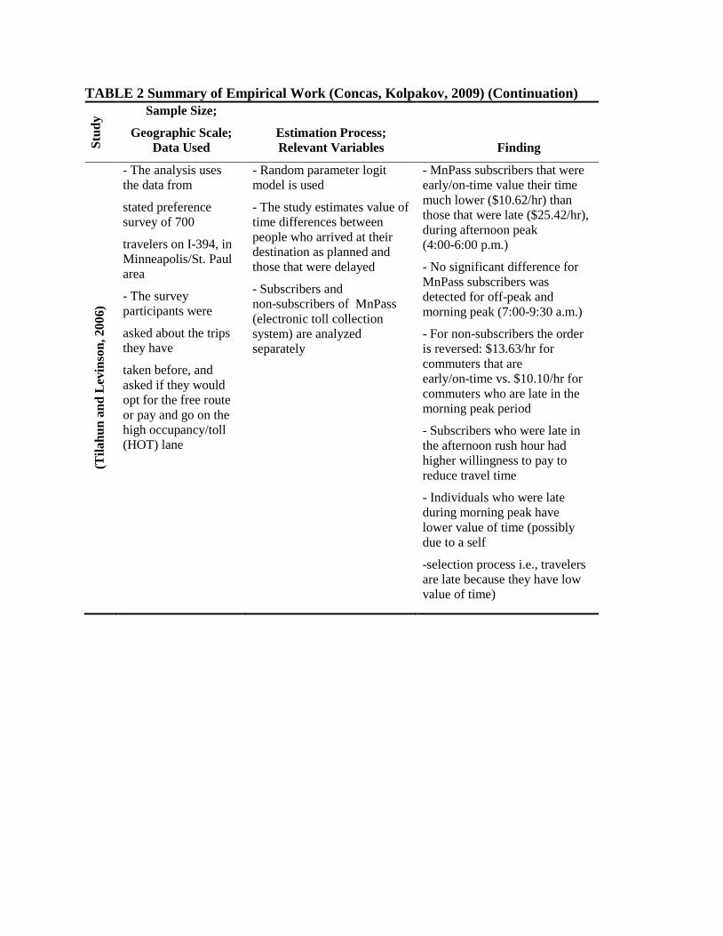
TABLE 2 Summary of Empirical Work (Concas, Kolpakov, 2009) (Continuation) St
udy Sample Size;
Geographic Scale; Data Used
Estimation Process; Relevant Variables Finding
(Tila
hun
and
Levi
nson
, 200
6)
- The analysis uses the data from
stated preference survey of 700
travelers on I-394, in Minneapolis/St. Paul area
- The survey participants were
asked about the trips they have
taken before, and asked if they would opt for the free route or pay and go on the high occupancy/toll (HOT) lane
- Random parameter logit model is used
- The study estimates value of time differences between people who arrived at their destination as planned and those that were delayed
- Subscribers and non-subscribers of MnPass (electronic toll collection system) are analyzed separately
- MnPass subscribers that were early/on-time value their time much lower ($10.62/hr) than those that were late ($25.42/hr), during afternoon peak (4:00-6:00 p.m.)
- No significant difference for MnPass subscribers was detected for off-peak and morning peak (7:00-9:30 a.m.)
- For non-subscribers the order is reversed: $13.63/hr for commuters that are early/on-time vs. $10.10/hr for commuters who are late in the morning peak period
- Subscribers who were late in the afternoon rush hour had higher willingness to pay to reduce travel time
- Individuals who were late during morning peak have lower value of time (possibly due to a self
-selection process i.e., travelers are late because they have low value of time)

TABLE 2 Summary of Empirical Work (Concas, Kolpakov, 2009) (Continuation) St
udy Sample Size;
Geographic Scale; Data Used
Estimation Process; Relevant Variables Finding
(Tse
ng, U
bbel
s and
Ver
hoef
, 200
5)
- Interactive computer-based survey among Dutch commuters, collected during three weeks in June 2004
- Data covered 6,800 working adults who drive to work by car two or more times per week, and who face congestion of 10 or more minutes for at least two times a week
- The analysis empirically estimates travelers’ valuation of travel time, scheduled delay and uncertainty
- Multinomial logit model is used to estimate choices of the motorists
- Socio-economic characteristics controlled: income, education, and arrival/departure time restriction
- The value of time is higher for
travelers when they are late
- Mean value of time for all travelers is 10 Euros/hour ($12.10/hr), and the value of schedule delay late (VSDL) has the mean value of 14 Euros/hour ($16.94/hr)
- Inflexible commuters generally have a higher value of time, schedule delay and uncertainty
- Reliability is valued at roughly half of the value of time (5.3 Euros/hr = $6.41/hr)
- Commuters prefer the car over the public transportation alternative
- People’s aversion to arriving early is increasing non-linearly as their schedule delay early time increases
- Income and the length of commuting trip affect the value of time
VOT Obtained from Some Methods For the value analysis of truck toll lanes in congested condition, Kawamura (2003) used
empirically derived value of time distributions to calculate the perceived benefits from the time savings associated with the use of toll lanes by trucks. The mean values of time for toll lane users and non-users were estimated using Monte Carlo simulations. This study differentiates value of time between for-hire ($28/h) and in-house ($17.6/h) trucks. However, the author did not identify values of time for different types of commodities and different FHWA truck classes.
Kruesi (US DOT, 1997) established consistent procedures to be followed by agencies within the Department of Transportation and evaluated savings or losses of travel time that result from
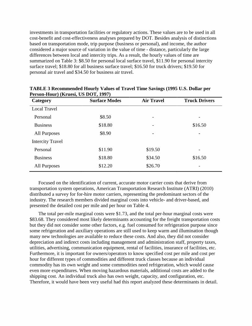
investments in transportation facilities or regulatory actions. These values are to be used in all cost-benefit and cost-effectiveness analyses prepared by DOT. Besides analysis of distinctions based on transportation mode, trip purpose (business or personal), and income, the author considered a major source of variation in the value of time - distance, particularly the large differences between local and intercity trips. As a result, the hourly values of time are summarized on Table 3: $8.50 for personal local surface travel, $11.90 for personal intercity surface travel; $18.80 for all business surface travel; $16.50 for truck drivers; $19.50 for personal air travel and $34.50 for business air travel.
TABLE 3 Recommended Hourly Values of Travel Time Savings (1995 U.S. Dollar per Person-Hour) (Kruesi, US DOT, 1997) Category Surface Modes Air Travel Truck Drivers
Local Travel
Personal $8.50 - -
Business $18.80 - $16.50
All Purposes $8.90 - -
Intercity Travel
Personal $11.90 $19.50 - Business $18.80 $34.50 $16.50
All Purposes $12.20 $26.70 -
Focused on the identification of current, accurate motor carrier costs that derive from
transportation system operations, American Transportation Research Institute (ATRI) (2010) distributed a survey for for-hire motor carriers, representing the predominant sectors of the industry. The research members divided marginal costs into vehicle- and driver-based, and presented the detailed cost per mile and per hour on Table 4.
The total per-mile marginal costs were $1.73, and the total per-hour marginal costs were $83.68. They considered most likely determinants accounting for the freight transportation costs but they did not consider some other factors, e.g. fuel consumed for refrigeration purpose since some refrigeration and auxiliary operations are still used to keep warm and illumination though many new technologies are available to reduce these costs. And also, they did not consider depreciation and indirect costs including management and administration staff, property taxes, utilities, advertising, communication equipment, rental of facilities, insurance of facilities, etc. Furthermore, it is important for owners/operators to know specified cost per mile and cost per hour for different types of commodities and different truck classes because an individual commodity has its own weight and some commodities need refrigeration, which would cause even more expenditures. When moving hazardous materials, additional costs are added to the shipping cost. An individual truck also has own weight, capacity, and configuration, etc. Therefore, it would have been very useful had this report analyzed these determinants in detail.

TABLE 4 Costs per Mile and Costs per Hour for Motor Carriers (ATRI, 2010) Motor Carrier Marginal Expenses Costs Per Mile Costs Per Hour
Vehicle-based
Fuel-Oil Costs 0.634 $33.00
Truck/Trailer Lease or Purchase Payments 0.206 $10.72
Repair and Maintenance 0.092 $4.79
Fuel Taxes 0.062 $3.23
Truck Insurance Premiums 0.06 $3.12
Tires 0.03 $1.56
Licensing and Overweight-Oversize Permits 0.024 $1.25
Tolls 0.019 $0.99
Driver-based
Driver Pay 0.441 $16.59
Driver Benefits 0.126 $6.56
Driver Bonus Payments 0.036 $1.87
Total Marginal Costs $1.73 $83.68
VOT Obtained from Literature Review and Methods A cost benefit study was conducted by Smalkoski, Levinson (2005) to examine the spring
load restriction policy of Minnesota which has been in effect for over 50 years with little consideration given to the cost that it imposes on the freight industry. This cost-benefit analysis required a precise estimate of the value of time for commercial vehicle operators in Minnesota but there is no such an estimate available from previous studies or data (shown on Table 5). Thus, this study conducted interviews by using an adaptive stated preference (ASP) survey to derive an estimate to the nearest dollar. Then a tobit model was fit to the data from the interviews to obtain the estimate for value of time and a mean of $49.42 was found, with a 95% confidence interval from $40.45 to $58.39.

TABLE 5 Summary of Previous Value of Time Studies (Smalkoski, Levinson, 2005)
Authors Year of
Publications Focus Location Adjusted to
2003
Average Value Per
Hour
Haning and McFarland 1963 Truck Operators
$19.57 to $25.42 $22.50
Water et al. 1995 Truck Operators
$6.86 to $38.92 $22.89
Kawamura 1999 Truck Operators
$30.14 $30.14
Brownstone et al. 2003 Automobiles San Diego $30.58 $30.58
Lam and Small 2001 Automobiles California $21.36 $21.36
Adkins et al. 1967 Cargo Vehicles
$25.81 $25.81
Overall Average $25.55
Std. Dev. $4.01
Studies about Value of time in Foreign Countries
VOT Obtained from Literature Review A useful review of studies was also done to analyze value of time by Fowkes (2001). In his
study, Fowkes, Nash and Tweddle (1989) gave values of time per vehicle disaggregated by commodity type and these values have been converted to 1995 monetary values (shown on Table 6).
TABLE 6 Value of Time by Commodity (Fowkes, Nash and Tweddle, 1989) VOT per vehicle
(£/hr) (p/min)
Fertiliser 1.3 2
Cement 4 7
Domestic Appliances 3.2 5
Chocolate 6.5 11
Beer 7.7 13
Oil 7.5 13
Tubes 13 22
Paper products 15 25
Note: £ is the symbol for British pound, p is the symbol for pence.
Victoria Transport Policy Institute (2010) examined the value of travel time, and travel time savings because travel time accounts for one of the largest costs of transportation, and travel time savings are often the primary justification for transportation infrastructure improvements.

Various studies have developed estimates of travel time for different user types and travel conditions in their study. For example, TransFund New Zealand used standard travel time values summarized on Table 7, in which “work travel” involves travel while paid, “Non-work” travel is all personal travel including commuting, and “Congested Premium” is an additional cost for travel in congested conditions.
TABLE 7 Base Values for Vehicle Occupant Time (1998 NZ Dollars per Hour) (Victoria Transport Policy Institute, 2010)
Mode Work Travel Non-Work
Travel Congestion Premium
Car, Motorcycle Driver $21.30 $7.00 $3.50
Car, Motorcycle Passenger $21.30 $5.25 $2.60
Light Commercial Driver $19.25 $7.00 $3.50
Light Commercial Passenger $19.25 $5.25 $2.60
Medium Commercial Driver $15.80 $7.00 $3.50
Medium Commercial Passenger $15.80 $5.25 $2.60
Heavy Commercial Driver $15.80 $7.00 $3.50
Heavy Commercial Passenger $15.80 $5.25 $2.60 Seated Bus Passenger $21.30 $5.25 $2.60
Standing Bus Passenger $21.30 $10.55 $2.60
Pedestrian and Cyclist $21.30 $10.55 N/A
VOT Obtained from Some Methods Wigan, Rockliffe, Thoresen and Tsolakis (2000) applied contextual stated preference (CSP)
methods and the associated multinomial logit models to estimate the value of some factors from an Australian survey of freight shippers using road freight transport in 1998. It was concluded that the estimated value of long-haul freight transport travel time per pallet per hour on intercity routes is at $0.7, while for metropolitan (intra-city) routes it is estimated at $1.3 (Wigan, Rockliffe, Thoresen and Tsolakis, 2000) and these values are shown on Table 8. From these estimates, the authors stated that metropolitan freight travel time is more highly valued than that of intercity freight movements. Furthermore, the author pointed out that the value of multi-drop freight travel time per delivery per hour on strictly metropolitan routes is estimated at $1.4, similar to the metropolitan FTL estimate of $1.3 (shown on Table 8).

TABLE 8 Freight Travel Time: Implicit Unit Values (in 1998 $ AUD) (Wigan, Rockliffe, Thoresen and Tsolakis, 2000) Segment Freight Travel Time Reliability Damage
Inter-capital(FTL) $.66 pallet/hour $2.56 per 1% reduction
$49.70 per 1% reduction
Urban(FTL) $1.30 pallet/hour $1.25 per 1% reduction
$18.29 per 1% reduction
Metropolitan multi-drop deliveries $1.97 pallet/hour $1.97 per 1%
reduction $27.06 per 1%
reduction
In order to estimate freight-specific values of time for road and rail transport in Finland, two separate studies using the same methodology were carried out by Kurri, Sirkiä, Mikola (2007). The authors used the stated preference technique, which presented hypothetical choice situations between two road or rail transport alternatives for transport managers in manufacturing companies. They also presented values of the attributes according to the present transport in question, and characterized level of service by three variables: transport time, transport cost, and reliability of the service. Then they carried out personal interviews by using a portable computer. Finally, the relative importance of the factors (i.e., values of transport time and delays) was derived from logit models (Kurri, Sirkiä, Mikola, 2007). The authors concluded that the average value of time for road transport for the selected commodity groups is about 1.5 per metric ton per hour, and the value of average delay is about 47 per metric ton per hour (Kurri, Sirkiä, Mikola, 2007). For rail transport and different commodity groups, the average value of transport time is about 0.10, and the value of average delay is about 0.5 per metric ton per hour (Kurri, Sirkiä, Mikola, 2007).
VOT Obtained from Literature Review and Methods Ismail, Sayed, Lim (2009) measured value of time specific to border delays using a stated
preference survey and a weighted average freight VOT (CAD $100-$125 per hour) was estimated shown on Table 9. This weighted VOT will not contribute to our current freight trip assignment model since border delay costs are not taken into account by the MVFC model and this value seems higher than general VOT. However, a general VOT literature review (shown on Table 10) was performed in this study and gave an average value of time of 2008 CAD $ 47 per hour, which is consistent with US studies. Furthermore, a significant proportion of American trade with Canada is made from and to some Michigan areas adjacent to Canada and the mobility of freight movement across the border is vital for regional economies and cross-border businesses. Border delays constitute significant cost to the motor carriers as well as the end consumers so for the future research, border delays can be considered in the microsimulation model. At this time, the value of time for commercial vehicles operating at border crossings is one of the key determinants of social benefits of improved border manager policies.

TABLE 9 Value of Time Estimates (2008 CAD $ per hour) obtained from the Stated Preference Survey and On-Phone Interviews (Ismail, Sayed, Lim, 2009) VOT(CAD $ per hour) High Value
VOT(CAD $ per hour) Average
VOT(CAD $ per hour) Average
No. Drivers
Cargo worth (CAD)
Crossings per Week
$100 $110 $120 23 $2,000 1 $80 $80 $80 52 $33,000 14 $68 $77 $85 9 $30,000 7 $103 $112 $120 8 $30,000 7 $93 $116 $138 25 $20,000 5 $120 $135 $150 12 $350,000 3
99.1 124.9 95.4 Approx. Weighted Average(CAD $/hour) 100 125 100
TABLE 10 Value of Time for Commercial Vehicles in the Literature (Adjusted for Mid-year 2008 Canadian Dollars) (Ismail, Sayed, Lim, 2009)
Study Authors
Value of Time Estimate
(2008 CAN $) Method
Measurement Country/Region
Water et al.[28] 15.4 N/A Australia " 19.2 N/A Sweden
Bickel et al.[29] 19.3 N/A Finland Water et al.[28] 21.85 N/A Norway Bickel et al.[29] 23 N/A Germany Water et al.[28] 27.8 Average over
US
Adkins et al.[30] 30.1 Cost Savings US-Pacific Kawamura[6] 33 Stated Preference US
Haning and
36.5 Revenue US Water et al.[28] 6.7 to 38.1 Revenue British Columbia
" 37.5(2-axle diesel
Revenue British Columbia " 45.7(7-8axle
Revenue British Columbia
" 52.6(7-8 axle
Revenue British Columbia De Jone and
46.1 Stated Preference Netherlands
Water et al.[28] 46.4 N/A Ontario De Jone and
48.8 N/A UK
De Jone and
48.8 Revenue Netherlands Smalkoski and
54 Stated Preference
US
Brand et al.[7] 80 Unidentified US Wynter[33] 123+/-85 Willingness to pay France
Average: CAD 47/hour

A large number of studies exist on the value of time for trucks. However, there is not a single study about the value of time specific for different commodities and truck classes, together. Therefore, there is a need to use another method to estimate such values.
Truck Cost Model Freight transportation cost is the critical economic factor in the freight industry, affecting
mode, route and destination choice decisions. Shippers need to know freight transportation costs to make better decisions on supply chain manager and mode choice. Carriers also want to control shipping costs in order to provide better shipping service and to be competitive in the freight industry. Therefore, a good knowledge of transportation costs is essential. Trucking is the major mode for the ground transportation services. Truckers face different input prices, product characteristics, truck configurations, geographical characteristics, firm size, and driving practices, so it is difficult to estimate the shipping costs without knowing all the details. To deal with this issue, it is necessary to build a cost model, which is based on a set of mathematical equations to estimate the costs of providing services. Thus, this section concentrates on research studies that have been done on truck cost models.
A truck cost model was developed by Berwick and Dooley (1997) for motor vehicle owners and operators to estimate truck costs for different truck configurations, trailer types, and trip movements. And also, this model is structured with several linked data sheets. The first sheet contains decision and exogenous variables, followed by the second sheet that has performance measures. The remaining sheets contain data, sensitivity analysis, and linkages for the costing and revenue associated with a particular truck movement. As described in this model, fixed costs include equipment costs, depreciation, return on investment, license fees insurance and sales tax, and management and overhead costs, while the variable costs include maintenance and repair, fuel, labor, and tires costs. There are several advantages to this model. First, it is flexible for users. A user has the option to enter a wide range of data for operational characteristics, trip-specific information, and input prices reflecting the characteristics of a specific firm. This flexibility also allows the decision maker to specify data associated with a specific operation or trip. The ability to update data information and the ease of changing performance measures are the other two strengths of this model.
The spreadsheet costing model developed by Berwick and Dooley (1997) has been very useful but it has some limited capabilities because it is not a stand-alone model or software product. Based on the work of Berwick and Dooley (1997), Berwick and Farooq (2003) developed a new software model which does not require any specific software applications except for Microsoft Windows. Many truck configurations, freight options and performance measures are included in this model.
Ergun et al. (2007) focused on the development of optimization technology for reducing truckload transportation cost. They also designed and implemented a highly effective heuristic to incorporate fast routines for checking time feasibility for a tour in the presence of dispatch time windows and for minimizing the duration of a tour by appropriately selecting a starting location and departure time.
By having taken an inventory of cost models that have been used in the past and evaluated the availability of datasets containing shipment cost information, Hussein (2010) built a cost model for shipping various commodities and commodity groups by truck between a given origin
and destination inside the United States. Total shipping cost is comprised of the individual costs for fuel, labor, depreciation, maintenance, loading and unloading, insurance, overhead, and extra expenses. This particular truck cost model will be used for estimating truck value of time but it is necessary to modify some parameters to achieve our goal.
Traffic Assignment A traffic assignment step customarily processes each mode separately using a network for
that mode with attributes important to freight in order to find the optimum path or sequence of links between all geographic zones. NCHRP Report 606 classified assignment models into three types: rules-based assignment, freight truck only network assignment, and multiclass network assignment. Rule-based assignment is not able to change the paths in response to changes in performance on system or the introduction of new facilities so it typically applies to rail networks. Freight truck only mode and multiclass assignments typically apply only to trucks on highways. Freight truck only assignments assign the freight truck trip table to the highway network using an all-or-nothing assignment process. The shortcoming of this type of assignment is a failure to address the possibility of congestion because it does not have the ability to represent a large number of passenger vehicles sharing the road. However, multiclass network assignment can usually assign truck trips together with passenger vehicles model based on an equilibrium principles. Multiclass assignment may also assign truck trips separately by truck size. The New York Metropolitan Transportation Commission (NYMTC) adopted multimodal/multiclass equilibrium assignment in their truck model. Traffic assignment is generally guided by the use of impedance factors, which in some cases are based on changing speed or travel time, whereas in others a more “generalized cost” approach embodying costs and potentially other factors is used (NCHRP Report 384). The models developed for New York and Philadelphia are two examples of these latter models.
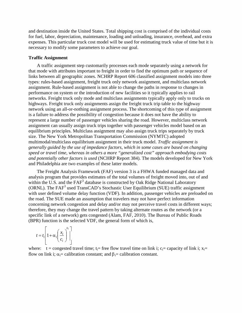
The Freight Analysis Framework (FAF) version 3 is a FHWA funded managed data and analysis program that provides estimates of the total volumes of freight moved into, out of and within the U.S. and the FAF3 database is constructed by Oak Ridge National Laboratory (ORNL). The FAF3 used TransCAD’s Stochastic User Equilibrium (SUE) traffic assignment with user defined volume delay function (VDF). In addition, passenger vehicles are preloaded on the road. The SUE made an assumption that travelers may not have perfect information concerning network congestion and delay and/or may not perceive travel costs in different ways; therefore, they may change the travel pattern by taking alternate routes as the network (or a specific link of a network) gets congested (Alam, FAF, 2010). The Bureau of Public Roads (BPR) function is the selected VDF, the general form of which is,
α+=
βi
i
iii c
xtt 1
where: t = congested travel time; ti= free flow travel time on link i; ci= capacity of link i; xi= flow on link i; αi= calibration constant; and βi= calibration constant.

AVERAGE DRIVING TIME VERSUS RESTING TIME FOR LONG DISTANCE TRUCK DRIVERS
Introduction Hours-of-Service (HOS) rules for truck drivers form another type of public policy, which
has affected the freight system and its costs. In 1938, the first study regarding truck driver HOS rules was issued to ensure highway safety by reducing truck driver fatigue. In 1962, these regulations were modified by eliminating the 24-hour cycle rule and then remained largely the same until 2003. The HOS rules limited commercial vehicle drivers to 10 hours of driving before an 8-hour off duty and to an on-duty period of not more than 15 hours before an 8-hour off duty. In 2003, the changes applied only to property-carrying drivers. These rules allowed 11 hours of driving within a 14-hour period, and required 10 hours of resting. They also put drivers on a natural 24-hour cycle, with a minimum 21-hour cycle (11 hours driving, 10 hours resting).
The truck driver HOS rules are one of the most important factors that affect the cost for transporting the goods by truck to the consumers. And they are very important to the safety of trucking operations – both for the safety of truck drivers themselves and for the safety of others sharing the roads with them. Thus, it is of utmost importance to correctly incorporate these regulations into the microsimulation model so as to obtain the more realistic simulated traffic conditions.
For dynamic traffic assignments in urban areas, truck drivers travel from their origin to their destination in exactly the driving time. Thus, if we want to track a truck, time interval by time interval, then we only need to know how long it takes the driver to travel along each link on the path from the origin to the destination. However, dynamic traffic assignments in rural areas are more complicated because of the HOS rules. A long-distance truck driver usually takes longer to arrive at his destination than the driving time. Trips that take a truck driver more than 11 hours would involve rest periods. A truck can be tracked for 11 hours in the usual way, but then the truck driver stops moving for a period of resting. In order to explain these situations in a dynamic traffic assignment, it is necessary to add the rest periods into the microsimulation model if we want to know the time interval in which a truck reaches a link in eleven or more driving hours from the origin. Thus, HOS rules can affect the routing of a truck as well as the cost of a haul.
The microsimulation was set up to run multiclass and the software QRS II was changed to handle the rest periods. Each class has two parameters (in minutes):
Pause for After each
For example, if a driver needs a minimum of a10-hour resting after driving 11hours, these parameters would be set as:
Pause for = 600 After each = 660
Thus, an 11hour driving time translates to 21 hours of clock time, or a 22 hour driving time translates to 42 hours of clock time.
Therefore, two research questions need to be considered in order to incorporate the truck driver HOS rules into the microsimulation model.
1. What is the average driving time before resting, if a rest is required? 2. What is the average resting time?
It is easily seen that the average driving time is not important unless there is definitely a rest period. In addition, driver’s resting time affects the microsimulation model clock time, not the impedance. Resting time should also be used as a factor in the truck cost model but the current cost model did not use it.
To answer the questions above, this working paper needs to collect the data about average driving time and resting time for long distance truck drivers. Logbooks from truck drivers would be very helpful but there are no related sources available. Data can also be obtained by survey but it is time- and money- consuming. Thus, this paper will concentrate on data reported from the literature.
Literature Review on Average Resting time and Driving Time U.S. DOT, Transport Canada, and Trucking Research Institute (1996) conducted a study to
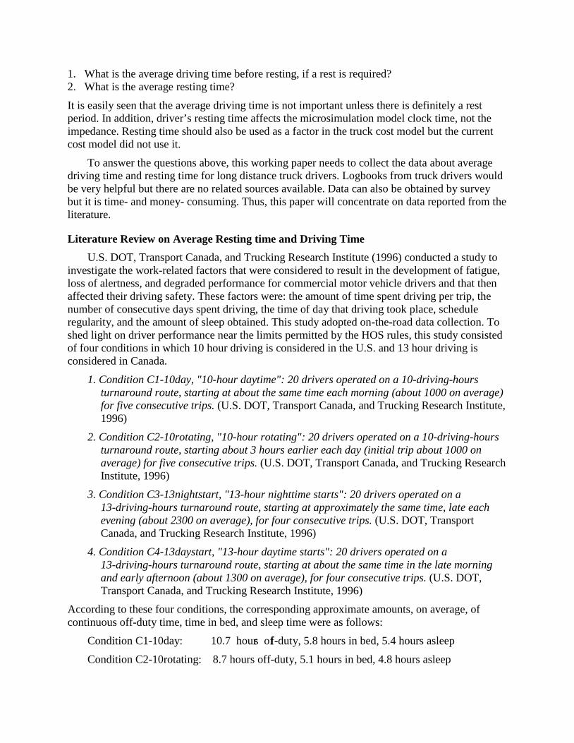
investigate the work-related factors that were considered to result in the development of fatigue, loss of alertness, and degraded performance for commercial motor vehicle drivers and that then affected their driving safety. These factors were: the amount of time spent driving per trip, the number of consecutive days spent driving, the time of day that driving took place, schedule regularity, and the amount of sleep obtained. This study adopted on-the-road data collection. To shed light on driver performance near the limits permitted by the HOS rules, this study consisted of four conditions in which 10 hour driving is considered in the U.S. and 13 hour driving is considered in Canada.
1. Condition C1-10day, "10-hour daytime": 20 drivers operated on a 10-driving-hours turnaround route, starting at about the same time each morning (about 1000 on average) for five consecutive trips. (U.S. DOT, Transport Canada, and Trucking Research Institute, 1996)
2. Condition C2-10rotating, "10-hour rotating": 20 drivers operated on a 10-driving-hours turnaround route, starting about 3 hours earlier each day (initial trip about 1000 on average) for five consecutive trips. (U.S. DOT, Transport Canada, and Trucking Research Institute, 1996)
3. Condition C3-13nightstart, "13-hour nighttime starts": 20 drivers operated on a 13-driving-hours turnaround route, starting at approximately the same time, late each evening (about 2300 on average), for four consecutive trips. (U.S. DOT, Transport Canada, and Trucking Research Institute, 1996)
4. Condition C4-13daystart, "13-hour daytime starts": 20 drivers operated on a 13-driving-hours turnaround route, starting at about the same time in the late morning and early afternoon (about 1300 on average), for four consecutive trips. (U.S. DOT, Transport Canada, and Trucking Research Institute, 1996)
According to these four conditions, the corresponding approximate amounts, on average, of continuous off-duty time, time in bed, and sleep time were as follows:
Condition C1-10day: 10.7 hours off-duty, 5.8 hours in bed, 5.4 hours asleep
Condition C2-10rotating: 8.7 hours off-duty, 5.1 hours in bed, 4.8 hours asleep

Condition C3-13nightstart: 8.6 hours off-duty, 4.4 hours in bed, 3.8 hours asleep
Condition C4-13daystart: 8.9 hours off-duty, 5.5 hours in bed, 5.1 hours asleep
From the results above, it can be concluded that for 10 hours of driving in US, the average off-duty time was 9.7 hours and average time in bed and time asleep was 5.5 hours and 5.1 hours respectively. In addition, the study also pointed out that average reported ideal sleep time for drivers was 7.2 hours but over the course of the study, the average time in bed was 5.2 hours and time asleep was 4.8 hours. This study did give the amount of average off-duty time (average resting time) but it was based on the fixed driving time that is the driving limit (10 hours of driving) within the HOS rules. Furthermore, this study was conducted in1996 before the new 2003 HOS rules. Thus, these results are not realistic.
Mitler, Miller, Lipsitz, Walsh, and Wylie, (1997) conducted the performance monitoring of four groups of 20 truck drivers carrying revenue-producing loads. Four driving schedules were compared: two in the United States (10-hour trips) and two in Canada (13-hour trips), which are similar to four conditions considered by U.S. DOT, Transport Canada, and Trucking Research Institute (1996). The results of this study show that drivers got an average of 5.18 hours in bed per day and 4.78 hours of sleep per day over the five-day study. The authors also presented that a mean (±SD) self-reported ideal amount of sleep was7.1±1 hours a day.
In the previous research, Hanowski, Hickman, Fumero, Olson, and Dingus (2007) found that long- haul commercial vehicle drivers had an average of 5.18 hours in bed per day from Mitler et al. (1997), and that the single long-haul driver got approximately 5.8 hours of sleep per night from Dingus et al. (2002). In their study, the authors analyzed the data collected from 73 truck drivers during a naturalistic driving study after the implementation of the 2003 HOS regulations. From the current study, they found drivers slept more than 6.28 hours on average. By comparison to previously collected data, the mean drivers’ sleep time in the current study showed that drivers may be getting more sleep under the revised HOS regulations. This study provided the amount of average sleep time and time in bed but the MVFC model needs the average resting time (off-duty time) and driving time before resting.
Baas and Charlton (2000) attempted to find out how common driver fatigue is among New Zealand truck drivers and the degree of fatigue-related effects on their driving performance. A total of 600 truck drivers at a variety of sites in the North Island of New Zealand participated for the survey, and this survey was based on interviews and performance tests. As a result, Figure 3 presents the median, inter-quartile range (25th – 75th percentiles), the range of hours of driving for each category. And Table 11 shows the driver activity data. From the figure, it shows that 50% of the logs, stock, and line haul drivers had more than 11 hours of driving in the past 24 hours. From the table, it can be seen that the average number of hours spent driving in the previous 24 hours was about 8.98 hours and the average amount of sleep reported for the past 24 hours was about 7.24 hours. The average length of last rest and sleep was about 12 hours. These values are similar to those desired but they are collected in New Zealand and the MVFC model considers the ten states in the central U.S. In addition, the results are based on the truck drivers in all freight categories rather than only the long-haul truck drivers.

FIGURE 3 Hours of Driving for Each Category (Baas and Charlton, 2000)
Note: Filled circles indicate outliers that are data points further than twice the inter-quartile range from the median.
TABLE 11 Drive Activity Data (Baas and Charlton, 2000)
Mean
(hours) Std.
Deviation Minimum Maximum Driving prior to survey 6.120 3.920 0.00 19.00 Driving in past 24 hrs 8.978 3.993 0.00 23.00 Driving in past 48 hrs 15.895 7.283 0.00 45.00 Length of last duty shift 10.503 3.439 1.00 37.00 Sleeping in past 24hrs 7.241 1.723 0.00 16.00 Sleeping in past 48hrs 14.668 2.947 3.00 27.00 Length of last sleep 7.267 1.782 1.00 17.00 Length of last rest & sleep 12.009 3.619 1.00 32.00 Physical work/exercise past 24 hrs 1.242 2.300 0.00 17.00 Physical work/exercise past 48 hrs 2.702 4.217 0.00 23.00 Desk work in past 24 hrs 0.418 1.576 0.00 15.00 Desk work in past 48 hrs 0.810 2.759 0.00 27.00 Relaxing in past 24 hrs 3.940 2.925 0.00 17.00 Relaxing in past 48 hrs 8.746 5.760 0.00 28.00 Partying in past 24 hrs 0.216 0.937 0.00 8.00 Partying in past 48 hrs 0.555 1.844 0.00 17.00
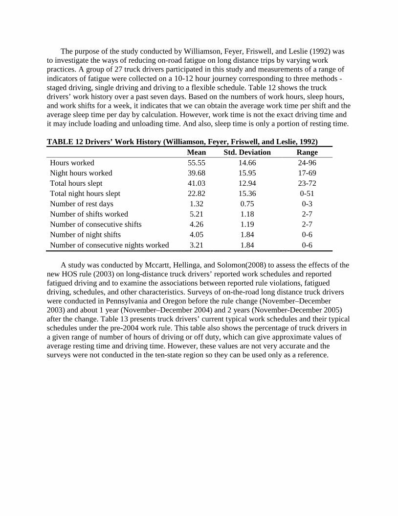
The purpose of the study conducted by Williamson, Feyer, Friswell, and Leslie (1992) was to investigate the ways of reducing on-road fatigue on long distance trips by varying work practices. A group of 27 truck drivers participated in this study and measurements of a range of indicators of fatigue were collected on a 10-12 hour journey corresponding to three methods - staged driving, single driving and driving to a flexible schedule. Table 12 shows the truck drivers’ work history over a past seven days. Based on the numbers of work hours, sleep hours, and work shifts for a week, it indicates that we can obtain the average work time per shift and the average sleep time per day by calculation. However, work time is not the exact driving time and it may include loading and unloading time. And also, sleep time is only a portion of resting time.
TABLE 12 Drivers’ Work History (Williamson, Feyer, Friswell, and Leslie, 1992) Mean Std. Deviation Range Hours worked 55.55 14.66 24-96 Night hours worked 39.68 15.95 17-69 Total hours slept 41.03 12.94 23-72 Total night hours slept 22.82 15.36 0-51 Number of rest days 1.32 0.75 0-3 Number of shifts worked 5.21 1.18 2-7 Number of consecutive shifts 4.26 1.19 2-7 Number of night shifts 4.05 1.84 0-6 Number of consecutive nights worked 3.21 1.84 0-6
A study was conducted by Mccartt, Hellinga, and Solomon(2008) to assess the effects of the
new HOS rule (2003) on long-distance truck drivers’ reported work schedules and reported fatigued driving and to examine the associations between reported rule violations, fatigued driving, schedules, and other characteristics. Surveys of on-the-road long distance truck drivers were conducted in Pennsylvania and Oregon before the rule change (November–December 2003) and about 1 year (November–December 2004) and 2 years (November-December 2005) after the change. Table 13 presents truck drivers’ current typical work schedules and their typical schedules under the pre-2004 work rule. This table also shows the percentage of truck drivers in a given range of number of hours of driving or off duty, which can give approximate values of average resting time and driving time. However, these values are not very accurate and the surveys were not conducted in the ten-state region so they can be used only as a reference.
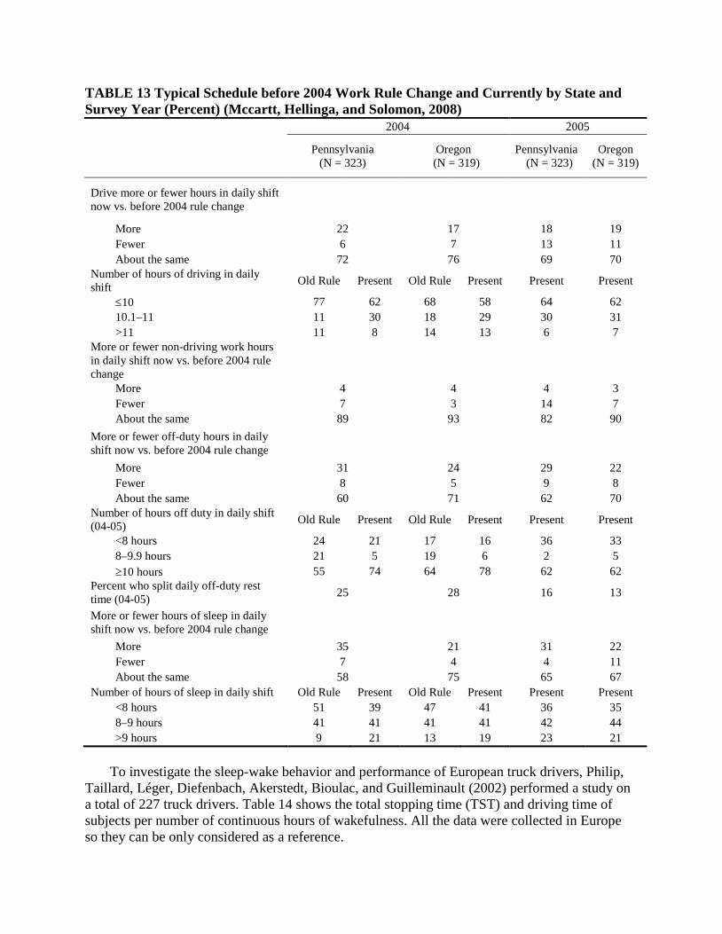
TABLE 13 Typical Schedule before 2004 Work Rule Change and Currently by State and Survey Year (Percent) (Mccartt, Hellinga, and Solomon, 2008) 2004 2005
Pennsylvania (N = 323)
Oregon (N = 319)
Pennsylvania (N = 323)
Oregon (N = 319)
Drive more or fewer hours in daily shift now vs. before 2004 rule change
More 22 17 18 19 Fewer 6 7 13 11 About the same 72 76 69 70 Number of hours of driving in daily shift Old Rule Present Old Rule Present Present Present
≤10 77 62 68 58 64 62 10.1–11 11 30 18 29 30 31 >11 11 8 14 13 6 7 More or fewer non-driving work hours in daily shift now vs. before 2004 rule change
More 4 4 4 3 Fewer 7 3 14 7 About the same 89 93 82 90 More or fewer off-duty hours in daily shift now vs. before 2004 rule change More 31 24 29 22 Fewer 8 5 9 8 About the same 60 71 62 70 Number of hours off duty in daily shift (04-05) Old Rule Present Old Rule Present Present Present
<8 hours 24 21 17 16 36 33 8–9.9 hours 21 5 19 6 2 5 ≥10 hours 55 74 64 78 62 62 Percent who split daily off-duty rest time (04-05) 25 28 16 13
More or fewer hours of sleep in daily shift now vs. before 2004 rule change More 35 21 31 22 Fewer 7 4 4 11 About the same 58 75 65 67 Number of hours of sleep in daily shift Old Rule Present Old Rule Present Present Present <8 hours 51 39 47 41 36 35 8–9 hours 41 41 41 41 42 44 >9 hours 9 21 13 19 23 21
To investigate the sleep-wake behavior and performance of European truck drivers, Philip,
Taillard, Léger, Diefenbach, Akerstedt, Bioulac, and Guilleminault (2002) performed a study on a total of 227 truck drivers. Table 14 shows the total stopping time (TST) and driving time of subjects per number of continuous hours of wakefulness. All the data were collected in Europe so they can be only considered as a reference.

TABLE 14 Total Stopping Time and Driving Times of Subjects per Number of Continuous Hours Awake (Taillard, Léger, Diefenbach, Akerstedt, Bioulac, and Guilleminault, 2002)
No. of Continuous Hours Awake %
TST before Departure (min) Driving (min)
≤14 59.4 449 ± 151 442 ± 151 14.1–15.9 23.5 431 ± 111 540 ± 203 16–17 11.1 459 ± 159 527 ± 173 17.1–20 3.9 458 ± 80 593 ± 186 ≥20.1 2.1 354 ± 109 702 ± 182
FMCSA of US DOT (2005) also pointed out that the average time on duty was 8.78 hours
(including driving) and for the 10 hour driving, the average sleeping time was 5.2 hours.
McCartt, A., Rohrbaugh, J., Hammer, M., and Fuller, S., (2000) also gathered data to identify the factors associated with falling asleep at the wheel. Data was collect through face-to-face interviews with 593 long-distance truck drivers. These truck drivers were randomly selected at public and private rest areas and routine roadside truck safety inspections. The authors described the surveys about the driving hours and off-duty hours but they did not give the specific values from them.
There are some other studies regarding the drivers’ resting time and driving time, such as Mukherjee, Hall, and Shen (2008), Braver, Preusser, Preusser, Baum, Beilock, and Ulmer (1992). Some studies about truck parking were also considered for the related data collection, such as Rodier, Shaheen, Allen, and Dix (2010), Beltemacchi, Rohter, Selinksky, and Manning (2008), PRR and WSDOT (2008), Chen, Pecheux, Farbry, and Fleger (2002), Chatterjee and Wegmann (2000), Garber and Wang (2004).However, there was no related data reported in the studies about the truck drivers’ average resting time and driving time.
Overall, a number of studies regarding truck drivers’ resting time and driving time are reviewed, but there is not a single study that gives the specific numbers of long distance truck drivers’ average resting time and driving time in the Mississippi valley region. Therefore, it is not yet practical to stochastically simulate resting time and driving time, so the current MVFC model used the HOS rule limit (10 hours resting after 11 hours driving) for deterministic average resting time and driving time. As mentioned, resting time can be also used as a factor in the truck cost model but current cost model did not consider it. In the truck cost model, most factors are based on distance so the cost model is largely insensitive to the resting time.
ESTIMATION OF VALUE OF TIME AND PER-MILE COST
Introduction In this chapter, truck costs are computed by using the modified truck cost model, originally
developed by Hussein, and then values of time by commodity by truck class are estimated based on these calculated truck costs.
Truck Cost Analysis As mentioned before, truck value of time is vital for a freight microsimulation model to
convert tolls into equivalent minutes of extra travel time. Although a literature search was

conducted to obtain value of time in the previous section, no studies have specified truck value of time based on different commodities and different truck classes, together. To have an appropriate estimate of value of time by commodity and by truck class, freight transportation costs need to be calculated by a truck cost model. This section will mainly focus on the modification of truck cost model mainly developed by Hussein (2010) and on calculating truck costs for shipping commodity using the new truck cost model.
Description of Truck Cost Model (Hussein, 2010) Hussein’s cost model is in the form of a spreadsheet, and there are two types of inputs:
parameters and constants. Parameters (shown on Table 15) define the service to be provided, such as the commodity (group) that is shipped, how much is shipped, where it is to be shipped, and any additional requests, while constants (shown on Table 16) define the industry environment for providing transportation services including the price of fuel, equipment costs, insurance costs, the current state of technology, and various regulations such as the maximum allowed driving time in a 24-hour period, etc. The total cost per truck for the shipment is the summation of the component costs, which are fuel costs, labor, depreciation, maintenance, loading and unloading, insurance, indirect costs, and extra costs. The detailed information and formulas about the cost model can be found in the document presented by Hussein (2010).
TABLE 15 Parameters in Transportation Cost Model (Hussein, 2010) Parameter Description
Xo Shipment origin (5-digit zip code) Xd Shipment destination (5-digit zip code) Xc Commodity (5-digit SCTG code) or commodity group (2- to 4-digit SCTG
code) Xw Shipment weight (lbs) Xtw Truck weight (lbs) Xtemp Requested cargo temperature (degrees Fahrenheit) Xtime Requested maximum journey time (hrs) Xtrailer Trailer and dock type Xplu Packaging, loading, and unloading method (0 = no unloading service
requested; 1 = unloading service requested)

TABLE 16 Constants in Transportation Cost Model (Hussein, 2010)
Constant Description Estimated values as of April, 2009
CmaxWt Truck capacity (lbs) See Hussein, 2010
CmaxVol Trailer inside volume (ft3) See Hussein, 2010
Cfuel$ Cost of fuel ($/gal) 2. 1
CoptSpd Truck speed that yields optimum fuel efficiency (miles/hr) 55
CmaxEff Truck fuel efficiency while traveling with empty trailer at optimum speed for fuel efficiency (miles/gal) 7-7.5
CminEff Truck fuel efficiency while traveling with full load (by weight) at optimum speed for fuel efficiency (miles/gal) 5-6.0
CspdLim Official truck speed limit on highway (miles/hr) 45-65
Chours Maximum allowed driving time for a single driver in any 24-hour period (hrs) 11
Cref Refrigeration unit fuel consumption per Fahrenheit degree difference between outside temperature and requested cargo temperature per hr (gal/(degree*hr))
0.4
Cperish Commodity’s perishability value (0-1) X†
Cidle Average fuel consumption during idling (gal/hr) 1
Cwage Driver wage ($/mile) 0.4
ChthIns Annual cost of driver health insurance ($) 6000
Cpension Annual cost of driver pension plan ($) 6,500
CSocialMed Annual cost of driver social security tax and Medicare tax ($) 7,650
Cannual Distance an average truck is driven annually (miles) 120,000
Cnew Cost of new tractor + trailer ($) 125,000
Clife Truck expected lifetime (years) 5
Csalv Truck salvage value at end of expected lifetime ($) 25,000
CmaintGM Truck general maintenance cost per mile for engine and non-engine maintenance purposes ($/mile) X††
CmaintT Truck tires maintenance cost per mile ($/mile) X†††
Cunload Average truck unloading cost ($/trailer) 40
CtrkIns Annual cost of full liability, collision, and theft insurance for a truck ($/truck) 5,000
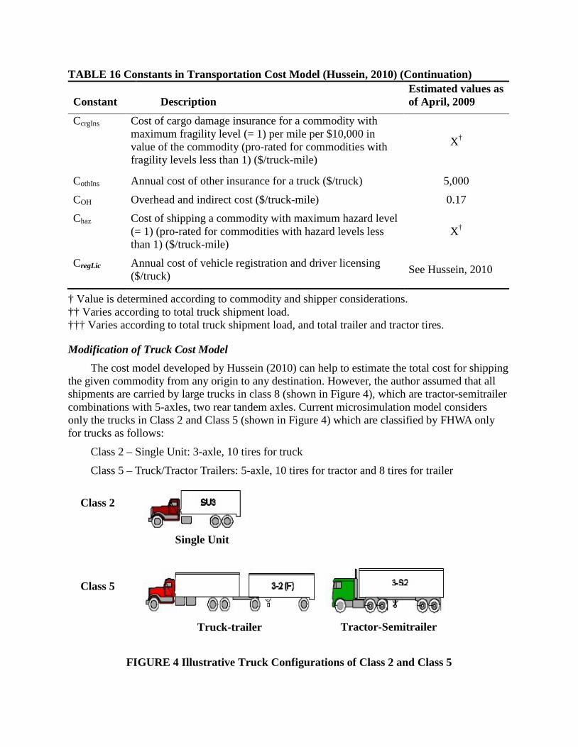
TABLE 16 Constants in Transportation Cost Model (Hussein, 2010) (Continuation)
Constant Description Estimated values as of April, 2009
CcrgIns Cost of cargo damage insurance for a commodity with maximum fragility level (= 1) per mile per $10,000 in value of the commodity (pro-rated for commodities with fragility levels less than 1) ($/truck-mile)
X†
CothIns Annual cost of other insurance for a truck ($/truck) 5,000
COH Overhead and indirect cost ($/truck-mile) 0.17
Chaz Cost of shipping a commodity with maximum hazard level (= 1) (pro-rated for commodities with hazard levels less than 1) ($/truck-mile)
X†
CregLic Annual cost of vehicle registration and driver licensing ($/truck) See Hussein, 2010
† Value is determined according to commodity and shipper considerations. †† Varies according to total truck shipment load. ††† Varies according to total truck shipment load, and total trailer and tractor tires.
Modification of Truck Cost Model The cost model developed by Hussein (2010) can help to estimate the total cost for shipping
the given commodity from any origin to any destination. However, the author assumed that all shipments are carried by large trucks in class 8 (shown in Figure 4), which are tractor-semitrailer combinations with 5-axles, two rear tandem axles. Current microsimulation model considers only the trucks in Class 2 and Class 5 (shown in Figure 4) which are classified by FHWA only for trucks as follows:
Class 2 – Single Unit: 3-axle, 10 tires for truck
Class 5 – Truck/Tractor Trailers: 5-axle, 10 tires for tractor and 8 tires for trailer
FIGURE 4 Illustrative Truck Configurations of Class 2 and Class 5
Class 5
Truck-trailer Tractor-Semitrailer
Class 2
Single Unit

It should be mentioned that Class 8 defined by Hussein (2010) is one type of FHWA truck class 5.
For this situation, a new truck cost model should be developed for these two truck classes. Furthermore, some related parameters, which are different from the original truck model, need to be modified. One parameter is the number of tractor and trailer tires of these two FHWA vehicle classes. Other parameters are the weight of an empty truck and average payload; both of these parameters can be ascertained from tables of FAF2 Technical Documentation provided by FHWA. The empty weights of these two FHWA vehicle classes are shown as follows:
Class 2: 24877 lbs,
Class 5: 29680 lbs
In the microsimulation model undertaken for the MVFC region, five indicative commodities are considered: corn, soybean, dairy, plastics and motor vehicle parts. Table 17 shows the average payload for the two chosen FHWA vehicle classes by those five commodities. Default values in the original truck model are used for most constants (shown on Table 18) but some other values are also changed, such as truck registration fees (highlighted in yellow on Table 18) based on declared gross weight as referred to on Table A3 in the paper of “A Policy-Oriented Cost Model for Shipping Commodities by Truck” (Hussein 2010). It should be noted that Table 18 just shows the constants for motor vehicle parts as an example. In addition, the new truck cost model does not consider loading and unloading costs and rest periods.
TABLE 17 Average Payload for Two FHWA Vehicle Classes by Five Commodities Commodity Class2 Class5
Corn 27,390 49,682
Soybean 24,059 41,891
Dairy 26,038 43,529
Plastics 14,833 38,109
Motor Vehicle Parts 19,996 36,453
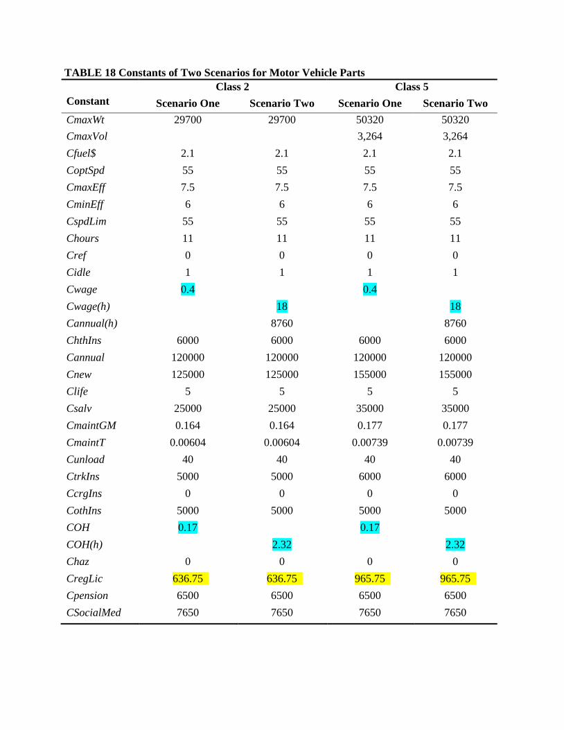
TABLE 18 Constants of Two Scenarios for Motor Vehicle Parts
Constant Class 2 Class 5
Scenario One Scenario Two Scenario One Scenario Two CmaxWt 29700 29700 50320 50320 CmaxVol 3,264 3,264 Cfuel$ 2.1 2.1 2.1 2.1 CoptSpd 55 55 55 55 CmaxEff 7.5 7.5 7.5 7.5 CminEff 6 6 6 6 CspdLim 55 55 55 55 Chours 11 11 11 11 Cref 0 0 0 0 Cidle 1 1 1 1 Cwage 0.4 0.4 Cwage(h) 18 18 Cannual(h) 8760 8760 ChthIns 6000 6000 6000 6000 Cannual 120000 120000 120000 120000 Cnew 125000 125000 155000 155000 Clife 5 5 5 5 Csalv 25000 25000 35000 35000 CmaintGM 0.164 0.164 0.177 0.177 CmaintT 0.00604 0.00604 0.00739 0.00739 Cunload 40 40 40 40 CtrkIns 5000 5000 6000 6000 CcrgIns 0 0 0 0 CothIns 5000 5000 5000 5000 COH 0.17 0.17 COH(h) 2.32 2.32 Chaz 0 0 0 0 CregLic 636.75 636.75 965.75 965.75 Cpension 6500 6500 6500 6500 CSocialMed 7650 7650 7650 7650
In the original cost model, all the costs vary by the distance. However, some of them are sensitive to the time or both time and distance. For example, some truck drivers are paid by the mile but most of them get paid by the hour. Thus, two scenarios for building the new truck cost model should be taken into account for the sake of comparison. One is distance-based and all the features of the original cost model are kept, which is defined as Scenario One. Another is distance- and time-based, which is defined as Scenario Two. The following section will discuss what parameters and formulas need to be changed for each scenario and how to modify them.
As mentioned, whether the wage cost varies by the distance or by the time depends on whether truck drivers get paid by the mile or by the hour. For the model of Scenario One, the average salary of a truck driver in 2009 is $40,000 to $50,000 a year and the average annual driving mileage is 100,000 to 120,000 miles. Based on these figures, the average wage for a driver is roughly $0.40 per mile (highlighted in blue on Table 18). The labor wage cost can be calculated by multiplying this constant ($0.40 per mile) by the total distance (miles) traveled by a trucker. In other words, the longer distance the trucker drives, the more wage costs the trip takes. For the model of Scenario Two, the salary range is considered as the same as the Scenario One and the median value ($45,000 a year) is used as the average salary. The average hourly pay is roughly $18 per hour based on the online search (highlighted in blue on Table 18). Similarly, the labor wage cost equals to the product of dollar per hour times the hours the trucker has traveled.
An individual long-haul trucker pays a truck registration and licensing fee for the right to haul freight on the U.S. roads. For the model of Scenario One, truck registration and licensing cost (RegLic1) based on distance can be given by the following expression.
However, the regular license fee for a given truck class is paid year by year so it is related to travel time, too. The licensing cost (RegLic2) based on time is given by the following expression.
In Scenario One, the average annual distance driven by a truck driver is roughly 120,000 miles and some drivers may exceed it, so Scenario Two is preferred for calculating the licensing costs.
Overhead cost includes all costs which are not classified as direct labor or materials. Some of the items that may be included as indirect costs are management and administration staff, property taxes, utilities, advertising, communication equipment, rental of facilities, and insurance of facilities (Hussein, 2010). For Scenario One, this cost varies across truckers. Dooley, Bertram, and Wilson (1988) found a weighted average of overhead costs per truck as $10,721 annually. After considering inflation, this cost is estimated to be $20,327 per truck in 2009 dollars (Hussein, 2010).The overhead per driven mile is calculated as 20,327 / 120000 = $0.17 per mile (highlighted in blue on Table 18). However, it is very obvious that most of overhead cost vary by the time. For example, rented facilities are paid by month. For Scenario Two, all the overhead costs are therefore assumed to depend on the time. The overhead per hour in Scenario Two is calculated as 20,327 / (365*24) = $2.32 per hour (highlighted in blue on Table 18) and the total
overhead cost is obtained by multiplying this value ($2.32 per hour) by the time traveled by the driver.
Truck Costs Traffic assignment is generally guided by the use of impedance factors, which in many cases
are based on travel time. Impedance can also be taken from a “generalized cost” that embodies a variety of factors. Computing a generalized cost is more complicated but it is also more realistic. Usually, the route of the least cost is chosen by drivers, which is determined by actual travel time, distance, user costs (especially highway tolls) and intangible factors. Formally, the general expression of the costs on a given route is:
Cost = f(real time, distance, toll) = β*(real time) + γ*distance + toll (1) Where,
β: Constant (dollar per hour), also defined as Value of Time γ: Constant (dollar per mile), also defined as Per-mile Cost
It is obvious that tolls are applied only on toll roads and toll bridges, so the value of tolls on non-toll roads and bridges will always be zero.
When the MVFC microsimulation model tries to simulate the freight movements, the truck generalized costs could not be adopted directly as the impedances because the software is only able to identify time as the path building criterion when assigning the traffic. For this reason, it is necessary to convert the truck costs in units of dollars to units of time, specifically minutes. The formula above can be therefore expressed in another way:
Impedance = 1 * (real time) + (γ/β) * distance + 1 * (toll/β) = 1 * (real time) + (γ/β) * distance + 1 * (extra time) (2)
From the expression (2), it can be seen that two constants (β and γ) determine the conversion from the costs to the time. In order to find reasonable values for these two constants, trucks costs should be calculated from the new truck cost model, which has parameters modified from the original cost model to meet the requirements of the MVFC model.
In the real world, it is easily noted that when a driver travels between two locations, it takes him or her different distances or times depending upon the routes or times of day. Here, two situations are considered. For situation one (shown in Figure 5), suppose that there are two routes with different lengths from location A to location B: one is 100 miles and another is 80 miles. Due to different speeds, the driver may spend the same amount of time (2 hours) on these two different routes. For situation two (shown in Figure 6), suppose that there are two routes with the same length (80 miles) and the driver travels on each route but at different times of day. When the driver takes his trip on the road while congested, it takes him 3 hours to finish his trip. However, when the driver takes his trip on the road while uncongested, it takes him only 1.5 hours to finish his trip.
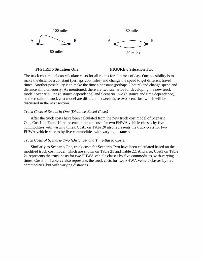
FIGURE 5 Situation One FIGURE 6 Situation Two
The truck cost model can calculate costs for all routes for all times of day. One possibility is to make the distance a constant (perhaps 200 miles) and change the speed to get different travel times. Another possibility is to make the time a constant (perhaps 2 hours) and change speed and distance simultaneously. As mentioned, there are two scenarios for developing the new truck model: Scenario One (distance dependence) and Scenario Two (distance and time dependence), so the results of truck cost model are different between these two scenarios, which will be discussed in the next section.
Truck Costs of Scenario One (Distance-Based Costs) After the truck costs have been calculated from the new truck cost model of Scenario
One, Cost1 on Table 19 represents the truck costs for two FHWA vehicle classes by five commodities with varying times. Cost1 on Table 20 also represents the truck costs for two FHWA vehicle classes by five commodities with varying distances.
Truck Costs of Scenario Two (Distance- and Time-Based Costs) Similarly as Scenario One, truck costs for Scenario Two have been calculated based on the
modified truck cost model, which are shown on Table 21 and Table 22. And also, Cost3 on Table 21 represents the truck costs for two FHWA vehicle classes by five commodities, with varying times. Cost3 on Table 22 also represents the truck costs for two FHWA vehicle classes by five commodities, but with varying distances.
A B
80 miles
80 miles
A B
100 miles
80 miles

TABLE 19 Truck Costs by Different Times with Constant Distance (200 miles) – Scenario One
Commodity Speed
(mile/h) Distance
(mile) Time (h)
Class 2 Class 5 Cost1
($) Cost2
($) Cost1
($) Cost2
($)
Corn
20 200 10.00 436.88 440.00 531.36 531.60 30 200 6.67 422.57 417.33 508.94 484.40 40 200 5.00 405.71 406.00 481.15 460.80 50 200 4.00 394.41 399.20 458.27 446.64 60 200 3.33 389.66 394.67 440.40 437.20
64.33 200 3.11 390.78 393.14 436.71 434.02 70 200 2.86 396.41 391.43 438.86 430.46
Soybean
20 200 10.00 427.70 431.00 509.91 510.40 30 200 6.67 414.39 411.33 489.82 470.27 40 200 5.00 398.88 401.50 465.18 450.20 50 200 4.00 389.00 395.60 445.63 438.16 60 200 3.33 385.86 391.67 431.53 430.13
64.33 200 3.11 387.57 390.34 429.22 427.43 70 200 2.86 393.63 388.86 432.37 424.40
Dairy
20 200 10.00 492.37 492.80 617.31 617.70 30 200 6.67 458.08 458.53 562.44 541.80 40 200 5.00 440.93 441.40 519.98 503.85 50 200 4.00 430.64 431.12 489.44 481.08 60 200 3.33 423.78 424.27 467.69 465.90
64.33 200 3.11 421.47 421.96 462.78 460.79 70 200 2.86 418.88 419.37 463.13 455.06
Plastics
20 200 10.00 401.90 405.90 499.50 500.10 30 200 6.67 391.35 394.60 480.54 463.40 40 200 5.00 379.56 388.95 457.42 445.05 50 200 4.00 373.62 385.56 439.49 434.04 60 200 3.33 374.95 383.30 427.22 426.70
64.33 200 3.11 378.31 382.54 425.59 424.23 70 200 2.86 385.55 381.69 429.22 421.46
Motor Vehicle Parts
20 200 10.00 416.33 419.90 494.94 496.60 30 200 6.67 404.23 403.93 476.48 461.40 40 200 5.00 390.36 395.95 454.03 443.80 50 200 4.00 382.22 391.16 436.80 433.24 60 200 3.33 381.05 387.97 425.34 426.20
64.33 200 3.11 383.49 386.89 424.00 423.83 70 200 2.86 390.06 385.69 427.84 421.17

TABLE 20 Truck Costs by Different Distances with Constant Time (2 hours) – Scenario One
Commodity Speed
(mile/h) Distance
(mile) Time (h)
Class 2 Class 5 Cost1
($) Cost2
($) Cost1
($) Cost2
($)
Corn
20 40 2.00 87.38 88.00 106.27 106.32 30 60 2.00 126.77 125.20 152.68 145.32 40 80 2.00 162.29 162.40 192.46 184.32 50 100 2.00 197.21 199.60 229.14 223.32 60 120 2.00 233.80 236.80 264.24 262.32
64.33 128.66 2.00 251.39 252.91 280.94 279.21 70 140 2.00 277.49 274.00 307.20 301.32
Soybean
20 40 2.00 85.54 86.20 101.98 102.08 30 60 2.00 124.32 123.40 146.95 141.08 40 80 2.00 159.55 160.60 186.07 180.08 50 100 2.00 194.50 197.80 222.81 219.08 60 120 2.00 231.51 235.00 258.92 258.08
64.33 128.66 2.00 249.33 251.11 276.12 274.97 70 140 2.00 275.54 272.20 302.66 297.08
Dairy
20 40 2.00 98.47 98.56 123.46 123.54 30 60 2.00 137.42 137.56 168.73 162.54 40 80 2.00 176.37 176.56 207.99 201.54 50 100 2.00 215.32 215.56 244.72 240.54 60 120 2.00 254.27 254.56 280.61 279.54
64.33 128.66 2.00 271.13 271.45 297.71 296.43 70 140 2.00 293.22 293.56 324.19 318.54
Plastics
20 40 2.00 80.38 81.18 99.90 100.02 30 60 2.00 117.40 118.38 144.16 139.02 40 80 2.00 151.82 155.58 182.97 178.02 50 100 2.00 186.81 192.78 219.75 217.02 60 120 2.00 224.97 229.98 256.33 256.02
64.33 128.66 2.00 243.36 246.09 273.78 272.91 70 140 2.00 269.88 267.18 300.45 295.02
Motor Vehicle
Parts
20 40 2.00 83.27 83.98 98.99 99.32 30 60 2.00 121.27 121.18 142.94 138.42 40 80 2.00 156.15 158.38 181.61 177.52 50 100 2.00 191.11 195.58 218.40 216.62 60 120 2.00 228.63 232.78 255.20 255.72
64.33 128.66 2.00 246.70 248.89 272.76 272.65 70 140 2.00 273.04 269.98 299.49 294.82

TABLE 21 Truck Costs by Different Time with Constant Distance (200 miles) – Scenario Two
Commodity Speed
(mile/h) Distance
(mile) Time (h)
Class 2 Class 5
Cost3 ($)
Cost4 ($)
Cost3 ($)
Cost4 ($)
Corn
20 200 10.00 504.03 507.00 598.39 598.90 30 200 6.67 414.04 408.67 500.21 475.93 40 200 5.00 359.34 359.50 434.53 414.45 50 200 4.00 325.33 330.00 388.92 377.56 60 200 3.33 305.44 310.33 355.89 352.97
64.33 200 3.11 301.47 303.71 347.10 344.69 70 200 2.86 301.38 296.29 343.53 335.40
Soybean
20 200 10.00 494.85 498.00 576.94 577.70 30 200 6.67 405.85 402.67 481.09 461.80 40 200 5.00 352.50 355.00 418.56 403.85 50 200 4.00 319.92 326.40 376.28 369.08 60 200 3.33 301.64 307.33 347.02 345.90
64.33 200 3.11 298.26 300.92 339.62 338.10 70 200 2.86 298.60 293.71 337.04 329.34
Dairy
20 200 10.00 670.40 673.40 751.54 752.20 30 200 6.67 524.11 519.60 598.50 578.13 40 200 5.00 441.61 442.70 506.96 491.10 50 200 4.00 391.17 396.56 446.97 438.88 60 200 3.33 360.60 365.80 405.58 404.07
64.33 200 3.11 353.05 355.45 394.07 392.35 70 200 2.86 348.85 343.83 387.00 379.20
Plastics
20 200 10.00 469.17 472.60 566.53 567.40 30 200 6.67 383.02 385.73 471.81 454.93 40 200 5.00 333.43 342.30 410.80 398.70 50 200 4.00 304.82 316.24 370.14 364.96 60 200 3.33 291.02 298.87 342.71 342.47
64.33 200 3.11 289.29 293.02 335.98 334.90 70 200 2.86 290.82 286.46 333.89 326.40
Motor
Vehicle
Parts
20 200 10.00 416.33 419.90 112.39 112.58 30 200 6.67 404.23 403.93 140.32 135.58 40 200 5.00 390.36 395.95 162.96 158.58 50 200 4.00 382.22 391.16 183.73 181.58 60 200 3.33 381.05 387.97 204.50 204.58
64.33 200 3.11 383.49 386.89 215.11 214.54 70 200 2.86 390.06 385.69 232.76 227.58
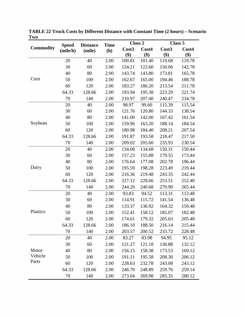
TABLE 22 Truck Costs by Different Distance with Constant Time (2 hours) – Scenario Two
Commodity Speed (mile/h)
Distance (mile)
Time (h)
Class 2 Class 5 Cost3
($) Cost4
($) Cost3
($) Cost4
($)
Corn
20 40 2.00 100.81 101.40 119.68 119.78 30 60 2.00 124.21 122.60 150.06 142.78 40 80 2.00 143.74 143.80 173.81 165.78 50 100 2.00 162.67 165.00 194.46 188.78 60 120 2.00 183.27 186.20 213.54 211.78
64.33 128.66 2.00 193.94 195.38 223.29 221.74 70 140 2.00 210.97 207.40 240.47 234.78
Soybean
20 40 2.00 98.97 99.60 115.39 115.54 30 60 2.00 121.76 120.80 144.33 138.54 40 80 2.00 141.00 142.00 167.42 161.54 50 100 2.00 159.96 163.20 188.14 184.54 60 120 2.00 180.98 184.40 208.21 207.54
64.33 128.66 2.00 191.87 193.58 218.47 217.50 70 140 2.00 209.02 205.60 235.93 230.54
Dairy
20 40 2.00 134.08 134.68 150.31 150.44 30 60 2.00 157.23 155.88 179.55 173.44 40 80 2.00 176.64 177.08 202.78 196.44 50 100 2.00 195.59 198.28 223.49 219.44 60 120 2.00 216.36 219.48 243.35 242.44
64.33 128.66 2.00 227.12 228.66 253.51 252.40 70 140 2.00 244.20 240.68 270.90 265.44
Plastics
20 40 2.00 93.83 94.52 113.31 113.48 30 60 2.00 114.91 115.72 141.54 136.48 40 80 2.00 133.37 136.92 164.32 159.48 50 100 2.00 152.41 158.12 185.07 182.48 60 120 2.00 174.61 179.32 205.63 205.48
64.33 128.66 2.00 186.10 188.50 216.14 215.44 70 140 2.00 203.57 200.52 233.72 228.48
Motor Vehicle Parts
20 40 2.00 83.27 83.98 94.95 95.12 30 60 2.00 121.27 121.18 136.88 132.12 40 80 2.00 156.15 158.38 173.53 169.12 50 100 2.00 191.11 195.58 208.30 206.12 60 120 2.00 228.63 232.78 243.08 243.12
64.33 128.66 2.00 246.70 248.89 259.76 259.14 70 140 2.00 273.04 269.98 285.35 280.12

Value of Time and Per-mile Cost This section will show how to calculate the two impedance parameters based on the truck
costs of Scenario One and Scenario Two.
Value of Time and Per-mile Cost for Scenario One (Distance-Based Costs) Based on the results of Cost1 on Table 19 and Table 20, linear regressions are performed to
ascertain the relationship of cost and time and of cost and distance for five commodities and two truck classes. Figure 7 through Figure 10 take the commodity motor vehicle parts as an example to present these relationships and the figures about these relationships for all five commodities are presented in Appendix B.
FIGURE 7 Linear Relationship of Cost/Time (Motor Vehicle Parts, Class 2, Scenario One)
y = 4.7923x + 357.51R² = 0.882
365
370
375
380
385
390
395
400
405
410
0.00 2.00 4.00 6.00 8.00 10.00 12.00
Cost
($)
Traveling Time (h)

FIGURE 8 Linear Relationship of Cost/Distance (Motor Vehicle Parts, Class 2, Scenario
One)
FIGURE 9 Linear Relationship of Cost/Time (Motor Vehicle Parts, Class 5, Scenario One)
y = 1.8616x + 7.9178R² = 0.9986
0
50
100
150
200
250
300
0 50 100 150
Cost
($)
Distance (mile)
y = 10.566x + 395.71R² = 0.9496
420
430
440
450
460
470
480
490
500
510
0.00 2.00 4.00 6.00 8.00 10.00 12.00
Cost
($)
Traveling Time (h)

FIGURE 10 Linear Relationship of Cost/Distance (Motor Vehicle Parts, Class 5, Scenario
One)
The slopes of the lines in the figures lead to the value of time (β) and per-mile cost (γ). All the values of β and γ by commodity by truck class for Scenario One are shown on Table 23.
TABLE 23 Values of β and γ for Five Commodities and Two Truck Classes– Scenario One (Distance-Based Costs)
Commodity
Class 2 Class 5
β ($/h) γ ($/mile) β ($/h) γ ($/mile)
Corn 6.8 1.86 14.16 1.95
Soybean 5.9 1.86 12.04 1.95
Dairy 10.28 1.94 22.77 1.95
Plastics 3.39 1.86 11.01 1.95
Motor Vehicle Parts 4.79 1.86 10.56 1.96
By comparing Cost1 with Cost2, it is seen that both give similar results, which means that either cost and time or cost and distance are almost linearly related. The analysis also reveals that the constants (β and γ) obtained from the linear regressions are plausible. Table 23 shows that dairy has the highest truck value of time (β) regardless of the truck class, and plastics has the lowest truck value of time for class 2 but motor vehicle parts have the lowest value of time for class 5. These results are reasonable because: (1). the average payload of dairy is the second heaviest but dairy needs low temperatures to keep fresh and refrigeration causes additional consumption of fuel, which indirectly increases the total truck costs; (2). when loaded in the same truck class 2, plastics has the smallest amount of average payload; and (3). the same payload reason explains why motor vehicle parts have the lowest value of time for class 5. Truck values of time for the
y = 1.9551x + 23.156R² = 0.999
0
50
100
150
200
250
300
350
0 50 100 150
Cost
($)
Distance (mile)
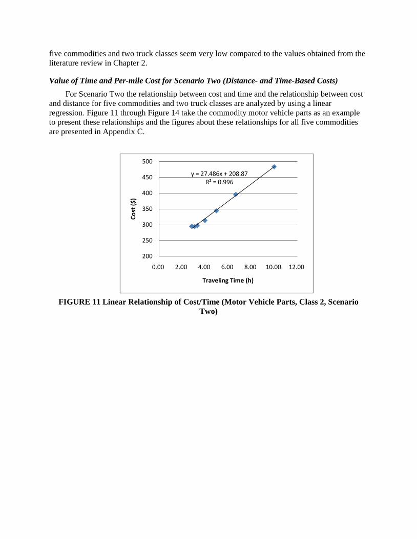
five commodities and two truck classes seem very low compared to the values obtained from the literature review in Chapter 2.
Value of Time and Per-mile Cost for Scenario Two (Distance- and Time-Based Costs) For Scenario Two the relationship between cost and time and the relationship between cost
and distance for five commodities and two truck classes are analyzed by using a linear regression. Figure 11 through Figure 14 take the commodity motor vehicle parts as an example to present these relationships and the figures about these relationships for all five commodities are presented in Appendix C.
FIGURE 11 Linear Relationship of Cost/Time (Motor Vehicle Parts, Class 2, Scenario
Two)
y = 27.486x + 208.87R² = 0.996
200
250
300
350
400
450
500
0.00 2.00 4.00 6.00 8.00 10.00 12.00
Cost
($)
Traveling Time (h)

FIGURE 12 Linear Relationship of Cost/Distance (Motor Vehicle Parts, Class 2, Scenario
Two)
FIGURE 13 Linear Relationship of Cost/Time (Motor Vehicle Parts, Class 5, Scenario
Two)
y = 1.0629x + 53.302R² = 0.9957
0
50
100
150
200
250
0 50 100 150
Cost
($)
Distance (mile)
y = 33.297x + 235.43R² = 0.9947
200
250
300
350
400
450
500
550
600
0.00 2.00 4.00 6.00 8.00 10.00 12.00
Cost
($)
Traveling Time (h)

FIGURE 14 Linear Relationship of Cost/Distance (Motor Vehicle Parts, Class 5, Scenario
Two
As before, all the values of β and γ by commodity by truck class for Scenario Two are shown on Table 24.
TABLE 24 Values of β and γ for Five Commodities and Two Truck Classes– Scenario Two
Commodity Class 2 Class 5
β ($/h) γ ($/mile) β ($/h) γ ($/mile)
Corn 29.5 1.06 36.89 1.15
Soybean 28.6 1.06 34.77 1.15
Dairy 46.14 1.06 52.22 1.15
Plastics 26.06 1.06 33.74 1.15
Motor Vehicle Parts 27.48 1.06 33.29 1.15
Again these constants (β and γ) obtained from the linear regression graphics are plausible. Compared to the values of β and γ from Table 23, β values on Table 24 are higher and γ values lower, which are more reasonable considering the literature review.
Conclusion The purpose of this chapter is to estimate the value of time and per-mile cost for different
commodities and for different truck classes in the Mississippi Valley region that will be used to convert the units of components of impedances to the units of time.
The results showed that either cost and time, or cost and distance for Scenario One (distance-based) and Scenario Two (distance- and time-based) are almost linearly related. From
y = 1.1538x + 68.614R² = 0.997
0
50
100
150
200
250
0 50 100 150
Cost
($)
Distance (mile)

the results, we can see that the values of time by different commodities in Scenario One range from $3.39 to $20.28 for class 2 and from $10.56 to $22.77 for class 5. And also, the values of time by different commodities in Scenario Two range from $26.06 to $46.14 for class 2 and from $33.29 to $52.22 for class 5. Values of time by commodity by truck class in Scenario Two are higher than those in Scenario One, but the values of per-mile cost by commodity by truck class in Scenario Two are a little lower than those in Scenario One. Finally, the estimated values of time in Scenario Two are most similar to the estimates in the literature. However, the values of time in Scenario One are still retained for testing the simulations to follow.
ANALYSIS OF KEY FACTORS FOR MICROSIMULATION MODEL
Introduction In this chapter, the collected tolls for all toll facilities in the MVFC region are converted to
extra travel time by using values of time (β), and distance weights (γ/β) are estimated for converting units of distance to units of time. Furthermore, intersection delays are handled by adding extra time to each direction of each surface street.
Extra Travel Time (Toll)
Toll Analysis The MVFC microsimulation model is proposed to address some public policies affecting the
freight system in the Central U.S. and toll pricing policy is one of these important policies. As mentioned before, tolls greatly affect the route choice of truck drivers. Truckers could divert alternative routes to avoid tolls. Hence, tolls become an important input for a traffic assignment step.
Toll Roads and Toll Bridges in MVFC Region The ten states in the Mississippi Valley region are Illinois, Indiana, Iowa, Kansas, Kentucky,
Michigan, Minnesota, Missouri, Ohio and Wisconsin. The locations of all toll roads and toll bridges in these ten states are presented in Figure 15.

FIGURE 15 Toll Roads and Toll Bridges for Ten States in the Mississippi Valley Region
Table 25 and Table 26 contain detailed information about toll roads and toll bridges in the MVFC states, such as length, location, financial or operating authority.

TABLE 25 Detailed Information about Toll Roads
State Toll Road Financing or Operating Authority From To
Length (Mile)
Illinois Ronald Reagan Memorial IL State Toll Highway Authority US 30 Rock Falls (W. terminus) MP 44.2 I-290 (E. terminus) MP 140.25 96
Illinois Veterans Memorial IL State Toll Highway Authority I-80 Army Trail Road 30
Illinois Janne Addams Memorial IL State Toll Highway Authority East Rockton Road (W. terminus) MP 76 River Road (E. terminus) MP 0 77
Illinois Tri-State IL State Toll Highway Authority US-41 Skokie Highway (N. terminus) SR 394 (S. terminus) 77.7
Illinois Chicago Skyway Cintras Corporation I-94 in Chicago Indiana Stateline 7.7
Indiana Indiana East-West IN Dept of Trans Illinois Line Porter County Line-Gary 157
Kansas Kansas Turnpike KS Turnpike Authority Oklahoma State Line 18th Street, Kansas City 236
Ohio Ohio Turnpike OH Turnpike Commission Pennsylvania Line Youngstown 236.4
TABLE 26 Detailed Information about Toll Bridges
State Name of Facility Financing or Operating Authority From To Length (Mile)
Illinois - Indiana New Harmony Bridge White County Bridge Commission White Cnty, IL (0.3 Mi) New Harmony, IN (0.2 Mi) 0.5
Illinois - Indiana Wabash Memorial Bridge Indiana Department of Transportation New Haven, IL Mt. Vernon, IN 0.9
Illinois - Iowa Fort Madison Bridge A.T. & SF. Rdway Co; Topeka, KS Niota, IL Ft. Madison, IA 0.6
Michigan - Ontario Ambassador Bridge Detroit InternatlBrdgAuth Detroit, MI (0.9 Mi) Windsor, ON (0.8 Mi) 1.7
Michigan - Ontario Detroit-Windsor Tunnel Detroit & Canada Tunnel Corp; Detroit, MI Detroit, MI (0.5 Mi) Windsor, ON (0.47 Mi) 0.97
Michigan Mackinac Bridge Mackinac BrdgAuth of Michigan Mackinac Straits St. Ignace, MI 4.4
Michigan - Ontario International Bridge InternatlBrdgAuth of MI St. Mary's River Sault Marie, ON (1.1 Mi) 1.95
Michigan - Ontario Blue Water Bridge MI Dept of Trans St. Clair River Pte Edward, ON (0.8 Mi) 1.5
Nebraska - Iowa Bellevue Bridge City of Bellevue, NE Brdg Com SR 370, IA (0.18 Mi) Bellevue, NE (0.18 Mi) 0.18
Nebraska - Iowa Burt County Bridge Burt Cnty, NE Brdg Com Onawa, IA (0.35 Mi) Decatur, NE (0.35 Mi) 0.7
Nebraska - Iowa Plattsmouth Bridge Plattsmouth, NE Brdg Mills Cnty, IA (0.13 Mi) Plattsmouth, NE (0.13 Mi) 0.26
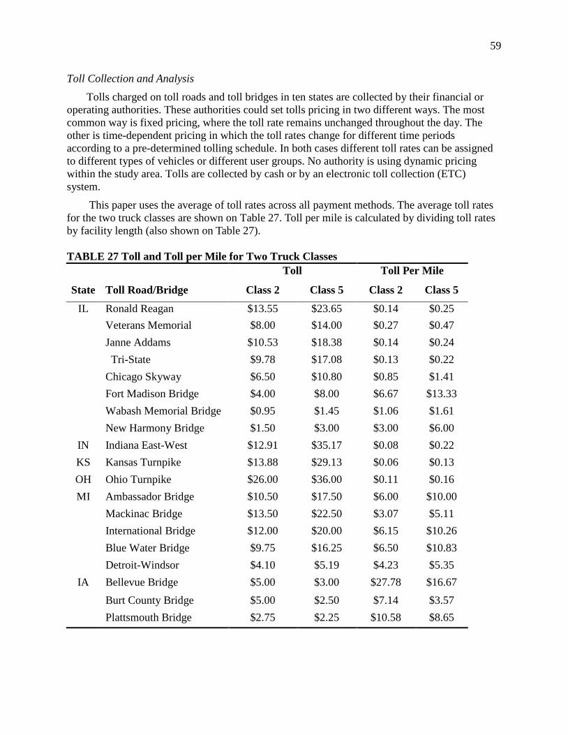
59
Toll Collection and Analysis Tolls charged on toll roads and toll bridges in ten states are collected by their financial or
operating authorities. These authorities could set tolls pricing in two different ways. The most common way is fixed pricing, where the toll rate remains unchanged throughout the day. The other is time-dependent pricing in which the toll rates change for different time periods according to a pre-determined tolling schedule. In both cases different toll rates can be assigned to different types of vehicles or different user groups. No authority is using dynamic pricing within the study area. Tolls are collected by cash or by an electronic toll collection (ETC) system.
This paper uses the average of toll rates across all payment methods. The average toll rates for the two truck classes are shown on Table 27. Toll per mile is calculated by dividing toll rates by facility length (also shown on Table 27).
TABLE 27 Toll and Toll per Mile for Two Truck Classes
State Toll Road/Bridge
Toll Toll Per Mile
Class 2 Class 5 Class 2 Class 5
IL Ronald Reagan $13.55 $23.65 $0.14 $0.25 Veterans Memorial $8.00 $14.00 $0.27 $0.47 Janne Addams $10.53 $18.38 $0.14 $0.24 Tri-State $9.78 $17.08 $0.13 $0.22 Chicago Skyway $6.50 $10.80 $0.85 $1.41 Fort Madison Bridge $4.00 $8.00 $6.67 $13.33 Wabash Memorial Bridge $0.95 $1.45 $1.06 $1.61 New Harmony Bridge $1.50 $3.00 $3.00 $6.00
IN Indiana East-West $12.91 $35.17 $0.08 $0.22 KS Kansas Turnpike $13.88 $29.13 $0.06 $0.13 OH Ohio Turnpike $26.00 $36.00 $0.11 $0.16 MI Ambassador Bridge $10.50 $17.50 $6.00 $10.00
Mackinac Bridge $13.50 $22.50 $3.07 $5.11 International Bridge $12.00 $20.00 $6.15 $10.26 Blue Water Bridge $9.75 $16.25 $6.50 $10.83 Detroit-Windsor $4.10 $5.19 $4.23 $5.35
IA Bellevue Bridge $5.00 $3.00 $27.78 $16.67 Burt County Bridge $5.00 $2.50 $7.14 $3.57 Plattsmouth Bridge $2.75 $2.25 $10.58 $8.65

60
The General Network Editor (GNE) is a graphical, data base manager for computer-aided design of transportation networks. Its principal use is for entering network data into the computer: drawing a network on the computer screen; entering numerical data; editing of strings and numbers; calculating attribute values from other pieces of data; and finding network elements that meet certain criteria (Horowitz, 1987). In the GNE software, roads and bridges are presented as one or more links. In particular, all roads are separated into different links, especially across the other roads. The model in this paper uses the ORNL network containing all major highways in the U.S. and these highways are represented as 112,000 links. However, this model only retains all the details for the ten MVFC states and 100 miles extension of these states, while it reduces the network outside the defined area to interstate highway, only. The reduced network has approximately 44,000 links with many attributes retained from the original ORNL network. Figure 16 shows a portion of road network in GNE. Thus, it is necessary to obtain the toll on each toll road/toll bridge link as one of the link impedance factors. Appendix A shows the toll on each Toll road/ bridge link in the study area.
FIGURE 16 A Portion of Road Network in GNE
Extra Travel Time (Toll) There are many public policies affecting the freight transportation system. Some truck
drivers are willing to pay tolls to save time but others are not and they will divert to an alternate road to avoid toll pricing. This paper mainly focuses on assessing the extent of the impact of the toll pricing policy on routing decisions. Generally, there is no doubt that tolls are paid by money. However, the microsimulation model could not directly use the toll cost as one of the impedances so tolls need to be expressed as “extra times” on the network. The values of time (dollar per hour) by commodity by truck class have been obtained in the previous chapter to convert tolls (in dollars) to extra times (in minutes) by using the equation (3).

61
Extra Times = Tolls / β * 60 (3) Where,
β: Truck value of time (dollar per hour)
Note: 60 is used to convert hours to minutes.
Both directions on the same link are assumed to have the same amount of extra time. The following shows a portion of the text file about the extra times on each toll road/ bridge link for motor vehicle parts in Scenario Two, in which A represents class 5 and B represents class 2.
L27784
L27785
L27952
L27953
L27954
L27955
L27956
L27957
END OF ROWS
A==>B A
B==>AA
END OF COLUMNS
4.28 4.28
9.80 9.80
1.59 1.59
1.85 1.85
6.76 6.76
1.15 1.15
5.65 5.65
1.10 1.10
L27784
L27785
L27952
L27953
L27954
L27955

62
L27956
L27957
END OF ROWS
A==>B B
B==>A B
END OF COLUMNS
2.97 2.97
6.79 6.79
1.10 1.10
1.28 1.28
4.68 4.68
0.79 0.79
3.91 3.91
0.76 0.76
END OF TABLES
Distance Weight (γ/β) Based on the equation (2): Impedance = 1 * (real time) + (γ/β) * distance + 1 * (extra time),
we can see that the units of distance impedance also need to be converted into the units of time. The distance weight (γ/β) is used to accomplish this conversion and it varies by commodity or truck class. Table 28 shows the values of γ/β by commodity by truck class for both Scenarios.
TABLE 28 Values of Distance Weight (γ/β) by Commodity by Truck Class for Two Scenarios
Commodity
γ/β (min/mile)(Scenario One) γ/β (min/mile)(Scenario Two)
Class 2 Class 5 Class 2 Class 5
Corn 16.41 8.26 2.16 1.87
Soybean 18.92 9.72 2.22 1.98
Dairy 11.32 5.14 1.38 1.32
Plastics 32.92 10.63 2.44 2.05
Motor Vehicle Parts 23.30 11.14 2.31 2.07
From the table, it can be clearly seen that the values of distance weight (γ/β) for Scenario One are much bigger than Scenario Two. The values for Scenario Two are more reasonable given that

63
vehicles are traveling on the highways at a speed of 50 to 65 miles per hour and on the local roads at the speed of 20 to 45 miles per hour.
Intersection Delays
Results from Initial Test An initial test run was performed by using the parameters of Scenario Two. Figure 17 shows
a portion of initial test results in southern Michigan area. It should note that link is proportional to the volume.
FIGURE 17 A Portion of Initial Test Results without Intersection Delay in Southern Michigan Area
From the figure, it indicates that the Telegraph road has a portion of truck traffic in this corridor, the amount of which is bigger than expected. The Telegraph road is two-lane road and it has control delay at its intersections. Route I-75 that is parallel to and close to the Telegraph road has a higher speed and no intersection delay. So there is no doubt that the truckers would want to travel on the Route I-75 rather than the Telegraph road. It is therefore concluded that the initial test results were not realistic. The reason for this problem is that the simulation model did not consider the intersection delays for the surface streets.
Solution for Intersection Delays There are two simple methods to deal with intersection delays for the surface streets: (1)
increase the travel times on all non-freeway links or (2) add penalties at all at-grade intersections. Neither is a perfect solution, because not all intersections are present in the network and
Telegraph Rd.
I-75

64
intersection density varies considerably from link to link. To correct for the imbalance between Telegraph Rd. and I-75 in southern Michigan, 0.5 minutes of extra time were added to each direction of each surface street to account (roughly) for control delay at the ends of those links. Another test run was made after adding those 0.5 minutes of extra times to surface links. Figure 18 shows a portion of test results with intersection delay in southern Michigan area.
FIGURE 18 A Portion of Initial Test Results with Intersection Delay in Southern Michigan Area
From the figure above, it can be seen that a much smaller portion of the truck traffic is on
the Telegraph road compared to the results shown in Figure 17 so the results of the second initial test run are more reasonable.
ACTUAL TRUCK TRAFFIC DATA COLLECTION Generally, actual traffic counts are from traffic monitoring sties, and data includes vehicle
volume, vehicle classification, and weight-in-motion. Data is usually collected using manual, portable (road tube), and permanent automatic traffic recorders (ATR) methods.
The Ohio Department of Transportation has provided truck traffic counts collected by several methods including traffic data collected from ATR stations and weigh stations, coverage counts and manual counts. However, based on the pros and cons of traffic data collecting methods, the ATR station data will be used for the analysis since they are more accurate and reliable than the others. The traffic counts from ATR stations in Ohio are grouped into cars and trucks but only two classes of trucks are taken into account in the traffic assignment model. It is impossible to find the reliable traffic data for precisely these two truck classes. However, these two classes are the major types of trucks traveling in Ohio, so it can be reasonably assumed that the two truck classes are in proportion to total trucks.
65
Route I-80 has no ATR stations along the vast majority of its length, where it is also called the Ohio Turnpike. Fortunately, Turnpike Authority, the operator of Ohio Turnpike, does its own counts.
However, it is worth noting that the Turnpike truck groupings do not match up to any other classifications systems such as the one from FHWA. The Turnpike Authority classifies the vehicles by weight not by numbers of axles. The Turnpike Authority is switching their counts over to toll classes, which includes number of axles and height of vehicle but it is still not exactly the FHWA system. The WIM (weigh-in-motion) station data in Ohio might help us to estimate the relationship between FHWA vehicle classes and Turnpike weight distributions. In order to obtain approximate truck traffic data in the simplest way, truck traffic is taken to be total traffic minus passenger vehicles. As a check, coverage counts will be used to make sure that Turnpike data is approximately consistent with the ATR data, although the coverage counts are less reliable than ATR data because of their short-term (48-hour) duration.
CASE STUDY- ANALYSIS OF SIMULATION RESULTS FOR THREE INDUSTRIAL COMMODITIES BY USING PARAMETERS FOR MOTOR VEHICLE PARTS
The next step is to run the MVFC simulation model with different traffic assignment assumptions about impedance. Three runs are made:
• Run A: Impedance is simple travel time;
• Run B: Impedance is calculated as a function of distance, time and tolls according to the parameters of Scenario One (distance-based);
• Run C: Impedance is calculated as a function of distance, time and tolls according to the parameters of Scenario Two (distance- and time-based).
Run A can be used to establish the baseline for the purpose of identifying traffic diversion occurring in the other two runs. Run A is essentially similar to what the FAF assignment did, because FAF assignment also considered only travel time as the path building criterion. Three industrial commodities (dairy, plastics and motor vehicle parts) were assigned in these three runs. However, only the parameters for motor vehicle parts were taken for Run B and Run C.
Initial Analysis of Simulation Results Figure 19 to Figure 21 show the daily truck volumes for three industrial commodities (dairy,
plastics and motor vehicle parts) in Ohio area from all three runs.
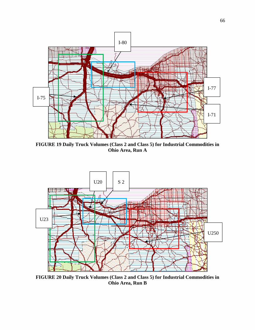
66
FIGURE 19 Daily Truck Volumes (Class 2 and Class 5) for Industrial Commodities in
Ohio Area, Run A
FIGURE 20 Daily Truck Volumes (Class 2 and Class 5) for Industrial Commodities in
Ohio Area, Run B
I-80
I-77
I-71
I-75
S 2
U20
U250
U23
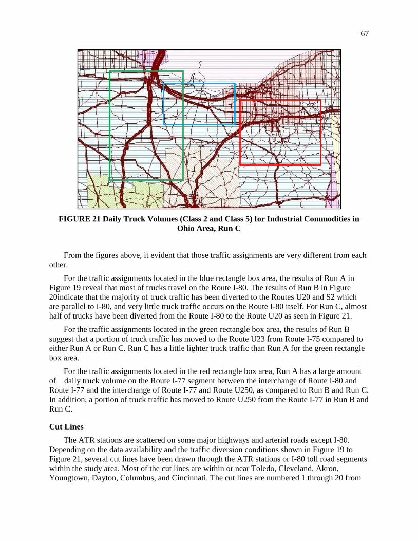
67
FIGURE 21 Daily Truck Volumes (Class 2 and Class 5) for Industrial Commodities in
Ohio Area, Run C
From the figures above, it evident that those traffic assignments are very different from each other.
For the traffic assignments located in the blue rectangle box area, the results of Run A in Figure 19 reveal that most of trucks travel on the Route I-80. The results of Run B in Figure 20indicate that the majority of truck traffic has been diverted to the Routes U20 and S2 which are parallel to I-80, and very little truck traffic occurs on the Route I-80 itself. For Run C, almost half of trucks have been diverted from the Route I-80 to the Route U20 as seen in Figure 21.
For the traffic assignments located in the green rectangle box area, the results of Run B suggest that a portion of truck traffic has moved to the Route U23 from Route I-75 compared to either Run A or Run C. Run C has a little lighter truck traffic than Run A for the green rectangle box area.
For the traffic assignments located in the red rectangle box area, Run A has a large amount of daily truck volume on the Route I-77 segment between the interchange of Route I-80 and Route I-77 and the interchange of Route I-77 and Route U250, as compared to Run B and Run C. In addition, a portion of truck traffic has moved to Route U250 from the Route I-77 in Run B and Run C.
Cut Lines The ATR stations are scattered on some major highways and arterial roads except I-80.
Depending on the data availability and the traffic diversion conditions shown in Figure 19 to Figure 21, several cut lines have been drawn through the ATR stations or I-80 toll road segments within the study area. Most of the cut lines are within or near Toledo, Cleveland, Akron, Youngtown, Dayton, Columbus, and Cincinnati. The cut lines are numbered 1 through 20 from

68
west to east and from north to south. Because the toll pricing appears to have caused much of traffic diversion, most cut lines are drawn across the toll road I-80.
Table 29 summarizes the truck traffic counts passing through the cut lines, which are truck traffic volume results from the three runs and actual truck traffic volume. It is necessary to mention that the truck traffic volume from three runs is the summation of truck counts of two directions. And also, the Ohio Turnpike Authority provides only annual truck traffic volumes, so they needed to be divided by 365 to get annual average daily truck traffic (AADTT). Furthermore, the Ohio turnpike map describes the numbered interchange locations (shown in Figure 22) and the truck traffic volume is given between any two interchange locations. So it is easy to find the truck volume at exactly the same intersected location on the Ohio turnpike map when a cut line intersects the toll road on the road network map.

69
TABLE 29 Truck Traffic Counts Passing through the Cut Lines Cut Line
Station No.
Road Name From To
Run A
Run B
Run C
ATR Station
1 724 U20 S108 S109 20 136 83 1540
34-39 I80 S108 S109 2725 23 971 10945
726 U24 S15 S108 1596 1504 1280 5109 2 603 U20 S109 U23 2 120 66 1870
52-59 I80 S109 U23 2475 21 948 10954
160 U24 U6 U23 1565 1285 1040 5215 3 733 I475 S51 I75 1934 74 541 11090
718 I75 S2 I80 3748 1906 2843 18270
64-71 I80 I75 I280 3183 26 980 12683 4 565 S2 I280 S358 9 1 0 2326
71-81 I80 I75 S51 5263 12 2227 14883
735 U21 I280 U23 220 1567 1169 2680 5 732 I475 U23 S51 1859 9 438 10530
59-64 I80 U20 U24 2585 20 976 11482
605 U20 U24 S25 118 640 191 540 6 71 I475 S2 U20 2160 674 1353 13320
158 I75 S51 S25 3658 798 173 16490
739 I280 I75 S2 2449 4499 6464 10150 7 731 U6 S2 S13 20 1379 293 1380
604 U250 S2 I80 80 36 45 320
110-118 I80 S4 U250 5245 12 2240 14532 8 571 I90 U20 S237 59 121 477 6680
581 I480 S252 S237 1197 939 954 7208
152-161 I80 S10 U42 3610 98 993 10849 9 540 I71 117th St. U42 752 213 268 2860
142 I480 130th St S3 1221 815 951 9132
161-173 I80 S82 I77 3802 81 975 10998 10 575 S2 I90 L King 660 603 619 9940
583 I480 I77 S14 636 548 825 12640
173-180 I80 I77 S8 2307 109 1011 14418

70
TABLE 29 Truck Traffic Counts Passing through the Cut Lines (Continuation) Cutline No.
Station No.
Road Name From To Run
A Run
B Run
C ATR
Station
11 591 U422 S91 S306 224 498 441 2520
148 I480 S91 I80 438 323 367 5210
180-187 I80 S91 S306 2305 130 990 9826
12 766 I480 I271 S91 464 364 377 5480
187-193 I80 S91 I480 2305 130 990 11288
754 I76 S43 S44 1327 2392 1876 11870 13 577 I71 I271 S82 836 479 1228 6747
592 I77 S18 I271 567 131 185 6679
527 I271 S18 S8 930 647 728 10380 14 161-173 I80 S82 I77 3802 81 975 10998
760 S18 I71 I77 96 2074 1101 1834
558 I76 S57 I77 1390 1516 2010 9100 15 543 U422 S534 S5 47 411 365 723
530 I80 I76 S46 3336 2833 2975 16950
554 S11 U62 I80 69 17 165 3420 16 764 S83 S46 S11 58 43 215 2000
762 I80 U422 S11 1760 1567 1429 18000
753 I680 S7 S170 461 156 199 4080 17 545 S49 U36 U40 39 518 459 947
506 I75 S41 U36 3558 1690 2441 17310
714 U33 U68 U36 276 1008 857 3240 18 65 I75 S129 S63 3238 1511 2374 22470
139 I71 I275 S129 4765 1514 2263 24750
523 U22 I71 I275 64 764 314 374 19 744 I670 U62 I270 217 154 196 512
752 I70 U33 S317 2188 1904 2367 11400
502 U33 S104 I270 1200 1699 1881 3440 20 601 I70 I270 S158 1770 510 1020 16030
145 I270 U23 C122 1025 498 826 12420
539 U33 S317 S158 576 1591 1755 3186

71
FIGURE 22 Ohio Turnpike Map
Model Validation Although the traffic assignment outputs have shown a lot of differences in some locations of
Ohio, it is difficult to tell which traffic assignment fits the field data best based on the visual observation of the figures or the values of traffic volume. In order to further validate the assignment model, it is necessary to evaluate the impacts of impedance factors on traffic diversion by analyzing the percentage distribution of truck traffic volume on each cut line from one run to the other, and compare the volume percentage distributions of three runs to the actual traffic volume percentage distribution.
The percentage distribution is obtained by dividing the truck traffic counts of each ATR station on a single cut line by the summation of all volumes for the cut line. The figures in Appendix D present the ATR locations intersected by each cut line and the percentage distribution of actual truck traffic volume on each cut line. The tables in Appendix D corresponding to these figures, respectively show the percentage distribution of truck traffic volume from three runs and the percentage distribution of actual truck traffic volume at the same location on each cut line. The toll road I-80 is highlighted in both figures and tables. It should be noticed that the dots are plotted on the Route I-80 to present the Ohio turnpike count locations which will be considered as the dummy ATR stations and other dots present the State of Ohio ATR stations.
From the figures and tables in Appendix D, it can be concluded that the percentage of actual truck traffic volume at each cut line is close to any percentage of Run A and Run C or somewhere between Runs A and C. Some cases show the percentages of actual truck traffic are similar to the percentages of Run C, such as cut line 10 (shown in Figure 23 with Table 30,

72
which indicates that the tolls on the Route I-80 have affected the total impedances greatly in reality and have caused traffic diversion.
FIGURE 23 Percentage Distribution on Cut Line 10
TABLE 30 Comparison of Percentage Distribution on Cut Line 10
Model Output
Run A Run B Run C ATR Station
18.3% 47.9% 25.2% 26.8%
17.7% 43.4% 33.6% 34.2%
64.0% 8.7% 41.2% 39.0%
Some cases show the percentage of actual truck traffic is between Run A and Run C, such as the cut line 9 (shown in Figure 24 with Table 31), which means that some truck drivers are supposed to have been diverted on the alternate routes to avoid the tolls like the results of Run C but in the real world they are willing to pay the tolls to continue staying on the Route I-80 like the results of Run A.

73
FIGURE 24 Percentage Distribution on Cut Line 9
TABLE 31 Comparison of Percentage Distribution on Cut Line 9
Model Output
Run A Run B Run C ATR Station
13.0% 19.2% 12.2% 12.4%
21.1% 73.5% 43.3% 39.7%
65.8% 7.3% 44.4% 47.8%
Many other cases show that the percentage of actual truck traffic is similar to the percentage of Run A. An example is cut line 6 (shown in Figure 25 with Table 32), in which shows there is no toll road intersected by this cut line. This case suggests that in reality truck drivers choose routes mainly based on the real travel time without giving much consideration to the distance.
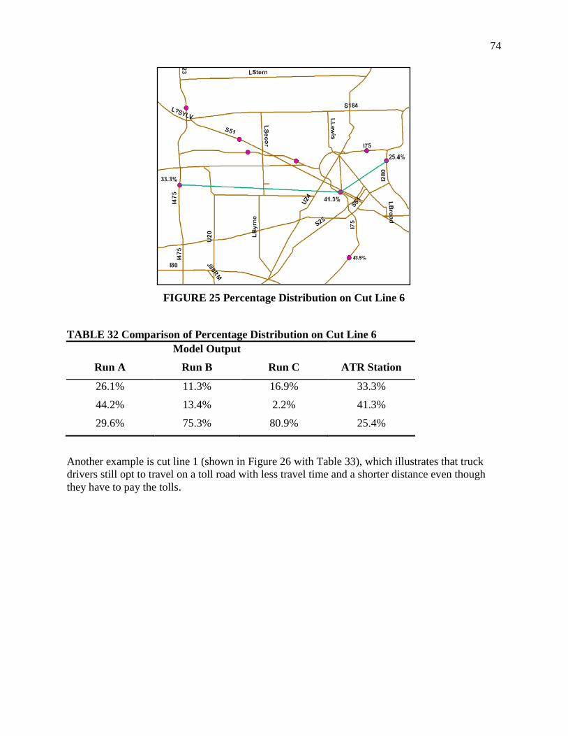
74
FIGURE 25 Percentage Distribution on Cut Line 6
TABLE 32 Comparison of Percentage Distribution on Cut Line 6
Model Output
Run A Run B Run C ATR Station
26.1% 11.3% 16.9% 33.3%
44.2% 13.4% 2.2% 41.3%
29.6% 75.3% 80.9% 25.4%
Another example is cut line 1 (shown in Figure 26 with Table 33), which illustrates that truck drivers still opt to travel on a toll road with less travel time and a shorter distance even though they have to pay the tolls.
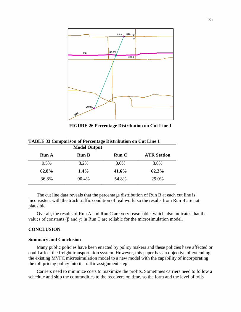
75
FIGURE 26 Percentage Distribution on Cut Line 1
TABLE 33 Comparison of Percentage Distribution on Cut Line 1
Model Output
Run A Run B Run C ATR Station
0.5% 8.2% 3.6% 8.8%
62.8% 1.4% 41.6% 62.2% 36.8% 90.4% 54.8% 29.0%
The cut line data reveals that the percentage distribution of Run B at each cut line is inconsistent with the truck traffic condition of real world so the results from Run B are not plausible.
Overall, the results of Run A and Run C are very reasonable, which also indicates that the values of constants (β and γ) in Run C are reliable for the microsimulation model.
CONCLUSION
Summary and Conclusion Many public policies have been enacted by policy makers and these policies have affected or
could affect the freight transportation system. However, this paper has an objective of extending the existing MVFC microsimulation model to a new model with the capability of incorporating the toll pricing policy into its traffic assignment step.
Carriers need to minimize costs to maximize the profits. Sometimes carriers need to follow a schedule and ship the commodities to the receivers on time, so the form and the level of tolls
76
have unpredictable effects on trucker routing decisions. Most freight models in the past consider only travel time as the path building criterion.
The third part of this paper attempted to estimate the amount of average resting time and average driving time before resting for long distance truck drivers by literature review. However, there was not a single study for specific values of truck drivers’ average resting time and driving time before resting.
The forth part of the paper focused on the values of time and how they can be estimated specifically for different commodities and truck classes. The literature review reveals that there are no studies done for values of time by commodity by truck class in the Mississippi valley region or elsewhere. Thus, a truck cost model developed by Hussein (2010) is modified to calculate truck costs for Scenario One (distance-based costs) and Scenario Two (distance- and time-based costs) by changing some input data. Based on these tuck costs, a linear regression method is then performed to estimate values of time and per-mile cost for five commodities and two truck classes for each Scenario.
By using the value of time by commodity by truck class, the tolls (in dollars) collected from some authorities are converted to extra times (in minutes), which are an input to the simulation. And also, the units of distance are converted to the units of time by using a distance weight (γ/β). After that, an initial test run is performed. The results showed that there is an imbalance of truck volume between Telegraph Rd. and I-75 in southern Michigan, so additional extra times are added to each direction of each surface street to account (roughly) for control delay at the ends of those links.
In the sixth part of this paper, actual truck traffic data in Ohio is assembled. Data comes from ATR stations from the State of Ohio and from counts provided by the Ohio Turnpike Authority.
The seventh part of this paper analyzes the simulation results for the case of three industrial commodities assigned using parameters for motor vehicle parts. Three runs with different assumptions are performed by using the microsimulation model. Run A just used simple travel time as the path building criterion. Run B used parameters that were derived assuming distance-based costs. Run C used parameters that were derived assuming time-based costs. Assignment results showed that truck traffic has diverted from toll roads to the alternative roads at some locations in Run B and Run C.
To further evaluate the assignment model, volumes were compared across cut lines. The comparisons from one run to the other revealed that in response to tolls, truck drivers change their routes when the impedance of the original route exceeds the alternative route’s impedance. With a lower value of travel time truckers may consider alternative routes, whereas when the value of time increases truckers prefer the shortest path to save time. The comparisons of simulation results to actual data showed that the percentage of actual truck traffic volume at each cut line is close to Run A or Run C or somewhere between them. The percentage distribution of volumes from Run B at each cut line is inconsistent with the truck traffic conditions of the real world. This finding suggests that the values of time for motor vehicle parts in Scenario Two are more reliable than those in Scenario One.
77
The simulation results showed that the MVFC microsimulation model can simulate the truck traffic conditions affected by the toll pricing policy by using a linear function of time, distance, and tolls, so long as there are good estimates for values of time.
Recommendations for Future Research For future studies some of the recommendations are stated below:
• The microsimulation model employed in this paper used only two truck classes. This model can be extended to simulate all the truck classes or assign trucks with passenger vehicles on the network. Thus, the simulated traffic conditions would be more realistic. However, this process is more complicated and difficult since the scale of the network of ten states is so large.
• One desirable improvement can be to allow the microsimulation model to deal with the dynamic pricing problem. This paper used the average toll rates of different time periods such as day time and overnight, peak times and off-peak times. Being allowed to price tolls dynamically, the model would be able to charge the users different toll rates for different time periods, which might result in further improvements in traffic forecasts.
• Five indicative commodities are used for the Mississippi Valley region. This paper analyzed the simulation results only for three industrial commodities, but used parameters for motor vehicle parts. For the future work, we can simulate all five commodities separately and then compare the results to see the impacts of different commodities on truck traffic diversion. It would also be possible to simulate all five commodities with their own parameters.
• When solving the intersection control problem, we assumed that 0.5 minutes of extra time are added to each direction of each surface street to account (roughly) for control delay at the ends of those links. In the future, the model can be modified through comprehensive research on speed adjustments.
• The static traffic assignments have been tested in this paper so we need to fully test dynamic traffic assignments in the near future.
• Only toll pricing policy has been incorporated into the current microsimulation model so for future work many other public policies should be tested, as described on Table 1.
ACKNOWLEDGEMENTS This study was funded by the National Center for Freight & Infrastructure Research &
Education (CFIRE), a university research center of the U.S. Department of Transportation. The truck cost model used in this study was provided by Mazen Hussein. The actual traffic data analyzed in this study was provided by the Ohio Department of Transportation.

78
REFERENCES
1. Outwater, M., Kitchen, M., (2008), “Value of Time for Travel Forecasting and Benefits Analysis”, Retrieved October 2010, from http://www.psrc.org/assets/1820/ValueofTimeMemo-updated.pdf
2. Outwater, M., Kitchen, M., Ardussi, S., Bassok, A., Rossi, S., (2009), “Travel Model Improvements for the Congestion Management Process and Long Range Transportation Plan Update”, Retrieved October 2010, from http://www.psrc.org/assets/3129/Final_Report_PSRC_Travel_Model_Freight.pdf
3. Killough, K., (2008), “Value Analysis of Truck Toll Lanes in Southern California”, Transportation Research Board 87th Annual Meeting, pp.11.
4. Concas, S., Kolpakov, A., (2009),“Florida Department of Transportation, Synpaper of Research on Value of Time and Value of Reliability”, Retrieved October 2010, from http://www.nctr.usf.edu/pdf/77806.pdf
5. Kawamura, K., (2003), “Perceived Benefits of Congestion Pricing for Trucks”, Transportation Research Record, Issue 1833, pp. 59-65
6. Kruesi, F., (1997), “The Value of Saving Travel Time: Departmental Guidance for Conducting Economic Evaluations”, Retrieved October 2010, from http://ostpxweb.dot.gov/policy/Data/VOT97guid.pdf
7. ATRI, (2010), “An Analysis of the Operational Costs of Trucking”, Transportation Research Board 89th Annual Meeting, pp.17.
8. Smalkoski, B., Levinson, D., (2005), “Value of Time for Commercial Vehicle Operators in Minnesota”, Journal of the Transportation Research Forum 44:1 pp. 89-102.
9. Fowkes, T., (2001), “Values of Time for Road Commercial Vehicles”, Retrieved October 2010, from http://eprints.whiterose.ac.uk/2063/1/ITS38_WP563_uploadable.pdf
10. Victoria Transport Policy Institute, (2010),“Transportation Cost and Benefit Analysis II – Travel Time Costs”, Retrieved October 2010, from http://trainsnotlanes.info/Documents/tca0502.pdf
11. Wigan, M., Rockliffe, N., Thoresen, T., Tsolakis, D., (2000), “Valuing Long-Haul and Metropolitan Freight Travel Time and Reliability”, Retrieved October 2010, from http://www.bts.gov/publications/journal_of_transportation_and_statistics/volume_03_number_03/paper_06/index.html
12. Kurri, J., Sirkiä, A., Mikola, J., (2007), “Value of Time in Freight Transport in Finland”, Transportation Research Record, Vol. 1725 / 2000, pp. 26-30.
13. Ismail, K., Sayed, T., Lim, C., (2009), “A Study of the Commercial Vehicle Value of Time

79
for Operation at Border Crossings”, Retrieved October 2010, from http://www.tac-atc.ca/english/resourcecentre/readingroom/conference/conf2009/pdf/Ismail2.pdf
14. Montana Department of Transportation, (2005), “Montana Highway Reconfiguration Study”, Retrieved October 2010, from http://www.mdt.mt.gov/research/docs/reconfig/final_report.pdf
15. Berwick, M., Dooley, F., (1997), “Truck Costs for Owner/Operators”, Research report, North Dakota State University, Fargo.
16. Berwick, M., Farooq, M., (2003), “Truck Costing Model for Transportation Managers. Research report”, North Dakota State University, Fargo.
17. Ergun, O., Kuyzu, G., Savelsbergh, M., (2007), “Reducing Truckload Transportation Costs through Collaboration”, Transportation Science, Vol.41, pp. 206-221.
18. Hussein, M., Petering, M., Horowitz, A., (2010), “A Policy-Oriented Cost Model for Shipping Commodities by Truck”, National Center for Freight & Infrastructure Research & Education, Center for Urban Transportation Studies, University of Wisconsin-Milwaukee.
19. U.S. DOT Federal Highway Administration, (2007), “FAF2 Technical Documentation”, FHWA, Retrieved October 2010, from http://ops.fhwa.dot.gov/freight/freight_analysis/faf/faf2_reports/reports9/index.htm
20. U.S. DOT Federal Highway Administration, (2000),“Comprehensive Truck Size and Weight (CTS&W) Study”, Retrieved October 2010, from http://www.fhwa.dot.gov/reports/tswstudy/Vol2-Chapter3.pdf
21. U.S. DOT Federal Highway Administration, “Truck Size and Weight”, Retrieved October 2010, from http://ops.fhwa.dot.gov/freight/sw/index.htm
22. Transportation Research Board, (2003), “Review of Truck Characteristics as Factors in Roadway Design”, NCHRP Report 505, Retrieved October 2010, from http://onlinepubs.trb.org/onlinepubs/nchrp/nchrp_rpt_505.pdf
23. Transportation Research Board, (2010), “Impacts of Public Policy on the Freight Transportation System”, NCFRP Report 6, Retrieved December 2010, from http://onlinepubs.trb.org/onlinepubs/ncfrp/ncfrp_rpt_006.pdf
24. Transportation Research Board, (2008), “Forecasting Statewide Freight Toolkit”, NCHRP Report 606, Retrieved September 2010, from http://onlinepubs.trb.org/onlinepubs/nchrp/nchrp_rpt_606.pdf
25. Transportation Research Board, (2008), “Forecasting Metropolitan Commercial and Freight Travel”, NCHRP Synpaper 384, Retrieved September 2010, from http://onlinepubs.trb.org/onlinepubs/nchrp/nchrp_syn_384.pdf

80
26. Transportation Research Board, (2010), “Advanced Practices in Traveling Forecasting”, NCHRP Synpaper 406, Retrieved September 2010, from http://onlinepubs.trb.org/onlinepubs/nchrp/nchrp_syn_406.pdf
27. U.S. DOT Federal Highway Administration, (2007), “Quick Response Freight Manual II”, Retrieved September 2010, from http://ops.fhwa.dot.gov/freight/publications/qrfm2/qrfm.pdf
28. Oak Ridge National Laboratory, (2010), “Network Assignment of Highway Truck Traffic in FAF3”, Retrieved January 2011, from http://cta-gis.ornl.gov/faf/Data/FAF_3_network_assignment_executive_summary.pdf
29. Horowitz, A., (2010), “Microsimulation of Commodity Flow in the Mississippi Valley Region”, National Center for Freight & Infrastructure Research &Education, Center for Urban Transportation Studies, University of Wisconsin-Milwaukee.
30. Ohio Turnpike Authority website, Retrieved February 2011, from http://www.ohioturnpike.org/
31. Melendez, M., (2010), “Transshipment Tour Structures for the Ontario Commercial Vehicle Survey”, University of Wisconsin-Milwaukee.
32. Federal Highway Administration, “Highway Control Systems Handbook”, Retrieved March 2011, from http://ops.fhwa.dot.gov/publications/fhwahop06006/chapter_3p1.htm
33. Horowitz, A., (1987), “Applications of the General Network Editor”, Microcomputer Applications in Transportation II, Proceedings of the North American Conference on Microcomputers in Transportation, pp. 262-269
34. U.S. DOT, Transport Canada, and Trucking Research Institute, (1996), “Commercial Motor Vehicle Driver Fatigue and Alertness Study”, Retrieved July 2010, from http://www.fatigueauvolant.ca/documents/1996_11_00_12876e.pdf
35. Hanowski, R., Hickman, J., Fumero, M., Olson, R., Dingus, T., (2007), “The Sleep of Commercial Vehicle Drivers under the 2003 Hours of Service Regulations”, Accid Anal Prev, Vol. 39, No. 6, pp. 1140-1145
36. Baas, P., Charlton S., (2000), “Fatigue, Work-Rest Cycles, and Psychomotor performance of New Zealand Truck Drivers”, Retrieved July 2010, from http://www.psychology.org.nz/cms_show_download.php?id=692
37. Mccartt, A., Hellinga, L., and Solomon, M., (2008), “Work Schedules of Long-Distance Truck Drivers before and after 2004 Hours-of-Service Rule Change”, Traffic InjPrev, Vol. 9, No. 3, pp. 201-210(10)
38. Williamson, A., Feyer, A., Friswell, R., Leslie, D., (1992), “Strategies to Combat Fatigue in the Long Distance Road Transport Industry”,National Occupational Health and Safety Commission, pp. 158-159
81
39. Philip, P., Taillard, J., Léger, D., Diefenbach, K., Akerstedt, T.,Bioulac, B.,Guilleminault, C., (2002), “Work and Rest Sleep Schedules of 227 European Truck Drivers”, Sleep Medicine, Vol. 3, No. 6, pp. 507-511
40. FMCSA of US DOT, (2005), “Hours of Service of Drivers”, Retrieved July 2010, from http://www.fmcsa.dot.gov/rules-regulations/administration/rulemakings/final/05-16498-HOS-Final-Rule-8-25-05.htm
41. Mitler, M., Miller, J., Lipsitz, J., Walsh, J., and Wylie, C., (1997), “The Sleep of Long-Haul Truck Drivers”, N Engl J Med, Vol. 337 (11), pp. 755-61
42. McCartt, A., Rohrbaugh, J., Hammer, M., Fuller, S., (2000), “ Factors Associated with Falling Asleep at the Wheel among Long-Distance Truck Drivers”, Accident Analysis & Prevention, Vol. 32, No. 4, pp. 493-504
43. Braver, E., Preusser, C., Preusser, D., Baum, H., Beilock, R., and Ulmer, R., (1992), “Long Hours and Fatigue: A Survey of Tractor-Trailer Drivers”, Public Health Policy, Vol.13, No. 3, pp. 341-366.
44. Rodier, C., Shaheen, S., Allen, D., and Dix, B., (2010), “Commercial Vehicle Parking in California: Exploratory Evaluation of the Problem and Solutions”, PATH Research Report, pp. 1-29
45. Beltemacchi, P., Rohter, L., Selinksky, J., Manning, T., (2008), “Truckers’ Park/Rest Facility Study”, Civil Engineering Studies, Illinois Center for Transportation Series, No. 08-018, pp. 1-49
46. PRR, WSDOT, (2008), “Washington State Truck Parking Survey Summary Report”, Retrieved August 2010, from http://www.wsdot.wa.gov/NR/rdonlyres/E1D2034B-06B3-4CA4-96A5-B47C0A79A1DB/0/WSDOTTruckParkingSurveyApril2008_web.pdf
47. Chen, K., Pecheux, K., Farbry J., Fleger, S., (2002), “Commercial Vehicle Driver Survey: Assessment of Parking Needs and Preferences”, Retrieved August 2010, from http://www.fhwa.dot.gov/publications/research/safety/01160/index.cfm
48. Chatterjee, A., and Wegmann, F., (2000), “Overnight Truck Parking Along Tennessee’s Interstate Highways and Rest Areas”, Transportation Research Record, No. 1734, pp. 64-68
49. Garber,N., and Wang H., (2004), “Estimation of the Demand for Commercial Truck Parking on Interstate Highways in Virginia”, Retrieved August 2010, from http://www.virginiadot.org/vtrc/main/online_reports/pdf/04-r10.pdf
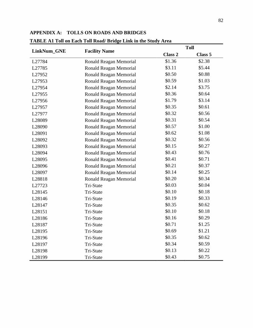
82
APPENDIX A: TOLLS ON ROADS AND BRIDGES TABLE A1 Toll on Each Toll Road/ Bridge Link in the Study Area
LinkNum_GNE Facility Name Toll
Class 2 Class 5 L27784 Ronald Reagan Memorial $1.36 $2.38 L27785 Ronald Reagan Memorial $3.11 $5.44 L27952 Ronald Reagan Memorial $0.50 $0.88 L27953 Ronald Reagan Memorial $0.59 $1.03 L27954 Ronald Reagan Memorial $2.14 $3.75 L27955 Ronald Reagan Memorial $0.36 $0.64 L27956 Ronald Reagan Memorial $1.79 $3.14 L27957 Ronald Reagan Memorial $0.35 $0.61 L27977 Ronald Reagan Memorial $0.32 $0.56 L28089 Ronald Reagan Memorial $0.31 $0.54 L28090 Ronald Reagan Memorial $0.57 $1.00 L28091 Ronald Reagan Memorial $0.62 $1.08 L28092 Ronald Reagan Memorial $0.32 $0.56 L28093 Ronald Reagan Memorial $0.15 $0.27 L28094 Ronald Reagan Memorial $0.43 $0.76 L28095 Ronald Reagan Memorial $0.41 $0.71 L28096 Ronald Reagan Memorial $0.21 $0.37 L28097 Ronald Reagan Memorial $0.14 $0.25 L28818 Ronald Reagan Memorial $0.20 $0.34 L27723 Tri-State $0.03 $0.04 L28145 Tri-State $0.10 $0.18 L28146 Tri-State $0.19 $0.33 L28147 Tri-State $0.35 $0.62 L28151 Tri-State $0.10 $0.18 L28186 Tri-State $0.16 $0.29 L28187 Tri-State $0.71 $1.25 L28195 Tri-State $0.69 $1.21 L28196 Tri-State $0.35 $0.62 L28197 Tri-State $0.34 $0.59 L28198 Tri-State $0.13 $0.22 L28199 Tri-State $0.43 $0.75

83
TABLE A1 Toll on Each Toll Road/ Bridge Link in the Study Area (Continuation)
LinkNum_GNE Facility Name Toll
Class 2 Class 5 L28200 Tri-State $0.23 $0.40 L28201 Tri-State $0.03 $0.04 L28202 Tri-State $0.13 $0.22 L28203 Tri-State $0.06 $0.11 L28204 Tri-State $0.08 $0.13 L28205 Tri-State $0.23 $0.40 L28297 Tri-State $0.23 $0.40 L28298 Tri-State $0.31 $0.55 L28372 Tri-State $0.61 $1.08 L28373 Tri-State $0.25 $0.44 L28374 Tri-State $0.06 $0.11 L28375 Tri-State $0.18 $0.31 L28376 Tri-State $0.25 $0.44 L28377 Tri-State $0.13 $0.22 L28378 Tri-State $0.46 $0.81 L28379 Tri-State $0.48 $0.84 L28380 Tri-State $0.14 $0.24 L28381 Tri-State $0.30 $0.53 L28382 Tri-State $0.36 $0.64 L28383 Tri-State $0.65 $1.14 L28384 Tri-State $0.33 $0.57 L28385 Tri-State $0.13 $0.22 L28386 Tri-State $0.21 $0.37 L28387 Tri-State $0.75 $1.32 L28388 Tri-State $0.19 $0.33 L28278 Jane Addams Memorial $0.57 $0.99 L28279 Jane Addams Memorial $0.73 $1.27 L28280 Jane Addams Memorial $0.36 $0.63 L28281 Jane Addams Memorial $0.46 $0.80 L28282 Jane Addams Memorial $0.34 $0.59 L28283 Jane Addams Memorial $0.45 $0.78 L28284 Jane Addams Memorial $0.19 $0.33 L28414 Jane Addams Memorial $0.12 $0.21 L28449 Jane Addams Memorial $0.26 $0.45 L28462 Jane Addams Memorial $0.41 $0.71 L28463 Jane Addams Memorial $1.65 $2.87
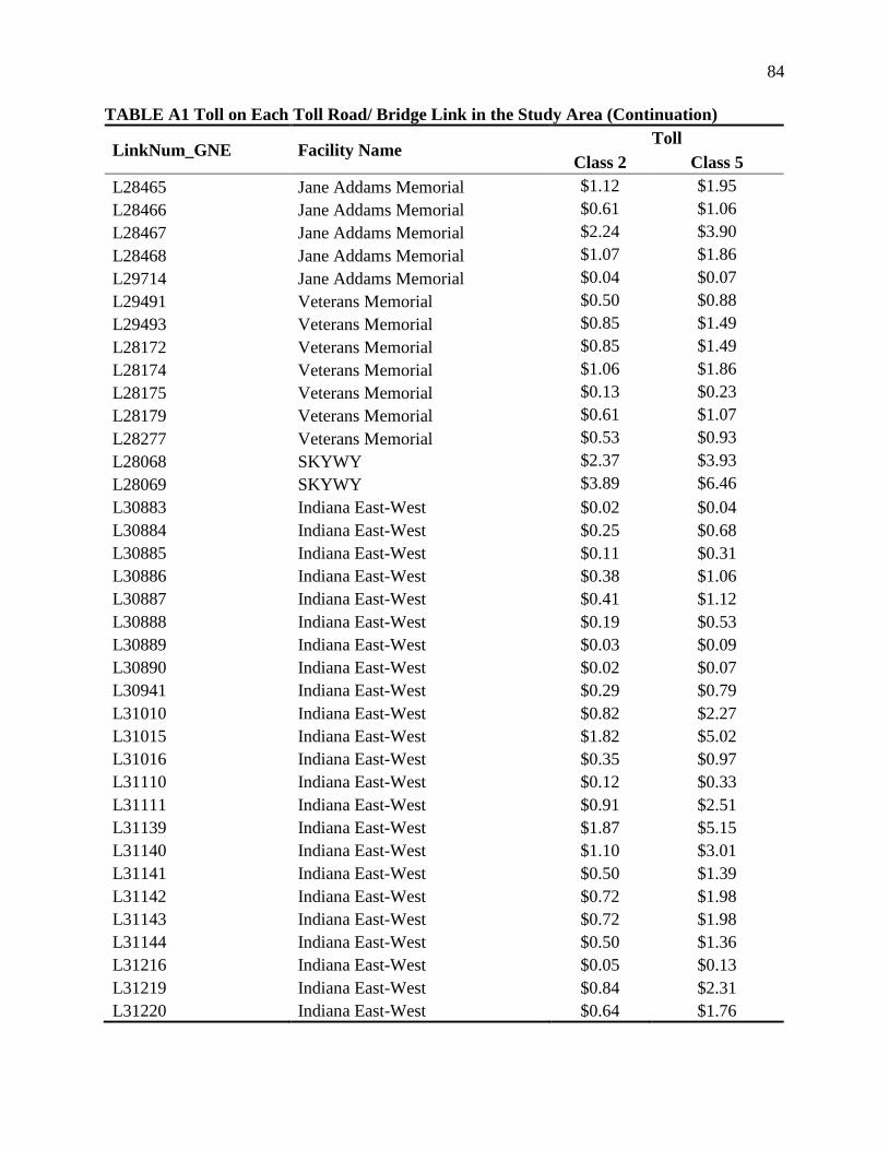
84
TABLE A1 Toll on Each Toll Road/ Bridge Link in the Study Area (Continuation)
LinkNum_GNE Facility Name Toll
Class 2 Class 5 L28465 Jane Addams Memorial $1.12 $1.95 L28466 Jane Addams Memorial $0.61 $1.06 L28467 Jane Addams Memorial $2.24 $3.90 L28468 Jane Addams Memorial $1.07 $1.86 L29714 Jane Addams Memorial $0.04 $0.07 L29491 Veterans Memorial $0.50 $0.88 L29493 Veterans Memorial $0.85 $1.49 L28172 Veterans Memorial $0.85 $1.49 L28174 Veterans Memorial $1.06 $1.86 L28175 Veterans Memorial $0.13 $0.23 L28179 Veterans Memorial $0.61 $1.07 L28277 Veterans Memorial $0.53 $0.93 L28068 SKYWY $2.37 $3.93 L28069 SKYWY $3.89 $6.46 L30883 Indiana East-West $0.02 $0.04 L30884 Indiana East-West $0.25 $0.68 L30885 Indiana East-West $0.11 $0.31 L30886 Indiana East-West $0.38 $1.06 L30887 Indiana East-West $0.41 $1.12 L30888 Indiana East-West $0.19 $0.53 L30889 Indiana East-West $0.03 $0.09 L30890 Indiana East-West $0.02 $0.07 L30941 Indiana East-West $0.29 $0.79 L31010 Indiana East-West $0.82 $2.27 L31015 Indiana East-West $1.82 $5.02 L31016 Indiana East-West $0.35 $0.97 L31110 Indiana East-West $0.12 $0.33 L31111 Indiana East-West $0.91 $2.51 L31139 Indiana East-West $1.87 $5.15 L31140 Indiana East-West $1.10 $3.01 L31141 Indiana East-West $0.50 $1.39 L31142 Indiana East-West $0.72 $1.98 L31143 Indiana East-West $0.72 $1.98 L31144 Indiana East-West $0.50 $1.36 L31216 Indiana East-West $0.05 $0.13 L31219 Indiana East-West $0.84 $2.31 L31220 Indiana East-West $0.64 $1.76
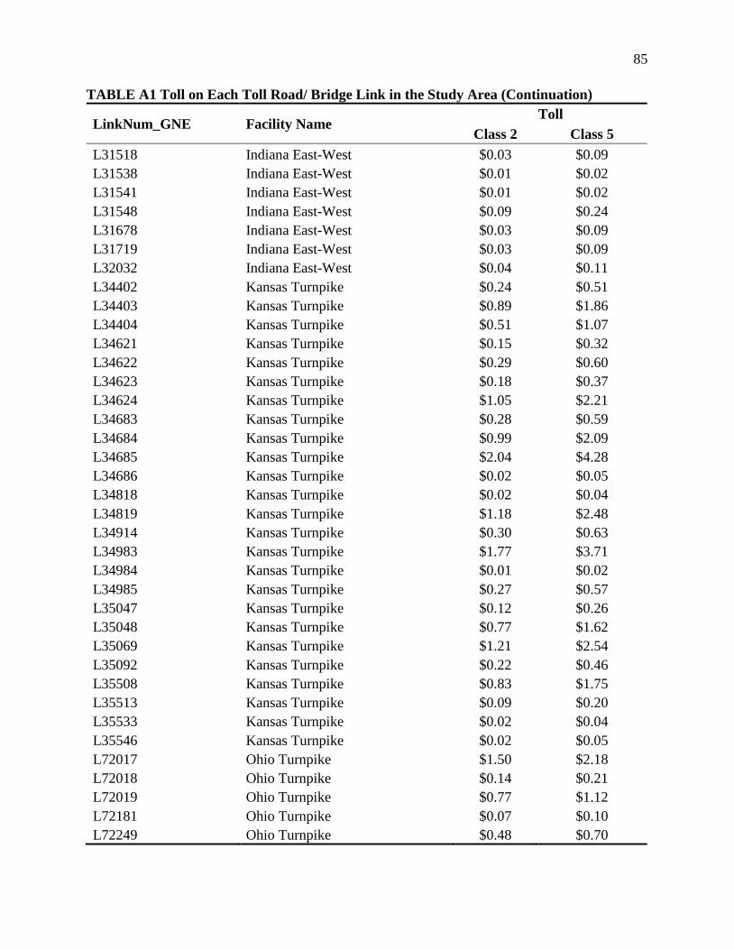
85
TABLE A1 Toll on Each Toll Road/ Bridge Link in the Study Area (Continuation)
LinkNum_GNE Facility Name Toll
Class 2 Class 5 L31518 Indiana East-West $0.03 $0.09 L31538 Indiana East-West $0.01 $0.02 L31541 Indiana East-West $0.01 $0.02 L31548 Indiana East-West $0.09 $0.24 L31678 Indiana East-West $0.03 $0.09 L31719 Indiana East-West $0.03 $0.09 L32032 Indiana East-West $0.04 $0.11 L34402 Kansas Turnpike $0.24 $0.51 L34403 Kansas Turnpike $0.89 $1.86 L34404 Kansas Turnpike $0.51 $1.07 L34621 Kansas Turnpike $0.15 $0.32 L34622 Kansas Turnpike $0.29 $0.60 L34623 Kansas Turnpike $0.18 $0.37 L34624 Kansas Turnpike $1.05 $2.21 L34683 Kansas Turnpike $0.28 $0.59 L34684 Kansas Turnpike $0.99 $2.09 L34685 Kansas Turnpike $2.04 $4.28 L34686 Kansas Turnpike $0.02 $0.05 L34818 Kansas Turnpike $0.02 $0.04 L34819 Kansas Turnpike $1.18 $2.48 L34914 Kansas Turnpike $0.30 $0.63 L34983 Kansas Turnpike $1.77 $3.71 L34984 Kansas Turnpike $0.01 $0.02 L34985 Kansas Turnpike $0.27 $0.57 L35047 Kansas Turnpike $0.12 $0.26 L35048 Kansas Turnpike $0.77 $1.62 L35069 Kansas Turnpike $1.21 $2.54 L35092 Kansas Turnpike $0.22 $0.46 L35508 Kansas Turnpike $0.83 $1.75 L35513 Kansas Turnpike $0.09 $0.20 L35533 Kansas Turnpike $0.02 $0.04 L35546 Kansas Turnpike $0.02 $0.05 L72017 Ohio Turnpike $1.50 $2.18 L72018 Ohio Turnpike $0.14 $0.21 L72019 Ohio Turnpike $0.77 $1.12 L72181 Ohio Turnpike $0.07 $0.10 L72249 Ohio Turnpike $0.48 $0.70

86
TABLE A1 Toll on Each Toll Road/ Bridge Link in the Study Area (Continuation)
LinkNum_GNE Facility Name Toll
Class 2 Class 5 L72250 Ohio Turnpike $0.21 $0.30 L72251 Ohio Turnpike $0.04 $0.06 L72252 Ohio Turnpike $1.07 $1.55 L72253 Ohio Turnpike $1.25 $1.82 L72254 Ohio Turnpike $0.78 $1.14 L72256 Ohio Turnpike $0.76 $1.10 L72257 Ohio Turnpike $0.78 $1.14 L72258 Ohio Turnpike $1.65 $2.40 L72259 Ohio Turnpike $0.68 $0.99 L72260 Ohio Turnpike $0.36 $0.53 L72261 Ohio Turnpike $0.08 $0.11 L72271 Ohio Turnpike $0.06 $0.08 L72467 Ohio Turnpike $0.55 $0.80 L72468 Ohio Turnpike $0.79 $1.15 L72469 Ohio Turnpike $2.20 $3.20 L72470 Ohio Turnpike $2.97 $4.32 L72478 Ohio Turnpike $1.49 $2.16 L72479 Ohio Turnpike $2.35 $3.42 L72480 Ohio Turnpike $1.98 $2.88 L72481 Ohio Turnpike $0.74 $1.07 L73022 Ohio Turnpike $0.03 $0.05 L73111 Ohio Turnpike $2.65 $3.86 L73357 Ohio Turnpike $0.31 $0.45 L74091 Ohio Turnpike $0.03 $0.05 L74095 Ohio Turnpike $0.07 $0.10 L74177 Ohio Turnpike $0.02 $0.03 L74178 Ohio Turnpike $0.03 $0.05 L74179 Ohio Turnpike $0.07 $0.10 L74230 Ohio Turnpike $0.03 $0.05 L74238 Ohio Turnpike $0.02 $0.03 L74314 Ohio Turnpike $0.03 $0.05 L74350 Ohio Turnpike $0.03 $0.05 L74360 Ohio Turnpike $0.04 $0.06 L74483 Ohio Turnpike $0.04 $0.06 L74484 Ohio Turnpike $0.01 $0.02 L74556 Ohio Turnpike $0.04 $0.06 L74557 Ohio Turnpike $0.03 $0.05

87
TABLE A1 Toll on Each Toll Road/ Bridge Link in the Study Area (Continuation)
LinkNum_GNE Facility Name Toll
Class 2 Class 5 L74581 Ohio Turnpike $0.06 $0.08 L74582 Ohio Turnpike $0.07 $0.10 L26881 Wabash Memorial Bridge $0.62 $0.95 L29983 Wabash Memorial Bridge $0.33 $0.50 L28927 Fort Madison Bridge $2.77 $5.54 L33612 Fort Madison Bridge $1.23 $2.46 L44627 Mackinac Bridge $13.50 $22.50 L46406 Detroit-Windsor Tunnel $1.69 $2.11 L29993 New Harmony Bridge $0.08 $0.16 L26882 New Harmony Bridge $1.42 $2.84 L32431 Plattsmouth Bridge $2.25 $2.75 L33336 Bellevue Bridge $3.00 $5.00 L33669 Burt County Bridge $2.50 $5.00 L46403 International Bridge $4.70 $7.83 L109909 International Bridge $7.30 $12.17 L46404 Blue Water Bridge $2.97 $4.95 L109910 Blue Water Bridge $6.78 $11.30 L109911 Ambassador Bridge $5.38 $8.97 L46405 Ambassador Bridge $2.56 $4.26

APPENDIX B: FIGURES ABOUT RELATIONSHIP OF COST AND TIME, AND OF COST AND DISTANCE FOR SCENARIO ONE
FIGURE B1 Linear Relationship of Cost/Time (Corn, Class 2, Scenario One) FIGURE B2 Linear Relationship of Cost/Distance (Corn, Class 2, Scenario One)
FIGURE B3 Linear Relationship of Cost/Time (Corn, Class 5, Scenario One) FIGURE B4 Linear Relationship of Cost/Distance (Corn, Class 5, Scenario One)
y = 6.8007x + 371.23R² = 0.9428
380390400410420430440450
0.00 2.00 4.00 6.00 8.00 10.00 12.00
Cost
($)
Traveling Time (h)
y = 1.8601x + 13.218R² = 0.9989
0
50
100
150
200
250
300
0 50 100 150
Cost
($)
Distance (mile)
y = 14.16x + 400.08R² = 0.9378
390
440
490
540
590
0.00 2.00 4.00 6.00 8.00 10.00 12.00
Cost
($)
Traveling Time (h)
y = 1.9508x + 32.64R² = 0.9981
050
100150200250300350
0 50 100 150Co
st ($
)
Distance (mile)
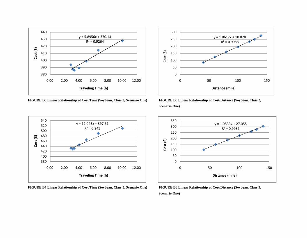
FIGURE B5 Linear Relationship of Cost/Time (Soybean, Class 2, Scenario One) FIGURE B6 Linear Relationship of Cost/Distance (Soybean, Class 2,
Scenario One)
FIGURE B7 Linear Relationship of Cost/Time (Soybean, Class 5, Scenario One) FIGURE B8 Linear Relationship of Cost/Distance (Soybean, Class 5,
Scenario One)
y = 5.8956x + 370.13R² = 0.9264
380
390
400
410
420
430
440
0.00 2.00 4.00 6.00 8.00 10.00 12.00
Cost
($)
Traveling Time (h)
y = 1.8612x + 10.828R² = 0.9988
0
50
100
150
200
250
300
0 50 100 150
Cost
($)
Distance (mile)
y = 12.043x + 397.51R² = 0.945
380400420440460480500520540
0.00 2.00 4.00 6.00 8.00 10.00 12.00
Cost
($)
Traveling Time (h)
y = 1.9533x + 27.055R² = 0.9987
0
50
100
150
200
250
300
350
0 50 100 150Co
st ($
)
Distance (mile)

FIGURE B9 Linear Relationship of Cost/Time (Dairy, Class 2, Scenario One) FIGURE B10 Linear Relationship of Cost/Distance (Dairy, Class 2, Scenario One)
FIGURE B11 Linear Relationship of Cost/Time (Dairy, Class 5, Scenario One) FIGURE B12 Linear Relationship of Cost/Distance (Dairy, Class 5, Scenario One)
y = 10.289x + 389.48R² = 1
410420430440450460470480490500
0.00 2.00 4.00 6.00 8.00 10.00 12.00
Cost
($)
Traveling Time (h)
y = 1.9475x + 20.571R² = 1
0
50
100
150
200
250
300
350
0 50 100 150
Cost
($)
Distance (mile)
y = 22.778x + 398.04R² = 0.9823
400
450
500
550
600
650
0.00 2.00 4.00 6.00 8.00 10.00 12.00
Cost
($)
Traveling Time (h)
y = 1.9528x + 48.808R² = 0.9986
0
50
100
150
200
250
300
350
0 50 100 150A
xis
Titl
eDistance (mile)

FIGURE B13 Linear Relationship of Cost/Time (Plastics, Class 2, Scenario One) FIGURE B14 Linear Relationship of Cost/Distance (Plastics, Class 2,
Scenario One)
FIGURE B15 Linear Relationship of Cost/Time (Plastics, Class 5, Scenario One) FIGURE B16 Linear Relationship of Cost/Distance (Plastics, Class 5,
Scenario One)
y = 3.3894x + 366.68R² = 0.739
370
375
380
385
390
395
400
405
0.00 2.00 4.00 6.00 8.00 10.00 12.00
Cost
($)
Traveling Time (h)
y = 1.8622x + 4.2091R² = 0.9982
0
50
100
150
200
250
300
0 50 100 150
Cost
($)
Distance (mile)
y = 11.016x + 396.25R² = 0.9483
420
440
460
480
500
520
0.00 2.00 4.00 6.00 8.00 10.00 12.00
Cost
($)
Traveling Time (h)
y = 1.9545x + 24.347R² = 0.9989
0
50
100
150
200
250
300
350
0 50 100 150Co
st ($
)
Distance (mile)

FIGURE B17 Linear Relationship of Cost/Time (Motor Vehicle Parts, Class 2, FIGURE B18 Linear Relationship of Cost/Distance (Motor Vehicle Parts,
Scenario One) Class 2, Scenario One)
FIGURE B19 Linear Relationship of Cost/Time (Motor Vehicle Parts, Class 5, FIGURE B20 Linear Relationship of Cost/Distance (Motor Vehicle Parts,
Scenario One) Class 5, Scenario One)
y = 4.7923x + 357.51R² = 0.882
365370375380385390395400405410
0.00 2.00 4.00 6.00 8.00 10.00 12.00
Cost
($)
Traveling Time (h)
y = 1.8616x + 7.9178R² = 0.9986
0
50
100
150
200
250
300
0 50 100 150
Cost
($)
Distance (mile)
y = 10.566x + 395.71R² = 0.9496
420
440
460
480
500
520
0.00 2.00 4.00 6.00 8.00 10.00 12.00
Cost
($)
Traveling Time (h)
y = 1.9551x + 23.156R² = 0.999
0
50
100
150
200
250
300
350
0 50 100 150Co
st ($
)
Distance (mile)

APPENDIX C: FIGURES ABOUT RELATIONSHIP OF COST/TIME, AND OF COST/DISTANCE FOR SCENARIO TWO
FIGURE C1 Linear Relationship of Cost/Time (Corn, Class 2, Scenario Two) FIGURE C2 Linear Relationship of Cost/Distance (Corn, Class 2, Scenario Two)
FIGURE C3 Linear Relationship of Cost/Time (Corn, Class 5, Scenario Two) FIGURE C4 Linear Relationship of Cost/Distance (Corn, Class 5, Scenario Two)
y = 29.506x + 211.33R² = 0.9968
250
300
350
400
450
500
550
0.00 2.00 4.00 6.00 8.00 10.00 12.00
Cost
($)
Traveling Time (h)
y = 1.0607x + 58.627R² = 0.9967
0
50
100
150
200
250
0 50 100 150
Cost
($)
Distance (mile)
y = 36.891x + 239.81R² = 0.9903
150
250
350
450
550
650
0.00 2.00 4.00 6.00 8.00 10.00 12.00
Cost
($)
Traveling Time (h)
y = 1.1494x + 78.105R² = 0.9945
0
50
100
150
200
250
300
0 50 100 150
Cost
($)
Distance (mile)
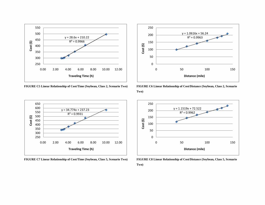
FIGURE C5 Linear Relationship of Cost/Time (Soybean, Class 2, Scenario Two) FIGURE C6 Linear Relationship of Cost/Distance (Soybean, Class 2, Scenario
Two)
FIGURE C7 Linear Relationship of Cost/Time (Soybean, Class 5, Scenario Two) FIGURE C8 Linear Relationship of Cost/Distance (Soybean, Class 5, Scenario
Two)
y = 28.6x + 210.22R² = 0.9966
250
300
350
400
450
500
550
0.00 2.00 4.00 6.00 8.00 10.00 12.00
Cost
($)
Traveling Time (h)
y = 1.0616x + 56.24R² = 0.9963
0
50
100
150
200
250
0 50 100 150
Cost
($)
Distance (mile)
y = 34.774x + 237.23R² = 0.9931
250300350400450500550600650
0.00 2.00 4.00 6.00 8.00 10.00 12.00
Cost
($)
Traveling Time (h)
y = 1.1519x + 72.522R² = 0.9962
0
50
100
150
200
250
0 50 100 150Co
st ($
)
Distance (mile)
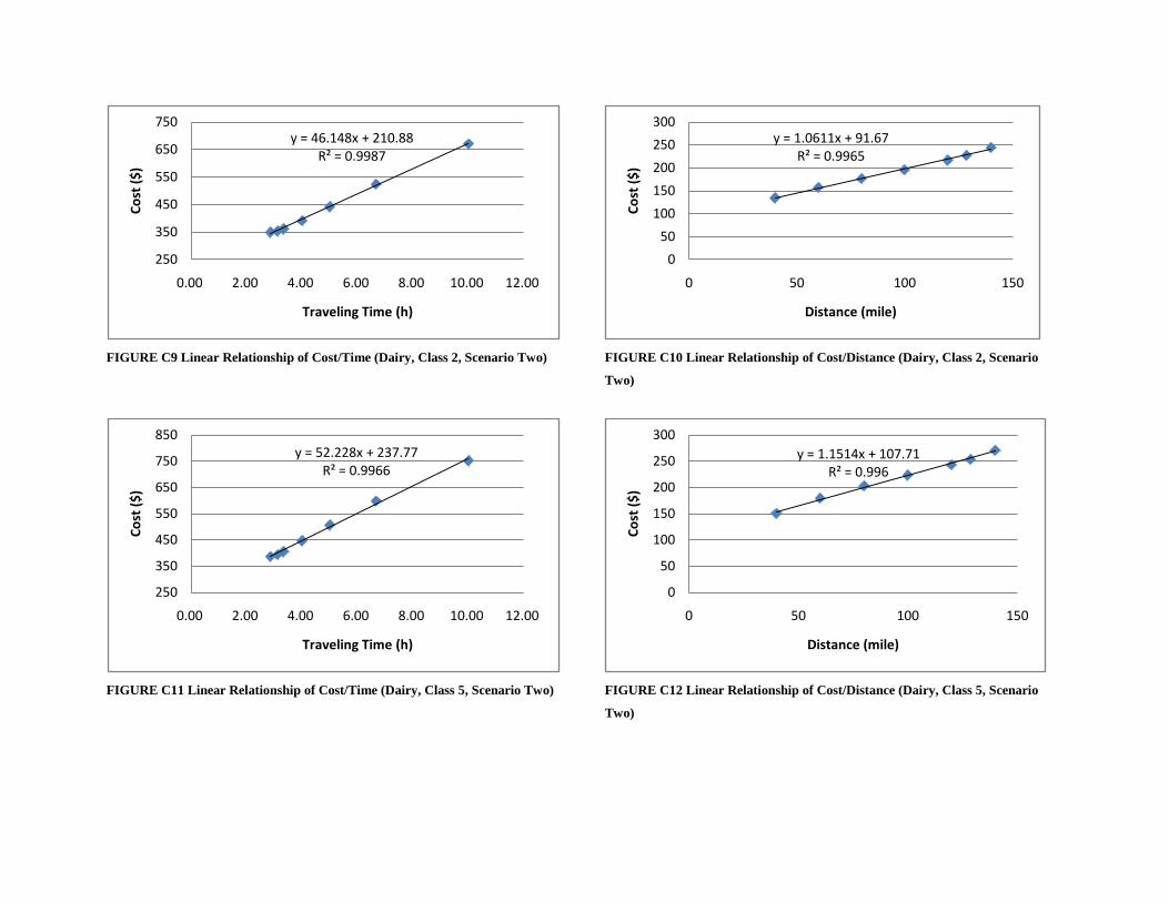
FIGURE C9 Linear Relationship of Cost/Time (Dairy, Class 2, Scenario Two) FIGURE C10 Linear Relationship of Cost/Distance (Dairy, Class 2, Scenario
Two)
FIGURE C11 Linear Relationship of Cost/Time (Dairy, Class 5, Scenario Two) FIGURE C12 Linear Relationship of Cost/Distance (Dairy, Class 5, Scenario
Two)
y = 46.148x + 210.88R² = 0.9987
250
350
450
550
650
750
0.00 2.00 4.00 6.00 8.00 10.00 12.00
Cost
($)
Traveling Time (h)
y = 1.0611x + 91.67R² = 0.9965
0
50
100
150
200
250
300
0 50 100 150
Cost
($)
Distance (mile)
y = 52.228x + 237.77R² = 0.9966
250
350
450
550
650
750
850
0.00 2.00 4.00 6.00 8.00 10.00 12.00
Cost
($)
Traveling Time (h)
y = 1.1514x + 107.71R² = 0.996
0
50
100
150
200
250
300
0 50 100 150Co
st ($
)Distance (mile)

FIGURE C13 Linear Relationship of Cost/Time (Plastics, Class 2, Scenario Two) FIGURE C14 Linear Relationship of Cost/Distance (Plastics, Class 2,
Scenario Two)
FIGURE C15 Linear Relationship of Cost/Time (Plastics, Class 2, Scenario Two) FIGURE C16 Linear Relationship of Cost/Distance (Plastics, Class 2,
Scenario Two)
y = 26.069x + 207.15R² = 0.9941
200
250
300
350
400
450
500
0.00 2.00 4.00 6.00 8.00 10.00 12.00
Cost
($)
Traveling Time (h)
y = 1.0645x + 49.571R² = 0.9945
0
50
100
150
200
250
0 50 100 150
Cost
($)
Distance (mile)
y = 33.747x + 235.98R² = 0.9942
250
300
350
400
450
500
550
600
0.00 2.00 4.00 6.00 8.00 10.00 12.00
Cost
($)
Traveling Time (h)
y = 1.1532x + 69.809R² = 0.9968
0
50
100
150
200
250
0 50 100 150
Cost
($)
Distance (mile)

FIGURE C17 Linear Relationship of Cost/Time (Motor Vehicle Parts, Class 2, FIGURE C18 Linear Relationship of Cost/Distance (Motor Vehicle Parts,
Scenario Two) Class 2, Scenario Two)
FIGURE C19 Linear Relationship of Cost/Time (Motor Vehicle Parts, Class 5, FIGURE C20 Linear Relationship of Cost/Distance (Motor Vehicle Parts,
Scenario Two) Class 5, Scenario Two)
y = 27.486x + 208.87R² = 0.996
0
100
200
300
400
500
600
0.00 2.00 4.00 6.00 8.00 10.00 12.00
Cost
($)
Traveling Time (h)
y = 1.0629x + 53.302R² = 0.9957
0
50
100
150
200
250
0 50 100 150
Cost
($)
Distance (mile)
y = 33.297x + 235.43R² = 0.9947
0
100
200
300
400
500
600
0.00 2.00 4.00 6.00 8.00 10.00 12.00
Cost
($)
Traveling Time (h)
y = 1.1538x + 68.614R² = 0.997
0
50
100
150
200
250
0 50 100 150
Cost
($)
Distance (mile)

APPENDIX D: FIGURES AND TABLES ABOUT PERCENTAGE DISTRIBUTIONS ON THE CUT LINES
FIGURE D1 Percentage Distribution on Cut Line 1 FIGURE D2 Percentage Distribution on Cut Line 2
TABLE D1 Comparison of Percentage Distribution on Cut Line 1 TABLE D2 Comparison of Percentage Distribution on Cut Line 2 Model Output ATR Station
Model Output ATR Station
Run A Run B Run C
Run A Run B Run C
0.5% 8.2% 3.6% 8.8%
0.0% 8.4% 3.2% 10.4% 62.8% 1.4% 41.6% 62.2%
61.2% 1.5% 46.2% 60.7%
36.8% 90.4% 54.8% 29.0%
38.7% 90.1% 50.6% 28.9%

FIGURE D3 Percentage Distribution on Cut Line3 FIGURE D4 Percentage Distribution on Cut Line 4 TABLE D3 Comparison of Percentage Distribution on Cut Line 3 TABLE D4 Comparison of Percentage Distribution on Cut Line 4
Model Output ATR Station
Model Output ATR Station Run A Run B Run C
Run A Run B Run C
21.8% 3.7% 12.4% 26.4%
0.2% 0.1% 0.0% 11.7% 42.3% 95.0% 65.1% 43.5%
95.8% 0.8% 65.6% 74.8%
35.9% 1.3% 22.5% 30.1%
4.0% 99.2% 34.4% 13.5%
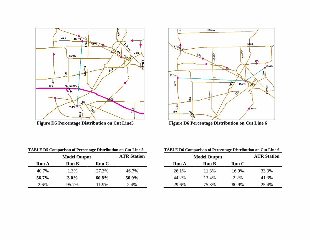
Figure D5 Percentage Distribution on Cut Line5 Figure D6 Percentage Distribution on Cut Line 6
TABLE D5 Comparison of Percentage Distribution on Cut Line 5 TABLE D6 Comparison of Percentage Distribution on Cut Line 6
Model Output ATR Station
Model Output ATR Station Run A Run B Run C
Run A Run B Run C
40.7% 1.3% 27.3% 46.7%
26.1% 11.3% 16.9% 33.3% 56.7% 3.0% 60.8% 50.9%
44.2% 13.4% 2.2% 41.3%
2.6% 95.7% 11.9% 2.4%
29.6% 75.3% 80.9% 25.4%
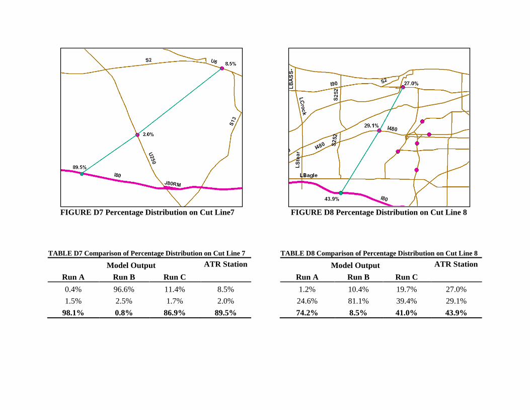
FIGURE D7 Percentage Distribution on Cut Line7 FIGURE D8 Percentage Distribution on Cut Line 8
TABLE D7 Comparison of Percentage Distribution on Cut Line 7 TABLE D8 Comparison of Percentage Distribution on Cut Line 8
Model Output ATR Station
Model Output ATR Station Run A Run B Run C
Run A Run B Run C
0.4% 96.6% 11.4% 8.5%
1.2% 10.4% 19.7% 27.0% 1.5% 2.5% 1.7% 2.0%
24.6% 81.1% 39.4% 29.1%
98.1% 0.8% 86.9% 89.5%
74.2% 8.5% 41.0% 43.9%
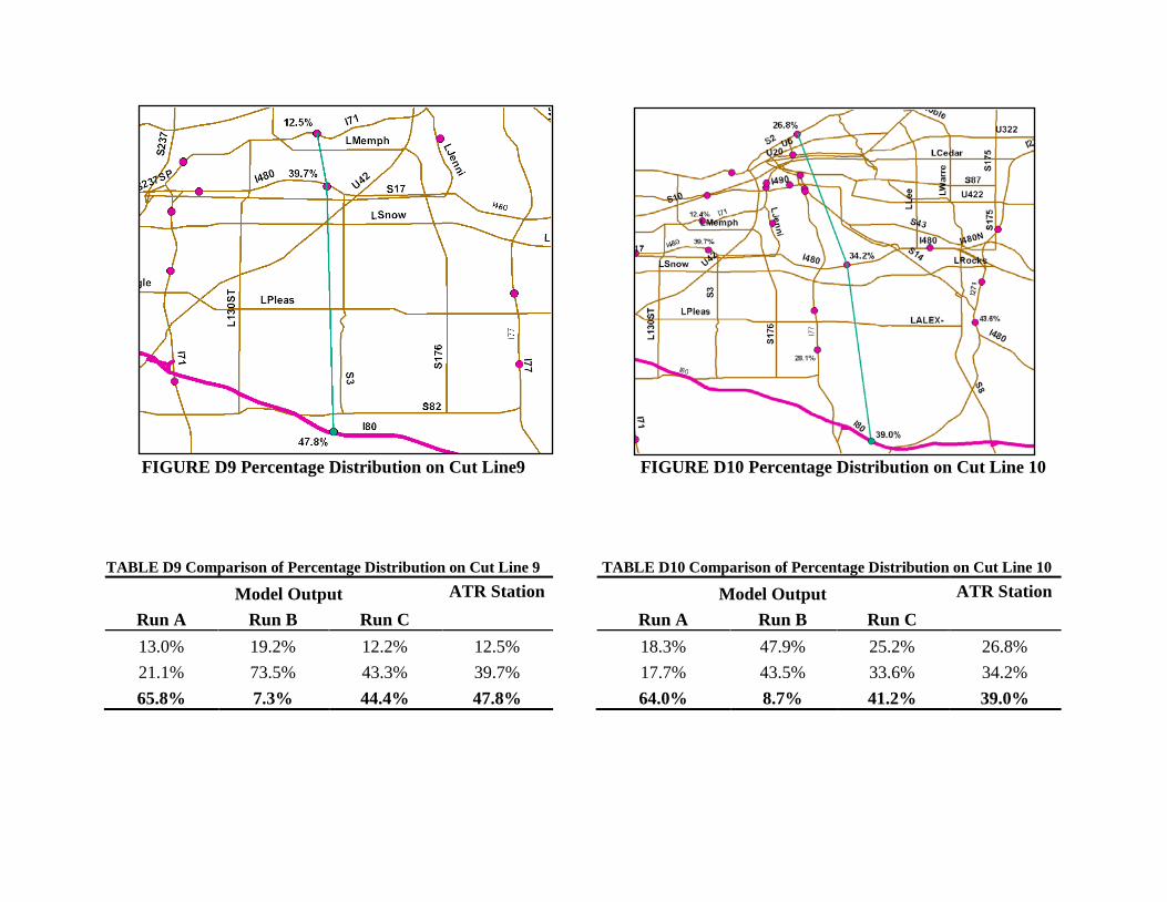
FIGURE D9 Percentage Distribution on Cut Line9 FIGURE D10 Percentage Distribution on Cut Line 10
TABLE D9 Comparison of Percentage Distribution on Cut Line 9 TABLE D10 Comparison of Percentage Distribution on Cut Line 10
Model Output ATR Station
Model Output ATR Station Run A Run B Run C
Run A Run B Run C
13.0% 19.2% 12.2% 12.5%
18.3% 47.9% 25.2% 26.8% 21.1% 73.5% 43.3% 39.7%
17.7% 43.5% 33.6% 34.2%
65.8% 7.3% 44.4% 47.8%
64.0% 8.7% 41.2% 39.0%

FIGURE D11 Percentage Distribution on Cut Line11 FIGURE D12 Percentage Distribution on Cut Line 12
TABLE D11 Comparison of Percentage Distribution on Cut Line 11 TABLE D12 Comparison of Percentage Distribution on Cut Line 12
Model Output ATR Station
Model Output ATR Station Run A Run B Run C
Run A Run B Run C
7.5% 52.4% 24.5% 14.4%
11.3% 12.6% 11.6% 19.1% 14.8% 34.0% 20.4% 29.6%
56.3% 4.5% 30.5% 39.4%
77.7% 13.7% 55.1% 56.0%
32.4% 82.9% 57.8% 41.5%

FIGURE D13 Percentage Distribution on Cut Line13 FIGURE D14 Percentage Distribution on Cut Line 14
TABLE D13 Comparison of Percentage Distribution on Cut Line 13 TABLE D14 Comparison of Percentage Distribution on Cut Line 14
Model Output ATR Station
Model Output ATR Station Run A Run B Run C
Run A Run B Run C
35.8% 38.1% 57.4% 28.3%
71.9% 2.2% 23.9% 50.1% 24.3% 10.4% 8.6% 28.1%
1.8% 56.5% 26.9% 8.4%
39.9% 51.5% 34.0% 43.6%
26.3% 41.3% 49.2% 41.5%
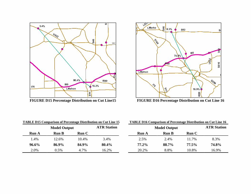
FIGURE D15 Percentage Distribution on Cut Line15 FIGURE D16 Percentage Distribution on Cut Line 16
TABLE D15 Comparison of Percentage Distribution on Cut Line 15 TABLE D16 Comparison of Percentage Distribution on Cut Line 16
Model Output ATR Station
Model Output ATR Station Run A Run B Run C
Run A Run B Run C
1.4% 12.6% 10.4% 3.4%
2.5% 2.4% 11.7% 8.3% 96.6% 86.9% 84.9% 80.4%
77.2% 88.7% 77.5% 74.8%
2.0% 0.5% 4.7% 16.2%
20.2% 8.8% 10.8% 16.9%

FIGURE D17 Percentage Distribution on Cut Line17 FIGURE D18 Percentage Distribution on Cut Line 18
TABLE D17 Comparison of Percentage Distribution on Cut Line 17 TABLE D18 Comparison of Percentage Distribution on Cut Line 18
Model Output ATR Station
Model Output ATR Station Run A Run B Run C
Run A Run B Run C
1.0% 16.1% 12.2% 4.4%
40.1% 39.9% 47.9% 47.2% 91.9% 52.5% 65.0% 80.5%
59.1% 40.0% 45.7% 52.0%
7.1% 31.3% 22.8% 15.1%
0.8% 20.2% 6.3% 0.8%

FIGURE D19 Percentage Distribution on Cut Line19 FIGURE D20 Percentage Distribution on Cut Line 20
TABLE D19 Comparison of Percentage Distribution on Cut Line 19 TABLE D20 Comparison of Percentage Distribution on Cut Line 20
Model Output ATR Station
Model Output ATR Station Run A Run B Run C
Run A Run B Run C
6.0% 4.1% 4.4% 3.3%
52.5% 19.6% 28.3% 50.7% 60.7% 50.7% 53.3% 74.3%
30.4% 19.2% 22.9% 39.3%
33.3% 45.2% 42.3% 22.4%
17.1% 61.2% 48.7% 10.1%