Assessing the ecological impacts of dams on …maps.tnc.org/seacap/assets/SEACAP_Report.pdf ·...
99
Assessing the ecological impacts of dams on Southeastern rivers
-
Upload
dinhnguyet -
Category
Documents
-
view
216 -
download
0
Transcript of Assessing the ecological impacts of dams on …maps.tnc.org/seacap/assets/SEACAP_Report.pdf ·...

Assessing the ecological impacts of dams on Southeastern rivers

1
Corresponding author: December 31, 2014 Erik Martin The Nature Conservancy Eastern Conservation Team 14 Maine Street, Suite 401 Brunswick, ME 04011 [email protected]
Please cite as:
Martin, E. H, Hoenke, K., Granstaff, E., Barnett, A., Kauffman, J., Robinson, S. and
Apse, C.D. 2014. SEACAP: Southeast Aquatic Connectivity Assessment Project:
Assessing the ecological impact of dams on Southeastern rivers. The Nature
Conservancy, Eastern Division Conservation Science , Southeast Aquatic Resources
Partnership. http://www.maps.tnc.org/seacap

2
Funding for this project was generously provided by the South Atlantic Landscape Conservation Cooperative (SALCC).
This project would not have been possible without substantial contributions from the SEACAP Workgroup. Over the two year course of the project, Workgroup members met on a regular basis, provided data, reviewed intermediate datasets and draft results, and provided valuable insight and opinions at key decision points. In particular, we would like to thank (in alphabetical order) Mark Cantrell, Will Duncan, Duncan Elkins, Kathleen Freeman, Paul Freeman, Sara Gottlieb, Chris Goudreau, Will Graf, Chad Holbrook, Ted Hoehn, Jeff Kipp, Wilson Laney, Erin McCombs, Rua Mordecai, Lisa Moss, Robert Newton, Bill Post, Fritz Rhode, Kristina Serbesoff-King, Tyler Stubbs, Alan Weaver, Mike Wicker, Daniel Wieferich and Bennett Wynne….for their involvement on and off Workgroup calls to field in-between-call questions, editing data, and promoting this project to their agencies and other scientists. A complete list of Workgroup participants is included as Appendix I.
Likewise, this project would not have been possible without the previous projects it built upon and the people who spearheaded them. This includes Arlene Olivero Sheldon and Mark Anderson’s work on the Northeast Aquatic Habitat Classification System, the Chesapeake Fish Passage Prioritization Project and the Northeast Aquatic Connectivity project and their respective Workgroups.
Finally, we would like to thank Jeff Zurakowski and Ty Gutherie on The Nature Conservancy’s Spatial Data Infrastructure team for their behind-the-scenes support of the SEACAP web map and custom analysis tool and Susan Hortenstine for her guidance and leadership on project administration.
3
Acknowledgements ..................................................................................................................................... 2
List of Figures ............................................................................................................................................... 5
List of Tables ................................................................................................................................................ 6
1 Background, Approach, and Outcomes .............................................................................................. 7
1.1 Background .................................................................................................................................. 7
1.2 Approach ...................................................................................................................................... 8
1.2.1 Workgroup ............................................................................................................................ 8
1.2.2 Project Extent ........................................................................................................................ 9
2 Data Collection and Preprocessing ..................................................................................................... 9
2.1 Definitions..................................................................................................................................... 9
2.1.1 Functional River Networks ................................................................................................... 9
2.1.2 Watersheds ......................................................................................................................... 10
2.1.3 Stream size class ................................................................................................................ 10
2.2 Hydrography ............................................................................................................................... 11
2.3 Database of Dams ...................................................................................................................... 13
2.3.1 Compilation of Existing Dam Databases ........................................................................... 13
2.3.2 Estimated Dams ................................................................................................................. 14
2.3.3 Final Database .................................................................................................................... 16
2.4 Diadromous Fish Habitat ........................................................................................................... 16
2.5 Resident Fish Data ..................................................................................................................... 17
2.5.1 Species Richness and Rare Species ................................................................................. 17
2.5.2 Species Specific Ranges .................................................................................................... 18
2.6 Waterfalls .................................................................................................................................... 19
3 Analysis Methods ............................................................................................................................... 19
3.1 Metric Calculation ...................................................................................................................... 19
3.1.1 Derived Metrics .................................................................................................................. 21
3.2 Metric Weighting ........................................................................................................................ 22
3.3 Prioritization ................................................................................................................................ 23
4 Results, Uses, & Caveats .................................................................................................................... 25
4.1 Results ........................................................................................................................................ 25
4
4.1.1 Diadromous Fish Scenario ................................................................................................. 25
4.1.2 Resident Fish Scenario ....................................................................................................... 26
4.2 Result Uses ................................................................................................................................. 26
4.3 Data Limitations & Caveats ....................................................................................................... 28
5 Web Map & Custom Analysis Tool .................................................................................................... 30
5.1 Web Map .................................................................................................................................... 31
5.1.1 Project Data ........................................................................................................................ 32
5.1.2 Widgets ............................................................................................................................... 32
5.2 Custom Dam Prioritization Tool ................................................................................................. 37
5.2.1 Applying Custom Weights & Order ................................................................................... 38
5.2.2 Filtering Input Dams ........................................................................................................... 39
5.2.3 Generating Summary Statistics ......................................................................................... 41
5.2.4 Dam Removal Scenarios .................................................................................................... 42
5.2.5 Viewing and Exporting Results .......................................................................................... 45
6 References .......................................................................................................................................... 51
7 Appendix I: SEACAP Workgroup ....................................................................................................... 53
8 Appendix II: Input Datasets ............................................................................................................... 55
9 Appendix III: Resident Fish Species List ........................................................................................... 58
10 Appendix IV: Methodology for Identifying Duplicate Dams ........................................................ 67
11 Appendix V: Glossary and Metric Definitions ............................................................................... 70

5
Figure 1-1: Lassiter Mill Dam on the Uwharrie River in North Carolina was removed in 2013. ............. 7
Figure 1-2: SEACAP Study Area .................................................................................................................. 8
Figure 2-1: Conceptual illustration of functional river networks ............................................................... 9
Figure 2-2: Watershed definitions. ............................................................................................................ 10
Figure 2-3: Size class definitions and map of rivers by size class in the SEACAP study area ............... 11
Figure 2-4: Braided segments highlighted in blue were removed to generate a dendritic network. .... 12
Figure 2-5: Illustration of snapping a dam to the river network .............................................................. 13
Figure 2-6: Cleaning estimated dam data. ................................................................................................ 16
Figure 2-7: Final project data for American shad. .................................................................................... 17
Figure 3-1: A hypothetical example ranking four dams based on two metrics. ..................................... 24
Figure 4-1: Workgroup-consensus Diadromous Fish Scenario results .................................................. 25
Figure 4-2: Workgroup-consensus Resident Fish Scenario results, stratified by subregion ................. 26
Figure 4-3: Steeles Mill Dam on Hitchcock Creek in North Carolina during and after removal .......... 27
Figure 5-1: Conceptual architecture of web map & custom prioritization tool ...................................... 30
Figure 5-2: Web map welcome screen. .................................................................................................. 31
Figure 5-3: Basic features of the web map ............................................................................................... 32
Figure 5-4: Widgets in the Widget Tray .................................................................................................... 33
Figure 5-5: Search widget- find a dam by name. ..................................................................................... 34
Figure 5-6: The Draw widget ..................................................................................................................... 34
Figure 5-7: The Layers widget ................................................................................................................... 35
Figure 5-8: Extract & Download Data widget ........................................................................................... 36
Figure 5-9: The additional Map Layers widget ......................................................................................... 36
Figure 5-10: Custom Dam Prioritization Tool layout ................................................................................ 38
Figure 5-11: Changing the sort order for a metric ................................................................................... 39
Figure 5-12: The Tool with the option to filter input dams highlighted .................................................. 40
Figure 5-13: Building a filter ...................................................................................................................... 40
Figure 5-14: Adding a second filter using the Filter Builder .................................................................... 41
Figure 5-15: Final filter applied from the Filter Builder ............................................................................ 41
Figure 5-16: Selecting the option to run summary statistics on custom prioritization results .............. 42
Figure 5-17: Selecting the option to model dams for removal ................................................................ 43
Figure 5-18: Dams ready to be selected for modeled removal ............................................................... 44
Figure 5-19: A set of dams to be modeled as removed ........................................................................... 45
Figure 5-20: The "Status" state of the Tool displaying updates on a current analysis. .......................... 46
Figure 5-21: The “Results” state ................................................................................................................ 47
Figure 5-22: Select a record in the Results to zoom to a corresponding feature ................................... 48
Figure 5-23: Sorting on a column in the results and buttons to work with the results. ......................... 49
Figure 5-24: Summary statistics of custom scenario results ................................................................... 50
6
Table 3-1: Natural waterbodies that were removed from the NHDPlus v2 waterbodies dataset if they
were represented as polygons. ................................................................................................................. 15
Table 3-2: Invasive fish species attributed to dams based on occurrences within HUC8 watersheds . 18
Table 4-1: Metrics calculated for each dam in the study ........................................................................ 20
Table 4-2: Workgroup-Consensus metric weights for the Diadromous Fish Scenario .......................... 22
Table 4-3: Workgroup-Consensus metric weights for the Resident Fish Scenario. ............................... 23

7
1.1 Background The rivers and streams of the Southeastern United States are extremely diverse, containing numerous
threatened and endangered species. In fact, southeastern rivers contain more at-risk freshwater fish
and invertebrates than any other region of the country (Master et al. 1998).
The anthropogenic fragmentation of river habitats through dams and poorly designed culverts is one of
the primary threats to aquatic species in the United States (Collier et al. 1997, Graf 1999). The impact of
fragmentation on aquatic species generally involves loss of access to quality habitat for one or more life
stages of a species. For example, dams and impassable culverts limit the ability of anadromous fish
species to reach preferred spawning habitats and prevent brook trout populations from reaching
thermal refuges.
Some dams provide valuable services to society including low or zero-emission hydro power, flood
control, and irrigation. Many more dams, however, no longer provide the services for which they were
designed (e.g. old mill dams)
or are inefficient due to age
or design. However, these
dams still create barriers to
aquatic organism passage.
In addition, fish ladders
have long been used to
provide fish passage in
situations where dam
removal is not a feasible
option. In many cases,
these connectivity
restoration projects have
yielded ecological benefits
such as increased
anadromous fish runs,
improved habitat quality
for resident fish species,
and expanded mussel
populations. These projects have been spearheaded by state agencies, federal agencies, municipalities,
NGOs, and private corporations – often working in partnership. Notably, essentially all projects have
had state resource agency involvement. The majority of the funding for these projects has come from
the federal government (e.g. NOAA, USFWS), but funding has also come from state and private sources.
All funding sources have been impacted by recent fiscal instability and federal funding for connectivity
Figure 1-1: Lassiter Mill Dam on the Uwharrie River in North Carolina was removed in
2013.

8
restoration is subject to significant budget tightening and increased accountability for ecological
outcomes.
To many working in the field of aquatic resource management it is apparent that given likely future
constraints on availability of funds and staffing, it will be critical to be more strategic about investments
in connectivity restoration projects. One approach to strategic investment is to assess the likely
ecological “return on investment” associated with connectivity restoration.
The Chesapeake Fish Passage Prioritization Project (Martin and Apse 2013) assessed dams in the
Chesapeake Bay Watershed based on their potential to provide ecological benefits for one or more
targets (e.g. anadromous fish species or resident fish species) if removed or bypassed. Funded by the
South Atlantic Landscape Conservation Cooperative (SALCC), the Southeast Aquatic Connectivity
Assessment Project (SEACAP) grew out of and builds on the conceptual framework of the Chesapeake
Fish Passage Prioritization Project and the Northeast Aquatic Connectivity Project (Martin and Apse
2011). The sections that follow detail the data, methods, results, and tools developed for SEACAP.
1.2 Approach
1.2.1 Workgroup
SEACAP was structured around a project workgroup, the SEACAP Workgroup, composed of members
from federal and state agencies, NGOs, and academia. A full list of Workgroup participants can be found
in Appendix I. Convening via both regular online meetings as well as in-person meetings, the Workgroup
was involved in several key aspects of the project including data acquisition and review, key decision
making, and review of draft results. This collaborative workgroup approach built upon TNC’s successful
experience working with a state agency team to complete the Chesapeake Fish Passage Prioritization
and the Northeast Aquatic Connectivity projects. In addition to providing input throughout the project,
the Workgroup members form a core user base, active
in aquatic connectivity restoration and with a direct and
vested interest in the results.
Central among the key decisions made by the
Workgroup was to define the objectives of the
prioritization. That is, 1) for what benefit are we
prioritizing? and 2) what aspects of a dam or its location
would make its removal or mitigation more likely to
achieve the objective? This process of selecting targets
and the metrics that would be used to evaluate the
dams was both a collaborative and subjective process.
The Workgroup selected two targets: diadromous fish
and resident fish. Different metrics were used to create
two separate prioritization scenarios for these two
targets resulting in two prioritized lists of dams.
Figure 1-2: SEACAP Study Area

9
1.2.2 Project Extent
The study area, which consists of HUC 4 watersheds draining the SALCC region, covers 250,000 square
miles, has over 350,000 miles of mapped rivers and streams, tens of thousands of dams, and hundreds
of thousands of culverts.
Spatial data for the project were gathered from multiple data sources and processed in a Geographic
Information System (GIS) to generate descriptive metrics for each dam. The core datasets included river
hydrography, dams, diadromous fish habitat, resident fish species occurrences, and natural waterfalls.
Additional datasets were used as needed to generate metrics of interest to the Workgroup. These
datasets include land cover and impervious surface data, roads, rare fish, mussel, and crayfish
watersheds, fish species richness, and invasive species occurrences. A complete list of data used in the
project can be found in Appendix II. A further description of the core datasets follows.
2.1 Definitions Several terms are used throughout the discussion of data and metrics. The sections below detail some
important terms for understanding the data and how metrics were calculated.
2.1.1 Functional River Networks
A dam’s functional river network, also referred to as its connected river network or simply its network, is
defined by those stream reaches that are accessible to a hypothetical fish within that network. A given
target dam’s functional river network is bounded by other dams, headwaters, or the river mouth, as is
illustrated in Figure 2-1. A dam’s total functional river network is simply the combination of its
upstream and downstream functional river networks. The total functional network represents the total
distance a fish could theoretically swim within the network if that particular dam was removed.
Figure 2-1: Conceptual illustration of functional river networks
Target Dam
Other
barriers Upstream
Functional Network
Downstream
Functional Network
Target Dam
Other
barriers Total Functional
Network

10
2.1.2 Watersheds
For any given dam, metrics involving three different watershed scales are used in the analysis. The
contributing watershed, or total upstream watershed, is defined by the total upstream drainage area
above the target dam. Several metrics are also calculated within the watershed of a target dam’s
upstream and downstream functional river networks. These local watersheds are bounded by the
watersheds for the next upstream and downstream functional river networks, as illustrated in Figure
2-2.
Figure 2-2: The contributing watershed is defined by the total drainage upstream of a target dam. The upstream and
downstream functional river network local watersheds are bounded by the watershed for the next dams up and down
stream.
2.1.3 Stream size class
Stream size is a critical factor for determining aquatic biological assemblages (Olivero and Anderson
2008; Vannote et al. 1980; Mathews 1998). In this analysis, river size classes, based on the catchment
drainage size thresholds developed for the Northeast Aquatic Habitat Classification System (Olivero and
Anderson 2008), were calculated for each segment of the project hydrography and in turn assigned to
each dam (Figure 2-3). Size classes were used in several ways throughout the analysis including as a
proxy for habitat diversity and to define fish habitat (e.g. American shad use size classes ≥Size 2).

11
Figure 2-3: Size class definitions and map of rivers by size class in the SEACAP study area
1a) Headwaters (<3.861 mi2) 1b) Creeks (>= 3.861<38.61 mi2) 2) Small River (>=38.61<200 mi2) 3a) Medium Tributary Rivers (>=200<1000 mi2) 3b) Medium Mainstem Rivers (>=1000<3861 mi2) 4) Large Rivers (>=3861 < 9653 mi2) 5) Great Rivers (>=9653 mi2) (Defining measure = upstream drainage area)
2.2 Hydrography In order for dams to be included in the analysis, they had to fall on the mapped river network, or
hydrography, that was used in the project: a modified version of the Medium Resolution National
Hydrography Dataset Plus, Version 2 (NHDPlus v2) (Horizon Systems 2012). This hydrography was
originally digitized by the United States Geological Survey primarily from 1:100,000 scale topographic

12
maps. Substantial additions and improvements were applied to the USGS NHD data by Horizon Systems
Corporation to create the NHDPlus v2.
To be used in this analysis, the hydrography was processed to create a dendritic network, or dendrite,
defined as a single-flowline network with no braids or other downstream bifurcation (Figure 2-4).
Attributes in the medium-resolution NHDPlusV2 were queried to identify the mainstem of a river from a
braided section. (NHDFlowline.FLOWDIR = 'With Digitized' AND NHDPlusFlowlineVAA.Divergence in
(0,1) AND NHDPlusFlowlineVAA.StreamCalc <>0). Additional information on the NHDPlus v2 and these
attributes can be found in the NHDPlus v2 User Guide (Horizon Systems 2012).
Figure 2-4: Braided segments highlighted in blue were removed to generate a dendritic network.
The result of this process was a single-flowline dendrite, based on the current Medium Resolution NHD,
for the project area. This dendrite (hereafter referred to as the “project hydrography”) was then further
processed using the ArcGIS Geometric Network toolset in ArcGIS 10.1 to establish flow direction for
each segment. Additional processing using ArcGIS Spatial Analyst and custom Python scripts in ArcGIS
was performed to accumulate upstream attributes for each line segment in the project hydrography.
These processes produced values including the total upstream drainage area, percent impervious
surface, and percent forested land cover for each river segment.

13
2.3 Database of Dams
2.3.1 Compilation of Existing Dam Databases
Dam data was obtained from several sources. Federal data sources constitute the backbone of the
SEACAP dataset providing the locations of larger dams on the project hydrography. These sources
include the US Army Corps of Engineer’s National Inventory of Dams (NID), the USGS Geographic Names
Information System (GNIS) database, the High Resolution NHD Dam Events dataset, and the National
Anthropogenic Barrier Dataset (NABD), which includes dams from the 2009 NID dataset that were
manually aligned to the medium resolution NHD flowlines. To locate dams not represented in these
datasets, the SEACAP project team contacted representative Workgroup members from each state in
the project area, as well as representatives from various state agencies, local watershed groups and
non-profit organizations. Additional datasets were provided from a previous barrier assessment
conducted by the University of Georgia (Elkins and Nibbelink 2012), as well as a manually edited
database composed of multiple sources for the State of North Carolina used in the North Carolina
Barrier Prioritization Tool (Hoenke 2014), a smaller barrier assessment that helped inform this project.
Duplicate dams were removed using a series of steps outlined in 10Appendix IV: Methodology for
Identifying Duplicate Dams. In short, duplicates were identified using federal and State IDs; if neither
were present, search distances of 100 meters were used to identify potential duplicates. If a duplicate
was present, the dam with the best geographic location and most complete attributes was retained.
Data preprocessing and review began after all available data were obtained for each state from the
sources listed above. In order to perform network analyses in a GIS, the points representing dams must
be topologically coincident with lines that represent rivers. This was rarely the case in the dam datasets
as they were received from various data sources. To address this problem, dams were “snapped” in a
GIS to spatially align them with the project hydrography (Figure 2-5).
Figure 2-5: Illustration of snapping a dam to the river network
Dams that were obtained from the NABD had previously been snapped to the medium resolution
(1:100,000) NHD and error checked as part of that project’s review process. Thus, it was assumed that
dams obtained from that project were in the correct location. However, dams from this database had
outdated attribute information, as they were from the NID 2009. To remedy this, the spatial location

14
from dams in NABD was used for duplicates that shared the same NID identifier (NIDID) as dams from
the 2013 NID database, but 2013 attribute information was retained. This method was also used for any
dams from state databases sharing the NIDID with NABD dams, however state attribute information was
retained. Similarly, any dams from local sources having few attributes were given attributes from a
statewide dataset when available, or the NID 2013 dataset.
Snapping for non-NABD dams was performed using the Nature Conservancy’s Barrier Analysis Tool
(BAT). Although snapping is a necessary step which must be run prior to performing the subsequent
network analyses, it also can introduce error into the data. For example, if the point in Figure 2-5 is, in
fact, a dam on the main stem of the pictured river, the snapping will correctly position it on the
hydrography. If, however, the point represents an off-stream farm pond next to the main stem, then
snapping will incorrectly move it onto the hydrography. A snapping tolerance, or “search distance” can
be set to help control which points are snapped. The project team selected a 100 meter snapping
tolerance and developed a review process to error check the results.
The review process for snapped dams involved comparing the snapping distance as well as the
“REACHCODE” attribute, which persists between different versions of the NHD. Dams which snapped to
the project hydrography within the 100m snap tolerance and that had matching REACHCODEs were
considered to be in the correct location. Other dam locations were manually reviewed based on a series
of error ‘flag’ priorities and edited if necessary. Dams were further edited by the workgroup using
ArcGIS Online.
2.3.2 Estimated Dams
The dam databases described above are known to underrepresent the actual number of barriers on the
ground in the Southeastern US, particularly smaller reservoirs and impoundments (Ignatius and Jones
2014; Ignatius and Stallins 2011). We developed an approach to estimate these missing impoundments
using the NHDPlus v2 waterbody polygons and stream polylines. Our approach relied on the assumption
that the presence of a lake or pond likely represented an impoundment as there are few naturally
occurring waterbodies in the Southeastern US. We first removed known natural waterbodies
represented in the NHDPlus v2 data (Table 2-1). For the state of Florida, we obtained the Florida Natural
Areas Inventory (FNAI) Cooperative Land Cover, Version 2.1 (Dec. 2013) and removed all NHDPlus v2
waterbody polygons whose centroid occurred in a natural waterbody land cover (e.g., basin swamp,
bottomland forest, floodplain swamp, hydric hammock, etc.). In addition to removing known natural
waterbodies, we delineated a tidal-influence zone within which natural and estuarine waterbodies were
likely to occur. To create this zone, we applied two elevation thresholds to a 30-m Digital Elevation
Model (DEM) derived from a seamless mosaic of the National Elevation Dataset (NED; Gesch 2007;
Gesch et al. 2002). We used a 2 m threshold for the Atlantic Coast and a 1 m limit for the Gulf of Mexico
based on expert opinion and tidal information. Any NHDPlus v2 waterbodies that occurred within this
zone were not used in the estimated dam analysis. After removing known and likely natural
waterbodies, we dissolved the NHDPlus waterbodies by ReachCode to address cases where continuous
lakes were represented as separate but adjacent polygons. All NHDPlus flowlines coded as Artificial
Path, Connector, or CanalDitch were selected and then intersected with the dissolved NHDPlus
15
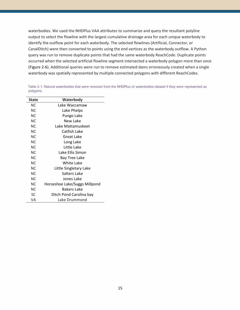
waterbodies. We used the NHDPlus VAA attributes to summarize and query the resultant polyline
output to select the flowline with the largest cumulative drainage area for each unique waterbody to
identify the outflow point for each waterbody. The selected flowlines (Artificial, Connector, or
CanalDitch) were then converted to points using the end vertices as the waterbody outflow. A Python
query was run to remove duplicate points that had the same waterbody ReachCode. Duplicate points
occurred when the selected artificial flowline segment intersected a waterbody polygon more than once
(Figure 2-6). Additional queries were run to remove estimated dams erroneously created when a single
waterbody was spatially represented by multiple connected polygons with different ReachCodes.
Table 2-1: Natural waterbodies that were removed from the NHDPlus v2 waterbodies dataset if they were represented as
polygons.
State Waterbody
NC Lake Waccamaw NC Lake Phelps NC Pungo Lake NC New Lake NC Lake Mattamuskeet NC Catfish Lake NC Great Lake NC Long Lake NC Little Lake NC Lake Ellis Simon NC Bay Tree Lake NC White Lake NC Little Singletary Lake NC Salters Lake NC Jones Lake NC Horseshoe Lake/Suggs Millpond NC Bakers Lake SC Ditch Pond Carolina bay VA Lake Drummond
16
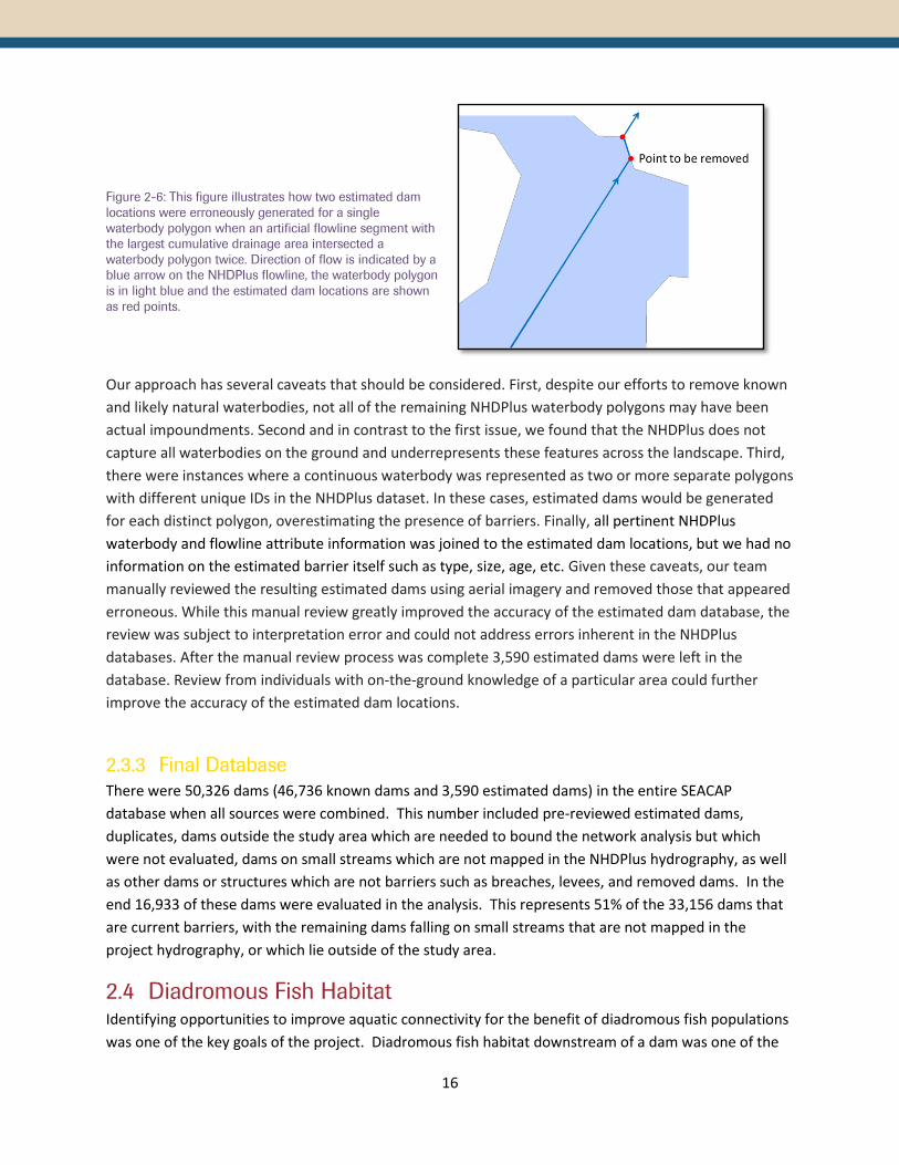
Figure 2-6: This figure illustrates how two estimated dam
locations were erroneously generated for a single
waterbody polygon when an artificial flowline segment with
the largest cumulative drainage area intersected a
waterbody polygon twice. Direction of flow is indicated by a
blue arrow on the NHDPlus flowline, the waterbody polygon
is in light blue and the estimated dam locations are shown
as red points.
Our approach has several caveats that should be considered. First, despite our efforts to remove known
and likely natural waterbodies, not all of the remaining NHDPlus waterbody polygons may have been
actual impoundments. Second and in contrast to the first issue, we found that the NHDPlus does not
capture all waterbodies on the ground and underrepresents these features across the landscape. Third,
there were instances where a continuous waterbody was represented as two or more separate polygons
with different unique IDs in the NHDPlus dataset. In these cases, estimated dams would be generated
for each distinct polygon, overestimating the presence of barriers. Finally, all pertinent NHDPlus
waterbody and flowline attribute information was joined to the estimated dam locations, but we had no
information on the estimated barrier itself such as type, size, age, etc. Given these caveats, our team
manually reviewed the resulting estimated dams using aerial imagery and removed those that appeared
erroneous. While this manual review greatly improved the accuracy of the estimated dam database, the
review was subject to interpretation error and could not address errors inherent in the NHDPlus
databases. After the manual review process was complete 3,590 estimated dams were left in the
database. Review from individuals with on-the-ground knowledge of a particular area could further
improve the accuracy of the estimated dam locations.
2.3.3 Final Database
There were 50,326 dams (46,736 known dams and 3,590 estimated dams) in the entire SEACAP
database when all sources were combined. This number included pre-reviewed estimated dams,
duplicates, dams outside the study area which are needed to bound the network analysis but which
were not evaluated, dams on small streams which are not mapped in the NHDPlus hydrography, as well
as other dams or structures which are not barriers such as breaches, levees, and removed dams. In the
end 16,933 of these dams were evaluated in the analysis. This represents 51% of the 33,156 dams that
are current barriers, with the remaining dams falling on small streams that are not mapped in the
project hydrography, or which lie outside of the study area.
2.4 Diadromous Fish Habitat Identifying opportunities to improve aquatic connectivity for the benefit of diadromous fish populations
was one of the key goals of the project. Diadromous fish habitat downstream of a dam was one of the

17
most important factors chosen by the Workgroup for
the Diadromous Fish Scenario to determine which
dams have the greatest potential for ecological
benefit if removed or mitigated.
Baseline habitat data were collected for American
shad, hickory shad, Alabaman shad, blueback herring,
alewife, striped bass, Atlantic sturgeon, and gulf
sturgeon. These data were collected from the
Atlantic States Marine Fisheries Commission (ASMFC
2004), as well as from the National Fish Habitat
Partnership (NFHAP) database (Esselman et al 2013),
the Multistate Aquatic Resources Information System
(MARIS- http://www.marisdata.org/), and the North
Carolina Museum Collection data
(http://collections.naturalsciences.org/). These data
were extensively reviewed and edited by fisheries
biologists in the spring of 2014 at the Southern
Division American Fisheries Society meeting in
Charleston, South Carolina, as well as through a
series of follow-up online meetings. This review
process incorporated additional fish observance data as well as expert knowledge from biologists.
2.5 Resident Fish Data Resident fish species data were attributed to dams using a suite of species occurrence data available at
the 8-digit HUC watershed (HUC8s). Resident fish species data were assigned to HUC8 watersheds, as
opposed to stream reaches, to help account for sampling inconsistencies and bias. These resident fish
species data were used to calculate a fish species richness metric for use as a weighted metric in custom
analysis scenarios. Additionally, the range of individual fish species can be used to filter dams in a
custom analysis (e.g. only analyze dams that are in a watershed which supports rainbow darter.)
2.5.1 Species Richness and Rare Species
For users wishing to prioritize dams based on the variety of species present in a dam’s watershed, a
suite of optional ecological metrics are available. Two separate fish species richness values were
calculated. The first was based directly on a NatureServe-calculated fish species richness metric which
measures total resident fish species richness for all species in the NatureServe database. A second fish
richness metric was calculated for species of interest identified by the Workgroup using data compiled
from multiple sources (see Section 2.5.2). Freshwater mussel richness was calculated from NatureServe
data in a similar manner, using individual species layers from NatureServe at the HUC8 scale. Finally, the
numbers of rare fish, rare mussel and rare crayfish (G1-G3) in a HUC8 were obtained directly from
NatureServe’s HUC8 data.
Figure 2-7: Final project data for American shad.

18
2.5.2 Species Specific Ranges
In addition to providing the option to use species richness data as weighted metrics in a custom
prioritization, the option is also presented to use a specific species’ HUC8 range to limit the analysis
inputs. Doing so would limit the analysis to only those dams that are in a watershed where that species
is found. For example, an analysis could be performed to prioritize dams based on a user-defined suite
of habitat metrics, but limited geographically to dams in watersheds with documented occurrences of
robust redhorse. This could be useful if there was interest or funding to target passage projects to
benefit a specific species or suite of species.
The species-specific HUC8 range maps were created by compiling three data sources: NatureServe
HUC8-scale data, Multistate Aquatic Resources Information System (MARIS) point occurrence data, and
USGS Biodiversity Information Serving Our Nation (BISON) database point occurrence data. Erring on
the side of inclusion, any HUC8 where a given species was present in any of the three input data sources
was assigned a value of “present” for that species. If none of the three data sources had records for a
given species in a given HUC8, that HUC8 was assigned a value of “Absent.” Each dam inherited the
presence/absence value for each species from the HUC8 it was within. A complete list of the resident
fish species used can be found in Appendix III: Resident Fish Species List.
Similarly to resident species, invasive species data were also made available at the HUC8 scale so that a
user can filter prioritized dams and eliminate dams from the prioritization that may contain invasive
species in the watershed. These data were compiled from the USGS Nonindigenous Aquatic Species
(NAS) database and MARIS. Invasive species included in this dataset were selected by the SEACAP
Workgroup and are presented in Table 2-2.
Table 2-2: Invasive fish species attributed to dams based on occurrences within HUC8 watersheds
Scientific Name Common Name
Channa argus Northern Snakehead
Channa maculata Blotched Snakehead
Channa marulius Bullseye Snakehead
Clarias batrachus Walking Catfish
Cyprinella lutrensis Red Shiner
Dreissena polymorpha Zebra Mussel
Hypophthalmichthys molitrix Silver Carp
Hypophthalmichthys nobilis Bighead Carp
Ictalurus furcatus Blue Catfish
Ictiobus bubalus Smallmouth Buffalo
Ictiobus cyprinellus Bigmouth Buffalo
Micropterus coosae Redeye Bass
Micropterus dolomieu Smallmouth Bass
Micropterus henshalli Alabama Bass
Misgurnus anguillicaudatus Oriental Weatherfish

19
Oncorhynchus mykiss Rainbow Trout
Pylodictis olivaris Flathead Catfish
Salmo trutta Brown Trout
2.6 Waterfalls Waterfalls, like dams, can act as barriers to fish passage. Including them in the analysis was important
due to the impact natural barriers have across a network. For example, a waterfall just upstream of a
dam would drastically affect the length of that dam’s upstream functional network, or the number of
river miles that would be opened by providing passage at that dam. Thus, although waterfalls are
excluded from the project results, they were included in the generation of functional networks.
The primary data source for waterfalls was the USGS Geographic Names Information System (GNIS)
database, which includes named features from 1:100,000 scale topographic maps. Additional waterfalls
that were part of an initial effort of the USGS Aquatic GAP Program to compile a national waterfall
database (Daniel Wieferich, personal communication) were also included. All waterfall data were
merged together and snapped to the project hydrography using the same method previously described
for dams.
The conceptual framework of the Southeast Aquatic Connectivity Assessment Project rests on a suite of
ecologically relevant metrics calculated for every dam in the study area. These metrics are then used to
evaluate the benefit of removing or providing passage at any given dam relative to any other dam. At its
simplest, a single metric could be used to evaluate dams. For example, if one is interested in passage
projects to benefit diadromous fish, the dam’s upstream functional network length, or the number of
river miles that would be opened by that dam’s removal, could be used to prioritize dams. In this case,
the dam with the longest upstream functional network—the dam whose removal would open up the
most river miles—would rank at the top of the list. As multiple metrics are evaluated, weights can be
applied to indicate the relative importance of each metric in a given scenario, as described in further
detail in Section 3.2.
3.1 Metric Calculation A total of 43 metrics were calculated for each dam in the study area using ArcGIS 10.1. Metrics were
organized into five categories for convenience: Connectivity Status, Connectivity Improvement,
Watershed/Local Condition, Ecological, and Size/System Type. Additionally, each metric is sorted in
either ascending order or descending order to indicate whether large values or small values are
desirable in a given scenario. For example, upstream functional network length is sorted descending
because large values are desirable – a passage project on a dam that opens up more river miles is
desired over a passage project which opens up few miles. Conversely, percent impervious surface is
sorted ascending because small values are desirable – a passage project that opens up a watershed that

20
has little or no impervious surface is desired over a dam that opens up a watershed with a high
percentage of impervious surface. Each of the metrics is presented in Table 3-1, and a more complete
description of each metric can be found in Appendix V: Glossary and Metric Definitions.
Table 3-1: Metrics calculated for each dam in the study
Metric Category
Metric Unit Default
Sort Order
Connectivity Status
# Dams Downstream # A
# Dams Upstream # A
Total Upstream River Length m D
Downstream Waterfall Count on Flowpath # A
Downstream Hydropower Dam Count on Flowpath # A
Number of Dams on High Resolution NHD in upstream Drainage Area # A
Upstream Barrier Density #/m A
Downstream Barrier Density #/m A
Density of Small (Unsnapped) Dams in Upstream Functional Network Local Watershed #/m² A
Density of Small (Unsnapped) Dams in Downstream Functional Network Local Watershed
#/m² A
Density of Road & RR / Small Stream Crossings in Upstream Functional Network Local Watershed
#/m² A
Density of Road & RR / Small Stream Crossings in Downstream Functional Network Local Watershed
#/m² A
Connectivity Improvement
Upstream Functional Network Length m D
The total length of upstream and downstream functional network m D
Downstream Functional Network Size m D
Relative Gain m D
Absolute Gain m D
Watershed / Local
Condition
% impervious surface in Upstream Drainage Area % A
% natural landcover in Upstream Drainage Area % D
% forest cover in Upstream Drainage Area % D
% agriculture in Upstream Drainage Area % A
% Impervious Surface in ARA of Upstream Functional Network % A
% Impervious Surface in ARA of Downstream Functional Network % A
% Agriculture in ARA of Upstream Functional Network % A
% Agriculture in ARA of Downstream Functional Network % A
% Natural LC in ARA of Upstream Functional Network % D
% Natural LC in ARA of Downstream Functional Network % D
% Forested LC in ARA of Upstream Functional Network % D
% Forested LC in ARA of Downstream Functional Network % D

21
Metric Category
Metric Unit Default
Sort Order
Dam is Located on Conservation Land Boolean D
NFHAP Risk of Degradation Score # A
Total storage / mean annual flow cfs D
Ecological
# Diadromous Species in DS Network # D
Presence of Diadromous Species in DS Network Boolean D
Resident fish species richness (NatureServe - all resident fish) # D
Resident Fish Species Richness (HUC 8) Calculated Based on Workgroup List # D
Resident Mussel Species Richness (HUC 8) Calculated Based on Workgroup List # D
# of rare (G1-G3) fish HUC8 # D
# of rare (G1-G3) mussel HUC8 # D
# of rare (G1-G3) crayfish HUC8 # D
Size / System Type
Number of new upstream size classes >0.5 miles gained by removal / bypass # D
Total Reconnected # stream sizes (upstream + downstream) >0.5 Mile # D
River Size Class # D
3.1.1 Derived Metrics
3.1.1.1 Active River Area
The Active River Area (ARA) is a spatially explicit framework for modeling rivers and their dynamic interaction with the land through which they flow (Smith et al. 2008). Key features of the ARA include the meander belt, riparian wetlands, floodplains, terraces, material contribution areas. The ARA is different from, but was calibrated to and compared against the FEMA 100‐year floodplain. The SEACAP project used the ARA as a unit within which various landcover metrics, such as forest cover and impervious surface, were summarized. For the SEACAP project area, we delineated the ARA for each of the seven size classes described in Section 2.1.3, using a seamless mosaic of 10m DEM data from the National Elevation Dataset (Gesch 2007; Gesch et al. 2002) as well as stream polylines, waterbody polygons, and stream area polygons from the NHDPlus v2 dataset. We selected and resampled wetflat landforms from a 30m landform model developed for the Southeastern US (Anderson et al. 2014) to identify ARA components that occurred on wetflats and where longer-term storage of water is expected to occur. In addition, we obtained 100-yr floodplain polygons from the FEMA National Flood Hazard Layer (NFHL) in spring 2013 and used this data to inform cost distance threshold selection in the ARA delineation. Any FEMA 100-yr floodplain areas that were not captured by the ARA delineation were gridded at 10m resolution and merged underneath the ARA components in the final product. The final 10m ARA was resampled to 30m for use in the SEACAP metric calculations due to the resolution of other key input datasets (i.e., landcover).

22
The methods used to calculate all metrics was automated and documented via ArcGIS Model Builder
models and custom Python scripts. Contact the authors for more information on the methods used to
calculate metrics.
3.2 Metric Weighting Depending on the objectives of a prioritization scenario some metrics will be of greater importance than
other metrics. Thus, metrics are selected and weighted to develop a scenario for a given objective. For
example, if the objective of a prioritization scenario is to identify dams which would benefit diadromous
fish if passed, upstream functional network length may be of particular interest, while the percent
impervious surface in a dam’s watershed may be of less importance, and the presence of rare crayfish
species may be of no interest. Relative weights, which must sum to 100, can be assigned to each metric
to indicate its importance in a given scenario. Table 3-2 and Table 3-3 list the weights chosen by the
SEACAP Workgroup, through an iterative, consensus-based process for the Diadromous Fish Scenario
and the Resident Fish Scenario respectively.
Metric weights are subjective in nature; there are no hard and fast rules regarding how to properly
select and weight metrics for a given target like diadromous fish. To arrive at the weights presented in
the tables below, the Workgroup went through an iterative process of selecting draft weights based on
their knowledge of the species of interest, then adjusting the weights in response to draft results and
based on participants’ current removal priorities. This process allowed the Workgroup to both
understand the impact of making an adjustment to a given metric weight, and also served to better
calibrate the results to known priorities.
Table 3-2: Workgroup-Consensus metric weights for the Diadromous Fish Scenario
Metric Category
Metric Diadromous
Weight
Connectivity Status
Downstream Dam Count on Flowpath 10
Downstream Hydropower Dam Count on Flowpath 5
Total Upstream River Length 10 Density of Road & Railroad / Small Stream Crossings in Upstream Functional Network Local Watershed 10
Connectivity Improvement
Upstream Functional Network Size 15
The total length of upstream and downstream functional network 5
Watershed / Local Condition
% impervious surface in Upstream Drainage Area 5
% natural landcover in Upstream Drainage Area 5
% Impervious Surface in ARA of Upstream Functional Network 5
Total storage / mean annual flow 5
Ecological # Diadromous Species in DS Network (incl Eel) 5
Presence of Anadromous Species in DS Network 15 Size / System
Type # Upstream Size Classes >0.5mi gained 5

23
Table 3-3: Workgroup-Consensus metric weights for the Resident Fish Scenario.
Metric Category
Metric Resident Weight
Connectivity Status
Density of All Small Dams (Snapped to High Res NHD or not) in Downstream Functional Network Local Watershed 5 Density of Road & Railroad / Small Stream Crossings in Downstream Functional Network Local Watershed 10 Density of All Small Dams (Snapped to High Res NHD or not) in Upstream Functional Network Local Watershed 5 Density of Road & Railroad / Small Stream Crossings in Upstream Functional Network Local Watershed 10
Connectivity Improvement
Absolute Gain 20
Watershed / Local
Condition
% impervious surface in Upstream Drainage Area 10
% forest cover in Upstream Drainage Area 10
% Impervious Surface in ARA of Upstream Functional Network 5
% Impervious Surface in ARA of Downstream Functional Network 5
% Forested LC in ARA of Upstream Functional Network 5
% Forested LC in ARA of Downstream Functional Network 5 Size / System
Type Total Reconnected # stream sizes (upstream + downstream) >0.5 Mile 10
In addition to assigning relative weights for metrics, the universe of dams that are included in an analysis
can be filtered. For example, only dams on small streams can be included in the prioritization if desired.
Filters such as this can be based on geography (e.g. state, watershed) or any attribute (e.g. dam
purpose, presence of a specific diadromous species). Additional details on using filters can be found in
Section 5: Web Map and Custom Analysis Tool.
Of note, the SEACAP Workgroup chose to focus weighted metrics on habitat factors for the resident fish
scenario, reserving biological data for use in the custom analysis tool as weighted metrics (e.g. fish
species richness) or filters (e.g. only prioritizes dams in watersheds where robust redhorse are present).
3.3 Prioritization Once metric values were calculated and relative weights assigned to the metrics of interest, metrics
were combined through a weighted ranking process to develop a prioritized list for each scenario. The
ranking process involves four steps and simple mathematical operations, as illustrated in .

24
Step 1: Raw values are calculated for each metric in GIS
Step 2: Raw values are ranked. For each metric, ranks are determined based on whether large
values are desirable in a scenario (e.g. upstream functional network length) or small values are
desirable (e.g. % impervious surface)
Step 3: Ranked values are converted to a percent scale where the top ranked value is assigned a
score of 100 and the lowest ranked value is assigned a score of 0.
Step 4-5: Multiply the percent rank by the chosen metric weight
o In this hypothetical example, assume upstream functional network length weight = 75
and downstream functional network length weight = 25.
Step 6: Sum the weighted ranks for each metric for each dam
o All metrics which are included in the analysis (weight >0) are summed to give a summed
rank.
Step 7: Rank the summed ranks
o The summed ranks are, in turn, ranked
Raw
Val
ues HUC12 Upstream Functional Network
Length (m) Downstream Functional Network
Length (m)
Dam A 239,541 2,572
1 Dam B 342,654 62,525
Dam C 572,594 6,233
Dam D 125,213 87,425
Ran
ked
Val
ue
s HUC12 Upstream Functional Network Length (rank)
Downstream Functional Network Length (rank)
Dam A 3 4
2 Dam B 2 2
Dam C 1 3
Dam D 4 1
% R
anke
d V
alu
es
HUC12 Upstream Functional Network
Length (% rank) Downstream Functional Network
Length (% rank)
Dam A 33 0
3 Dam B 66 66
Dam C 100 33
Dam D 0 100
Mu
ltip
ly b
y W
eigh
t
HUC12 Upstream Functional Network
Length Downstream Functional Network
Length
Dam A 33 * 0.75 0 * 0.25
4 Dam B 66 * 0.75 66 * 0.25
Dam C 100 * 0.75 33 * 0.25
Dam D 0 * 0.75 100 * 0.25
Wei
ghte
d R
ank
Val
ues
HUC12 Upstream Functional Network
Length (weighted rank) Downstream Functional Network
Length (weighted rank)
Dam A 25 0
5 Dam B 50 16.6
Dam C 75 8.3
Dam D 0 25
Co
mb
ined
Sco
re
HUC12 Combined Score
Dam A 25 6 Dam B 66.6
Dam C 83.3
Dam D 25
Fin
al R
ank HUC12 Final Rank
Dam A 3
7 Dam B 2
Dam C 1
Dam D 3
Figure 3-1:A hypothetical example ranking four dams based on two metrics.
25
The final ranks are then binned into 5% tiers for presentation. This is an important step in
acknowledging that the precision with which metrics can be calculated in a GIS is not necessarily
indicative of on-the-ground differences. For example, a dam which opens up 3.234 miles of river habitat
may not provide greater ecological benefit than a dam which opens up 3.25 miles of habitat.
4.1 Results Results from the project include lists of dams prioritized based on two scenarios agreed upon by the
Workgroup: diadromous fish scenario and resident fish scenario. These consensus-based scenarios were
developed by selecting metrics and applying relative weights (see Section 3.2) for the dams and data
compiled for the project (see Section 2). These results can be viewed and downloaded from
http://maps.tnc.org/seacap.
Of note, dams with existing fish passage facilities are included in the results. Given the variability of fish
passage functionality and the species passed during various flow conditions, as well as the relative lack
of data to describe passage success rates, it was determined that these dams should remain in the
analysis. Even dams with passage facilities are barriers to one degree or another and, if circumstances
are conducive, their removal will benefit aquatic
connectivity.
Although the prioritization produces a sequential
list of dams, the precision with which metrics can
be calculated in a GIS is not necessarily indicative
of ecological differences. Therefore, throughout
this report and on the project web map, results
are binned in Tiers for presentation where each
Tier includes 5% of the dams in the study area.
Thus, 5% of the total dams are in the top Tier,
Tier 1. These dams would provide the greatest
ecological benefit to the given target if removed
or otherwise remediated.
4.1.1 Diadromous Fish Scenario
The first scenario which was defined by the
Workgroup was a scenario to prioritize dams
based on their potential to benefit diadromous
fish species if removed or bypassed. This
scenario was developed using the metric weights presented in Table 3-2, and produced the results
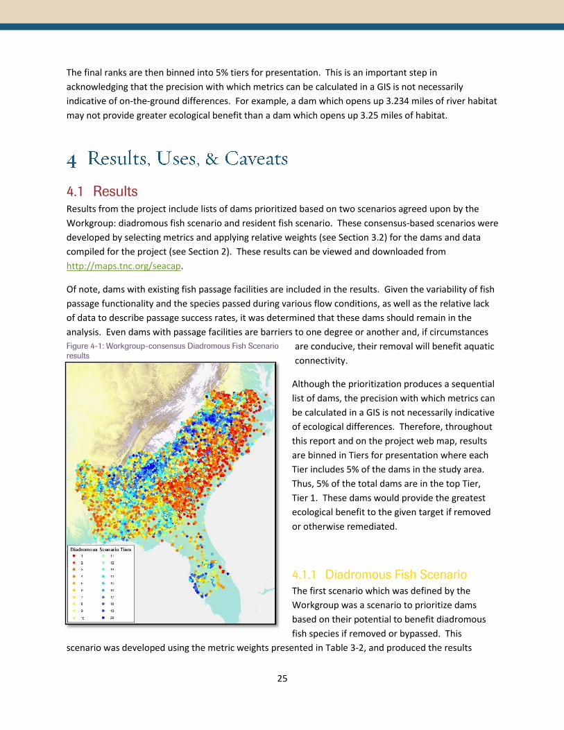
Figure 4-1: Workgroup-consensus Diadromous Fish Scenario
results

26
depicted in Figure 4-1. As one would expect in a scenario designed to benefit diadromous fish, the dams
in the higher tiers, those whose removal would provide the greatest benefit to diadromous fish, tend to
be found closer to the ocean and on the larger mainstem rivers. These include the major rivers in
Southeastern states and many smaller coastal streams. These results directly reflect the metrics chosen
and weights applied to them including anadromous fish presence (weight=15), number of dams
downstream (weight = 10), and upstream functional network size (weight = 15).
4.1.2 Resident Fish Scenario
Using the metrics and metrics weights selected
by the SEACAP Workgroup (in Table 3-3), a
Resident Fish Scenario was developed. This
scenario was intended to reflect priorities for a
set of non-migratory fish species like suckers,
black basses, brook trout, shiners, or darters. As
illustrated in Figure 4-2, these results differ
substantially from the Diadromous Fish Scenario
result. They are driven by absolute gain
(weight=20), total reconnected number of
stream sizes greater than 0.5 miles (weight=10),
and a suite of land cover condition and stream
crossing density metrics.
Unlike the diadromous fish scenario, the
Workgroup chose to stratify the analysis based
on three subregions. The regions, including the
South Atlantic Coastal Region, South Atlantic
Piedmont, and Gulf drainages, were defined by
the SEACAP Core team and the Workgroup to
reflect regional patterns of resident fish
distribution and diverse assemblages of fish found in the subregions. The prioritization analysis was run
separately in each of the three subregions, and then the results were stitched back together for the
entire project area. Figure 4-2 depicts the results of the resident fish scenario, including the three
stratification regions.
4.2 Result Uses The Southeast Aquatic Connectivity Assessment Project can be used in several different ways to inform
and support on-the-ground efforts to restore aquatic connectivity.
Figure 4-2: Workgroup-consensus Resident Fish Scenario
results, stratified by subregion
27
Project Selection: A primary use is to help managers direct their limited resources to projects
that can have the greatest benefit; to help them move away from a purely opportunistic
approach to more of an ecological benefits approach (recognizing that opportunity among other
non-ecological factors does and will continue to play an important role in project selection).
Directing resources where they can have the greatest impact is increasingly important as federal
and state budgets shrink in our current fiscal environment.
Improve Understanding of
Current Conditions: Project results
from the previous studies (Chesapeake
Fish Passage Prioritization) have been
used to help direct managers to
investigate previously unvisited dams
to assess them for potential passage
projects (Jim Thompson, MD DNR,
personal communication March 13,
2013). In some cases this may reveal
errors in the source data while in other
cases it may direct attention to
potential projects that had previously
not been considered.
Database of Ecologically
Relevant Metrics: Prioritization aside,
the results form a database of dams
with 43 ecologically relevant metrics.
These metrics can be used to
investigate many aspects of aquatic
connectivity on a dam-by-dam basis or
other off-shoot analyses. For instance,
a project manager with an
opportunistic passage project can
benefit from easy access to metric
data, quickly identifying the dam’s
restoration potential if removed or
bypassed. Metric data including length
of connected network, species present
downstream, and land cover
characteristics are some examples. In addition, as described further in Section 5, custom
analyses can be performed as if one or more dams have been removed. Metric values and the
prioritization are recalculated as if that dam had been removed, thus allowing managers to
assess the potential impacts of proposed projects.
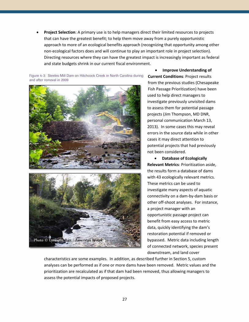
Figure 4-3: Steeles Mill Dam on Hitchcock Creek in North Carolina during
and after removal in 2009
Photo © Peter Raabe / American Rivers
Photo © Lynnette Batt / American Rivers
28
Funding: The prioritized results can be used both by managers seeking funding for a potential
project and by funders looking for information to inform or support a funding allocation
decision.
Watershed Analysis: Subwatersheds can be assessed based on the project results. Summary
statistics can be generated via the custom analysis tool to provide an understanding of potential
opportunities for passage projects in watersheds across the region.
Communication: Results can be used to communicate the value of a given project to the local
community, elected officials, or others with an interest in aquatic connectivity issues.
4.3 Data Limitations & Caveats As with any modeled analysis, there are several
caveats and limitations that are important to bear
in mind when considering the results and data
produced by this project and the custom analysis
tool. First and foremost among them, the results
are not intended to be a “hit list” of dams for
removal. There are many cases where the
benefits provided by a given dam outweigh the
ecological benefits of removing it, although other
passage projects can be considered when removal
is not the best option.
Next, this project is based on data from many
different sources (see Section 2). Each of these
sources brings its own inherent error to the
analysis. For example, the river hydrography, as
represented in the NHD, does not perfectly
represent flowing rivers on the ground. Any
inaccuracies in the source data will be reflected in the metrics calculated using that data. For example, if
a river segment is missing from NHD, the upstream functional river length for the dam below the missing
segment will be too short.
Similarly, the prioritization is sensitive to inaccuracies in the dam database. If a dam is erroneously
included in the database, the error ripples beyond the dam itself since its presence will impact the
metrics for surrounding dams. For example, the calculated upstream functional network of the next
dam downstream will be too short, the downstream functional network of upstream dams will be too
short, the count of downstream dams for all dams upstream of the error will be too high, and so on.
Although the SEACAP project team and Workgroup put substantial effort into compiling and revising the
dam data using desktop GIS techniques, it should be expected that some errors remain. Thus, it is
particularly important that results be examined on an individual basis using the best available local-scale
data and on-the-ground knowledge before any actions are taken.

29
Additionally, this project, by design, only considers ecological factors. It does not include any social,
economic, or feasibility factors, largely due to the fact that this information is difficult or impossible to
capture through regionally-available GIS data. These factors could be layered onto the project results
through a subsequent site-scale analysis, as has been done in Connecticut using results from the
Northeast Aquatic Connectivity project (Steve Gephard, CT Department of Energy & Environmental
Protection, personal communication).
Results produced for this project are intended to be screening-level information that can help inform on-
the-ground decision making, using the best available regional data. They are not a replacement for site-
specific knowledge and field work.
Finally, it is important to note that any aquatic connectivity project will have ecological benefits. If an
opportunity arises it should not be rejected solely on the grounds that it does not rank in one of the
upper tiers of this project. Ultimately, whether the benefits provided by a given passage project justify
the costs is a decision that rests with managers using all of the best information at their disposal. We
hope that this project will be a useful and important tool in the aquatic connectivity toolkit, not the only
one.
30
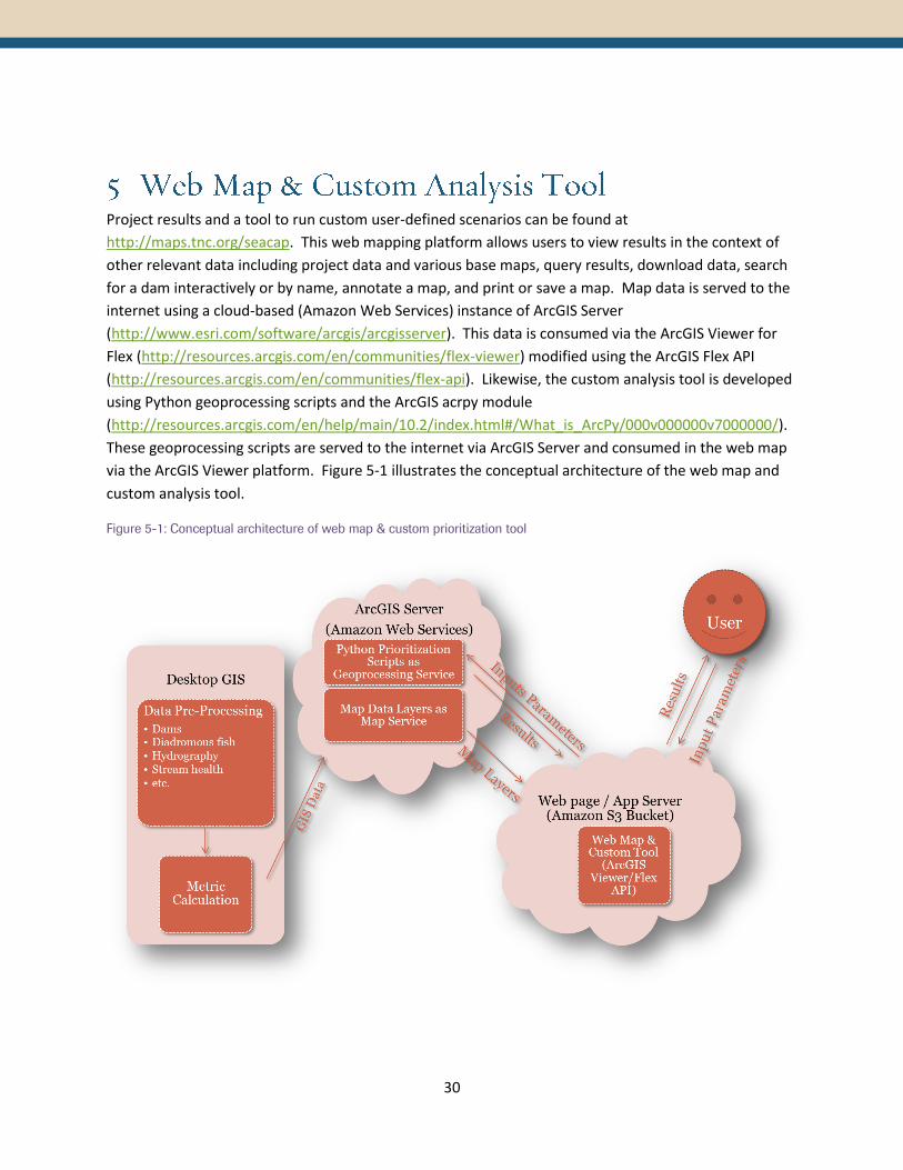
Project results and a tool to run custom user-defined scenarios can be found at
http://maps.tnc.org/seacap. This web mapping platform allows users to view results in the context of
other relevant data including project data and various base maps, query results, download data, search
for a dam interactively or by name, annotate a map, and print or save a map. Map data is served to the
internet using a cloud-based (Amazon Web Services) instance of ArcGIS Server
(http://www.esri.com/software/arcgis/arcgisserver). This data is consumed via the ArcGIS Viewer for
Flex (http://resources.arcgis.com/en/communities/flex-viewer) modified using the ArcGIS Flex API
(http://resources.arcgis.com/en/communities/flex-api). Likewise, the custom analysis tool is developed
using Python geoprocessing scripts and the ArcGIS acrpy module
(http://resources.arcgis.com/en/help/main/10.2/index.html#/What_is_ArcPy/000v000000v7000000/).
These geoprocessing scripts are served to the internet via ArcGIS Server and consumed in the web map
via the ArcGIS Viewer platform. Figure 5-1 illustrates the conceptual architecture of the web map and
custom analysis tool.
Figure 5-1: Conceptual architecture of web map & custom prioritization tool

31
5.1 Web Map Upon first entering the map, a welcome screen pops up with important information about the project,
links to additional information, and use limitations. Three buttons at the bottom of the welcome screen
allows users to enter the map by accepting the use constraints (“Accept”), “Contact” the authors via
email, and link to The Nature Conservancy’s website (“TNC”).
Figure 5-2: Web map welcome screen. Click on "Accept" to agree to the use constraints and enter the map.
By default, the map is loaded with the Workgroup-consensus Diadromous Fish Scenario results
displayed. Clicking on a dam point brings up attribute information including values for all of the metrics
that were used in the diadromous fish scenario. The basic features of the web map are noted in Figure
5-3. At the top of the map window is a tray of “Widgets.” Each widget opens a new window that
contains some discrete functionality for use within the map. Widgets can be minimized, closed,
expanded and dragged. Details about the different map widgets can be found in Section 5.1.2.
32
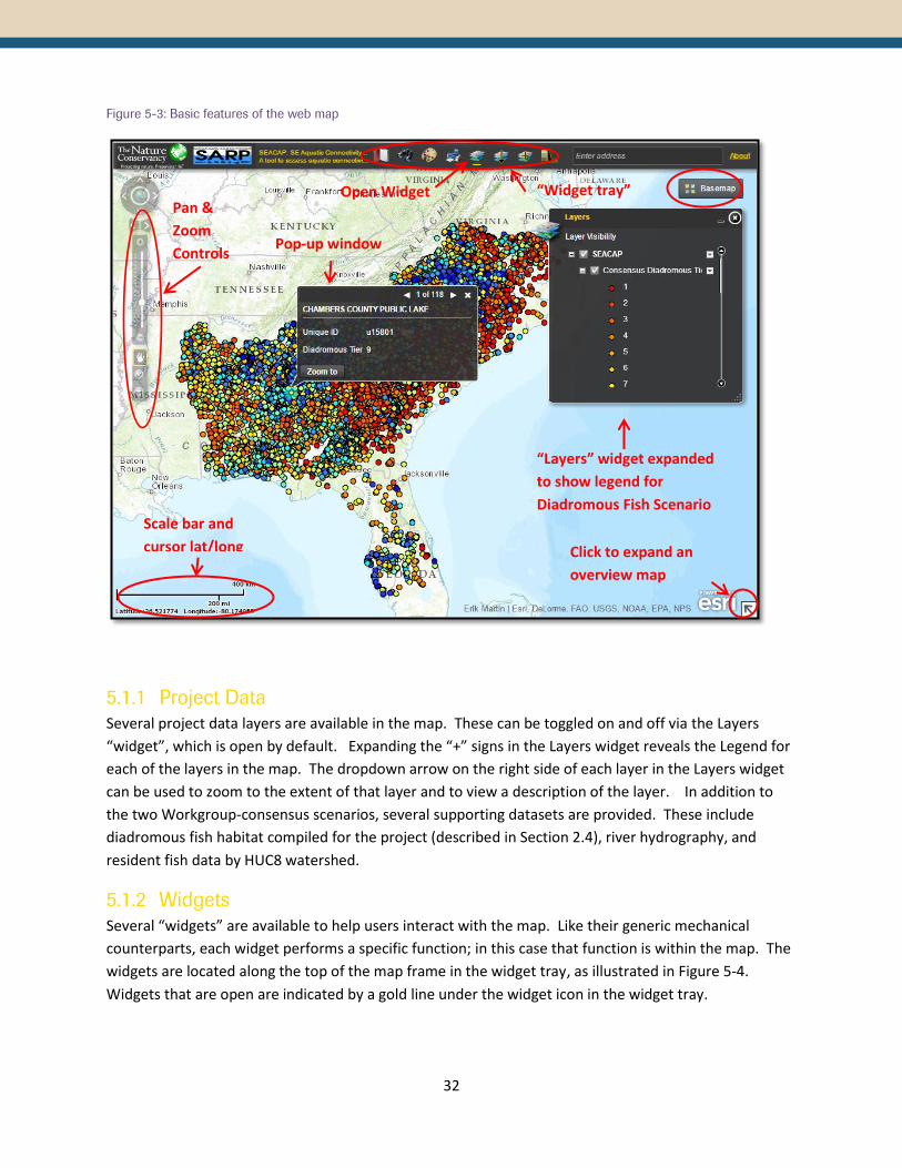
Figure 5-3: Basic features of the web map
5.1.1 Project Data
Several project data layers are available in the map. These can be toggled on and off via the Layers
“widget”, which is open by default. Expanding the “+” signs in the Layers widget reveals the Legend for
each of the layers in the map. The dropdown arrow on the right side of each layer in the Layers widget
can be used to zoom to the extent of that layer and to view a description of the layer. In addition to
the two Workgroup-consensus scenarios, several supporting datasets are provided. These include
diadromous fish habitat compiled for the project (described in Section 2.4), river hydrography, and
resident fish data by HUC8 watershed.
5.1.2 Widgets
Several “widgets” are available to help users interact with the map. Like their generic mechanical
counterparts, each widget performs a specific function; in this case that function is within the map. The
widgets are located along the top of the map frame in the widget tray, as illustrated in Figure 5-4.
Widgets that are open are indicated by a gold line under the widget icon in the widget tray.
Pop-up window
“Layers” widget expanded
to show legend for
Diadromous Fish Scenario
“Widget tray”
Scale bar and
cursor lat/long
Click to expand an
overview map
Pan &
Zoom
Controls
Open Widget

33
Figure 5-4: Widgets in the Widget Tray
5.1.2.1 Bookmark
The Bookmark widget allows users to zoom to predefined map extents such as a state boundary. Users
can also define and save the current map extent as a bookmark to easily return to later. However, these
user-defined bookmarks do not persist between sessions.
5.1.2.2 Search
The Search widget can be used to locate dams by name, by SEACAP Unique ID, or graphically. To search
for a dam by name, simply open the widget and enter all or part of a dam name, as depicted in Figure
5-5. The “text search” option to search by name is enabled by default when the widget is opened.

34
Figure 5-5: Search widget- find a dam by name.
To search for dams graphically, select the “Graphical Search” icon at the top of the widget. Drawing
tools can then be used with your mouse pointer to draw a box around a set of dams, for example, and
retrieve a table of attributes for these dams. Additional information about the Search widget can be
found at http://www.arcgis.com/home/item.html?id=5d4995ccdb99429185dfd8d8fb2a513e.
5.1.2.3 Draw
The Draw widget can be used to annotate a map with text or drawings. Several options are available to
customize the look of drawings
including fill color, outline
color, and transparency (alpha).
An option is also available to
display measurements for
drawings. Preferred units and
fonts can be set if
measurements are included.
Drawings can be saved and
shared or re-loaded into
another map session. They will
also be included if the map is
saved (PDF) or printed via the
Print widget.
Text Search
Graphical search
Figure 5-6: The Draw widget

35
5.1.2.4 Print
The Print widget allows the user to print the current map view, formatted as the map window only or to
the selected size with border information (legend, scale bar, etc.) included. It can be saved as a PDF or
image file (JPG, PNG). The result is opened as a new tab or window in the user’s browser, whence it can
be saved to the desired location.
5.1.2.5 Layers
The Layers widget is open by default when the map loads. Individual layers can be turned on and off by
checking or unchecking the box for each
layer. If a layer is part of a grouped
layer, the box for the group must be
checked in order for the layer to be
visible in the map. Expanding the check
boxes for each layer reveals any nested
layers and displays the symbology if
there are no nested layers. The drop-
down arrow on the right side of each
layer name allows users to zoom to the
extent of the layer and view a brief
description of the layer. These features
are illustrated inFigure 5-7.
Figure 5-7: The Layers widget

36
5.1.2.6 Extract & Download Data
The Extract & Download Data widget allows users to download all or a portion of the project results and
dam data. First, a tool is selected to define an area of interest. If all of the dam data is desired, simply
draw a box around the entire project area. Next, the data layers of interest are selected. Choices
include the two consensus prioritization scenarios as well as the dam data with all of the metric
attributes included. Finally the data format is selected. Choices include shapefiles or ESRI File
Geodatabase.
5.1.2.7 Additional Map Layers
Users have the option to add map services, or a data layer that can be consumed by web mapping
applications, from other
sources. These map
services are publicly
available services which
have thematic relevance to
SEACAP, but are not
directly associated with
SEACAP. Selecting the
“Additional Map Layers”
widget will open a dialog
with a list of possible map
services. A map service
may contain one or more
Select layer
Select the
output data
format
Choose a
shape to
define the
area of
interest
Figure 5-8: Extract & Download Data widget
Figure 5-9: The additional Map Layers widget

37
individual layers within it. Simply select a map service and click the “Load” button to add the new layers
to the map. The “Layers” widget will reflect the addition of the new map layers.
5.1.2.8 Custom Dam Prioritization
The Custom Dam Prioritization tool (widget) was developed for SEACAP to allow on-the-fly
prioritizations based on user-specified metric weights. Further explanation of the Custom Dam
Prioritization tool is in Section 5.2.
5.2 Custom Dam Prioritization Tool The Custom Dam Prioritization tool (or the “Tool”) allows users to modify and build off of the two
scenarios developed by the SEACAP Workgroup (see Section 4.1) by altering metric weights, filtering the
input dams (e.g. by state or watershed), and running “removal scenarios” as if one or more dams had
been removed from the network.
The Tool exists in four different states: Inputs, Status, Results, and Summary Statistics. The Inputs state
is open by default and is the interface through which the user inputs all desired parameters. When all
inputs are entered and processing has begun, the Tool will automatically switch to the Status state to
report information on the status of the processing. When it is finished, it will automatically switch to
the Results state, which displays a table of Attribute information for the custom prioritization results.
Additional information on interacting with the Results is in Section 5.2.5.1. Finally, the Summary
Statistics state displays a table of optional summary statistics, if they were calculated (See Section 5.2.3).
Although the Tool will automatically switch between states at key times, the user can select a given
state at any time by using the radio buttons along the top of the Tool.
Hovering the mouse over most items in the Tool summons tool tips – short descriptions of that button,
input, or other feature. The tool tips contain instructions and other useful information. Descriptions of
each metric can be found by clicking on the metric name. This will open a link to a PDF file which
contains a full glossary of all metrics.
The basic features of the Custom Dam Prioritization tool are illustrated in Figure 5-10.
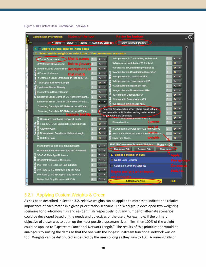
38
Figure 5-10: Custom Dam Prioritization Tool layout
5.2.1 Applying Custom Weights & Order
As has been described in Section 3.2, relative weights can be applied to metrics to indicate the relative
importance of each metric in a given prioritization scenario. The Workgroup developed two weighting
scenarios for diadromous fish and resident fish respectively, but any number of alternate scenarios
could be developed based on the needs and objectives of the user. For example, if the primary
objective of a user was to open up the most possible upstream river miles, then 100% of the weight
could be applied to “Upstream Functional Network Length.” The results of this prioritization would be
analogous to sorting the dams so that the one with the longest upstream functional network was on
top. Weights can be distributed as desired by the user so long as they sum to 100. A running tally of
States of the tool
Resize for laptops
Example tool tip
Begins analysis when inputs
are complete
Apply
Workgroup-
Consensus
Weights
Metric names
link to glossary
descriptions of
that metric
Current
sum of
metric
weights
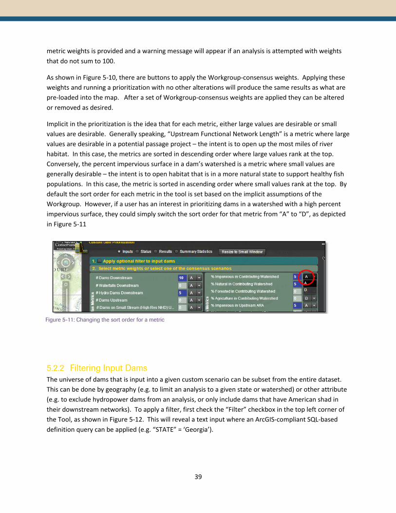
39
metric weights is provided and a warning message will appear if an analysis is attempted with weights
that do not sum to 100.
As shown in Figure 5-10, there are buttons to apply the Workgroup-consensus weights. Applying these
weights and running a prioritization with no other alterations will produce the same results as what are
pre-loaded into the map. After a set of Workgroup-consensus weights are applied they can be altered
or removed as desired.
Implicit in the prioritization is the idea that for each metric, either large values are desirable or small
values are desirable. Generally speaking, “Upstream Functional Network Length” is a metric where large
values are desirable in a potential passage project – the intent is to open up the most miles of river
habitat. In this case, the metrics are sorted in descending order where large values rank at the top.
Conversely, the percent impervious surface in a dam’s watershed is a metric where small values are
generally desirable – the intent is to open habitat that is in a more natural state to support healthy fish
populations. In this case, the metric is sorted in ascending order where small values rank at the top. By
default the sort order for each metric in the tool is set based on the implicit assumptions of the
Workgroup. However, if a user has an interest in prioritizing dams in a watershed with a high percent
impervious surface, they could simply switch the sort order for that metric from “A” to “D”, as depicted
in Figure 5-11
5.2.2 Filtering Input Dams
The universe of dams that is input into a given custom scenario can be subset from the entire dataset.
This can be done by geography (e.g. to limit an analysis to a given state or watershed) or other attribute
(e.g. to exclude hydropower dams from an analysis, or only include dams that have American shad in
their downstream networks). To apply a filter, first check the “Filter” checkbox in the top left corner of
the Tool, as shown in Figure 5-12. This will reveal a text input where an ArcGIS-compliant SQL-based
definition query can be applied (e.g. “STATE” = ‘Georgia’).
Figure 5-11: Changing the sort order for a metric
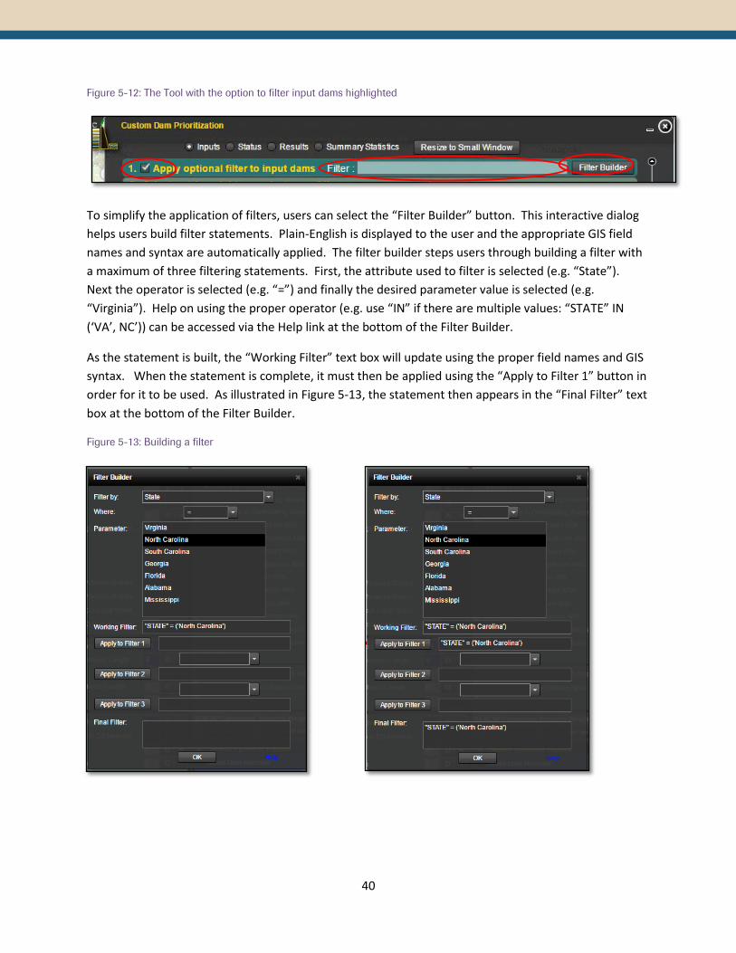
40
Figure 5-12: The Tool with the option to filter input dams highlighted
To simplify the application of filters, users can select the “Filter Builder” button. This interactive dialog
helps users build filter statements. Plain-English is displayed to the user and the appropriate GIS field
names and syntax are automatically applied. The filter builder steps users through building a filter with
a maximum of three filtering statements. First, the attribute used to filter is selected (e.g. “State”).
Next the operator is selected (e.g. “=”) and finally the desired parameter value is selected (e.g.
“Virginia”). Help on using the proper operator (e.g. use “IN” if there are multiple values: “STATE” IN
(‘VA’, NC’)) can be accessed via the Help link at the bottom of the Filter Builder.
As the statement is built, the “Working Filter” text box will update using the proper field names and GIS
syntax. When the statement is complete, it must then be applied using the “Apply to Filter 1” button in
order for it to be used. As illustrated in Figure 5-13, the statement then appears in the “Final Filter” text
box at the bottom of the Filter Builder.
Figure 5-13: Building a filter

41
If additional filters are desired, they can be developed by
repeating the process. Figure 5-14 illustrates adding a
second filter so that only dams on larger rivers are
included in the analysis. Multiple values can be selected
by holding down the Ctrl key and clicking. Another
operator is placed between the two filter statements.
The example depicted in Figure 5-14 results in the
following filter statement : "STATE" = ('North Carolina')
AND "NESZCL" IN (‘3a’ ,’3b’, ‘4’, ‘5’) , which restricts the
dams in the analysis to dams in North Carolina on rivers
that drain 200 or more square miles.
Finally, clicking on “OK” in the Filter Builder applies the
Final Filter statement to the input filter dialog on the
Tool, as depicted in Figure 5-15. Note that it is critical to
keep the check box checked if using a filter. Unchecking
it will remove the filter. Likewise, if the box is checked a
filter must be applied.
For more information on ArcGIS-compliant SQL-based
definition queries see:
http://resources.arcgis.com/en/help/main/10.2/index.html#//00s50000002t000000.
Figure 5-15: Final filter applied from the Filter Builder
5.2.3 Generating Summary Statistics
Optionally, summary statistics can be produced for the custom prioritization scenario results. These
summary statistics can be used to evaluate and make relative comparisons between watersheds or
states. If summary statistics are desired, simply check the “Calculate Summary Statistics” box towards
the bottom right corner of the Tool. This will reveal options to generate summary statistics for either
Tier or the Final Rank (the un-binned sequential results) by either State or Watershed. The output table
will enable users to makes statements such as “Watershed X has a mean Tier value of 8 while
Figure 5-14: Adding a second filter using the Filter
Builder

42
Watershed Y has a mean Tier value of 5.” From this statement we can deduce that Watershed Y has
more dams with greater potential to benefit the target of interest, based on the metric weights chosen
by the user, than Watershed X.
Figure 5-16: Selecting the option to run summary statistics on custom prioritization results
5.2.4 Dam Removal Scenarios
One or more dams can be selected for “removal” when a prioritization is run. This functionality can
allow users to assess the impact of a proposed project on the remaining dams in the network. When
dams are modeled for removal, all of the metric values are recalculated as if that dam does not exist.
To run a prioritization scenario that includes modeled removals, first check the “Model Dam Removal”
check box towards the bottom right corner of the Tool. This reveals a button to “Select Dams” as well as
a text input box (Figure 5-17). If you know the UNIQUE_ID for your dams of interest, you can simply
enter these in the text box enclosed in single quotes and separated by commas. (e.g ‘u5253’, ‘u1546’).
The UNIQUE_ID is the SEACAP project-specific identifier for each dam. It is based on the ID from the

43
source dam database, but is specific to this project. The UNIQUE_ID can be obtained by clicking on an
individual dam. Entering UNIQUE_IDs directly can be useful when running the same or similar scenarios
multiple times.
Figure 5-17: Selecting the option to model dams for removal
More convenient in many cases will be the option to select dams interactively through the web map.
This can be done by clicking on the “Select Dams” button next to the Model Dam Removal check box.
Clicking on this button prepares the Tool to interactively select dams for removal. This includes
automatically resizing the Tool and moving it to a corner of the map, turning off all map layers, and
adding a layer of all dams (symbolized as black points) that is used for selection. This process can take a
few moments, and a warning message appears to inform the user as much. This process can be sped up
by first zooming into the area of interest, thus eliminating the need for the browser to load and render
all of the dams in the region.

44
Figure 5-18: Dams ready to be selected for modeled removal
When the warning message is dismissed, users can proceed to select dams for “removal.” This is simply
done by clicking on a dam point, at which point it will turn red and its UNIQUE_ID will be populated in
the text input box. Currently, users are limited to selecting ten or fewer dams for removal to keep
processing times reasonable. If a mistake is made, clicking on a red dam will return it to black and
remove its UNIQUE_ID from the text input box.

45
Figure 5-19: A set of dams (haphazardly selected for demonstration purposes) to be modeled as removed
When finished, clicking on the “Click When Finished” button will reformat the UNIQUE_IDs into the
proper syntax, remove the selection layer from the map, and turn the other map layers back on. After
metric weights are applied, the analysis can be started by clicking the “Submit” button. When the
prioritization is complete, the values that are displayed in the Results are calculated as if the chosen
dams had been removed – this is true of the prioritization outputs (Final Rank and Tier) as well as all of
the metric values that were included in the analysis (those whose weight >0).
5.2.5 Viewing and Exporting Results
When an analysis is started, the Tool will automatically switch to the “Status” state. This state is used to
report on the progress of the prioritization. The time required to run a prioritization varies based on the
number of dams included in the analysis, the number of metrics included in the analysis, the number of
dams being modeled for removal, whether summary statistics are being calculated, as well as server
load. Generally, a custom analysis can be expected to run between 30 seconds and 2 minutes.

46
Figure 5-20: The "Status" state of the Tool displaying updates on a current analysis.
5.2.5.1 Results
Results are presented in the Results state of the Tool. When an analysis is complete the Tool will
automatically switch to this state. If any dams were selected for “removal,” a warning message will
appear to remind the user that the values presented in the Results are based on the selected dams
being removed (Figure 5-21).

47
Figure 5-21: The “Results” state with a warning message indicating which dam(s) were selected for removal.
After dismissing this warning, users enter the Results table. Similar to a desktop GIS, records in the
Results table are linked to features in the map. The Results table includes the dam name, SEACAP
Unique ID, Tiered Result (5% bins, which should be considered the “result” value), sequentially ranked
result that the 5% bins are based on, as well as the raw metric values for only those metrics that were
selected by the user. Clicking on a record in the table will highlight the dam in the map with a pulsing
red halo. Double clicking on a record will zoom to the dam in the map. Likewise, clicking on a dam in
the map will highlight the associated record in the table. Labels will appear in the map showing the
dam’s name and its result tier for the custom scenario.
Note that the map latency (response time) may increase noticeably after custom results have been
added to the map. In order to provide more functionality (specifically, the link between a dam in the
map and a corresponding result in the table) results are dynamically drawn by the client browser. Thus,
the speed which the map responds to user input (i.e. panning, zooming) will vary based on the user’s
hardware and software configuration. Because the latency is a result of the browser drawing the dam
graphics in the map, it will be more pronounced in a custom analysis that includes all the inputs dams as
opposed to an analysis that only dams includes one state, for example. If the latency is severe, it can be
managed by turning off the results layer before panning or zooming, then turning the layer back on
when the desired extent is reached.

48
Figure 5-22: Select a record in the Results to zoom to a corresponding feature highlighted in the map.
The symbols of the resulting features in the map use the same color ramp as the pre-loaded Workgroup-
consensus results to indicate Tier (Tier 1 = red, Tier 20 = blue). To help avoid confusion the default
results are automatically turned off when a custom scenario result is added to the map. The default
results can be turned back on at any time.
Any given column in the Results table can be used to sort the table. The custom result table only
includes the raw metric values for those fields that were selected by the user as weighted metrics. Data
for the other raw metrics can be obtained from the “SEACAP Dams – All Metric Data” layer in the map.
A dam & its
corresponding record
in the Results table

49
Figure 5-23: Sorting on a column in the results and buttons to work with the results.
A series of buttons along the bottom of the Results table allow users to interact with the results. From
left to right these buttons zoom to the full extent of the Study area, zoom to the extent of the custom
results, export input parameters (metric weights, filter, dams selected for removal) to a text file, export
the results table as a Microsoft Excel file, and clear the results (both the table and the features on the
map). It is strongly recommended that input parameters always be saved with results, and that the file
names be made to correspond to each other.
5.2.5.2 Summary Statistics
Optionally, summary statistics can be performed on either Tier or Final Result (the un-binned, sequential
rank) and by states or watersheds. To access the summary statistics table, select the Summary Statistics
radio button at the top of the Tool (Figure 5-24). In the example below, summary statistics are shown
by state for Tiers in an example custom analysis. Thus, all of the states in the analysis have at least one
Tier 1 dam. Similarly to the Results table, the Summary Statistics can be exported as a Microsoft Excel
(.xls) file and saved for future reference. Also, as with the results and input parameter exports, it is
strongly recommended that summary statistics are exported as an Excel file that is named to clearly
indicate from which scenario it is derived.
Arrow indicating ascending
sort order

50
Figure 5-24: Summary statistics of custom scenario results

51
Anderson, M.G., A. Barnett, M. Clark, C. Ferree, A. Olivero Sheldon, and J. Prince. 2014. Resilient Sites for Terrestrial Conservation in the Southeast Region. The Nature Conservancy, Eastern Conservation Science. 127 pp. Atlantic States Marine Fisheries Commission (ASMFC). 2004. Alexa McKerrow, Project Manager,
Biodiversity and Spatial Information Center (BaSIC) at North Carolina State University (NCSU).
Beyer, Hawthorne. 2009. Geospatial Modeling Environment (GME), version 0.3.4 Beta [software].
http://www.spatialecology.com/gme/index.htm
Collier, M., R. Webb, and J. Schmidt, Dams and rivers: Primer on the downstream effects of dams, U.S.
Geol. Surv. Circ., 1126, 1997.
Elkins, D. and N. Nibbelink. 2012. Compilation of field and GIS-based barrier assessment studies in the
Southeast Aquatic Resources Partnership (SARP) region. Warnell School of Forestry and Natural
Resources. Athens, GA
Esselman, P., D.M. Infante, D. Wieferich, A. Cooper, L. Wang, W. Taylor, R. Tingley, D. Thornbrugh, J.
Ross, and J. Fenner. (May 2013) National Fish Habitat Action Plan (NFHAP) 2010 Community Fish Data.
National Fish Habitat Partnership Data System 3.0. http://dx.doi.org/doi:10.5066/F7QN64RG
Gesch, D.B., 2007, The National Elevation Dataset, in Maune, D., ed., Digital Elevation Model Technologies and Applications: The DEM Users Manual, 2nd Edition: Bethesda, Maryland, American Society for Photogrammetry and Remote Sensing, p. 99-118. Gesch, D., Oimoen, M., Greenlee, S., Nelson, C., Steuck, M., and Tyler, D., 2002, The National Elevation Dataset: Photogrammetric Engineering and Remote Sensing, v. 68, no. 1, p. 5-11. Graf, W.L., 1999. Dam nation: a geographic census of American dams and their largescale hydrologic
impacts. Water Resources Research 35(4), 1305-1311.
Hoenke, K., Kumar, M., Batt, L. A GIS based approach for prioritizing dams for potential removal,
Ecological Engineering, Volume 64, March 2014, Pages 27-36, ISSN 0925-8574,
http://dx.doi.org/10.1016/j.ecoleng.2013.12.009.
Horizon Systems Corporation. 2012. NHDPlus Version 2. http://www.horizon-
systems.com/nhdplus/NHDPlusV2_documentation.php
Ignatius, A.R. and J. W. Jones, 2014. Small Reservoir Distribution, Rate of Construction, and Uses in the Upper and Middle Chattahoochee Basins of the Georgia Piedmont, USA, 1950–2010. International Journal of Geo-Information, 3(2): 460-480. Ignatius, A.R. and T.A. Stallins, 2011. Assessing Spatial Hydrological Data Integration to Characterize Geographic Trends in Small Reservoirs in the Apalachicola-Chattahoochee-Flint River Basin. Southeastern Geographer, 51(3): 371-393.

52
Martin, E. H. and Apse, C.D. 2013. Chesapeake Fish Passage Prioritization: An Assessment of Dams in the
Chesapeake Bay Watershed. The Nature Conservancy, Eastern Division Conservation Science.
http://maps.tnc.org/erof_ChesapeakeFPP
Martin, E. H. and C. D. Apse. 2011. Northeast Aquatic Connectivity: An Assessment of Dams on
Northeastern Rivers. The Nature Conservancy, Eastern Freshwater Program.
http://rcngrants.org/content/northeast-aquatic-connectivity
Master, Lawrence L., Stephanie R. Flack and Bruce A. Stein, eds. 1998. Rivers of Life: Critical Watersheds
for Protecting Freshwater Biodiversity. The Nature Conservancy, Arlington, Virginia
Matthews, W.J. and H.W. Robison. 1988. The distribution of fishes of Arkansas: a multivariate analysis.
Copeia :358-374.
National Elevation Dataset. United States Geological Survey. http://ned.usgs.gov/about.html
Olivero, Arlene and Anderson, Mark. 2008. Northeast Aquatic Habitat Classification System. Boston.
http://rcngrants.org/node/38
Smith, Mark; Schiff, Roy; Olivero, Arlene; and MacBroom, James. 2008. The Active River Area: A River
Conservation Framework for Protecting Rivers and Streams.
https://www.conservationgateway.org/ConservationByGeography/NorthAmerica/UnitedStates/edc/rep
ortsdata/freshwater/floodplains/Pages/default.aspx
Vannote, RL,G. W. Minshall, K. W. Cummins, J.R. Sedell, and E. Gushing 1980. The river continuum
concept. Can. J. Fish. Aquat. Sci. 37: 130-137.

53
Name Affiliation
Mark Anderson The Nature Conservancy - Eastern US Division
Colin Apse The Nature Conservancy - Eastern US Division
Analie Barnett The Nature Conservancy - Eastern US Division
Jose Barrios USFWS
Lynette Batt Unique Places, LLC (formerly American Rivers - North Carolina)
Braven Beaty The Nature Conservancy - Virginia
Rebecca Benner The Nature Conservancy - North Carolina
Walter (Tripp) Bolton USFWS - Region 4
Mary Kate Brown The Nature Conservancy - Alabama
Janet Cakir South Atlantic Landscape Conservation Cooperative
Mark Cantrell USFWS Region 4
Dan Catchings Alabama Dept. of Natural Resources
Mary Conley The Nature Conservancy - Alabama
John Damer Georgia Dept. of Natural Resources
Will Duncan USFWS Region 4
Duncan Elkins University of Georgia
Kathleen Freeman The Nature Conservancy - Florida
Mary Freeman US Geological Survey - Georgia
Paul Freeman The Nature Conservancy - Alabama
Nate Gillespie US Forest Service - Fisheries Program
Lisa Gordon Environmental Protection Agency Region 4
Sara Gottlieb The Nature Conservancy - Georgia
Chris Goudreau North Carolina Wildlife Resources Commission
Will Graf The Nature Conservancy - SC / University of South Carolina
Emily Granstaff Southeast Aquatic Resources Partnership
Emily Greene NOAA Marine Habitat Program
Kale Gullett Natural Resources Conservation Service
Kevin Hart North Carolina Division of Marine Fisheries
Lisa Havel Atlantic States Marine Fisheries Commission
Brent Hess Georgia Dept. of Natural Resources
Ted Hoehn Florida Fish & Wildlife Commission
Kat Hoenke Southeast Aquatic Resources Partnership
Chad Holbrook South Carolina Dept. of Natural Resources
Carol Johnston Auburn University (Alabama)
John Kauffman Southeast Aquatic Resources Partnership
Jeff Kipp Atlantic States Marine Fisheries Commission
Eric Krueger The Nature Conservancy - South Carolina

54
Name Affiliation
Christi Lambert The Nature Conservancy - Georgia
Wilson Laney USFWS Region 4
Erik Martin The Nature Conservancy - Eastern US Division
Brad Maurer The Nature Conservancy - Mississippi
Erin McCombs American Rivers
Keith McFadden US Geological Survey - NHD
Kevin Moody Federal Highway Administration
Rua Mordecai USFWS - South Atlantic Landscape Conservation Cooperative
Lisa Moss USFWS - Virginia Fisheries
January Murray Georgia Dept. of Natural Resources
Robert Newton The Nature Conservancy - South Carolina
Arlene Olivero Sheldon The Nature Conservancy - Eastern US Division
Pat O'Neil Geological Survey of Alabama
Bill Post South Carolina Dept. of Natural Resources
Jeff Powell USFWS - Daphne, Alabama
Peter Raabe American Rivers
Kathy Rawls North Carolina Division of Marine Fisheries
Fritz Rhode NOAA Atlantic Branch (NC)
Scott Robinson Southeast Aquatic Resources Partnership
Mark Scott South Carolina Dept. of Natural Resources
Kristina Serbesoff-King The Nature Conservancy - Florida
Tyler Stubbs Mississippi Division of Wildlife, Fisheries, and Parks
Alan Weaver Virginia Dept. of Game and Inland Fisheries
Mike Wicker USFWS - North Carolina Coastal Program
Daniel Wieferich US Geological Survey
Bennett Wynne North Carolina Wildlife Resources Commission
Jerry Ziewitz USFWS Region 4

55
Dataset Source Description
Dams Multiple sources including: state agencies, UGA SSBGIS, NC BPT, the National Inventory of Dams, National Anthropogenic Barrier Dataset, NHD Dam Events, and edited dams. Review and edits made by the SEACAP Workgroup
This dataset represents dams in the SALCC region that are spatially linked to the stream flowline in the NHDPlus v2 dataset. Dams that do not fall on mapped streams in the NHDPlus v2 are not included in the results. Complete metadata is available via http://maps.tnc.org/seacap/assets/metadata/SEACAP_damsMetrics.xml
Waterfalls USGS GNIS database, SEACAP Workgroup. USGS draft data (Daniel Wieferich, personal communication)
Point dataset representing potential natural barriers to fish passage. Waterfalls were used in the development of functional river networks, but are not included in the prioritization results as potential candidates for fish passage projects.
Hydrography NHDPlus version 2 In order for dams to be included in the analysis, they had to fall on the mapped river network, or hydrography, that was used in the project: a modified version of the Medium Resolution National Hydrography Dataset Plus, Version 2 (NHDPlus v2) (Horizon Systems 2012). This hydrography was originally digitized by the United States Geological Survey primarily from 1:100,000 scale topographic maps. Substantial additions and improvements were applied to the USGS NHD data by Horizon Systems Corporation to create the NHDPlus v2. In order to be used in this analysis the hydrography had to be processed to create a dendritic network, or dendrite: a single-flowline network with no braids or other downstream bifurcation (Figure 2-4). The medium-resolution NHDPlus used in this project includes attributes which were used to select the mainstem of a river from a braided section using a simple definition query to extract a dendrite. (NHDFlowline.FLOWDIR = 'With Digitized' AND NHDPlusFlowlineVAA.Divergence in (0,1) AND NHDPlusFlowlineVAA.StreamCalc <>0). Additional information on the NHDPlus v2 and these attributes can be found in the NHDPlus v2 User Guide (Horizon Systems 2012).
Diadromous fish habitat
Data was from ASMFC, NFHAP, MARIS, and expert knowledge
Critical habitats (spawning, nursery or other critical habitats) assigned to segments of the project hydrography. Segments needed to reach the uppermost documented location for alewife, blueback herring, American shad, hickory shad, Alabama Shad, Atlantic sturgeon, Gulf sturgeon,

56
striped bass, and American eel. Active River Area
Smith et al. 2008 The Active River Area (ARA) is a spatially explicit framework for modeling rivers and their dynamic interaction with the land through which they flow (Smith et al. 2008). Key features of the ARA include the meander belt, riparian wetlands, floodplains, terraces, material contribution areas. The ARA is different from, but was calibrated to and compared against the FEMA 100‐year floodplain. The SEACAP project used the ARA as a unit within which various landcover metrics, such as forest cover and impervious surface, were summarized.
Land Cover 2011 National land Cover Database (NLCD2011)
Land use / land cover data from the NLCD2011. This 30m gridded data was grouped into natural and agricultural. (Developed was addressed via the impervious surface data). Natural landcover includes the following classes: open water, barren land, deciduous forest, evergreen forest, mixed forest, scrub/shrub, grassland/herbaceous, woody wetlands, emergent wetlands. Agricultural includes the following classes: pasture/hay, cultivated crops. The percentages of both agricultural and natural land cover are assessed for the contributing watershed of each dam, as well as within the active river area of the dam's upstream and downstream networks.
Impervious Surface
2011 National land Cover Database (NLCD2011)
% Impervious surface data from the NLCD2011. This 30m gridded data describes the % of impervious surface within each 30m cell. The percentages of impervious surface is assessed for the contributing watershed of each dam, as well as within the active river area of the dam's upstream and downstream networks.
Resident fish, rare fish, mussels & rare crayfish
NatureServeHUC8-scale data USGS BISON point observations MARIS point observations
Data for each species of interest (see Appendix 9) was assigned to HUC8s on a presence/absence basis. See Section 2.5 for more details. These metrics are available for custom prioritizations
Invasive Species
NatureServeHUC8-scale data USGS BISON point observations MARIS point observations
Data for each species of interest (see Appendix 9) was assigned to HUC8s on a presence/absence basis. See Section 2.5.2 for more details. These metrics are available for custom prioritizations
Roads and Railroads
Esri version 10.1 data Roads and railroads obtained from Esri's ArcGIS version 10.1 data were intersected with small streams (drainage area <38.61sq mi) as a proxy for culvert locations.

57
Conservation Land
The Nature Conservancy Dams that lie on conservation lands are identified. Additionally, the percentage of conservation land is assessed within a 100m buffer of each dam's upstream and downstream functional river networks.

58
Scientific Name
Common Name
Acipenser fulvescens Shortnose Sturgeon
Ambloplites cavifrons Roanoke Bass
Ammocrypta beanii Naked Sand Darter
Ammocrypta bifascia Florida Sand Darter
Ammocrypta meridiana Southern Sand Darter
Ammocrypta vivax Scaly Sand Darter
Campostoma anomalum Central Stoneroller
Campostoma oligolepis Largescale Stoneroller
Campostoma pauciradii Bluefin Stoneroller
Campostoma pullum Central Stone Roller Subspecies
Carassius auratus Goldfish
Chrosomus oreas Mountain Redbelly Dace
Clinostomus funduloides Rosyside Dace
Crystallaria asprella Crystal Darter
Ctenopharyngodon idella Grass Carp
Ctenopharyngodon idella trip Grass Carp
Cyprinella analostana Satinfin Shiner
Cyprinella caerulea Blue Shiner
Cyprinella callisema Ocmulgee Shiner
Cyprinella callistia Alabama Shiner
Cyprinella callitaenia Bluestripe Shiner
Cyprinella camura Bluntface Shiner
Cyprinella cercostigma Eastern Blacktail Shiner
Cyprinella chloristia Greenfin Shiner
Cyprinella galactura Whitetail Shiner
Cyprinella gibbsi Tallapoosa Shiner
Cyprinella hybrid Cyprinella labrosa Thicklip Chub
Cyprinella leedsi Bannerfin Shiner
Cyprinella lutrensis Red Shiner
Cyprinella nivea Whitefin Shiner
Cyprinella pyrrhomelas Fieryblack Shiner
Cyprinella sp 1 Cyprinella spiloptera Spotfin Shiner
Cyprinella spp Cyprinella stigmatura Regal Shiner
Cyprinella trichroistia Tricolor Shiner
Cyprinella venusta Blacktail Shiner

59
Scientific Name
Common Name
Cyprinella whipplei Steelcolor Shiner
Cyprinella xaenura Altamaha Shiner
Cyprinella zanema Santee Chub
Cyprinus carpio Common Carp
Ericymba amplamala Silverjaw Minnow
Erimystax cahni Slender Chub
Erimystax dissimilis Streamline Chub
Erimystax insignis Blotched Chub
Erimyzon oblongus Creek Chubsucker
Erimyzon tenuis Sharpfin Chubsucker
Etheostoma artesiae Redspot Darter
Etheostoma bellator Warrior Darter
Etheostoma blennioides Greenside Darter
Etheostoma brevirostrum Holiday Darter
Etheostoma brevispinum Carolina Fantail Darter
Etheostoma caeruleum Rainbow Darter
Etheostoma chermocki Vermillion Darter
Etheostoma chlorobranchium Greenfin Darter
Etheostoma chlorosoma Bluntnose Darter
Etheostoma chlorosomum Bluntnose Darter
Etheostoma chuckwachatte Lipstick Darter
Etheostoma collis Carolina Darter
Etheostoma colorosum Coastal Darter
Etheostoma coosae Coosa Darter
Etheostoma davisoni Choctawhatchee Darter
Etheostoma ditrema Coldwater Darter
Etheostoma douglasi Tuscaloosa Darter
Etheostoma edwini Brown Darter
Etheostoma etowahae Etowah Darter
Etheostoma flabellare Fantail Darter
Etheostoma fricksium Savannah Darter
Etheostoma fusiforme Swamp Darter
Etheostoma gracile Slough Darter
Etheostoma histrio Harlequin Darter
Etheostoma hopkinsi Christmas Darter
Etheostoma inscriptum Turquoise Darter
Etheostoma jessiae Blueside Darter
Etheostoma jordani Greenbreast Darter
Etheostoma lachneri Tombigbee Darter
Etheostoma lynceum Brighteye Darter
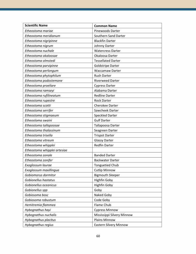
60
Scientific Name
Common Name
Etheostoma mariae Pinewoods Darter
Etheostoma meridianum Southern Sand Darter
Etheostoma nigripinne Blackfin Darter
Etheostoma nigrum Johnny Darter
Etheostoma nuchale Watercress Darter
Etheostoma okaloosae Okaloosa Darter
Etheostoma olmstedi Tessellated Darter
Etheostoma parvipinne Goldstripe Darter
Etheostoma perlongum Waccamaw Darter
Etheostoma phytophilum Rush Darter
Etheostoma podostemone Riverweed Darter
Etheostoma proeliare Cypress Darter
Etheostoma ramseyi Alabama Darter
Etheostoma rufilineatum Redline Darter
Etheostoma rupestre Rock Darter
Etheostoma scotti Cherokee Darter
Etheostoma serrifer Sawcheek Darter
Etheostoma stigmaeum Speckled Darter
Etheostoma swaini Gulf Darter
Etheostoma tallapoosae Tallapoosa Darter
Etheostoma thalassinum Seagreen Darter
Etheostoma trisella Trispot Darter
Etheostoma vitreum Glassy Darter
Etheostoma whipplei Redfin Darter
Etheostoma whipplei artesiae Etheostoma zonale Banded Darter
Etheostoma zonifer Backwater Darter
Exoglossum laurae Tonguetied Chub
Exoglossum maxillingua Cutlip Minnow
Gobiomorus dormitor Bigmouth Sleeper
Gobionellus hastatus Highfin Goby
Gobionellus oceanicus Highfin Goby
Gobionellus spp Goby
Gobiosoma bosc Naked Goby
Gobiosoma robustum Code Goby
Hemitremia flammea Flame Chub
Hybognathus hayi Cypress Minnow
Hybognathus nuchalis Mississippi Silvery Minnow
Hybognathus placitus Plains Minnow
Hybognathus regius Eastern Silvery Minnow
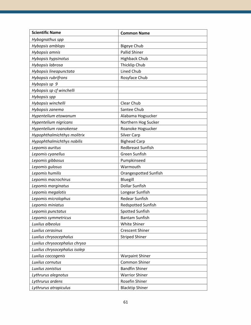
61
Scientific Name
Common Name
Hybognathus spp Hybopsis amblops Bigeye Chub
Hybopsis amnis Pallid Shiner
Hybopsis hypsinotus Highback Chub
Hybopsis labrosa Thicklip Chub
Hybopsis lineapunctata Lined Chub
Hybopsis rubrifrons Rosyface Chub
Hybopsis sp 9 Hybopsis sp cf winchelli Hybopsis spp Hybopsis winchelli Clear Chub
Hybopsis zanema Santee Chub
Hypentelium etowanum Alabama Hogsucker
Hypentelium nigricans Northern Hog Sucker
Hypentelium roanokense Roanoke Hogsucker
Hypophthalmichthys molitrix Silver Carp
Hypophthalmichthys nobilis Bighead Carp
Lepomis auritus Redbreast Sunfish
Lepomis cyanellus Green Sunfish
Lepomis gibbosus Pumpkinseed
Lepomis gulosus Warmouth
Lepomis humilis Orangespotted Sunfish
Lepomis macrochirus Bluegill
Lepomis marginatus Dollar Sunfish
Lepomis megalotis Longear Sunfish
Lepomis microlophus Redear Sunfish
Lepomis miniatus Redspotted Sunfish
Lepomis punctatus Spotted Sunfish
Lepomis symmetricus Bantam Sunfish
Luxilus albeolus White Shiner
Luxilus cerasinus Crescent Shiner
Luxilus chrysocephalus Striped Shiner
Luxilus chrysocephalus chryso Luxilus chrysocephalus isolep Luxilus coccogenis Warpaint Shiner
Luxilus cornutus Common Shiner
Luxilus zonistius Bandfin Shiner
Lythrurus alegnotus Warrior Shiner
Lythrurus ardens Rosefin Shiner
Lythrurus atrapiculus Blacktip Shiner

62
Scientific Name
Common Name
Lythrurus bellus Pretty Shiner
Lythrurus fasciolaris Scarlet Shiner
Lythrurus fumeus Ribbon Shiner
Lythrurus lirus Mountain Shiner
Lythrurus matutinus Pinewoods Shiner
Lythrurus roseipinnis Cherryfin Shiner
Lythrurus spp Lythrurus umbratilis Redfin Shiner
Macrhybopsis aestivalis Speckled Chub
Macrhybopsis hyostoma Shoal Chub
Macrhybopsis meeki Sicklefin Chub
Macrhybopsis sp 1 Macrhybopsis sp 2 Macrhybopsis spp Macrhybopsis storeriana Silver Chub
Margariscus margarita Pearl Dace
Micropterus cataractae Micropterus coosae Redeye Bass
Micropterus henshalli Alabama Bass
Micropterus notius Suwannee Bass
Micropterus punctulatus Spotted Bass
Micropterus salmoides Largemouth Bass
Moxostoma anisurum Silver Redhorse
Moxostoma ariommum Bigeye Jumprock
Moxostoma breviceps Smallmouth Redhorse
Moxostoma carinatum River Redhorse
Moxostoma cervinum Blacktip Jumprock
Moxostoma collapsum Notchlip Redhorse
Moxostoma duquesnei Black Redhorse
Moxostoma duquesnii Black Redhorse
Moxostoma erythrurum Golden Redhorse
Moxostoma lachneri Greater Jumprock
Moxostoma macrolepidotum Shorthead Redhorse
Moxostoma n sp cpoeciluru Moxostoma pappillosum V-Lip Redhorse
Moxostoma poecilurum Blacktail Redhorse
Moxostoma robustum Robust Redhorse
Moxostoma rupiscartes Striped Jumprock
Moxostoma sp 1 Moxostoma sp 3

63
Scientific Name
Common Name
Moxostoma sp 4 Moxostoma sp apalachicola re Sicklefin Redhorse
Moxostoma sp c erythrurum Golden Redhorse
Moxostoma sp c lachneri Greater Jumprock
Moxostoma spp Nocomis effusus Redtail Chub
Nocomis leptocephalus Bluehead Chub
Nocomis leptocephalus bellicu Bluehead Chub
Nocomis micropogon River Chub
Nocomis platyrhynchus Bigmouth Chub
Nocomis raneyi Bull Chub
Nocomis spp Notemigonus crysoleucas Golden Shiner
Notropis alborus Whitemouth Shiner
Notropis altipinnis Highfin Shiner
Notropis ammophilus Orangefin Shiner
Notropis amoenus Comely Shiner
Notropis amplamala Longjaw Minnow
Notropis ariommus Popeye Shiner
Notropis asperifrons Burrhead Shiner
Notropis atherinoides Emerald Shiner
Notropis baileyi Rough Shiner
Notropis bifrenatus Bridle Shiner
Notropis blennius River Shiner
Notropis boops Bigeye Shiner
Notropis buccatus Silverjaw Minnow
Notropis buchanani Ghost Shiner
Notropis cahabae Cahaba Shiner
Notropis candidus Silverside Shiner
Notropis chalybaeus Ironcolor Shiner
Notropis chiliticus Redlip Shiner
Notropis chlorocephalus Greenhead Shiner
Notropis chrosomus Rainbow Shiner
Notropis cummingsae Dusky Shiner
Notropis edwardraneyi Fluvial Shiner
Notropis harperi Redeye Chub
Notropis hudsonius Spottail Shiner
Notropis hybrid Notropis hypsilepis Highscale Shiner
Notropis leuciodus Tennessee Shiner

64
Scientific Name
Common Name
Notropis longirostris Longnose Shiner
Notropis lutipinnis Yellowfin Shiner
Notropis maculatus Taillight Shiner
Notropis mekistocholas Cape Fear Shiner
Notropis melanostomus Blackmouth Shiner
Notropis micropteryx Highland Shiner
Notropis petersoni Coastal Shiner
Notropis photogenis Silver Shiner
Notropis procne Swallowtail Shiner
Notropis rafinesquei Yazoo Shiner
Notropis rubellus Rosyface Shiner
Notropis rubricroceus Saffron Shiner
Notropis rupestris Bedrock Shiner
Notropis sabinae Sabine Shiner
Notropis scabriceps New River Shiner
Notropis scepticus Sandbar Shiner
Notropis semperasper Roughhead Shiner
Notropis shumardi Silverband Shiner
Notropis sp c N sabinae Sabine Shiner
Notropis sp c chlorocephal Greenhead Shiner
Notropis sp c rubellus Rosyface Shiner
Notropis spectrunculus Mirror Shiner
Notropis spp Notropis stilbius Silverstripe Shiner
Notropis stramineus Sand Shiner
Notropis telescopus Telescope Shiner
Notropis texanus Weed Shiner
Notropis uranoscopus Skygazer Shiner
Notropis volucellus Mimic Shiner
Notropis wickliffi Channel Shiner
Notropis xaenocephalus Coosa Shiner
Noturus sp 2 Opsopoeodus emiliae Pugnose Minnow
Percina antesella Amber Darter
Percina aurantiaca Tangerine Darter
Percina aurolineata Goldline Darter
Percina aurora Pearl Darter
Percina austroperca Southern Logperch
Percina brevicauda Coal Darter
Percina burtoni Blotchside Logperch

65
Scientific Name
Common Name
Percina caprodes Logperch
Percina caprodes caprodes Logperch
Percina copelandi Channel Darter
Percina crassa Piedmont Darter
Percina evides Gilt Darter
Percina gymnocephala Appalachia Darter
Percina jenkinsi Conasauga Logperch
Percina kathae Mobile Logperch
Percina kusha Brindled Darter
Percina lenticula Freckled Darter
Percina macrocephala Longhead Darter
Percina maculata Blackside Darter
Percina nevisense Chainback Darter
Percina nigrofasciata Blackbanded Darter
Percina notogramma Stripeback Darter
Percina oxyrhynchus Sharpnose Darter
Percina palmaris Bronze Darter
Percina peltata Shield Darter
Percina rex Roanoke Logperch
Percina roanoka Roanoke Darter
Percina sciera Dusky Darter
Percina shumardi River Darter
Percina sipsi Bankhead Darter
Percina smithvanizi Muscadine Darter
Percina sp muscadine darter Muscadine Darter
Percina squamata Olive Darter
Percina suttkusi Gulf Logperch
Percina vigil Saddleback Darter
Phenacobius catostomus Riffle Minnow
Phenacobius crassilabrum Fatlips Minnow
Phenacobius mirabilis Suckermouth Minnow
Phenacobius teretulus Kanawha Minnow
Phenacobius uranops Stargazing Minnow
Phoxinus cumberlandensis Blackside Dace
Phoxinus erythrogaster Southern Redbelly Dace
Phoxinus oreas Mountain Redbelly Dace
Phoxinus tennesseensis Tennessee Dace
Pimephales notatus Bluntnose Minnow
Pimephales promelas Fathead Minnow

66
Scientific Name
Common Name
Pimephales spp Pimephales vigilax Bullhead Minnow
Pimephales vigilax perspicuus Polyodon spathula Paddlefish
Pteronotropis euryzonus Broadstripe Shiner
Pteronotropis grandipinnis Apalachee Shiner
Pteronotropis hypselopterus Sailfin Shiner
Pteronotropis merlini Orangetail Shiner
Pteronotropis metallicus Metallic Shiner
Pteronotropis signipinnis Flagfin Shiner
Pteronotropis stonei Lowland Shiner
Pteronotropis welaka Bluenose Shiner
Rhinichthys atratulus Eastern Blacknose Dace
Rhinichthys cataractae Longnose Dace
Rhinichthys obtusus Western Blacknose Dace
Salvelinus fontinalis Brook Trout
Semotilus atromaculatus Creek Chub
Semotilus corporalis Fallfish
Semotilus lumbee Sandhills Chub
Semotilus thoreauianus Dixie Chub
Thoburnia hamiltoni Rustyside Sucker
Thoburnia rhothoeca Torrent Sucker

67
SEACAP Dam Merging Methods Kat Hoenke GOAL: To create a comprehensive and spatially accurate database of dams for the SEACAP study area using national and state datasets, while eliminating duplicates and retaining the most accurate information. Data Sources National Datasets: National Anthropogenic Barrier Dataset (NABD): This dataset is a spatially accurate dataset where NID 2009 dams were snapped to the medium resolution of NHD plus version 1. NHD dam events: These dams are point events found on the NHD plus high resolution river 1:24000 NID 2013: This is the latest version of the National Inventory of Dams, downloaded on May 5, 2013. State Datasets: Georgia EPA- From SSBGIS, a dataset compiled by Duncan Elkins. Georgia Dam Safety- From the Georgia dam safety office Tallapoosa impoundments- These dams are from Georgia and Alabama. From SSBGIS, a dataset compiled by Duncan Elkins. Florida EPA- From SSBGIS, a dataset compiled by Duncan Elkins. Florida Water Management FL Impoundments added 12-3-13 Alabama Shelby County Alabama Tuscaloosa County Alabama Jefferson County Alabama St. Clair County Alabama Blount County Alabama Marshall County Alabama Etowah County AL Impoundments added 12-3-13 NC VA Coastal – These dams are coast wide, from multiple state sources. From NC division of Marine Fisheries NC Dam Safety- From the North Carolina dam safety office 2012 and 2013

68
SC Dam Safety – From Upstate Forever, John Tynan VA Dam Safety- From the Virginia dam safety office Duplicate Removal Methods National dataset Methods: Goal: Keep all snapped dams, retain any new dams, code all duplicates. 1) Keep all dams from the NABD dataset to maintain snapping. Join in more current attributes using NID 2013. 2) If no NABD dam is available, keep all dams from NHD dam events. Join in current attributes using NID 2013. 3) Retained any NHD dam events or NID 2013 dams that did not overlap with NABD as new individual dams. 4) Possible duplicates coded as NABD or NHD dam event dikes removed 5) Coded national sources of dams within 100m of one another. 6) Coded dams within 500m of one another with similar names. State dataset methods: Goal: Keep all state dams that are not duplicates with national datasets. 1) State dams with a common NID or state ID in a national dataset were coded as duplicates 2) State dams that were within 100m (or a greater distance, if visual inspection showed more duplicates) of national dams were also coded as duplicates. Additional actions taken: 1. Pre- Snap all dams on NABD and NHD dam events with matching reachcodes (Y in snapto100k field). Snap all dams within 100m to flowline, assuming they are in the correct location. USE field: 1 = snapped dam 2 = unsnapped dam 0 = duplicate dam or other excluded dam DUPLICATE_CODES field: 0 - Non duplicate – Given 1 or 2 in USE field, depending on snapping. 1 - State duplicate common national NIDID, also within 100m of national dam -Given 0 in USE field 2 - State duplicate common national NIDID, further than 100m from a national dam-Given 0 in USE field 3 - State duplicate, within 100m of national dam. NIDID is not common. Given 0 in USE field 4 - State duplicate, within 100m of national dam. No NIDID present. Given 0 in USE field 6 - State duplicate, within 100m of another state dam with better location/attributes. Given 0 in USE field 7 - National duplicate within 100m of a snapped NABD dam. Given 0 in USE field 8 - Unsnapped dams within 100m of another dam. Contains duplicates and originals. Given 2 in USE field. 9 - Snapped dams within 100m of another dam. Contains duplicates and originals. Given 1 in use field, needs workgroup review. 10- Duplicate dam within 500m of another dam, similar dam name. Given 0 in USE field

69
SNAP field: 1 – Is snapped by BAT and part of a snapped dataset, should be snapped 2 – is snapped by BAT 3 – Should not be snapped. 0 – is not snapped

70
The following is a glossary of metrics that were calculated for each dam in the SEACAP study area. It is
available as a PDF file with working hyperlinks at
http://maps.tnc.org/seacap/assets/Metric_Glossary.pdf. Each metric within the Custom Dam
Prioritization tool is also linked to it associated glossary slide (See Section 5.2).
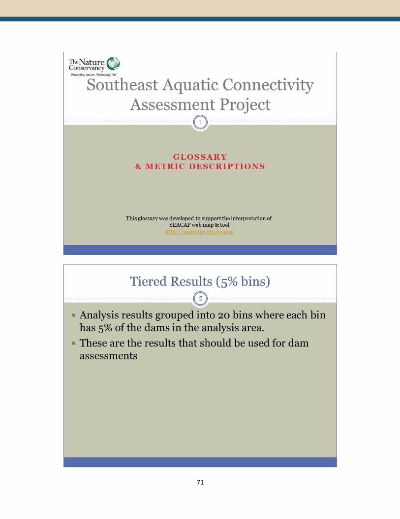
71

72

73
74

75

76

77

78

79
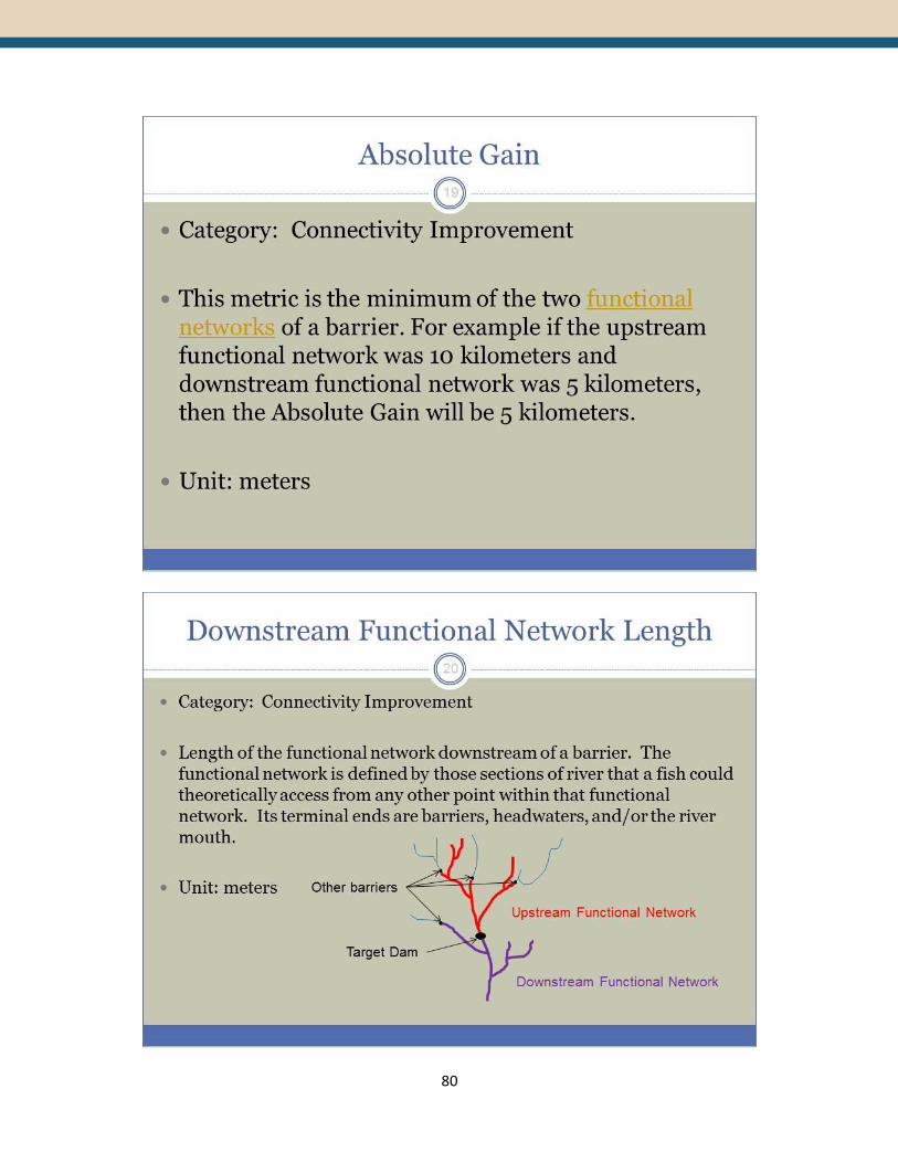
80

81

82

83

84

85

86
87

88

89
90

91

92

93

94
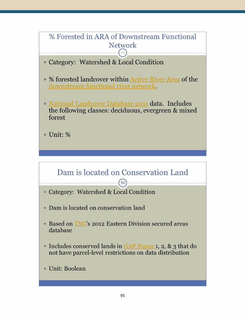
95

96
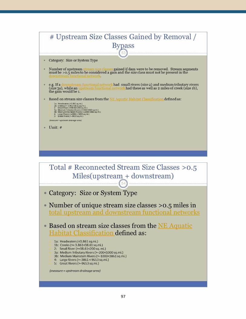
97

98