Putting computing on a strict diet with energy-proportionality

Alex Yakovlev, microSystems, School of EEE, Newcastle University

async.org.uk www.ncl.ac.uk/eee/research/groups/micro/

Power Prop

The more you get The more you give!

holistice n e r g y h a r v e s t i n g

Energy drives logic XXIX DCIS, Madrid 26th November 2014

1

Run smarter Live longer!

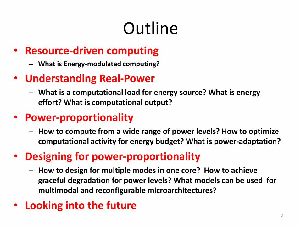
Outline • Resource-driven computing

– What is Energy-modulated computing?

• Understanding Real-Power – What is a computational load for energy source? What is energy

effort? What is computational output?

• Power-proportionality – How to compute from a wide range of power levels? How to optimize

computational activity for energy budget? What is power-adaptation?

• Designing for power-proportionality – How to design for multiple modes in one core? How to achieve

graceful degradation for power levels? What models can be used for multimodal and reconfigurable microarchitectures?

• Looking into the future 2

3

Resource-driven Computing

Energy drives logic

Energy drives logic

Energy-constrained systems

• Solar energy, e-beam power supply, small batteries, …

Unreliable power supply

• Voltage fluctuations, low battery, …

Hostile environments

• High/low temperatures, noise, …

Energy

Quality of

Service Uncertainty

Working conditions:

Interplay

4

Power/Energy modulation • The principle of power/energy-modulated computing is that the

flow of energy entering a computing system determines its computational flow

• It is fundamental for building future real-power systems, particularly systems for survivability

• Any piece of electronics becomes active and performs to a certain level of its delivered quality in response to some level of energy and power

• A quantum of energy when applied to a computational device can be converted into a corresponding amount of computation activity

• Depending on their design and implementation systems can produce meaningful activity at different power levels

• As power levels become uncertain we cannot always guarantee completely certain computational activity 5

Traditional vs energy-modulated view

6

Piezo-Film Experiment

Experiment Results

Example: Walls Alive (condition monitoring)

9

Example: condition monitoring

10

Example: condition monitoring

11

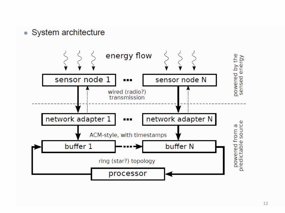
12

Power efficiency and regularity • Modern systems rely on highly regular (periodic) power sources –

they “invest” some power into power regulation • Future systems will have to operate in a wide dynamic range, paying

the price in efficiency in a particular band

13

Range of aperiodicity of power source

Power efficiency

“Narrow band” system

“Wide band” system

Highly regular (ideal) source

Sporadic (real) source

We have to learn how to compute from unregulated power sources

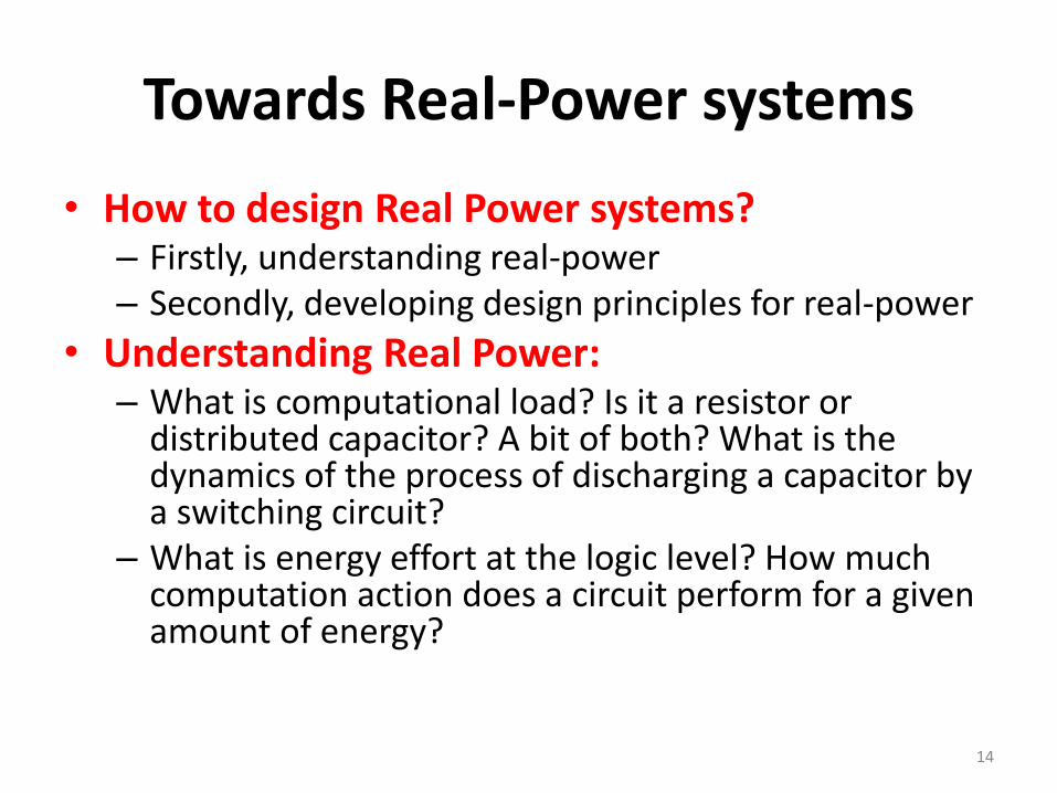
Towards Real-Power systems

• How to design Real Power systems? – Firstly, understanding real-power – Secondly, developing design principles for real-power

• Understanding Real Power: – What is computational load? Is it a resistor or

distributed capacitor? A bit of both? What is the dynamics of the process of discharging a capacitor by a switching circuit?

– What is energy effort at the logic level? How much computation action does a circuit perform for a given amount of energy?

14

Understanding Real-Power Systems

15

Ctesibius’ Clepsydra , 3rd century BC

Faraday’s homopolar motor, 1821

• We employ a simple ring-oscillator to serve as a digital circuit load.

• It is due to the fact that ring-oscillator can closely mimic the switching behaviour of many closed loop self-timed circuits.

+

C

V

Outputoscillations

16

What is Computational Load?

Circuit model

Cp

j

1→0

Cp

0→1k

C

j k

pt CN

C2

1 C

l

pt CN

C2

1 Cp

Cpt C

NC

2

1

Cp

17

Circuit Model: switching process

V0

State 3

States 1,2

Charging Cl

V1=K1 V0

V2=K2 V0

V3=K3 V0

t0 t1 t2

V drop over time

Vn=Kn V0

Discharging Cl

lCC

CVV

01

lCC

CK

n

N

n

KV

VKV

0

Charge equilibrium at:

18

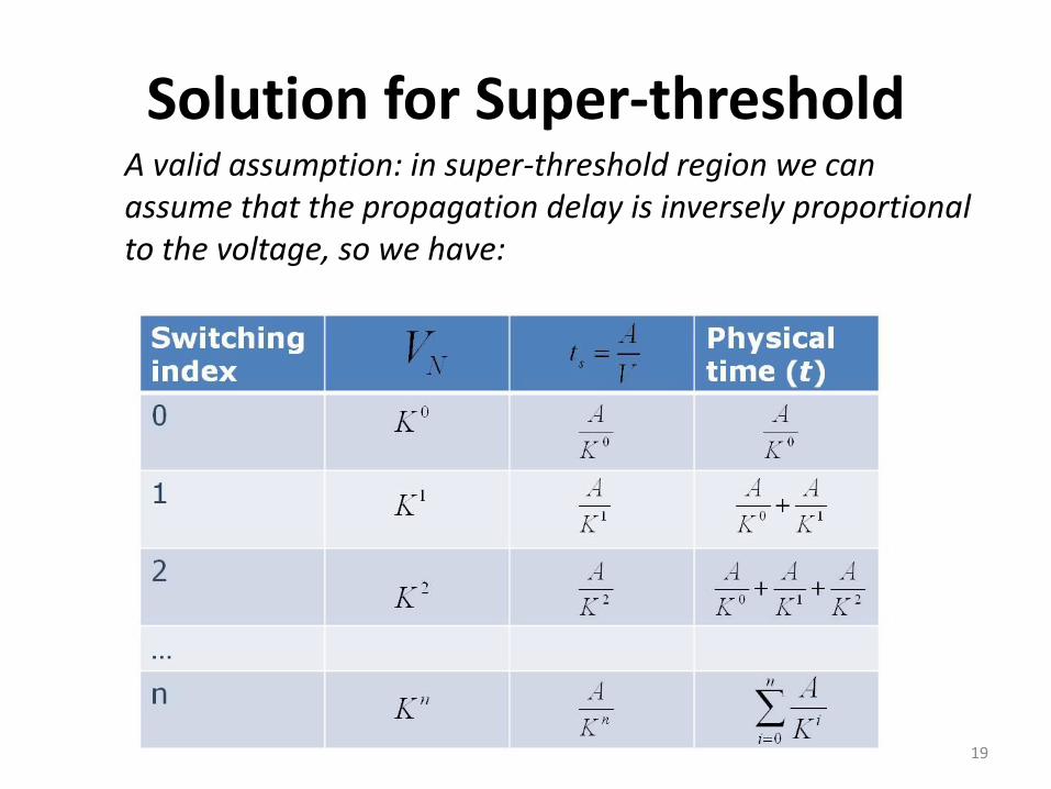
Solution for Super-threshold A valid assumption: in super-threshold region we can assume that the propagation delay is inversely proportional to the voltage, so we have:

19

Solution for Super-threshold

AKKt

AKVN

)1(Hyperbolic function of time

20

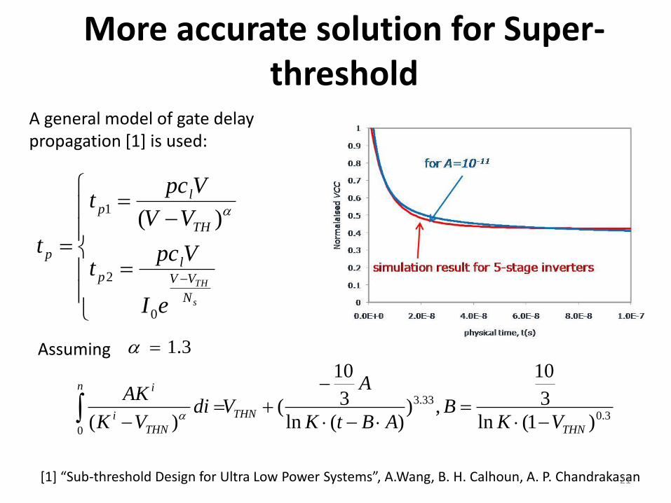
More accurate solution for Super-threshold

A general model of gate delay propagation [1] is used:

s

TH

N

VV

lp

TH

lp

p

eI

Vpct

VV

Vpct

t

0

2

1)(

3.0

33.3

0)1(ln

3

10

,))(ln

3

10

()( THN

THN

n

THN

i

i

VKB

ABtK

A

VdiVK

AK

Assuming 3.1

[1] “Sub-threshold Design for Ultra Low Power Systems”, A.Wang, B. H. Calhoun, A. P. Chandrakasan 21

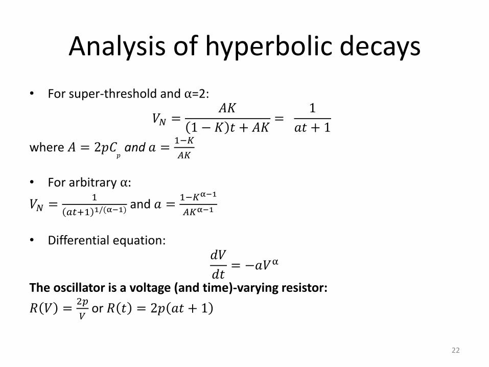
Analysis of hyperbolic decays

• For super-threshold and α=2:

𝑉𝑁 =𝐴𝐾

1 − 𝐾 𝑡 + 𝐴𝐾=

1

𝑎𝑡 + 1

where 𝐴 = 2𝑝𝐶𝑝 and 𝑎 =

1−𝐾

𝐴𝐾

• For arbitrary α:

𝑉𝑁 =1

𝑎𝑡+1 1/(α−1) and 𝑎 =1−𝐾α−1

𝐴𝐾α−1

• Differential equation:

𝑑𝑉

𝑑𝑡= −𝑎𝑉α

The oscillator is a voltage (and time)-varying resistor:

𝑅 𝑉 =2𝑝

𝑉 or 𝑅 𝑡 = 2𝑝 𝑎𝑡 + 1

22

Analysis of hyperbolic decay rates • For stack:

1

𝑎

1

α=

1

𝑎1

1

α+

1

𝑎2

1

α or

𝑎 =𝑎1𝑎2

𝑎1α + 𝑎2

αα

• For parallel: 𝑎 = 𝑎1 + 𝑎2

• Confirmed by physical experiments with discrete CMOS components:

• The value of alpha is 1.5

• The discharging process for a stack of two identical circuits is nearly 3 times slower than for a standalone circuit

23

Series (stack) and parallel configurations:

Capacitor discharge experiments

24 0 10 20 30 40 50 60

0

1

2

3

4

5

6

Time, μs

0 5 10 15 20 25 300

1

2

3

4

5

6

Time, μs

5 10 15 20 25 30

1

2

3

4

5

6

Time, μs0

0

Standalone

Parallel Stack

Reference-free voltage sensor

Data

Control

Sampling circuit

Self-timed counter

Req

E h

Ack

8

Energy harvesting source

Storage element

V dd

25

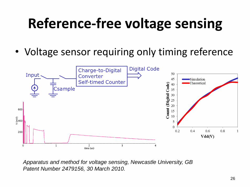
Reference-free voltage sensing

• Voltage sensor requiring only timing reference

26

Apparatus and method for voltage sensing, Newcastle University, GB

Patent Number 2479156, 30 March 2010.

Output count and energy consumption

0

10

20

30

40

50

60

70

80

0.80 1.00 1.20 1.40 1.60 1.80

Co

de

Voltage (V)

0.0E+0

5.0E-8

1.0E-7

1.5E-7

2.0E-7

2.5E-7

3.0E-7

3.5E-7

4.0E-7

0.8 1.3 1.8

Ener

gy p

er s

ensi

ng

(J)

Voltage (V)

C =10nF sample

27

Power Proportionality

28

Power Proportionality Issues reported in literature:

Source: S. Dawson-Haggerty et al. Power Optimization – Reality Check, UC Berkeley, 2009

•Performance-power tradeoff for commodity systems is linear; the best strategy is “Race to sleep”; additional “run” power states are of little use; changes in existing commodity operating systems have little influence •The focus should be on the time to transition to and from sleep! •For a new type of systems such as WSN there is a non-linear region – the slogan is: learn how to run CMOS slowly and exploit scheduling optimizations

Core i7 power drawn at different frequencies

29

Power proportionality (“knee-stretching”)

Service-modulated processing

Energy-modulated processing

30

Multiplier: Quality of Service vs Power

31

From power-proportional to power-adaptive

Power level

QoS Level

Design 1 power proportional and efficient for low power

Design 2 less power proportional and more efficient for high power

Ideally, we need a hybrid design that can adapt to available power levels!

32

Relationship with uncertainty (e.g. timing variability)

Timing robustness

Source of variability

analysis:

Yu Cao, Clark, L.T.,

2007

Technology node:

90nm

33

Towards designing power-adaptive systems

• Truly energy-modulated design must be power-adaptive

• Systems that are power adaptive are more resourceful and more resilient

• Power-adaptive systems can work in a broad range of power levels

• How to design such systems?

34

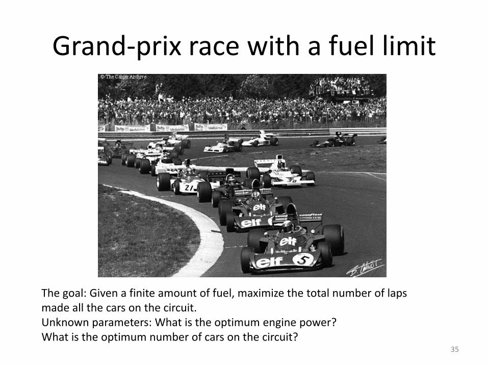
Grand-prix race with a fuel limit

35

The goal: Given a finite amount of fuel, maximize the total number of laps made all the cars on the circuit. Unknown parameters: What is the optimum engine power? What is the optimum number of cars on the circuit?

36

Ring-pipeline with a finite energy budget

Experiment: a. A ring micropipeline with 5 stages is used in the experiment. b. Simulation Results are obtained with different parallelism (1, 2, 3, 4 tokens), in different working voltages (1.0V, 0.8V, 0.6V, 0.4V, 0.35V, 0.25V, 0.2V, 0.16V), and under different amount of energy (600pJ, 700pJ, 800pJ). c. A run stops when the energy is fully consumed. d. The amount of computation is counted for each run. e. A unit of computation is defined as one pulse generated in the pipeline.

Ring pipeline with a given energy budget

37

Conclusions: • The higher the concurrency the greater the amount of computation and the smaller

the amount of leakage. • At sub-threshold voltages, the amount of computation is STRONGLY affected by

degree of concurrency, due to the effect of leakage. • Above threshold, the amount of computation that is practically insensitive to the

degree of concurrency.

Source: Akgun et al, ASYNC’10

Asynchronous (self-timed) logic can provide completion detection and thus reduce the interval of leakage to minimum, thereby doing nothing well!

Synchronous vs Self-Timed Design (in terms of energy efficiency)

Closer look at AC-powered self-timed logic

2-bit Sequential Dual-rail Asynchronous Counter

Supply: AC 200mV±100mV Frequency: 1Mhz

A1.f

A1.t

A0.f

A0.t

Self-timed logic with completion detection is robust to power supply variations

Circuit-level: speed-independent SRAM • Mismatch between delay lines and SRAM memories when

reducing Vdd

For example, under 1V Vdd, the delay of SRAM reading is equal to 50 inverters and under 190mV, the delay is equal to 158 inverters

• The problem has been well known

so far

• Existing solutions:

– Different delay lines in

different range of Vdd

– Duplicating a column of SRAM

to be a delay line to bundle the

whole SRAM

• The solutions require:

– voltage references

– DC-DC adaptor

• Completion detection needed?!

A. Baz et.al. PATMOS 2010, JOLPE 2011 40

Circuit-level: speed-independent SRAM

41

Speed-independent control circuit (synthesized from a Petri net specification)

Circuit-level: speed-independent SRAM

42

Self-timed

SRAM chip:

UMC CMOS

90nm

Low Vdd – slow response

High Vdd – fast response

SRAM testing and results • SRAM operations modulated by Vdd from a Capacitor Bank

• When Vdd goes below 0.75v, the ack signal is not generated by SRAM

• The circuit automatically wakes up when Vdd goes up

43

Power Proportional design using Formal Models

Achieving Power Proportionality

• Support for wide range of voltages

– Asynchronous design

– Unstable voltage supply (energy harvesting)

• Components optimised for different modes

– Survival mode (power)

– Mission mode (energy efficiency)

– Emergency mode (performance)

• Reconfigurable instructions

– Altering instruction behaviour in runtime

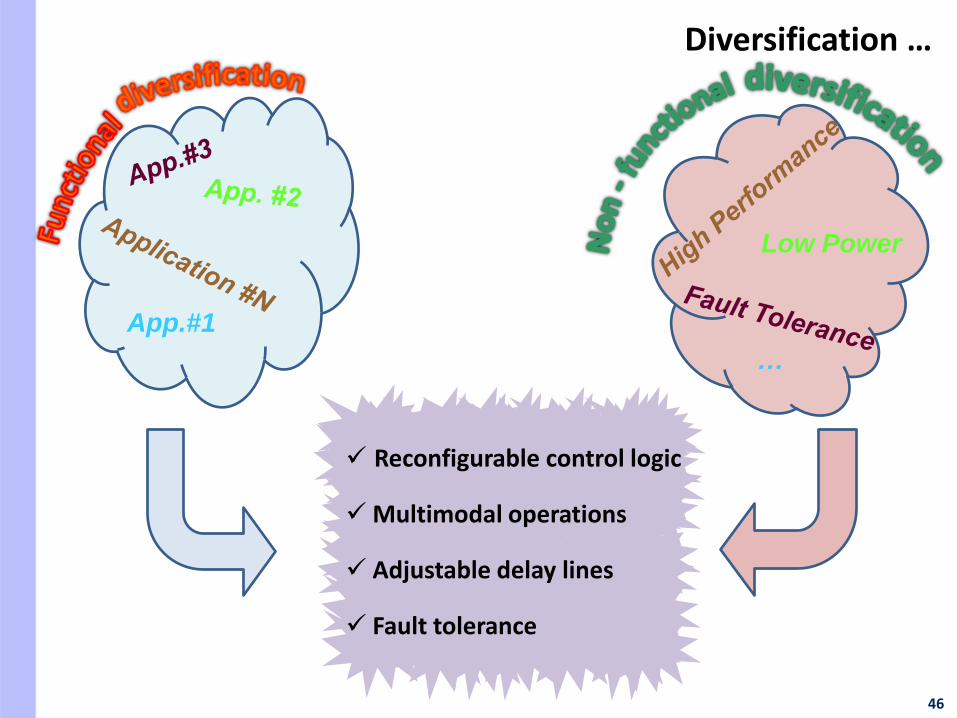
46

App.#1

Reconfigurable control logic

Multimodal operations

Adjustable delay lines

Fault tolerance

Low Power

…

Diversification …

47

Microprocessor architecture

48

Conceptual view of the design process

Design stages Implementation Intel 8051

49

WORKCRAFT FRAMEWORK

50

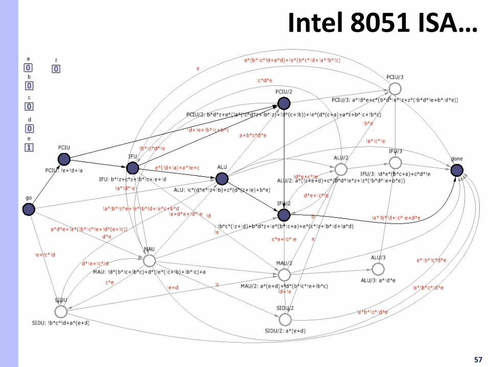
Intel 8051 ISA…

51

Intel 8051 ISA…

52

Intel 8051 ISA…

53

Intel 8051 ISA…

54

Intel 8051 ISA…

55

Intel 8051 ISA…

56

Intel 8051 ISA…

57

Intel 8051 ISA…

Fully asynchronous implementation (bundled data protocol)

– adjustable delay lines

58

Intel 8051 Datapath…

adder

multiplier

divider

adder

adder divider

High performance

Low Power

divider

multiplier

multiplier

Fault tolerance operation

DFT integration

59

Adaptable datapath unit

60

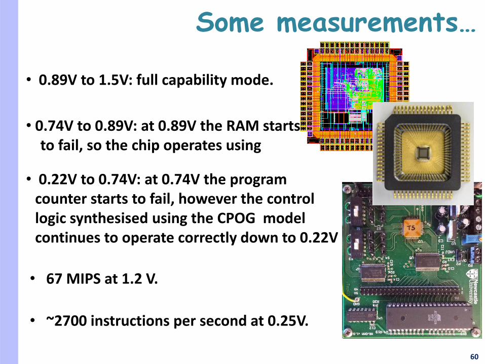
Some measurements…

• 0.22V to 0.74V: at 0.74V the program counter starts to fail, however the control logic synthesised using the CPOG model continues to operate correctly down to 0.22V

• 0.89V to 1.5V: full capability mode.

• 0.74V to 0.89V: at 0.89V the RAM starts to fail, so the chip operates using

• ~2700 instructions per second at 0.25V.

• 67 MIPS at 1.2 V.

Future of Real-Power Design

61

TODAY

62

Synthesis of asynchronous control DC-DC converters (A4A project)

Asynchronous control for Bucks

63

Asynchronous control for Bucks

64

Energy harvesting systems

Using Holistic project vision:

Sporadic source of energy does not allow for fancy power processing and therefore large storage

65

TODAY

Survival zone

66

Staying alive in variable, intermittent, low-power environments (Savvie Project)

Our View on EHA Systems

67

Asynchronous Control for Capacitor Banks

68

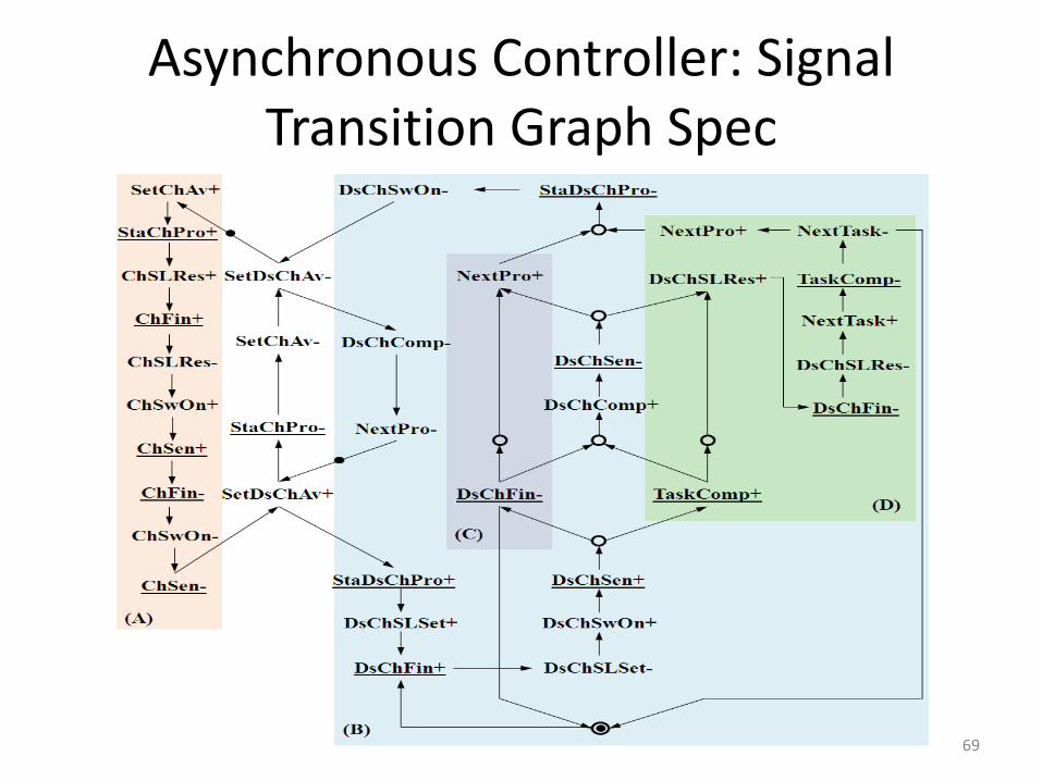
Asynchronous Controller: Signal Transition Graph Spec

69

Power-modulation and uncertainty • Localised prediction, from every moment at present

• Power has a certain profile (time trajectory) in the past and uncertain future

• Power-proportional and power-adaptive systems …

70

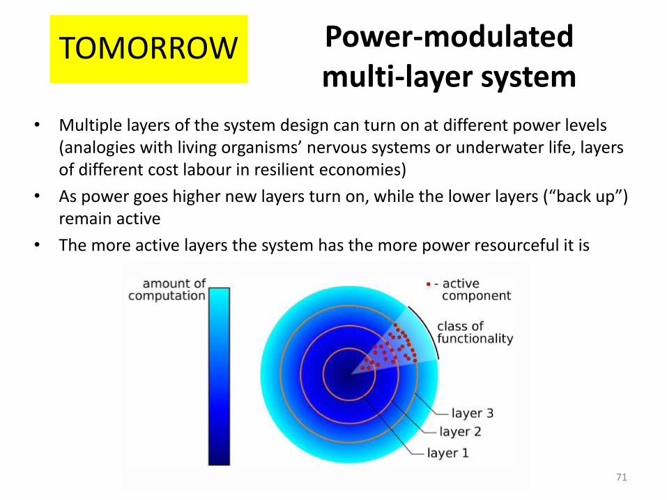
Power-modulated multi-layer system

• Multiple layers of the system design can turn on at different power levels (analogies with living organisms’ nervous systems or underwater life, layers of different cost labour in resilient economies)

• As power goes higher new layers turn on, while the lower layers (“back up”) remain active

• The more active layers the system has the more power resourceful it is

71

TOMORROW

Acknowledgements

• My colleagues at Newcastle and outside: Andrey Mokhov, Danil Sokolov, Fei Xia, Delong Shang, Maxim Rykunov, Reza Ramezani, Alex Kushnerov (Ben Gurion Uni), Bernard Stark (Bristol Uni) and many others – see http://async.org.uk

• EPSRC support: Dream Fellowship, projects: Holistic, PRiME, Power-Prop, Savvie, A4A

• Industrial support: ARM CASE studentship, Dialog Semiconductor

72

THANK YOU!

73