1 Algebra of Parameterised Graphs · 1 Algebra of Parameterised Graphs Andrey Mokhov, School of...

1

Algebra of Parameterised Graphs

Andrey Mokhov, School of Electrical and Electronic Engineering, Newcastle University, UKVictor Khomenko, School of Computing Science, Newcastle University, UK

One of the difficulties in designing modern hardware systems is the necessity to comprehend and to dealwith a very large number of system configurations, operational modes, and behavioural scenarios. It is ofteninfeasible to consider and specify each individual mode explicitly, and one needs methodologies and toolsto exploit similarities between the individual modes and work with groups of modes rather than individualones. The modes and groups of modes have to be managed in a compositional way: the specification of thesystem should be composed from specifications of its blocks. This includes both structural and behaviouralcomposition. Furthermore, one should be able to transform and optimise the specifications in a formal way.

In this paper we propose a new formalism, called Parameterised Graphs. It extends the existing Condi-tional Partial Order Graphs (CPOGs) formalism in several ways. First, it deals with general graphs ratherthan just partial orders. Moreover, it is fully compositional. To achieve this we introduce an algebra of Pa-rameterised Graphs by specifying the equivalence relation by a set of axioms, which is proved to be sound,minimal and complete. This allows one to manipulate the specifications as algebraic expressions using therules of this algebra. We demonstrate the usefulness of the developed formalism on several case studiescoming from the area of microelectronics design.

Categories and Subject Descriptors: G.2.2 [Mathematics of Computing]: Graph Theory

General Terms: Theory, Design, Synthesis

Additional Key Words and Phrases: Parameterised Graphs, Conditional Partial Order Graphs, SwitchingNetworks, Transistor Networks, Microelectronics, Instruction Set Architecture

1. INTRODUCTIONWhile the complexity of modern hardware exponentially increases due to Moore’s law,the time-to-market is reducing. The number of available transistors on chip exceedsthe capabilities of designers to meaningfully use them: this design productivity gap isa major challenge in the microelectronics industry [ITRS 2011]. One of the difficultiesof the design is the necessity to comprehend and to deal with a very large number ofsystem configurations, operational modes, and behavioural scenarios. The contempo-rary systems often have abundant functionality and enjoy features like fault-tolerance,dynamic reconfigurability, and power management, all of which greatly increase thenumber of possible modes of operation. Hence, it is often infeasible to consider andspecify each individual mode explicitly, and one needs methodologies and tools to ex-ploit similarities between the individual modes and work with groups of modes ratherthan individual ones. The modes and groups of modes have to be managed in a com-positional way: the specification of the system should be composed from specificationsof its blocks. This includes both structural and behavioural composition. Furthermore,one should be able to transform and optimise the specifications in a formal way.

A traditional way to achieve compositionality is to define an algebra. Many alge-bras have been proposed on various behavioural and structural models, e.g. composi-tions of graphs [Bauderon and Courcelle 1987; Eppstein 1992; Gadducci and Heckel1998], an algebra for network routing problems [Carre 1971], automata composi-tions [Gecseg 1974], Petri Net algebra [Best et al. 2001], algebra for delay-insensitivecircuits [Josephs and Udding 1993], and numerous process algebrae like CSP [Hoare1978], CCS [Milner 1982] and π-calculus [Milner et al. 1992]. The key difference ofour approach is the way it uses parameters to capture many variants of a system inone model. We build on the work started in [Mokhov and Yakovlev 2010], where aformal model, called Conditional Partial Order Graphs (CPOGs), was introduced. Itallowed to represent individual system configurations and operational modes as anno-

ACM Transactions on Embedded Computing Systems, Vol. 1, No. 1, Article 1, Publication date: January 2014.

1:2 A. Mokhov and V. Khomenko

tated graphs, and to overlay them exploiting their similarities. However, the formalismlacked the compositionality and the ability to compare and transform the specificationsin a formal way. In particular, CPOGs always represented the specification as a ‘flat’structure (similar to the canonical form defined in Section 2), hence a hierarchical rep-resentation of a system as a composition of its components was not possible. We extendthis formalism in several ways:

(1) We move from the graphs representing partial orders to general graphs. Neverthe-less, if partial orders are the most natural way to represent a certain aspect of asystem, this still can be handled.

(2) We handle both directed and undirected graphs.(3) The new formalism is fully compositional.(4) We describe the equivalence relation between the specifications as a set of axioms,

obtaining an algebra. This set of axioms is proved to be sound, minimal and com-plete.

(5) The developed formalism allows one to manipulate the specifications as algebraicexpressions using the rules of the algebra. In a sense this can be viewed as addinga syntactic level to the semantic representation of specifications, and is akin to therelationship between digital circuits and Boolean algebra.

The paper is organised as follows. In Section 2 we introduce directed ParameterisedGraphs and operations thereon. In Section 3 we generalise the developed theory byrepresenting it in the form of an algebra, where the properties of the graph opera-tions are formalised as axioms. In Section 4 we consider the transitive variant of thisalgebra, where the graphs are considered equal if their transitive closures coincide.This algebra is particularly suitable for modelling causal relationships. In Section 5we introduce the versions of these two algebrae for undirected graphs. In Section 6 wedemonstrate the usefulness of the developed formalisms on three case studies from thearea of microelectronics design:

(1) Development of a phase encoding controller, which represents information by theorder of arrival of signals on nwires. As there are n! possible arrival orders, there isa challenge to specify the set of corresponding behavioural scenarios in a compactway. The proposed formalism not only allows to solve this problem, but also doesit in a compositional way, by obtaining the final specification as a composition offixed-size fragments describing the behaviours of pairs of wires (the latter wasimpossible with CPOGs).

(2) Design of a microcontroller for a simple processor. The processor can execute sev-eral classes of instructions, and each class is characterised by a specific executionscenario of the operational units of the processor. In turn, the scenarios of con-ditional instructions have to be composed of sub-scenarios corresponding to thecurrent value of the appropriate ALU flag. The overall specification of the micro-controller is then obtained algebraically, by composing scenarios of each class ofinstructions.

(3) Synthesis of a NAND gate as a transistor network, demonstrating thus the appli-cation of an algebra of undirected graphs to switching networks.

2. PARAMETERISED GRAPHSA Parameterised Graph (PG) is a model which has evolved from Conditional PartialOrder Graphs (CPOG) [Mokhov and Yakovlev 2010]. We consider directed graphs G =(V,E) whose vertices are picked from the fixed alphabet of actions A = {a, b, ...}. Hencethe vertices of G would usually model actions (or events) of the system being designed,while the arcs would usually model the precedence or causality relation: if there is an


Algebra of Parameterised Graphs 1:3

a cb

(a) Graph G1

d

(b) Graph G2

a

d

cb

(c) Graph G1 +G2

a

d

cb

(d) Graph G1 → G2

Fig. 1: Overlay and sequence example (no common vertices)

d

ba

(a) Graph G1

d

cb

(b) Graph G2

a

d

cb

(c) Graph G1 +G2

a

d

cb

(d) Graph G1 → G2

Fig. 2: Overlay and sequence example (common vertices)

arc going from a to b then action a precedes action b. We will denote the empty graph(∅, ∅) by ε and the singleton graphs ({a}, ∅) simply by a, for any a ∈ A.

Let G1 = (V1, E1) and G2 = (V2, E2) be two graphs, where V1 and V2 as well as E1

and E2 are not necessarily disjoint. We define the following operations on graphs (inthe order of increasing precedence):

Overlay: G1 +G2df= (V1 ∪ V2, E1 ∪ E2).

Sequence: G1 → G2df= (V1 ∪ V2, E1 ∪ E2 ∪ V1 × V2).

Condition: [1]Gdf= G and [0]G

df= ε.

In other words, the overlay + and sequence→ are binary operations on graphs with thefollowing semantics: G1+G2 is a graph obtained by overlaying graphs G1 and G2, i.e. itcontains the union of their vertices and arcs, while graph G1 → G2 contains the unionplus the arcs connecting every vertex from graph G1 to every vertex from graph G2

(self-loops can be formed in this way if V1 and V2 are not disjoint). From the behaviouralpoint of view, if graphs G1 and G2 correspond to two systems then G1 +G2 correspondsto their parallel composition and G1 → G2 corresponds to their sequential composition.One can observe that any non-empty graph can be obtained by successively applyingthe operations + and→ to the singleton graphs: G =

∑(u,v)∈E u→ v.

Fig. 1 shows an example of two graphs together with their overlay and sequence.One can see that the overlay does not introduce any dependencies between the ac-tions coming from different graphs, therefore they can be executed concurrently. Onthe other hand, the sequence operation imposes the order on the actions by introduc-ing new dependencies between actions a, b and c coming from graph G1 and action dcoming from graph G2. Hence, the resulting system behaviour is interpreted as the be-haviour specified by graphG1 followed by the behaviour specified by graphG2. Anotherexample of system composition is shown in Fig. 2. Since the graphs have common ver-tices, their compositions are more complicated, in particular, their sequence containsthe self-dependencies (b, b) and (d, d) which lead to a deadlock in the resulting system:action a can occur, but all the remaining actions are locked.



Given a graph G, the unary condition operations can either preserve the graph (truecondition [1]G) or nullify it (false condition [0]G). They should be considered as a family{[b]}b∈B of operations parameterised by a Boolean value b.

Having defined the basic operations on the graphs, one can build graph expressionsusing these operations, the empty graph ε, the singleton graphs a ∈ A, and the Booleanconstants 0 and 1 (as the parameters of the conditional operations) — much like theusual arithmetical expressions. We now consider replacing the Boolean constants withBoolean variables or general predicates (this step is akin going from arithmetic toalgebraic expressions). The value of such an expression depends on the values of itsparameters, and so we call such an expression a parameterised graph (PG).

One can easily prove the following properties of the operations introduced above.

Properties of overlay:

• Identity:G+ ε = G

• Commutativity:G1 +G2 = G2 +G1

• Associativity:(G1 +G2) +G3 = G1 + (G2 +G3)

Properties of sequence:

• Left and right identity:ε→ G = GG→ ε = G

• Associativity:(G1 → G2)→ G3 = G1 → (G2 → G3)

Other properties:

• Left and right distributivity:G1 → (G2 +G3) = G1 → G2 +G1 → G3

(G1 +G2)→ G3 = G1 → G3 +G2 → G3

• Decomposition:

G1 → G2 → G3 = G1 → G2 +G1 → G3 +G2 → G3

Properties involving conditions:

• Conditional ε:[b]ε = ε

• Conditional overlay and sequence:[b](G1 +G2) = [b]G1 + [b]G2

[b](G1 → G2) = [b]G1 → [b]G2

• AND-condition and OR-condition:[b1 ∧ b2]G = [b1][b2]G[b1 ∨ b2]G = [b1]G+ [b2]G

• Condition regularisation:

[b1]G1 → [b2]G2 = [b1]G1 + [b2]G2 + [b1 ∧ b2](G1 → G2)



Now, due to the above properties of the operators, it is possible to define the followingcanonical form of a PG. In the proof below, we call a singleton graph, possibly prefixedwith a condition, a literal.

PROPOSITION 2.1 (CANONICAL FORM OF A PG). Any PG can be rewritten in thefollowing canonical form:(∑

v∈V[bv]v

)+

∑u,v∈V

[buv](u→ v)

, (1)

where:

(1) V is a subset of singleton graphs that appear in the original PG;(2) for all v ∈ V , bv are canonical forms of Boolean expressions and are distinct from 0;(3) for all u, v ∈ V , buv are canonical forms of Boolean expressions such that buv⇒bu∧bv.

PROOF. (i) First we prove that any PG can be converted to the form (1).All the occurrences of ε in the expression can be eliminated by the identity and con-

ditional ε properties (unless the whole PG equals to ε, in which case we take V = ∅). Toavoid unconditional subexpressions, we prefix the resulting expression with ‘[1]’, andthen by the conditional overlay/sequence properties we propagate all the conditionsthat appear in the expression down to the singleton graphs (compound conditions canbe always reduced to a single one by the AND-condition property). By the decompo-sition and distributivity properties, the expression can be rewritten as an overlay ofliterals and subexpressions of the form l1 → l2, where l1 and l2 are literals. The lattersubexpressions can be rewritten using the condition regularisation rule:

[b1]u→ [b2]v = [b1]u+ [b2]v + [b1 ∧ b2](u→ v)

Now, literals corresponding to the same singleton graphs, as well as subexpressionsof the form [b](u → v) that correspond to the same pair of singleton graphs u andv, are combined using the OR-condition property. Then the literals prefixed with 0conditions can be dropped. Now the set V consists of all the singleton graphs occurringin the literals. To turn the overall expression into the required form it only remainsto add missing subexpressions of the form [0](u → v) for every u, v ∈ V such that theexpression does not contain the subexpression of the form [b](u → v). Note that theproperty buv ⇒ bu ∧ bv is always enforced by this construction:

• condition regularisation ensures this property;• combining literals using the OR-condition property can only strengthen the righthand side of this implication, and so cannot violate it;• adding [0](u→ v) does not violate the property as it trivially holds when buv = 0.

(ii) We now show that (1) is a canonical form, i.e. if L = R then their canonical formscan(L) and can(R) coincide.

For the sake of contradiction, assume this is not the case. Then we consider twocases (all possible cases are symmetric to one of these two):

(1) can(L) contains a literal [bv]v whereas can(R) either contains a literal [b′v]v withb′v 6≡ bv or does not contain any literal corresponding to v, in which case we say thatit contains a literal [b′v]v with b′v = 0. Then for some values of parameters one of thegraphs will contain vertex v while the other will not.

(2) can(L) and can(R) have the same set V of vertices, but can(L) contains a subex-pression [buv](u → v) whereas can(R) contains a subexpression [b′uv](u → v) withb′uv 6≡ buv. Then for some values of parameters one of the graphs will contain the



arc (u, v) (note that due to buv ⇒ bu ∧ bv and b′uv ⇒ bu ∧ bv vertices u and v arepresent), while the other will not.

In both cases there is a contradiction with L = R.

This canonical form allows one to lift the notion of adjacency matrix of a graph to PGs.Recall that the adjacency matrix (buv) of a graph (V,E) is a |V | × |V | Boolean matrixsuch that buv = 1 if (u, v) ∈ E and buv = 0 otherwise. The adjacency matrix of a PGis obtained from the canonical form (1) by gathering the predicates buv into a matrix.The adjacency matrix of a PG is similar to that of a graph, but it contains predicatesrather than Boolean values. It does not uniquely determine a PG, as the predicatesof the vertices cannot be derived from it; to fully specify a PG one also has to providepredicates bv from the canonical form (1).

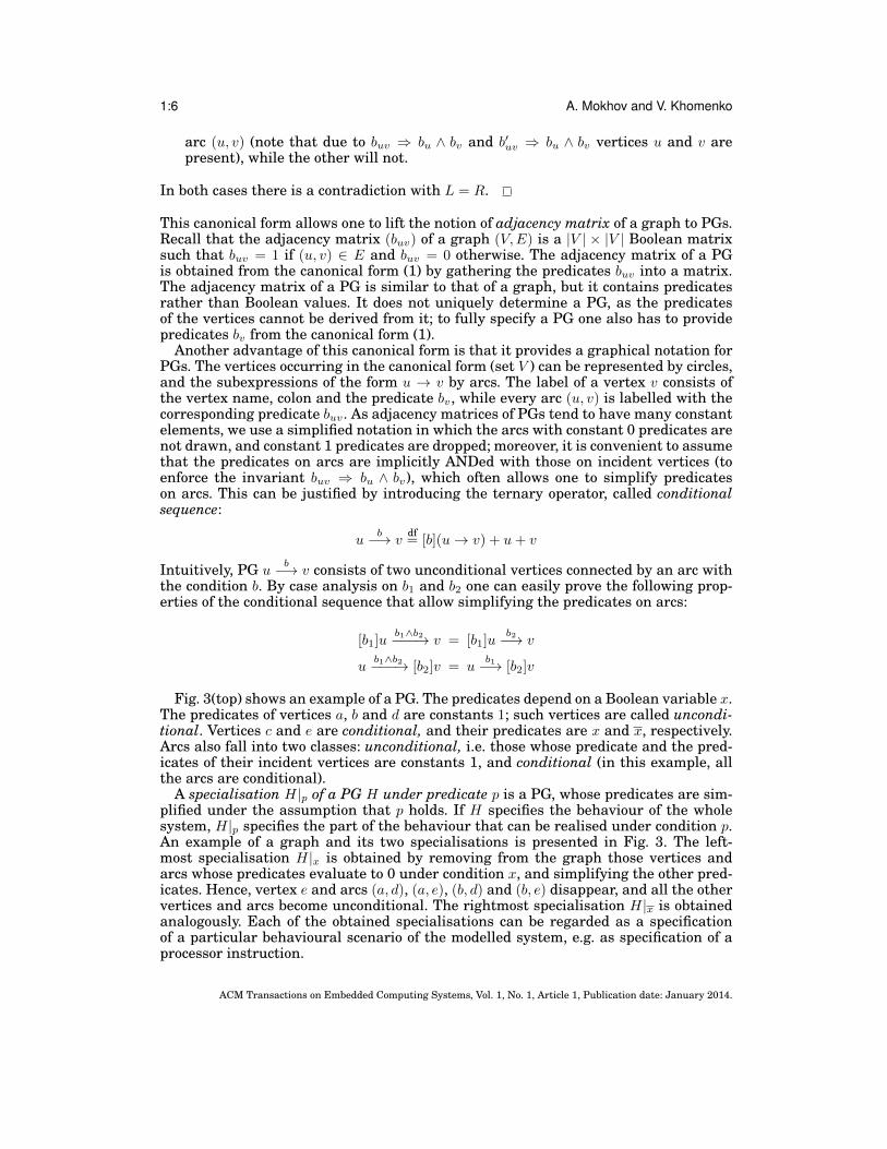
Another advantage of this canonical form is that it provides a graphical notation forPGs. The vertices occurring in the canonical form (set V ) can be represented by circles,and the subexpressions of the form u → v by arcs. The label of a vertex v consists ofthe vertex name, colon and the predicate bv, while every arc (u, v) is labelled with thecorresponding predicate buv. As adjacency matrices of PGs tend to have many constantelements, we use a simplified notation in which the arcs with constant 0 predicates arenot drawn, and constant 1 predicates are dropped; moreover, it is convenient to assumethat the predicates on arcs are implicitly ANDed with those on incident vertices (toenforce the invariant buv ⇒ bu ∧ bv), which often allows one to simplify predicateson arcs. This can be justified by introducing the ternary operator, called conditionalsequence:

ub−→ v

df= [b](u→ v) + u+ v

Intuitively, PG ub−→ v consists of two unconditional vertices connected by an arc with

the condition b. By case analysis on b1 and b2 one can easily prove the following prop-erties of the conditional sequence that allow simplifying the predicates on arcs:

[b1]ub1∧b2−−−→ v = [b1]u

b2−→ v

ub1∧b2−−−→ [b2]v = u

b1−→ [b2]v

Fig. 3(top) shows an example of a PG. The predicates depend on a Boolean variable x.The predicates of vertices a, b and d are constants 1; such vertices are called uncondi-tional. Vertices c and e are conditional, and their predicates are x and x, respectively.Arcs also fall into two classes: unconditional, i.e. those whose predicate and the pred-icates of their incident vertices are constants 1, and conditional (in this example, allthe arcs are conditional).

A specialisation H|p of a PG H under predicate p is a PG, whose predicates are sim-plified under the assumption that p holds. If H specifies the behaviour of the wholesystem, H|p specifies the part of the behaviour that can be realised under condition p.An example of a graph and its two specialisations is presented in Fig. 3. The left-most specialisation H|x is obtained by removing from the graph those vertices andarcs whose predicates evaluate to 0 under condition x, and simplifying the other pred-icates. Hence, vertex e and arcs (a, d), (a, e), (b, d) and (b, e) disappear, and all the othervertices and arcs become unconditional. The rightmost specialisation H|x is obtainedanalogously. Each of the obtained specialisations can be regarded as a specificationof a particular behavioural scenario of the modelled system, e.g. as specification of aprocessor instruction.



a

d

b

c: x e: x_

a

d

b

c

a

d

b

e

x _

x _

x x_

Fig. 3: PG specialisations: H|x and H|x

2.1. Specification and composition of instructionsConsider a processing unit that has two registers, A and B, and can perform two dif-ferent instructions: addition and exchange of two variables stored in memory. The pro-cessor contains five datapath components (denoted by a . . . e) that can perform the fol-lowing atomic actions:

a) Load register A from memory;b) Load register B from memory;c) Compute the sum of the numbers stored in registers A and B, and store it in A;d) Save register A into memory;e) Save register B into memory.

Table I describes the addition and exchange instructions in terms of usage of theseatomic actions.

The addition instruction consists of loading the two operands from memory (causallyindependent actions a and b), their addition (action c), and saving the result (action d).Let us assume for simplicity that in this example all causally independent actions arealways performed concurrently, see the corresponding scenario ADD in the table.

The operation of exchange consists of loading the operands (causally independentactions a and b), and saving them into swapped memory locations (causally indepen-dent actions d and e), as captured by the XCHG scenario. Note that in order to startsaving one of the registers it is necessary to wait until both of them have been loadedto avoid overwriting one of the values.

One can see that the two scenarios in Table I appear to be the two specialisationsof the PG shown in Fig. 3, thus this PG can be considered as a joint specification ofboth instructions. Two important characteristics of such a specification are that thecommon events {a, b, d} are overlaid, and the choice between the two operations ismodelled by the Boolean predicates associated with the vertices and arcs of the PG. Asa result, in our model there is no need for a ‘nodal point’ of choice, which tend to appear



Instruction Addition Exchangea) Load A a) Load A

Action b) Load B b) Load Bsequence c) Add B to A d) Save A

d) Save A e) Save B

Execution

a

d

b

c

a

d

b

e

scenariowith maximum

concurrency

ADD XCHG

Table I: Two instructions specified as partial orders

in alternative specification models: a Petri Net (resp. Finite State Machine) wouldhave an explicit choice place (resp. state), and a specification written in a HardwareDescription Language would describe the two instructions by two separate branchesof a conditional statement if or case [de Micheli 1994].

The PG operations introduced above allow for a natural specification of the systemas a collection of its behavioural scenarios, which can share some common parts. Forexample, in this case the overall system is composed as

H = [x]ADD + [x]XCHG = [x]((a+ b)→ c+ c→ d) + [x]((a+ b)→ (d+ e)). (2)

Such specifications can often be simplified using the properties of graph operations.The next section describes the equivalence relation between the PGs with a set ofaxioms, thus obtaining an algebra.

3. ALGEBRA OF PARAMETERISED GRAPHSIn this section we define the algebra of parameterised graphs (PG-algebra).

PG-algebra is a tuple 〈G,+,→, [0], [1]〉, where G is a set of graphs whose vertices arepicked from the alphabet A and the operations parallel those defined for graphs above.The equivalence relation is given by the following axioms:

• + is commutative and associative• → is associative• ε is a left and right identity of→• → distributes over +:

p→ (q + r) = p→ q + p→ r(p+ q)→ r = p→ r + q → r

• Decomposition:

p→ q → r = p→ q + p→ r + q → r

• Condition: [0]p = ε and [1]p = p



The following derived equalities can be proved from PG-algebra axioms [Mokhovet al. 2011, Prop. 2, 3]:

• ε is an identity of +: p+ ε = p

• + is idempotent: p+ p = p

• Left and right absorption:

p+ p→ q = p→ qq + p→ q = p→ q

• Conditional ε: [b]ε = ε

• Conditional overlay and sequence:

[b](p+ q) = [b]p+ [b]q[b](p→ q) = [b]p→ [b]q

• AND-condition and OR-condition:[b1 ∧ b2]p = [b1][b2]p[b1 ∨ b2]p = [b1]p+ [b2]p

• Choice propagation:

[b](p→ q) + [b](p→ r) = p→ ([b]q + [b]r)[b](p→ r) + [b](q → r) = ([b]p+ [b]q)→ r

• Condition regularisation:

[b1]p→ [b2]q = [b1]p+ [b2]q + [b1 ∧ b2](p→ q)

Note that as ε is a left and right identity of→ and +, there can be no other identities forthese operations. Interestingly, unlike many other algebrae, the two main operationsin the PG-algebra have the same identity.

It is easy to see that PGs are a model of PG-algebra, as all the axioms of PG-algebraare satisfied by PGs; in particular, this means that PG-algebra is sound. Moreover,any PG-algebra expression has the canonical form (1), as the proof of Prop. 2.1 can bedirectly imported:

• It is always possible to translate a PG-algebra expression to this canonical form, aspart (i) of the proof relies only on the properties of PGs that correspond to eitherPG-algebra axioms or equalities above.

• If L = R holds in PG-algebra then L = R holds also for PGs (as PGs are a model ofPG-algebra), and so the PGs can(L) and can(R) coincide, see part (ii) of the proof.Since PGs can(L) and can(R) are in fact the same objects as the expressions can(L)and can(R) of the PG-algebra, (1) is a canonical form of a PG-algebra expression.

This also means that PG-algebra is complete w.r.t. PGs, i.e. any PG equality can beeither proved or disproved using the axioms of PG-algebra (by converting to the canon-ical form).

The provided set of axioms of PG-algebra is minimal, i.e. no axiom from this set canbe derived from the others. The minimality was checked by enumerating the fixed-sizemodels of PG-algebra with the help of the ALG tool [Bizjak and Bauer 2011]: It turnsout that removing any of the axioms leads to a different number of non-isomorphicmodels of a particular size, implying that all the axioms are necessary.

Hence, the following result holds:

THEOREM 3.1 (SOUNDNESS, MINIMALITY AND COMPLETENESS). The set of ax-ioms of PG-algebra is sound, minimal and complete w.r.t. PGs.



4. TRANSITIVE PARAMETERISED GRAPHS AND THEIR ALGEBRAIn many cases the arcs of the graphs are interpreted as the causality relation, and sothe graph itself is a partial order. However, in practice it is convenient to drop someor all of the transitive arcs, i.e. two graphs should be considered equal whenever theirtransitive closures are equal. E.g. in this case the graphs specified by the expressionsa → b + b → c and a → b + a → c + b → c are considered as equal. PGs with thisequality relation are called Transitive Parameterised Graphs (TPG). To capture thisalgebraically, we augment the PG-algebra with the Closure axiom:

if q 6= ε then p→ q + q → r = p→ q + p→ r + q → r.

One can see that by repeated application of this axiom one can obtain the transitiveclosure of any graph, including those with cycles. The resulting algebra is called Tran-sitive Parameterised Graphs Algebra (TPG-algebra).

Note that the condition q 6= ε in the Closure axiom is necessary, as otherwise

a+ b = a→ ε+ ε→ b = a→ ε+ a→ b+ ε→ b = a→ b,

and the operations + and→ become identical, which is clearly undesirable.The Closure axiom helps to simplify specifications by reducing the number of arcs

and/or simplifying their conditions. For example, consider the PG expression (2). As thescenarios of this PG are interpreted as the orders of execution of actions, it is naturalto use the Closure axiom. Note that the expression cannot be simplified in PG-algebra;however, in the TPG-algebra it can be considerably simplified:

[x]((a+ b)→ c+ c→ d) + [x]((a+ b)→ (d+ e)) = (closure)[x]((a+ b)→ c+ (a+ b)→ d+ c→ d) + [x]((a+ b)→ (d+ e)) = (decomposition)

[x]((a+ b)→ c→ d) + [x]((a+ b)→ (d+ e)) = (choice propagation)(a+ b)→ ([x](c→ d) + [x](d+ e)) = (conditional overlay)

(a+ b)→ ([x](c→ d) + [x]d+ [x]e) = (→ −identity)(a+ b)→ ([x](c→ d) + [x](ε→ d) + [x]e) = (choice propagation)

(a+ b)→ (([x]c+ [x]ε)→ d+ [x]e) = (conditional ε, identity)(a+ b)→ ([x]c→ d+ [x]e).

The corresponding TPG is shown in Fig. 4. Note that it has fewer conditional ele-ments than the PG in Fig. 3; though the specialisations are now different, they havethe same transitive closures.

We now lift the canonical form (1) to TPGs and TPG-algebra. Note that the onlydifference is the last requirement.

PROPOSITION 4.1 (CANONICAL FORM OF A TPG). Any TPG can be rewritten in thefollowing canonical form:(∑

v∈V[bv]v

)+

∑u,v∈V

[buv](u→ v)

, (3)

where:

(1) V is a subset of singleton graphs that appear in the original TPG;(2) for all v ∈ V , bv are canonical forms of Boolean expressions and are distinct from 0;(3) for all u, v ∈ V , buv are canonical forms of Boolean expressions such that buv⇒bu∧bv;(4) for all u, v, w ∈ V , buv ∧ bvw ⇒ buw.



a

d

b

c: x e: x_

a

d

b

c

a

d

b

e

x x_

Fig. 4: The PG from Fig. 3 simplified using the Closure axiom, together with its spe-cialisations

PROOF. (i) First we prove that any TPG can be converted to the form (3).We can convert the expression into the canonical form (1), which satisfies the re-

quirements 1–3. Then we iteratively apply the following transformation, while pos-sible: If for some u, v, w ∈ V , buv ∧ bvw ⇒ buw does not hold (i.e. requirement 4is violated), we replace the subexpression [buw](u → w) with [bnewuw ](u → w) wherebnewuw

df= buw ∨ (buv ∧ bvw). Observe that after this the requirement 4 will hold for u, v and

w, and the requirement 3 remains satisfied, i.e. bnewuw ⇒ bu ∧ bw due to buv ⇒ bu ∧ bv,bvw ⇒ bv ∧ bw and buw ⇒ bu ∧ bw. Moreover, the resulting expression will be equivalentto the one before this transformation due to the following equality (see [Mokhov et al.2011] for the proof):

if v 6= ε then [buv](u→ v) + [bvw](v → w) == [buv](u→ v) + [bvw](v → w) + [buv ∧ bvw](u→ w).

This iterative process converges, as there can be only finitely many expressions ofthe form (3) (recall that we assume that the predicates within the conditional operatorsare always in some canonical form), and each iteration replaces some predicate buwwith a greater one bnewuw , in the sense that buv strictly subsumes bnewuw (i.e. buw ⇒ bnewuwand buw 6≡ bnewuw always hold), i.e. no predicate can be repeated during these iterations.

(ii) We now show that (3) is a canonical form, i.e. if L = R then their canonical formscan(L) and can(R) coincide.

For the sake of contradiction, assume this is not the case. Then we consider twocases (all possible cases are symmetric to one of these two).

(1) can(L) contains a literal [bv]v whereas can(R) either contains a literal [b′v]v withb′v 6= bv or does not contain any literal corresponding to v, in which case we say thatit contains a literal [b′v]v with b′v = 0. Then for some values of parameters one of thegraphs will contain vertex v while the other will not.



(2) can(L) and can(R) have the same set V of vertices, but can(L) contains a subexpres-sion [buv](u→ v) and can(R) contains a subexpression [b′uv](u→ v) with b′uv 6≡ buv.Then for some values of parameters one of the graphs will contain the arc (u, v)while the other will not. Since the transitive closures of the graphs must be thesame due to can(L) = L = R = can(R), the other graph must contain a patht1t2 . . . tn where u = t1, v = tn and n ≥ 3; w.l.o.g., we assume that t1t2 . . . tn is ashortest such path. Hence, the canonical form (1) would contain the subexpres-sions [btiti+1 ](ti → ti+1), i = 1 . . . n−1, and moreover

∧n−1i=1 btiti+1 6= 0 for the cho-

sen values of the parameters, and so∧n−1i=1 btiti+1

6≡ 0. But then the iterative pro-cess above would have added to the canonical form the missing subexpression[bt1t2 ∧ bt2t3 ](t1 → t3), as the corresponding predicates 6≡ 0. Hence, for the chosenvalues of the parameters, there is an arc (t1, t3), contradicting the assumption thatt1t2 . . . tn is a shortest path between u and v.

In both cases there is a contradiction with L = R.

The process of constructing the canonical form (3) of a TPG from the canonical form (1)of a PG corresponds to computing the transitive closure of the adjacency matrix. Asthe entries of this matrix are predicates rather than Boolean values, this has to bedone symbolically. This is always possible, as each entry of the resulting matrix canbe represented as a finite Boolean expression depending on the entries of the originalmatrix only.

By the same reasoning as in the previous section, we can conclude that the followingresult holds.

THEOREM 4.2 (SOUNDNESS, MINIMALITY AND COMPLETENESS). The set of ax-ioms of TPG-algebra is sound, minimal and complete w.r.t. TPGs.

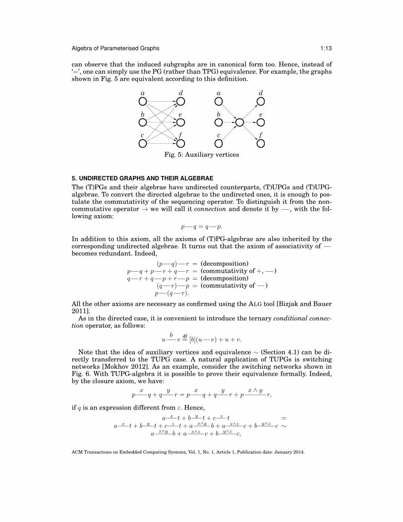
4.1. Auxiliary verticesIt is often convenient to use auxiliary vertices in TPGs. We do not name such verticesin our drawings, but they are assumed to have globally unique names. For example,Fig. 5 shows two TPGs representing the same connectivity between named vertices.Note that adding an unnamed intermediate vertex allows one to reduce the size of thegraph. Given a set of vertices S, η(S) will denote the subset of named vertices in S.

With auxiliary vertices the equivalence introduced in Section 3 needs to be amendedto take them into account.

Definition 4.3 (Equivalence with auxiliary vertices). Let p1 and p2 be two TPGswith the following canonical forms:

p1 =

(∑v∈V 1

[b1v]v

)+

∑u,v∈V 1

[b1uv](u→ v)

, p2 =

(∑v∈V 2

[b2v]v

)+

∑u,v∈V 2

[b2uv](u→ v)

.

Then they are equivalent, p1 ∼ p2, iff ∑v∈η(V 1)

[b1v]v

+

∑u,v∈η(V 1)

[b1uv](u→ v)

=

∑v∈η(V 2)

[b2v]v

+

∑u,v∈η(V 2)

[b2uv](u→ v)

.

In other words, two TPGs in canonical form are equivalent if their subgraphs inducedby named vertices coincide. Note that the above definition uses the ‘=’ relation on TPGsto compare the induced subgraphs, which in particular includes the Closure axiom.However, the original TPGs are in canonical form (and thus are ‘transitive’), and one



can observe that the induced subgraphs are in canonical form too. Hence, instead of‘=’, one can simply use the PG (rather than TPG) equivalence. For example, the graphsshown in Fig. 5 are equivalent according to this definition.

a

b

c

d

e

f

a

b

c

d

e

f

Fig. 5: Auxiliary vertices

5. UNDIRECTED GRAPHS AND THEIR ALGEBRAEThe (T)PGs and their algebrae have undirected counterparts, (T)UPGs and (T)UPG-algebrae. To convert the directed algebrae to the undirected ones, it is enough to pos-tulate the commutativity of the sequencing operator. To distinguish it from the non-commutative operator → we will call it connection and denote it by , with the fol-lowing axiom:

p q = q p.

In addition to this axiom, all the axioms of (T)PG-algebrae are also inherited by thecorresponding undirected algebrae. It turns out that the axiom of associativity ofbecomes redundant. Indeed,

(p q) r = (decomposition)p q + p r + q r = (commutativity of +, )q r + q p+ r p = (decomposition)

(q r) p = (commutativity of )p (q r).

All the other axioms are necessary as confirmed using the ALG tool [Bizjak and Bauer2011].

As in the directed case, it is convenient to introduce the ternary conditional connec-tion operator, as follows:

ubv

df= [b](u v) + u+ v.

Note that the idea of auxiliary vertices and equivalence ∼ (Section 4.1) can be di-rectly transferred to the TUPG case. A natural application of TUPGs is switchingnetworks [Mokhov 2012]. As an example, consider the switching networks shown inFig. 6. With TUPG-algebra it is possible to prove their equivalence formally. Indeed,by the closure axiom, we have:

pxq + q

yr = p

xq + q

yr + p

x ∧ yr,

if q is an expression different from ε. Hence,a x t+ b y t+ c z t =

a x t+ b y t+ c z t+ a x∧y b+ a x∧z c+ b y∧z c ∼a x∧y b+ a x∧z c+ b y∧z c,



where t denotes the auxiliary vertex.

a

b c

x

y z

a

b cy z

x zx y

Fig. 6: Two equivalent switching networks (the well-known ∆-Y transformation, seee.g. [Shannon 1938])

PROPOSITION 5.1 (CANONICAL FORM OF A (T)UPG). Any (T)UPG can be rewrit-ten in the following canonical form:(∑

v∈V[fv]v

)+

∑u,v∈Vu≤v

[fuv](u v)

,

where:

(1) V is a subset of singleton graphs that appear in the original (T)UPG, and ≤ is somearbitrary total order on the alphabet of vertices;

(2) for all v ∈ V , fv are canonical forms of Boolean expressions and are distinct from 0;(3) for all u, v ∈ V , u ≤ v, fuv are canonical forms of Boolean expressions such that

fuv ⇒ fu ∧ fv;(4) for the TUPG case only: for all u, v, w ∈ V , fuv ∧ fvw ⇒ fuw (the transitivity require-

ment); for convenience, we assume fuv = fvu.

PROOF SKETCH. By replacing every occurrence of the connection operator in theexpression by the sequence operator→ we obtain a PG. We then compute the canonicalform as explained in the proof of Prop. 2.1.

For TUPG, in the resulting PG we replace each occurrence of [fuv](u → v) with[fuv](u → v) + [fuv](v → u), and compute the transitive closure as described in theproof of Prop. 4.1.

Now we replace every occurrence of → with and combine terms [fuv](u v) and[fvu](v u) as follows:

[fuv](u v) + [fvu](v u) = (commutativity)[fuv](u v) + [fvu](u v) = (OR-condition)

[fuv ∨ fvu](u v).

Assuming u ≤ v, this guarantees that the resulting (T)UPG has at most one termcorresponding to any pair of nodes u and v. One can now show that requirements (1)-(4) are satisfied, as in the proofs of (T)PG cases.

By paralleling the reasoning for (T)PG-algebrae one can conclude that the followingresult holds.

THEOREM 5.2 (SOUNDNESS, MINIMALITY AND COMPLETENESS). The sets of ax-ioms of (T)UPG-algebrae are sound, minimal and complete w.r.t. (T)UPGs.



a

b

c

d

(a) Phase encoded data

Matrixphaseencoder

v1v2

vn

x12x21x13x31

x(n-1)nxn(n-1)

......

(b) Matrix phase encoder

Fig. 7: Multiple rail phase encoding

6. CASE STUDIESIn this section we consider several practical case studies from hardware synthesis.The advantage of graph algebrae is that they allow for a formal and compositionalapproach to system design. Moreover, using their rules one can formally manipulatespecifications, in particular, algebraically simplify them.

6.1. Phase encodersThis section demonstrates the application of PG-algebra to designing the multiple railphase encoding controllers [D’Alessandro et al. 2006]. They use several wires for com-munication, and data is encoded by the order of occurrence of transitions in the com-munication lines. Fig. 7(a) shows an example of a data packet transmission over a4-wire phase encoding communication channel. The order of rising signals on wiresindicates that permutation abdc is being transmitted. In total it is possible to trans-mit any of the n! different permutations over an n-wire channel in one communicationcycle. This makes the multiple rail phase encoding protocol very attractive for its in-formation efficiency [Mokhov and Yakovlev 2010].

Phase encoding controllers contain an exponential number of behavioural scenariosw.r.t. the number of wires, and are very difficult for specification and synthesis usingconventional approaches. In this section we apply PG-algebra to specification of ann-wire matrix phase encoder — a basic phase encoding controller that generates apermutation of signal events given a matrix representing the order of the events inthe permutation.

Fig. 7(b) shows the top-level view of the controller’s structure. Its inputs are(n2

)dual-

rail ports that specify the order of signals to be produced at the controller’s n outputwires. The inputs of the controller can be viewed as an n×n Boolean matrix (xij) withdiagonal elements being 0. The outputs of the controller will be modelled by n actionsvi ∈ A. Whenever xij = 1, event vi must happen before event vj . It is guaranteedthat xij and xji cannot be 1 at the same time, however, they can be simultaneously 0,meaning that the relative order of the events is not known yet and the controller hasto wait until xij = 1 or xji = 1 is satisfied (other outputs for which the order is alreadyknown can be generated meanwhile).

The overall specification of the controller is obtained as the overlay∑

1≤i<j≤n

Hij of fixed-

size expressions Hij modelling the behaviour of each pair of outputs. In turn, each Hij

is an overlay of three possible scenarios:

(1) If xij = 1 (and so xji = 0) then there is a causal dependency between vi and vj ,described using the PG-algebra sequence operator: vi → vj .

(2) If xji = 1 (and so xij = 0) then there is a causal dependency between vj and vi:vj → vi.



vi vjxji_

xij_

(a) Hij

v1

v2

v3x31_

x13_

x21_x12_

x32

_

x23

_

(b) H12 +H13 +H23

Fig. 8: PGs related to matrix phase encoder specification

(3) If xij = xji = 0 then neither vi nor vj can be produced yet; this is expressed by acircular wait condition between vi and vj : vi → vj + vj → vi.1

We prefix each of the scenarios with its precondition and overlay the results:

Hij = [xij ∧ xji](vi → vj) + [xji ∧ xij ](vj → vi)++[xij ∧ xji](vi → vj + vj → vi).

Using the rules of PG-algebra, we can simplify this expression to

[xji](vi → vj) + [xij ](vj → vi),

or, using the conditional sequence operator, to

[xij ∨ xji](vixji−→ vj + vj

xij−→ vi).

Now, bearing in mind that condition [xij ∨ xji] is assumed to hold in the propercontroller environment (xij and xji cannot be 1 simultaneously), we can replace itwith [1] and drop it. The resulting expression can be graphically represented as shownin Fig. 8(a). An example of an overall controller specification

∑1≤i<j≤n

Hij for the case when

n = 3 is shown in Fig. 8(b). The synthesis of this specification to a digital circuit can beperformed in a way similar to [Mokhov and Yakovlev 2010].

6.2. Processor microcontroller and instruction set designThis section demonstrates application of TPG-algebra to designing processor micro-controllers. Specification of such a complex system as a processor has to start at thearchitectural level, which helps to manage the system complexity by structural ab-straction [de Micheli 1994].

Fig. 9 shows the architecture of an example processor [MSP430 manual]. SeparateProgram memory and Data memory blocks are accessed via Instruction fetch (IFU) andMemory access (MAU) units, respectively. The other two operational units are: Arith-metic logic unit (ALU) and Program counter increment unit (PCIU). The units are con-trolled using request-acknowledgement interfaces (depicted as bidirectional arrows)by Central microcontroller, which is our primary design objective.

The processor has four registers: two general purpose registers A and B, Programcounter (PC) storing the address of the current instruction in the program memory,and Instruction register (IR) storing the opcode (operation code) of the current instruc-tion. For the purpose of this paper, the actual width of the registers (the number ofbits they can store) is not important. ALU has access to all the registers via the reg-ister bus; MAU has access to general purpose registers only; IFU, given the address

1There are other ways to describe this scenario, e.g. by creating self-loops vi → vi + vj → vj .



Programbcounterb(PC)

Instructionbregisterb(IR)

Programmemory

RegisterbAb(accumulator)

RegisterbBb(address)

Instructionfetch

unitb(IFU)

Centralmicrocontroller

opcode

PCincrement

unitb(PCIU)

Memoryaccess

unitb(MAU)

Datamemory

registerbbus

go

done

executionbcontrol

Arithmeticlogicbunitb(ALU)

flags

Fig. 9: Architecture of an example processor

of the next instruction in PC, reads its opcode into IR; and PCIU is responsible for in-crementing PC (moving to the next instruction). The microcontroller has access to IRand ALU flags (information about the current state of ALU which is used in branchinginstructions).

Now we define the set of instructions of the processor. Rather than listing all theinstructions, we describe classes of instructions with the same addressing mode andthe same execution scenario. As the scenarios here are partial orders of actions, we useTPG-algebra, and the corresponding TPGs are shown in Fig. 10.

ALU operation Rn to Rn An instruction from this class takes two operandsstored in the general purpose registers (A and B), performs an operation, and writesthe result back into one of the registers (so called register direct addressing mode).Examples: ADD A, B – addition A := A + B; MOV B , A – assignment B := A.ALU works concurrently with PCIU and IFU, which is captured by the expressionALU +PCIU → IFU ; the corresponding PG is shown in Fig. 10(a). As soon as both con-current branches are completed, the processor is ready to execute the next instruction.Note that it is not important for the microcontroller which particular ALU operationis being executed (ADD , MOV , or any other instruction from this class) because thescenario is the same from its point of view (it is the responsibility of ALU to detectwhich operation it has to perform according to the current opcode).

ALU operation #123 to Rn In this class of instructions one of the operands is aregister and the other is a constant which is given immediately after the instructionopcode (e.g. SUB A, #5 – subtraction A := A − 5), so called immediate addressingmode. At first, the constant has to be fetched into IR, modelled as PCIU → IFU .Then ALU is executed concurrently with another increment of PC: ALU + PCIU ′ (weuse ′ to distinguish the different occurrences of actions of the same unit). Finally, itis possible to fetch the next instruction into IR: IFU ′. The overall scenario is thenPCIU → IFU → (ALU + PCIU ′)→ IFU ′.

ALU operation Rn to PC This class contains operations for unconditionalbranching, in which PC register is modified. Branching can be absolute or relative:MOV PC , A — absolute branch to address stored in register A, PC := A; ADD PC , B



ALU

PCIU IFU

(a) ALU op. Rn to Rn

PCIU

ALU

IFU

PCIU'

IFU'

(b) ALU op. #123 to Rn

ALU IFU

(c) ALU op. Rn to PC

PCIU IFU'IFU ALU

(d) ALU op. #123 to PC

MAU

PCIU IFU

(e) Memory access

ALU

IFUPCIU

ALU': lt

(f) Cond. ALU op. Rn to Rn

ALU

IFU: lt

IFU'PCIU'PCIU

ALU': lt

(g) Cond. ALU op. #123 to Rn

IFU: lt

IFU'PCIU

ALU

ALU': lt

PCIU': lt_

(h) Cond. ALU op. #123 to PC

Fig. 10: TPG specifications of instruction classes

— relative branch to the address B instructions ahead of the current address, PC :=PC +B. The scenario is very simple in this case: ALU → IFU .

ALU operation #123 to PC Instructions in this class are similar to those above,with the exception that the branch address or offset is specified explicitly as a constant.The execution scenario is composed of: PCIU → IFU (to fetch the constant), followedby an ALU operation, and finally by another IFU operation, IFU ′. Hence, the overallscenario is PCIU → IFU → ALU → IFU ′.

Memory access There are two instructions in this class: MOV A, [B ] andMOV [B ], A. They load/save register A from/to memory location with address stored inregister B. Due to the presence of separate program and data memory access blocks,this memory access can be performed concurrently with the next instruction fetch:PCIU → IFU + MAU .

Conditional instructions These three classes of instructions are similar to theirunconditional versions above, with the difference that they are performed only if thecondition A < B holds. The first ALU action compares registers A and B, setting theALU flag lt (less than) according to the result of the comparison. This flag is thenchecked by the microcontroller in order to decide on the further scheduling of actions.

Rn to Rn This instruction conditionally performs an ALU operation with the reg-isters (if the condition does not hold, the instruction has no effect, except changingthe ALU flags). The operation starts with an ALU operation comparing A with B; de-pending on the result of this comparison, i.e. the status of the flag lt, the second ALUoperation may be performed. This is captured by the expression ALU → [lt]ALU ′. Con-currently with this, the next instruction is fetched: PCIU → IFU . Hence, the overallscenario is PCIU → IFU + ALU → [lt]ALU ′.

#123 to Rn This instruction conditionally performs an ALU operation with a reg-ister and a constant which is given immediately after the instruction opcode (if thecondition does not hold, the instruction has no effect, except changing the ALU flags).We consider the two possible scenarios:



Instructions class Opcode: xyzALU Rn to Rn 000

ALU #123 to Rn 110ALU Rn to PC 101

ALU #123 to PC 010Memory access 100

C/ALU Rn to Rn 001C/ALU #123 to Rn 111C/ALU #123 to PC 011

MAU: d

PCIU: g

b

e

PCIU': (x+f) y

ALU: d

IFU': y

IFU: f_

y

_

z

ALU': z c g_. .

.

a = x+y g = e+y_

b = z a_. d = y b

_.e = a b

_.

f = y c.c = b lt

_._

Fig. 11: Optimal 3-bit instruction opcodes and the corresponding TPG specification ofthe microcontroller

(1) A < B holds: First, ALU compares A and B concurrently with a PC increment;sinceA < B holds, the ALU sets flag lt and the constant is fetched to the instructionregister: (ALU +PCIU )→ IFU . After that PC has to be incremented again, PCIU ′,and ALU performs the operation, ALU ′. Finally, the next instruction is fetched (itcannot be fetched concurrently with ALU ′ as ALU is using the constant in IR):(ALU ′ + PCIU ′)→ IFU ′.

(2) A < B does not hold: First, ALU compares A and B concurrently with a PC in-crement; since A < B does not hold, the ALU resets flag lt and the constant thatfollows the instruction opcode is skipped by incrementing the PC: (ALU +PCIU )→PCIU ′. Finally, the next instruction is fetched: IFU ′.

Hence, the overall scenario is the overlay of the two subscenarios above prefixed withappropriate conditions (here we denote the predicate A < B by lt):[lt]((ALU+PCIU )→IFU→(ALU ′+PCIU ′)→IFU ′)+[lt]((ALU+PCIU )→PCIU ′→IFU ′).

This expression can be simplified using the rules of TPG-algebra:2

(ALU + PCIU )→ [lt]IFU → (PCIU ′ + [lt]ALU ′)→ IFU ′.

#123 to PC This instruction performs a conditional branching in which the branchaddress or offset is specified explicitly as a constant. We consider the two possiblescenarios:

(1) A < B holds: First, ALU compares A and B concurrently with a PC increment;sinceA < B holds, the ALU sets flag lt and the constant is fetched to the instructionregister: (ALU +PCIU )→ IFU . After that ALU performs the branching operationby modifying PC, ALU ′. After PC is changed, the next instruction is fetched, IFU ′.

(2) A < B does not hold: the scenario is exactly the same as in the #123 to Rn casewhen A < B does not hold.

Hence, the overall scenario is the overlay of the two subscenarios above prefixed withappropriate conditions (here we denote the predicate A < B by lt):

[lt]((ALU+PCIU )→IFU→ALU ′→IFU ′)+[lt]((ALU+PCIU )→PCIU ′→IFU ′).

2This case illustrates the advantage of using the new hierarchical approach that allows to specify the sys-tem as a composition of scenarios and formally manipulate them in an algebraic fashion. In the previouspaper [Mokhov et al. 2011] the CPOG for this class of instruction was designed monolithically, and becauseof this the arc between ALU ′ and IFU ′ was missed. Adding this arc not only fixes the dangerous race be-tween these two blocks, but also leads to a smaller microcontroller due to the additional similarity betweenTPGs for this class of instructions and for the one described below.



c

(a) >+c ⊥

c

(b) > c+⊥

c

(c) c a∧b ⊥+ c a∧b >

c

(d) c a t+ t b ⊥+ c a >+ c b >

Fig. 12: Synthesis of a switching network implementing functionality of a NAND gate

This expression can be simplified using the rules of TPG-algebra:

(ALU + PCIU )→ ([lt]PCIU ′ + [lt](IFU → ALU ′))→ IFU ′.

The overall specification of the microcontroller can now be obtained by prefixing thescenarios with appropriate conditions and overlaying them. These conditions can benaturally derived from the instruction opcodes. The opcodes can be either imposedexternally or chosen with the view to optimise the microcontroller. In the latter case,TPG-algebra and TPGs allow for a formal statement of this optimisation problem andaid in its solving; in particular, the sizes of the TPG-algebra expression or TPG areuseful measures of microcontroller complexity (there is a compositional translationfrom a TPG-algebra expression into a linear-size circuit). In this paper we do not gointo details of how to select the optimal encoding, but see [Mokhov et al. 2011]. Wejust note that it is natural to use three bits for opcodes as there are eight classes ofinstructions, and give an example of optimal 3-bit encoding in the table in Fig. 11; theTPG specification of the corresponding microcontroller is shown in the right part ofthis figure (the TPG-algebra expression is not shown because of its size).

6.3. NAND gate in CMOS technologyThis section demonstrates application of TUPG-algebra to switching networks, on theexample of synthesising a NAND gate as a transistor network. Given two input signalsa and b, the transistor network produces the output signal c connected to the ground(represented by the special vertex ⊥) if the condition a ∧ b holds, and to the powersupply (the special vertex >) otherwise. The networks implementing functionality ofthese two scenarios are shown in Figs. 12(a,b). Overlaying them with the appropriateconditions, we obtain the following TUPG expression:

NAND = [a ∧ b](>+ c ⊥) + [a ∧ b](> c+⊥).

Simplifying this expression yields:

NAND = ca ∧ b ⊥+ c

a ∧ b >.

The corresponding switching network is shown in Fig. 12(c). Since in the CMOS tech-nology each switch can be controlled only by one signal (positive literals correspondto n-type transistors, and negative ones correspond to p-type transistors), we have torefine the result by splitting the switches into simpler ones. This requires an additionof a new auxiliary node t:

NAND ∼ c at+ t

b ⊥+ ca >+ c

b >.



Fig. 12(d) shows the final circuit, which matches the standard NAND gate imple-mentation in the CMOS technology. (In general, this approach is not restricted tocomplementary-symmetric transistor networks as in CMOS.)

7. CONCLUSIONSWe introduced a new formalism called Parameterised Graphs and the correspondingalgebra. The formalism allows one to manage a large number of system configurationsand execution scenarios, exploit similarities between them to simplify the specifica-tion, and to work with groups of configurations and modes rather than with individualones. The modes and groups of modes can be managed in a compositional way, andthe specifications can be manipulated (transformed and/or optimised) algebraically ina fully formal and natural way.

We develop two variants of the algebra of parameterised graphs, corresponding tothe two natural graph equivalences: graph isomorphism and isomorphism of transitiveclosures. We also introduce the undirected versions of these algebrae. All four casesare specified axiomatically, and the soundness, minimality and completeness of theresulting sets of axioms are formally proved. Moreover, the canonical forms of algebraicterms are developed in each case.

The usefulness of the developed formalism has been demonstrated on several casestudies: i) a phase encoding controller, ii) a processor microcontroller, and iii) synthe-sis of a CMOS switching network. The formalism allows one to capture all the execu-tion scenarios in these examples algebraically, by composing individual scenarios andgroups of scenarios. The possibility of algebraic manipulation is essential to obtain theoptimised final specification in each case.

The developed formalism is also convenient for implementation in a tool, as manipu-lating algebraic terms is much easier than general graph manipulation; in particular,the theory of term rewriting can be naturally applied to derive the canonical forms.

In future work we plan to automate the algebraic manipulation of PGs, and imple-ment automatic synthesis of PGs into digital circuits. For the latter, much of the codedeveloped for the precursor formalism of Conditional Partial Order Graphs (CPOGs)can be re-used. One of the important problems that needs to be automated is that ofsimplification of (T)PG expressions, in the sense of deriving an equivalent expressionwith the minimum possible number of operators. Our preliminary research suggeststhat this problem is strongly related to modular decomposition of graphs [McConnelland de Montgolfier 2005].

Acknowledgements The authors would like to thank Arseniy Alekseyev, AshurRafiev, and Alex Yakovlev for their help in preparation of the previous versions of thiswork. This research was supported by the EPSRC grants EP/I038357/1 (eFuturesXD,project POWERPROP) and EP/K001698/1 (UNCOVER).

REFERENCESM. Bauderon and B. Courcelle. 1987. Graph expressions and graph rewritings. Mathematical Systems Theory

20, 1 (1987), 83–127.E. Best, R. Devillers, and M. Koutny. 2001. Petri Net Algebra. Springer.A. Bizjak and A. Bauer. Faculty of Mathematics and Physics, University of Ljubljana, 2011. ALG User Man-

ual.B.A. Carre. 1971. An algebra for network routing problems. IMA Journal of Applied Mathematics 7, 3 (1971),

273–294.C. D’Alessandro, D. Shang, A. Bystrov, A. Yakovlev, and O. Maevsky. 2006. Multiple-Rail Phase-Encoding

for NoC. In Proc. of International Symposium on Advanced Research in Asynchronous Circuits andSystems (ASYNC). 107–116.

G. de Micheli. 1994. Synthesis and Optimization of Digital Circuits. McGraw-Hill Higher Education.



D. Eppstein. 1992. Parallel recognition of series-parallel graphs. Information and Computation 98, 1 (1992),41–55.

F. Gadducci and R. Heckel. 1998. An inductive view of graph transformation. In Recent Trends in AlgebraicDevelopment Techniques. Springer, 223–237.

F. Gecseg. 1974. Composition of automata. In Automata, Languages and Programming. Springer, 351–363.C.A.R. Hoare. 1978. Communicating sequential processes. Commun. ACM 21, 8 (1978), 666–677.ITRS 2011. International Technology Roadmap for Semiconductors: Design. (2011). URL: http://www.itrs.

net/Links/2011ITRS/2011Chapters/2011Design.pdf.M.B. Josephs and J.T. Udding. 1993. An overview of DI algebra. In Proceeding of the Twenty-Sixth Hawaii

International Conference on System Sciences, Vol. 1. 329–338.R. McConnell and F. de Montgolfier. 2005. Linear-time modular decomposition of directed graphs. Discrete

Applied Mathematics 145, 2 (2005), 198–209.R. Milner. 1982. A calculus of communicating systems. Springer.R. Milner, J. Parrow, and D. Walker. 1992. A Calculus of Mobile Processes, Part I. Information and compu-

tation 100, 1 (1992), 1–40.A. Mokhov. 2012. An Algebra of Switching Networks. Technical Report NCL-EEE-MSD-TR-2012-178. New-

castle University.A. Mokhov, A. Alekseyev, and A. Yakovlev. 2011. Encoding of processor instruction sets with explicit concur-

rency control. IET Computers and Digital Techniques 5, 6 (2011), 427–439.A. Mokhov, V. Khomenko, A. Alekseyev, and A. Yakovlev. 2011. Algebra of Parametrised Graphs. Technical

Report CS-TR-1307. School of Computing Science, Newcastle University. URL: http://www.cs.ncl.ac.uk/publications/trs/papers/1307.pdf.

A. Mokhov and A. Yakovlev. 2010. Conditional Partial Order Graphs: Model, Synthesis and Application.IEEE Trans. Comput. 59, 11 (2010), 1480–1493.

MSP430x4xx. MSP430x4xx Family User’s Guide. http://www.ti.com/lit/ug/slau056l/slau056l.pdfC. E. Shannon. 1938. A Symbolic Analysis of Relay and Switching Circuits. Transactions of the American

Institute of Electrical Engineers 57 (1938), 713–723.


1 Algebra of Parameterised Graphs · 1 Algebra of Parameterised Graphs Andrey Mokhov, School of...

Documents

Transcript of 1 Algebra of Parameterised Graphs · 1 Algebra of Parameterised Graphs Andrey Mokhov, School of...