Airside Economizer Low Limit Effect on Energy and Thermal ...

Airside Economizer Low Limit Effect on Energy and Thermal Comfort

By

Copyright 2015

Samantha Bakke

Submitted to the graduate degree program in Civil, Environmental and Architectural

Engineering Department and the Graduate Faculty of the University of Kansas in partial

fulfillment of the requirements for the degree of Master of Science in Architectural

Engineering.

________________________________

Chairperson Brian A. Rock

________________________________

Bedru Yimer

________________________________

Peter TenPas

Date Defended: <<insert date>>

March 3rd, 2015

iii

The Thesis Committee for Samantha Bakke

certifies that this is the approved version of the following thesis:


________________________________

Chairperson Brian A. Rock

Date approved: <<insert date>>

March 3rd, 2015

ii

iv

ABSTRACT

Samantha Bakke (M.S., Architectural Engineering)


Thesis directed by Professor Brian A. Rock

A continuous effort exists within the heating, ventilating, and air conditioning

industry to not only enhance thermal comfort within indoor environments, but also for

developing more energy efficient systems. An airside economizer can assist with the latter.

Guidance is lacking for these devices in regards to the optimal airside economizer low-limit

setpoint temperature; this low-limit is the air temperature when the flow rate of outside air

brought in is increased above the minimum airflow needed for ventilation. Researchers have

not examined the low-limit’s effect on energy conservation in great detail, even though basic

airside economizers have been in use for many decades. This thesis provides an examination

of the airside economizer’s performance. It considers how low-limits affect energy

consumption through an examination of different climate zones and a computational

analysis. More importantly, this study provides a practical method for predicting the optimal

low-limit of an airside economizer. Future research needed to improve the effectiveness of

this control scheme is then suggested.

v

ACKNOWLEDGMENTS

Foremost, I would like to express my gratitude to my advisor Dr. Brian A. Rock for

the continuous support and guidance of my master’s study and research. Besides my

advisor, I would like to thank the other members of my thesis committee, Professor Bedru

Yimer and Professor Peter TenPas, for their encouragement and insight. My sincere thanks

also goes to ASHRAE for partially funding this project through a Grant-in-Aid.

Additionally I would like to thank Kiewit Power in Lenexa, KS for allowing access to

resources and use of one of their building’s designs and utility data for my study’s base

case. I would like to thank my colleagues at Kiewit for their insights and support

throughout my pursuance of this degree. Last, I would like to thank my husband and our

family for their continued support throughout my life.

1

TABLE OF CONTENTS

CHAPTER

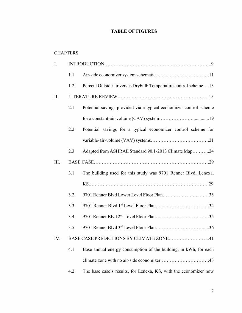
I. INTRODUCTION…………………………………………………………..9

II. LITERATURE REVIEW………………………………………………….15

III. BASE CASE…………………………….…………………………………29

Building Construction…………………………………………………….. 30

HVAC System……………………………………………………………. 30

HVAC Load and Energy Analysis Software Utilized…………………….. 37

Software Inputs…………………………………………………………….38

IV. BASE CASE PREDICTIONS BY CLIMATE ZONE……………………..41

Base Case’s Annual Energy Consumption Predictions…………………….42

V. BALANCE POINT TEMPERATURE…………………………………….53

VI. ECONOMIZER SET POINT ANALYSIS………………………………...78

VII. CONCLUSIONS AND RECOMMENDATIONS………………………...99

VIII. APPENDIX………………………………………………………………102

IX. REFERENCES...…………………………………………………………106

X. BIBLIOGRAPHY…..……………………………………………………107

2

TABLE OF FIGURES

CHAPTERS

I. INTRODUCTION…………………………………………………………..9

1.1 Air-side economizer system schematic…………………………….11

1.2 Percent Outside air versus Drybulb Temperature control scheme….13


2.1 Potential savings provided via a typical economizer control scheme

for a constant-air-volume (CAV) system…………………..............19

2.2 Potential savings for a typical economizer control scheme for

variable-air-volume (VAV) systems……………………………….21

2.3 Adapted from ASHRAE Standard 90.1-2013 Climate Map………..24

III. BASE CASE……………………………………………………………….29

3.1 The building used for this study was 9701 Renner Blvd, Lenexa,

KS.………………...……………………………………………….29

3.2 9701 Renner Blvd Lower Level Floor Plan…………………...……33

3.3 9701 Renner Blvd 1st Level Floor Plan…………………………….34

3.4 9701 Renner Blvd 2nd Level Floor Plan…………………………….35

3.5 9701 Renner Blvd 3rd Level Floor Plan………………………….....36


4.1 Base annual energy consumption of the building, in kWh, for each

climate zone with no air-side economizer………………………….43

4.2 The base case’s results, for Lenexa, KS, with the economizer now

3

active, but with the low-limit varied………………………………..44

4.3 Zone 1A – Miami, FL……………………………………………...44

4.4 Zone 2A – Houston, TX……………………………………………45

4.5 Zone 2B – Phoenix, AZ………………………………………….....45

4.6 Zone 3A – Atlanta, GA…………………………………………….46

4.7 Zone 3B – Los Angeles, CA………………………………………..46

4.8 Zone 3C – San Francisco, CA………………………………...........47

4.9 Zone 4A – Baltimore, MD………………………………………....47

4.10 Zone 4B – Albuquerque, NM……………………………………....48

4.11 Zone 4C – Seattle, WA………………………………………….....48

4.12 Zone 5A – Chicago, IL……………………………………………..49

4.13 Zone 5B – Boulder, CO…………………………………………….49

4.14 Zone 5C – Vancouver, BC………………………………………....50

4.15 Zone 6A – Minneapolis, MN……………………………………....50

4.16 Zone 6B – Helena, MT……………………………………………..51

4.17 Zone 7 – Duluth, MN……………………………………………....51

4.18 Zone 8 – Fairbanks, AK…………………………………………....52

V. BALANCE POINT TEMPERATURE…………………………………….53

5.1 Building Balance Point Temperature Worksheet…………………..59

5.2 Collecting floor area square footage from a Trane Trace System

Checksum report…………………………………….......................61

5.3 Building balance point temperature worksheet with the example’s U-

values and floor area entered……………………………………….62

4

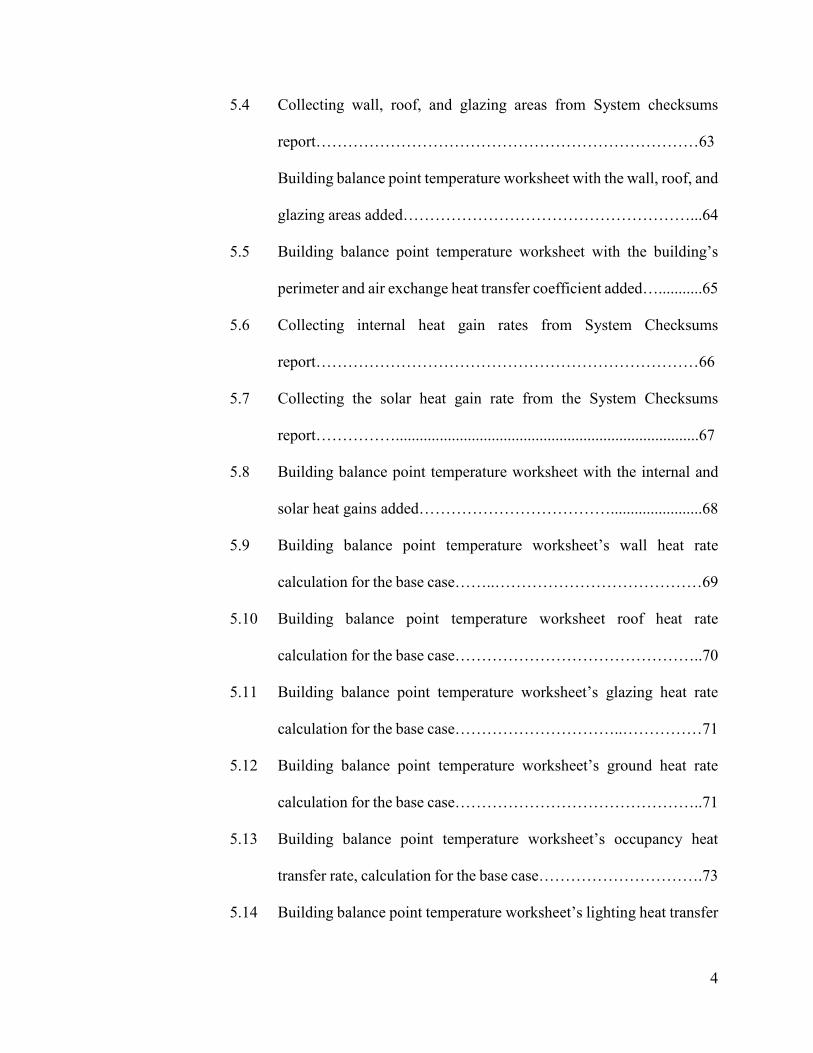
5.4 Collecting wall, roof, and glazing areas from System checksums

report………………………………………………………………63

Building balance point temperature worksheet with the wall, roof, and

glazing areas added………………………………………………...64

5.5 Building balance point temperature worksheet with the building’s

perimeter and air exchange heat transfer coefficient added…...........65

5.6 Collecting internal heat gain rates from System Checksums

report………………………………………………………………66

5.7 Collecting the solar heat gain rate from the System Checksums

report……………............................................................................67

5.8 Building balance point temperature worksheet with the internal and

solar heat gains added……………………………….......................68

5.9 Building balance point temperature worksheet’s wall heat rate

calculation for the base case……..…………………………………69

5.10 Building balance point temperature worksheet roof heat rate

calculation for the base case………………………………………..70

5.11 Building balance point temperature worksheet’s glazing heat rate

calculation for the base case…………………………..……………71

5.12 Building balance point temperature worksheet’s ground heat rate

calculation for the base case………………………………………..71

5.13 Building balance point temperature worksheet’s occupancy heat

transfer rate, calculation for the base case………………………….73

5.14 Building balance point temperature worksheet’s lighting heat transfer

5

rate calculation for the base case.......................................................73

5.15 Building balance point temperature worksheet’s equipment heat

transfer rate calculation for the base case…………………………..74

5.16 Building balance point temperature worksheet’s solar heat transfer

rate calculation for the base case…………………………………...75

5.17 Building balance point temperature worksheet’s final calculation for

the base case………………………..................................................76


6.1 Results for the base case in Lenexa, KS with points and ranges of

interest……………………………………......................................81

6.2 Results for Zone 1A in Miami, FL with points and ranges of interest

……………………………………………......................................82

6.3 Results for Zone 2A in Houston, TX with points and ranges of interest

……………………………………………………………………..83

6.4 Results for Zone 2B in Phoenix, AZ with points and ranges of interest

………………………….……………….........................................84

6.5 Results for Zone 3A in Atlanta, GA with points and ranges of interest

……………………………..……………………………………....85

6.6 Results for Zone 3B in Los Angeles, CA with points and ranges of

interest ……………………..……………………………………...86

6.7 Results for Zone 3C in San Francisco, CA with points and ranges of

interest …………………...………………......................................87

6.8 Results for Zone 4A in Baltimore, MD with points and ranges of

6

interest …………….………………………………………………88

6.9 Results for Zone 4B in Albuquerque, NM with points and ranges of

interest …………………………………………………………….89

6.10 Results for Zone 4C in Seattle, WA with points and ranges of interest

……………………….….………………………………………....90

6.11 Results for Zone 5A in Chicago, IL with points and ranges of interest

……………………..………………………………………………91

6.12 Results for Zone 5B in Boulder, CO with points and ranges of interest

………………….………………………………………………….92

6.13 Results for Zone 5C in Vancouver, BC with points and ranges of

interest ………………….…………………………………………93

6.14 Results for Zone 6A in Minneapolis, MN with points and ranges of

interest …………….………………………………………………94

6.15 Results for Zone 6B in Helena, MT with points and ranges of interest

…………………..…………………………………………………95

6.16 Results for Zone 7 in Duluth, MN with points and ranges of interest

…………………….……………………………………………….96

6.17 Results for Zone 8 in Fairbanks, AK with points and ranges of interest

……………….…………………………………………………….97


7

TABLE OF TABLES

CHAPTERS

I. INTRODUCTION…………………………………………………………..9


2.1 High-limit control for integrated economizers……………..………16

2.2 Adapted from ASHRAE Standard 90.1-2013 Table 6.5.1-1….........24

2.3 Adapted from ASHRAE Standard 90.1-2013 Table 6.5.1-2 ………25

2.4 Adapted from ASHRAE Standard 90.1-2013 Table 6.5.1-3……….25

III. BASE CASE……………………………………………………………….29

3.1 Electricity Usage from 2006 to 2012…………………………….....31

3.2 Lighting, office, and miscellaneous loads………………………….40


4.1 Location selected within each North American climate zone............42

V. BALANCE POINT TEMPERATURE……….……………………………53

Building Balance Point Temperature Worksheet Units……..………..........58


6.1 Calculated balance point temperature for each climate zone for the

base case building…….....................................................................79

6.2 Base case energy consumption or savings (kWh).............................81

6.3 Zone 1A energy consumption or savings (kWh)…………………...82

6.4 Zone 2A energy consumption or savings (kWh)…….......................83

6.5 Zone 2B energy consumption or savings (kWh)…….......................84

8


6.7 Zone 3B energy consumption or savings (kWh)…………………...86

6.8 Zone 3C energy consumption or savings (kWh)…………………...87



6.11 Zone 4C energy consumption or savings (kWh)…………………..90


6.13 Zone 5B energy consumption or savings (kWh)…………………..92

6.14 Zone 5C energy consumption or savings (kWh)…………………...93

6.15 Zone 6A energy consumption or savings (kWh)…………………..94


6.17 Zone 7 energy consumption or savings (kWh)……………………..96

6.18 Zone 8 energy consumption or savings (kWh)……………………..97


9

CHAPTER I

INTRODUCTION

The Industrial Revolution led many scientists and inventors to create new and to

improve existing heating, ventilation, and air conditioning (HVAC) systems. In the present

decade, the struggle is mainly to create more energy efficient HVAC equipment. Currently

standards and codes require increasingly energy efficient HVAC systems, and that translates

directly into energy savings for their users and reduced carbon emissions from most of the

power plants that provide the needed electricity.

One HVAC device that has the potential for increasing energy efficiency in certain

buildings and climates is the airside economizer. This is a control scheme intended to reduce

cooling-mode energy consumption. When the outside air (OA) is cool, more air is introduced

to replace or supplement the cooling and possibly the dehumidification that is provided by

the cooling coil. For small commercial, institutional, and industrial (CII) buildings with

packaged HVAC air handlers such as rooftop units (RTUs), adding simple dry-bulb

temperature economizers with commonly-used fixed control setpoints will not produce

optimal performance because airborne moisture is not considered. However, enthalpy

controllers with multiple sensors have the ability to calculate the current heat balance,

including the effects of moisture. They help to provide superior thermal performance but at

a significantly increased initial cost; they typically need more maintenance as well. Dry-bulb

control is thus more common; however, not monitoring the moisture introduced via the OA

leads to increased energy consumption and periods of decreased thermal comfort as

compared to enthalpy control.

10

An air-side economizer system has outdoor air, exhaust air, and recirculated air

dampers to regulate these air flow rates. The dampers, and their attached ductwork, are sized

to allow up to 100% of the required cooling supply airflow to be outside air. The recirculated

air is the difference between the supply airflow and the exhaust airflow. When the OA is

warm and humid the recirculated air damper is open to its maximum position, the exhaust

air and OA dampers are in their minimum-for-ventilation-needs position. When the OA is

cool and dry, the air-side economizer modulates the outdoor, exhaust, and recirculated air

dampers, providing all necessary cooling via increased outside air flow, or to reduce the

needed mechanically-provided cooling when the OA is of moderate temperature. Figure 1.1

is a schematic of an air-side economizer where:

11

Figure 1.1 Air-side economizer system schematic

1. Return air (RA)

2. Recirculated air (CA) and its damper

3. Exhaust air (EA), its damper, and the EA fan

4. Outdoor air (OA) and its damper

5. Mixed air (MA) and air filter

6. Supply air (SA), and the SA fan

Figure 1.2 shows a drybulb temperature economizer control scheme, with the

percentage of OA admitted varying with the temperature of the OA. Below the low-limit,

the building is in space heating mode and only the minimum flow rate of outside air needed

for ventilation is admitted. The low-limit OA temperature is at the point when the building

should switch from heating to cooling mode. With an air-side economizer, as the cooling

12

load increases the interlinked OA, CA, and EA dampers modulate to maintain the

temperature of the indoor spaces; without the economizer the minimum OA would continue

to be admitted but the mechanical cooling system would be activated. But with the drybulb

airside economizer, above the low-limit, as shown in Figure 1.2, the percentage of OA

increases linearly with the temperature of the OA. The system is in “free”-cooling mode,

until it reaches the middle-limit where there is 100% OA and the temperature of the OA is

typically 55°F (12.8°C), the common design supply air temperature during cooling mode.

As the outdoor temperature increases above the middle-limit, the OA remains constant at

100% but the mechanical cooling is activated to keep the supply air at 55°F (12.8°C). Once

the temperature of the OA reaches the high-limit, the percentage of OA is reduced to the

minimum-ventilation required once again to minimize mechanical cooling energy

consumption. This minimum percent OA is typically 10 to 20% for code-compliant office

buildings in the United States.

13

Figure 1.2 Percent Outside air versus Drybulb Temperature control scheme

For these simple, widely-used dry-bulb controllers, the three OA temperature

setpoints of concern are thus 1) the low-limit, where need for indoor cooling begins, 2) full

“free-cooling” middle-limit where the mixed air temperature matches the design cooling-

mode supply air temperature, and 3) the high-limit where the percent OA is decreased to the

minimum because the OA is too warm or humid. Other researchers have studied the high-

limit in detail, e.g., Taylor and Cheng 2010, and have produced practical advice for selecting

it. The middle-limit is the cooling mode design supply air temperature as specified by the

design engineer and is often 55°F (12.8°C) for conventional HVAC systems in North

14

America.

Researchers have not previously focused on the effect of low-limit setpoints. The

low-limit setpoint is problematic, as it is normally assumed equal to the building’s balance

point temperature, which is an unknown. However, due to lack of knowledge as to what that

low-limit should be set to, the installer will often guess the balance point temperature. As a

result, energy consumption will be higher than optimal either by over- or under-cooling the

building unless the installer makes an excellent estimate of the optimal setpoint.

The purpose of this research study was to examine the effect of dry-bulb low-limits

on the annual cooling energy consumption of an office building in various climates. While

the high-limit is discussed, it was not the focus of this study.

An existing occupied building was selected as the base case for the study for realism

and because actual energy usage records were obtainable. In a later chapter the base case

will be discussed in detail. The building’s annual energy performance, without utilizing an

airside economizer, was then simulated using an hour-by-hour computational model for

different climates of the United States. By doing so the balance point temperature could be

observed. Then the simulations were performed again but with the airside economizer

activated and the low-limits set to these balance point temperatures in each of the different

climate zones. In addition, the low-limit was varied through a range of other temperatures

thus allowing for the comparison of energy savings to observe the optimal values. However,

before the simulations were performed, a literature review was conducted, and its results

appear in Chapter II of this thesis.

15

CHAPTER II

LITERATURE REVIEW

New mid- to large-sized buildings’ HVAC systems often employ air- or water-side

economizers. While economizers have been around for decades, it is within the last ten years

or so that the use of an economizer was strongly suggested or even outright required by

building energy conservation codes such as ANSI/ASHRAE Standard 90.1 (ASHRAE 90.1-

2013). The benefit of the airside economizer is that free- or reduced-cost cooling can be

accomplished similarly to natural ventilation schemes but without the problems of natural

ventilation such as less-than-optimal user operation of windows (Emmerich et al. 2003).

Different types of air-side economizer control strategies exist. Types of airside

economizers include fixed drybulb, differential dry bulb, fixed enthalpy, electronic enthalpy,

differential enthalpy, and dewpoint-and-drybulb. The fixed drybulb is simple: when the

outside air (OA) increases to a fixed temperature of about 68°F (20°C) to 72°F (22.2°C), the

economizer is disabled so that dampers return to the minimum position needed for admitting

ventilation air. With differential drybulb, the economizer becomes disabled when the OA is

warmer than the return air. Similar to fixed drybulb, the fixed enthalpy type is disabled when

the OA reaches a fixed enthalpy. When the OA reaches a predefined high-limit drybulb and

dewpoint, the electronic enthalpy type disables the economizer. In the case of differential

enthalpy, an economizer will be disabled when the return air enthalpy is less than the OA

enthalpy. Once achieving the desired fixed dewpoint or drybulb, the dewpoint-and-drybulb

type reduces the percent OA. To achieve the goal of uniform compliance with ASHRAE

Standard 90.1, one of these economizers is often required. Before this code mandate, the air-

16

side economizer control scheme selected, if any, was dependent on the desired initial cost of

the system and the predicted operating costs (Trane 2006).

According to Taylor et al. (2010), each of the different types of control systems and

their schemes introduce errors. Their study showed this causes an increased use of energy

when compared to theoretically perfect control logic and performance. Using the different

climate zones provided in ASHRAE 90.1, they developed a table of proposed high limits.

Taylor et al. (2010) gives these high limits based upon device type, climate zone, and high-

limit logic. Also included in this table are the device types that would not be recommended

for each climate zone. Table 2.1 displays these values.

Table 2.1 High-limit control for integrated economizers [Taylor et al. 2010]

Device TypeAcceptable in Climate

Zone at Listed Setpoint

Not Recommended In

Climate Zone

Equation Description

3C, 6B, 8 TOA > 75°F Outdoor air tempurature exceeds 75°F

1B, 2B, 3B, 4B, 4C, 5B TOA > 73°F Outdoor air tempurature exceeds 73°F

5C, 6A, 7 TOA > 71°F Outdoor air tempurature exceeds 71°F

1A, 2A, 3A, 4A, 5A TOA > 69°F Outdoor air tempurature exceeds 69°F

Differential Dry Bulb1B, 2B, 3B, 3C, 4B, 4C, 5B,

5C, 6B, 7, 8TOA > TRA

Outdoor air tempurature exceeds

return air tempurature1A, 2A, 3A, 4A, 5A, 6A

Fixed Enthalpy 4A, 5A, 6A, 7, 8 hOA > 28 Btu/lb*Outdoor air enthalpy exceeds 28 Btu/lb

of dry air*All

Fixed Enthalpy + Fixed

Dry BulbAll

hOA > 28 Btu/lb* or

TOA > 75°F

Outdoor air enthalpy exceeds 28 Btu/lb

of dry air* or outdoor air dry bulb

exceeds 75°F

All

Electronic Enthalpy All (TOA ,RHOA ) > AOutdoor air tempurature/RH exceeds

the "A" setpoint curve.†All

Differential Enthalpy None hOA > hRA

Outdoor air enthalpy exceeds return air

enthalpy. All

Differential Enthalpy

+ Fixed (or

Differential) Dry Bulb

NonehOA > HRA or TOA > 75°F

(or TRA)

Outdoor air enthalpy exceeds return air

enthalpy or outdoor air dry bulb

exceeds 75°F (or return air

tempurature)

All

Dew Point + Dry-Bulb

TempuraturesNone

DPOA > 55°F or TOA >

75°F

Outdoor dew point exceeds 55°F (65

gr/lb) or outside air dry bulb exceeds

75°F

All

High Limit Logic (Economizer Off When):

Fixed Dry Bulb

* At altitudes substantially different than sea level, the fixed enthalpy limit shall be set to the enthalpy value at 75°F and 50% relative

humidity. As an example, at approximately 6,000 ft elevation the fixed enthalpy limit is approximately 30.7 Btu/lb

† Setpoint "A" corresponds to a curve on the psychrometric chart that goes through a point at approximately 73°F and 50% rela<ve

humidity and is nearly parallel to dry-bulb lines at low humidity levels and nearly parallel to enthalpy lines at hugh humidity levels.

17

Another concern associated with air-side economizer control is that building

pressurization can affect adversely its performance. If the HVAC system brings in OA

without providing a way for the extra air to escape, the building will develop excess indoor

air pressure, have difficulty in bringing in more OA, create moisture concerns in the building

enclosure, and have troubles with exterior doors’ operation. Besides increasing the ducted

exhaust airflow rate, ways exist to reduce this excess building pressure, one of which is the

use of local barometric relief dampers that are also known as gravity dampers. When using

an air-side economizer device some method of building pressure control must be

implemented (Trane 2006).

A constant-air-volume (CAV) system control scheme for an air-side economizer is

slightly different than the control scheme for a variable-air-volume (VAV) system. In cold

weather, the heating load of the admitted OA decreases as the OA temperature rises toward

the low-limit. The overall heating load is the heat rate added to a space to maintain the

building temperature; the cold OA that’s admitted is a portion of this heating load. To

minimize energy consumption, the minimum OA airflow needed for ventilation enters the

system when in heating mode. Above the low-limit, the building’s load changes from heating

to cooling. Even if mechanical cooling isn’t provided, above the low-limit the ventilation

system can enter modulated or “free-cooling” economizer mode, where the minimum then

up to 100% OA is admitted to provide sufficient cooling until the middle-limit is reached.

With CAV, the OA and recirculated air flow rates modulate inversely to maintain the space

temperature as the building cooling load varies; the total SA flowrate remains the same. In

buildings with mechanical air-conditioning, above the middle-limit that mechanical cooling

and dehumidification is increasingly employed but 100% OA is maintained until the high-

18

limit is reached because the OA’s enthalpy is still hopefully below that of the return air. In

Figure 2.1, the dark grey area represents the mechanical cooling energy saved when the

system is in modulated economizer mode as compared to cooling with just the minimum OA

needed for ventilation. Between the low- and middle-limits, the OA damper gradually opens

from minimum to 100% as the cooling load increases. As this occurs, the recirculated air-

damper gradually closes. The system is in integrated economizer mode when 100% OA is

providing part of the cooling capacity necessary. When the building is in an unoccupied

period, small- to mid-sized mechanical cooling systems often cycle on/off as needed to

maintain the temperature within the space. In Figure 2.1, the white area represents the energy

savings when the economizer is in integrated economizer mode. After reaching the high-

limit, the integrated economizer mode will deactivate; the system will then return to

mechanical cooling-only, with the minimum required OA flow for ventilation (Trane 2006).

19

Figure 2.1 Potential savings provided via a typical economizer control scheme

for a constant-air-volume (CAV) system (Trane 2006).

In heating mode the temperature difference between the supply air (SA) and the

indoor setpoint can be very high. As a result, with VAV instead of CAV, the supply air flow

rate is likely far less than the maximum supply air flow rate typical for the design cooling-

load conditions when the design room-to-supply air temperature difference is much smaller

than for heating; in VAV systems the maximum heating SA flow rate is often only about

half that of the maximum cooling flow rate. Modulated economizer mode begins at the low-

limit when the cooling load begins to increase, but with VAV only the OA flow rate

increases, not necessarily the recirculated air, so less air may need to be moved. As with

CAV, during integrated economizer mode between the middle and high limits, the outdoor

20

damper is 100% open, and the cooling coil is active. Fans and dampers are modulated to

provide an air pressure balance. As with CAV, the system will enter mechanical cooling

with minimum required OA mode after having reached the high-limit as seen in Figure 2.2.

With VAV, the supply and return airflow rates increase to meet higher cooling loads, and

the cooling coil provides the necessary cooling and dehumidification capacity.

21

Figure 2.2 Potential savings for a typical economizer control scheme for

variable-air-volume (VAV) systems (Trane 2006).

Another concern with air-side economizers is sensor placement because the sensors’

readings will greatly affect the performance of the control scheme. The placement can affect

the operation and maintenance costs too. In addition to the sensor placement, the type of

sensor is important as well. As previously stated, a variety of controls and sensors are

available.

Properly calibrated sensors are important. ASHRAE Standard 90.1-2013 contains a

section on required sensor accuracy for air-side economizers [ASHRAE 90.1-2013,

§6.5.1.1.6]:

Outdoor air, return air, mixed air, and supply air sensors shall

22

be calibrated within the following accuracies: a. dry-bulb temperatures shall be accurate to ±2°F over the range of 40°F to 80°F; b. enthalpy and the value of a differential enthalpy sensor shall be accurate to ±3 Btu/lb over the range of 20 to 36 Btu/lb; c. relative humidity shall be accurate to ±5% over the range of 20% to 80% RH.

From this section of ASHRAE Standard 90.1-2013, it is easy to see how accurate a system

must be, because as previously noted a small difference in sensor readings can greatly affect

the accuracy and thus the efficiency of the system.

One of the requirements in ASHRAE Standard 90.1 in regards to economizers is that

the mechanical cooling systems must integrate the economizer system; “integration” means

that the economizer system becomes a part of the mechanical cooling system. According to

Standard 90.1-2013, §6.5.1.3,

Economizer systems shall be integrated with the mechanical cooling system and shall be capable of providing partial cooling even when additional mechanical cooling is required to meet the remainder of the cooling load. Controls shall not be a false load on the mechanical cooling systems by limiting or disabling the economizer or by any other means, such as hot gas bypass, except at the lowest stage of mechanical cooling.

When sizing an air-side economizer system, the system must have the appropriate design

capacity. ASHRAE Standard 90.1-2013 states, “Air economizer systems shall be capable of

modulating OA and return air dampers to provide up to 100% of the design supply air

quantity as OA for cooling.”

This requirement continues in Section 6.5.1, Economizers, of Standard 90.1-2013,

which states that “Each cooling system that has a fan shall include either an air or water

economizer meeting the requirements of sections 6.5.1.1 through 6.5.1.6.” The exceptions

are [ASHRAE 90.1-2013, §6.5.1]:

23

1. Individual fan-cooling units with a supply capacity less than the minimum listed in Table 6.5.1-1 for comfort cooling applications and Table 6.5.1-2 for computer room applications.

2. Systems that include nonparticulate air treatment as required by Section 6.2.1 in Standard 62.1.

3. In hospitals and ambulatory surgery centers, where more than 75% of the air designed to be supplied by the system is to spaces that are required to be humidified above 35°F dew-point temperature to comply with applicable codes or accreditation standards; in all other buildings, where more than 25% of the air designed to be humidified above 35°F dew-point temperature to satisfy process needs. This exception does not apply to computer rooms.

4. Systems that include a condenser heat recovery system with a minimum capacity as defined in Section 6.5.6.2.2.

5. Systems that serve residential spaces where the system capacity is less than five times the requirement listed in Table 6.5.1-1.

6. Systems that serve spaces whose sensible cooling load at design conditions, excluding transmission and infiltration loads, is less than or equal to transmission and infiltration losses at an outdoor temperature of 60°F.

7. Systems expected to operate less than 20 hours per week.

8. Where the use of outdoor air for cooling will affect supermarket open refrigerated casework systems.

9. For comfort cooling where the cooling efficiency meets or exceeds the efficiency improvement requirements in Table 6.5.1-3.

10. Systems primarily serving computer rooms where a. the total design cooling load of all computer

rooms in the building is less than 3,000,000 Btu/h and the building in which they are located is not served by a centralized chilled water plant;

b. the room total design cooling load is less than 600,000 Btu/h and the building in which they are located is served by a centralized chilled water plant;

c. the local water authority does not allow cooling towers; or

d. less than 600,000 Btu/h of computer-room

24

cooling equipment capacity is being added to an existing building

11. Dedicated systems for computer rooms where a minimum of 75% of the design load serves

a. those spaces classified as an essential facility, b. those spaces having a design of Tier IV as

defined by ANSI/TIA-942, c. those spaces classified under NFPA 70 Article

708 – Critical Operations Power Systems (COPS), or

d. those spaces where core clearing and settlement services are performed such that their failure to settle pending financial transactions could present systemic risk as described in “The Interagency Paper on Sound Practices to Strengthen the Resilience of the U.S. Financial System, April 7, 2003”

The tables mentioned in this list of exceptions are repeated in this thesis as Tables

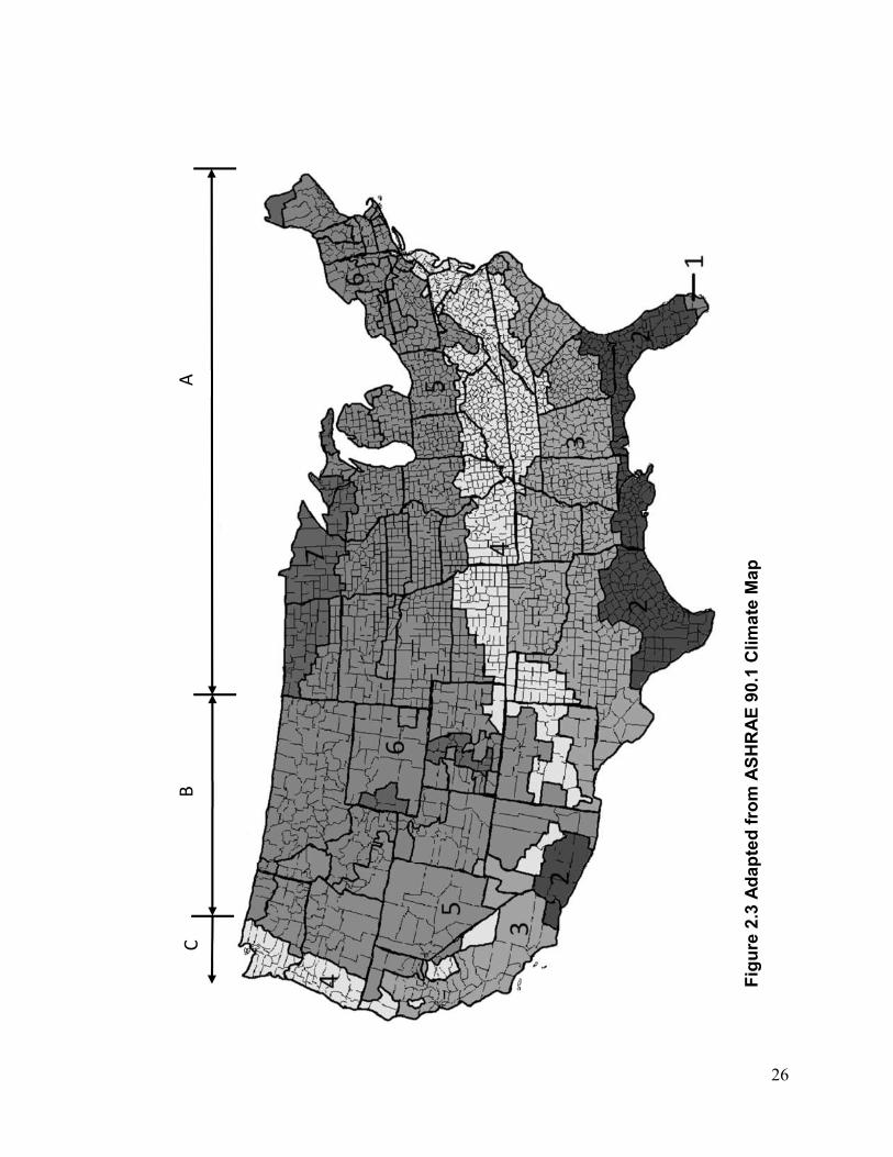
2.2 through 2.4. Figure 2.3, from ASHRAE 90.1 is an adapted climate zone map.

Table 2.2 Adapted from ASHRAE Standard 90.1-2013 Table 6.5.1-1

Climate ZonesCooling Capacity for which

an Economizer is Required

1a, 1b No economizer requirement

1a, 2b, 3a, 4a, 5a, 6a, 3b, 3c,

4b, 4c, 5b, 5c, 6b, 7, 8≥54,000 Btu/h

Minimum Fan-Cooling Unit Size for which an Economizer

is Required for Comfort Cooling

25



Climate ZonesCooling Capacity for which

an Economizer is Required

1a, 1b No economizer requirement

1a, 2b, 3a, 4a, 5a, 6a, 3b, 3c,

4b, 4c, 5b, 5c, 6b, 7, 8≥54,000 Btu/h

Minimum Fan-Cooling Unit Size for which an Economizer

is Required for Comfort Cooling

Climate Zone Efficiency Improvement ͣ

2a 17%

2b 21%

3a 27%

3b 32%

3c 65%

4a 42%

4b 49%

4c 64%

5a 49%

5b 59%

5c 74%

6a 56%

6b 65%

7 72%

8 77%

Eliminate Required Economizer for Comfort Cooling by

Increasing Cooling Efficiency

a. If a unit is rated with an IPLV, IEER, or SEER then to eliminate the required

air or water economizer, the minimum cooling efficiency of the HVAC unit

must be increased by the percentage shown. If the HVAC unit is only rated

with a full-load metric like EER cooling then these must be increased by the

percentage shown

26

Fig

ure

2.3

Ad

ap

ted

fro

m A

SH

RA

E 9

0.1

Clim

ate

Ma

p

C

B

A

27

Minimum ventilation air requirements for commercial and institutional buildings are

defined in ASHRAE Standard 62.1. That minimum is “The outdoor air flow required in the

breathing zone of the occupiable space or spaces in a ventilation zone, i.e., breathing zone

outdoor air flow (Vbs), shall be no less than the value determined in accordance with Equation

6.2.2.1” (ASHRAE 62.1-2013). Equation 6.2.2.1 of the standard is shown as Equation 2.1

of this thesis.

Vbz = Rp x Pz + Ra x Az (2.1)

where

Az represents the floor area of the zone, ft2 (m2)

Pz is the population of the zone, number of people

Rp is the outside airflow rate per person, and

Ra is the outside airflow rate per unit floor area.

Values for both Rp and Ra are given in Table 6.2.2.1 of Standard 62.1-2013 (ASHRAE 2013).

The design engineer for such a system will need to examine the various operational

conditions over the entire year. For a data processing center with no economizer, for

example, the cooling system might need to run all 8,760 hours per year to remove the heat

released by the many continuously-operating computers and networking devices within. Due

to this, the potential for savings via the use of an air-side economizer is great, depending on

the climate and other factors.

As such, one of the most common applications of economizers, aside from office

buildings, is in data centers. Data centers are a major energy consumer. The concerns with

28

airside economizers’ use in data centers pertain to outdoor particulates and other

contaminants making their way into the building, as well as the ability to control the

humidity within the spaces served. Many of the concerns relating to OA in data centers are

being addressed in ASHRAE’s Technical Committee (TC) 9.9. While there is apprehension,

more engineers and designers are using airside economizers in data centers, and data centers

are often intentionally being built in cold climates rather than warm.

Most recently in Santa Clara, California, in Building 4 of the Marvell Semiconductor

U.S. headquarters, an airside economizer was installed on an existing data center; Santa

Clara has a mild, but not cold climate. These project retrofitted airside economizers on to

the already installed computer room air handlers (CRAHs). With an uninterruptible power

supply added too as part of the project, the cost was approximately US$662,000. Once the

project was completed and the economizers were functioning properly, the City of Santa

Clara’s electrical utility awarded a rebate of US$171,000. Before the completion of the

project, the electrical energy consumption for the 12 months prior was approximately

1,361,450 kWh per month. After completion of the project, the building was, on average,

consuming 1,091,280 kWh per month, resulting in a 270,170 kWh reduction per month. This

was a 20% reduction in the overall building electrical energy consumption and 30% in the

data center. With US$27,000 per month savings in energy costs, the simple payback was

only 18 months [Alipour 2013].

Despite the large potential energy savings through the use of airside economizers,

when properly specified, installed, and operated, many such control schemes never achieve

their design intent. Identifying and then using optimal setpoints is essential in achieving the

desired energy savings, and best thermal comfort.

29

CHAPTER III

BASE CASE

The commercial building used in this study is in Lenexa, Kansas at 9701 Renner Boulevard.

In 2006, the building was completed and occupancy of it began. The gross building area is

129,321 square feet, and the net usable area is 108,096 square feet, with four floors to the

building. Trees and shaded areas surrounding the building are sparse and offer little to no

shading on the building’s exterior as is shown in Figure 3.1

Figure 3.1 The building used for this study was 9701 Renner Blvd, Lenexa,

KS.

30

Building Construction

The building has a large number of windows. The glazings in the building are double-

pane 0.2362 inch (6 mm) tinted glass. The U-value of the windows are 0.505 Btu/h·ft2·°F

(2.87 W/m2·K). The exterior walls have precast concrete on their outside and standard

gypsum wallboard on the inside. Due to not having the exact composition of the construction

materials on the inside of the walls, the overall heat transfer coefficient (U-value) of the wall

assembly was assumed to be typical for this type of building at approximately 0.0526

Btu/h·ft2·°F (0.297 W/m2·K). Similarly, the U-value of the roof assembly was assumed to

be approximately 0.0333 Btu/h·ft2·°F (0.189 W/m2·K). The floor slab of the building is

assumed to be 8 inch thick (0.2032 m) heavyweight concrete.

HVAC System

For typical large United States commercial office buildings the most common HVAC

system used is variable-air-volume (VAV) with reheat; the base case building uses such and

is also all-electric as are many such buildings; no natural gas is utilized. Each floor of the

building was split by its HVAC designer into multiple thermal zones. As such, in this study,

the base case included an all-air HVAC system with VAV terminal units with electric

resistance reheat serving the many thermal zones. To establish the base energy consumption

per year each of the first group of simulations had the same system with only the

geographical location of the building changed. In the second set of simulations, the airside

economizer was activated. Initially these airside economizer cases kept the low-, middle-,

and high-limit set points of the economizer as the defaults of the simulation program; later

the low-limit was varied.

The actual building’s monthly electricity use was recorded by a facilities manager

31

from the January 2006 to through November 2012. In 2012, the overall annual energy

consumption was lower than the average for the six years prior. From December 2012 to

2013 the building was not fully occupied, so those months’ data were not utilized for this

study. Table 3.1 shows the monthly electrical energy use of the building.

Table 3.1 Electricity Usage from 2006 to 2012 (Courtesy of Kiewit)

Electricity Usage

kWh

2006 2007 2008 2009 2010 2011 2012

JAN 304,800 336,800 322,800 328,000 303,200 331,200 275,200

FEB 346,400 366,000 386,800 296,000 295,600 304,400 290,400

MAR 277,200 253,200 328,000 249,600 252,400 252,800 211,200

APR 269,600 280,000 288,800 266,400 238,800 250,800 217,200

MAY 272,000 267,600 276,400 239,600 226,400 232,000 214,200

JUN 270,800 283,600 268,800 248,800 233,600 236,800 234,000

JUL 322,000 294,000 276,800 251,600 261,200 285,600 216,400

AUG 282,400 290,800 283,200 217,200 246,000 233,600 187,200

SEP 270,400 286,800 292,000 213,200 224,000 222,800 197,600

OCT 282,000 256,800 266,000 222,400 220,800 230,000 200,000

NOV 318,000 334,400 324,000 263,200 308,400 275,200 232,400

DEC 336,800 365,600 353,200 352,000 364,000 315,600 -

Total 3,552,400 3,615,600 3,666,800 3,148,000 3,174,400 3,170,800 2,475,800

Average 296,033 301,300 305,567 262,333 264,533 264,233 206,317

32

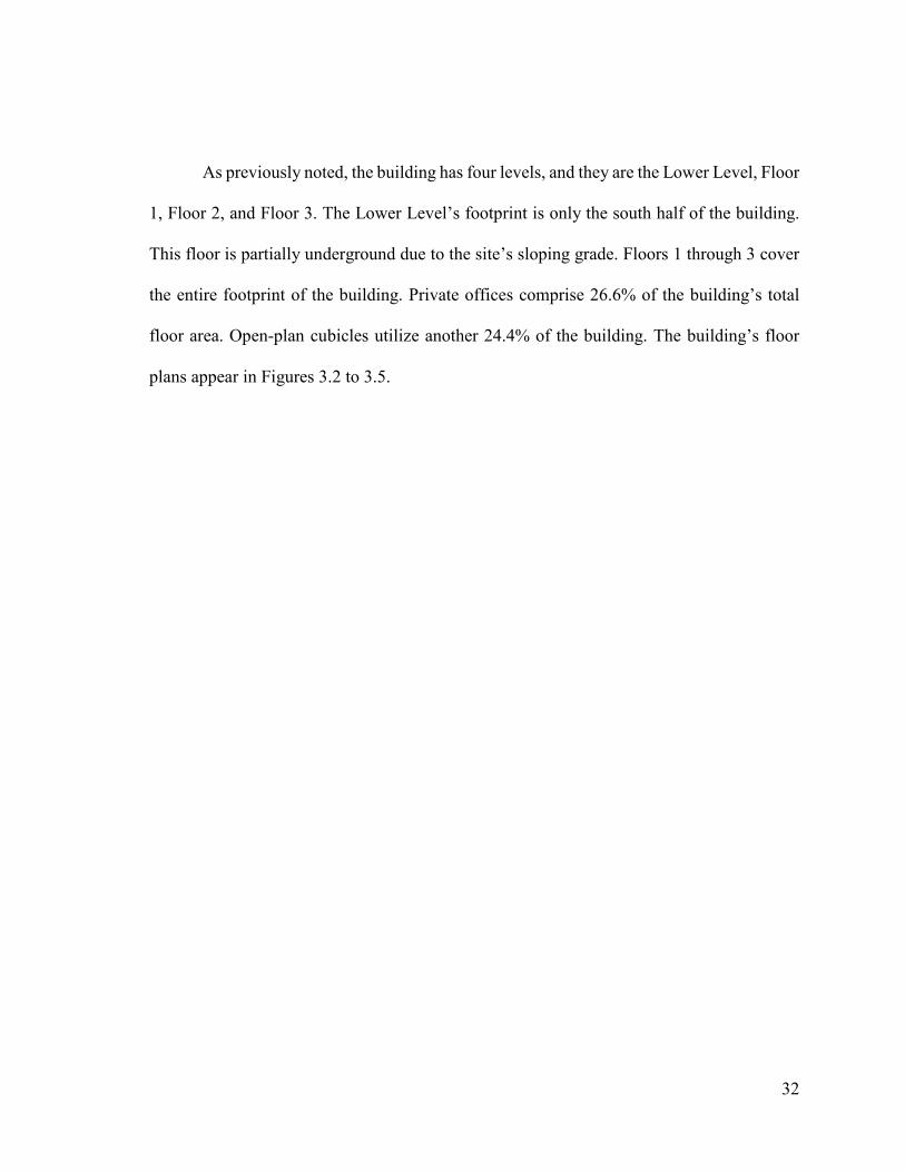
As previously noted, the building has four levels, and they are the Lower Level, Floor

1, Floor 2, and Floor 3. The Lower Level’s footprint is only the south half of the building.

This floor is partially underground due to the site’s sloping grade. Floors 1 through 3 cover

the entire footprint of the building. Private offices comprise 26.6% of the building’s total

floor area. Open-plan cubicles utilize another 24.4% of the building. The building’s floor

plans appear in Figures 3.2 to 3.5.

33

Fig

ure

3.2

97

01 R

en

ne

r B

lvd

Lo

we

r L

eve

l F

loo

r P

lan

34

Fig

ure

3.3

97

01 R

en

ne

r B

lvd

1s

t L

eve

l F

loo

r P

lan

35

Fig

ure

3.4

97

01 R

en

ne

r B

lvd

2n

d L

eve

l F

loo

r P

lan

36

Fig

ure

3.5

: 9

70

1 R

en

ne

r B

lvd

3rd

Le

ve

l F

loo

r P

lan

37

HVAC Load and Energy Analysis Software Utilized

Two separate modeling programs were used to perform the needed thermal analyses

of the building. Trane’sTraceTM700 was used to perform the initial calculations (Trane

2013). The then-latest version, 6.3, was used. Complete with subroutines in load design,

system simulation, equipment simulation, energy consumption and economic analyses,

TraceTM700 was deemed, at least at first, a logical program for modeling the building and

the proposed HVAC system modifications.

TraceTM700 and all other building energy simulation programs require much input

data. Building descriptions that include location, zones, materials, and weather data are

needed by the load and energy calculations subroutines. Each of the HVAC systems’ input

data sets are comprised of system type, temperature and humidity setpoints, economizer

type, and dedicated OA scheme, for example. Peak and hourly loads are determined by the

load-design subroutine. Airflow and supply air temperatures by zone are extracted from the

load-design subroutine’s results and then used by the system simulation subroutine. Both the

load subroutine and the system simulation subroutine use data from a weather library. From

the system simulation subroutine, the hour-by-hour equipment loads are determined and then

utilized further in the equipment simulation subroutine. Transient equipment’ performance

descriptions such as pump and fan curves are included in the equipment simulation

subroutine via a performance library. After determining each piece of equipment’s energy

consumption, and then summing them for each primary energy source, the economic

analysis is performed by the program. However, the economic portion of the software was

not needed for this research project, only the predicted annual energy use for each case.

The second modeling software used was eQUEST; it is a user-friendly shell for DOE-

38

2 (eQuest 1999). This software was used strictly for energy modeling purposes. Version 3.65

was the most-current version of eQUEST and was utilized for this study. eQUEST is short

for “The Quick Energy Simulation Tool.” The shell program uses text-entry windows in

which the users are led through steps to define the building. Based on the initial choices

made within the software’s early input windows, there would be either more or fewer steps

taken. Through further steps, eQUEST allows the user to run simulations and then the results

are provided in user-friendly formats such as graphs and tables instead of the raw data files

of DOE-2 (eQuest 1999).

Software Inputs

Discrepancies can occur when using multiple software programs. It is important

when using different types of software that the input data match, which can be very difficult

sometimes. With TraceTM700 and eQUEST, the data entry style into the programs is

different, and the programs’ default assumptions are not necessarily the same. The biggest

instance was the dimensions. For example, in TraceTM700, each space within the building is

input separately. In eQUEST the buildings outer perimeter is entered and then the internal

spaces are all described by percentages.

The overall exterior wall area, including windows for the building is approximately

30,900 square feet. Of that area, the wall area that is glass is 60%. The solar load through all

of this glass is fairly high and does not differ much in the predicted annual peak loads for

the various sites used in the United States due to a small range of latitudes.

Similarly to glass, infiltration is an envelope load. In both TraceTM700 as well as

eQUEST, the chosen value for infiltration was 0.3 air changes per hour (ACH). This value

for infiltration applies to the perimeter of the building and is a design-estimate for a

39

commercial building with neutral pressurization.

Similarly, ventilation must be taken into account. Ventilation, as defined by

ASHRAE Standard 62.1-2013, is “the process of supplying air to or removing air from a

space for the purpose of controlling air contaminant level, humidity, or temperature within

the space” (ASHRAE 62.1-2013). The ventilation air flow rate is determined using many

factors such as number of occupants, occupancy type, floor area, and ventilation system

effectiveness. The following ventilation air flow rates were found from ASHRAE Standard

62.1-2013, and the majority of spaces resulted in 15 CFM per person. But the fitness center

needed 20 CFM per person, the restrooms required 10 CFM per person, and the

mechanical/electrical/storage spaces resulted in 0.06 CFM per square foot. Due to the

ventilation rate depending on occupancy in most spaces, also needed were the estimated

occupancy for each space. For the offices, that were the majority of spaces of the building,

the occupancy was 143 square feet per person as recommended in ASHRAE Standard 62.1.

Other spaces, such as the fitness center and the mechanical/electrical/storage spaces, had

different densities. The fitness center had 17 square feet per person and the

mechanical/electrical/storage spaces had no occupants. These maximum occupancies were

also used to determine the sensible and latent heat loads of the people, which are significant

internal cooling loads of the building.

Occupancy loads are not the only internal loads; lighting and equipment loads were

also to be modeled. The Fundamentals volume of the ASHRAE Handbook (ASHRAE 2013)

has a table of lighting’s watts per square feet, as well as for various types of office equipment.

The values used appear in Table 3.2.

40

Table 3.2 Lighting, office, and miscellaneous loads (ASHRAE 2013)

Activity Space Lighting

(W/sqft)

Office

Equipment

(W/sqft)

Miscellaneous

Equipment

(W/sqft)

Cubicals 1.1 0.5 0.0

Conference Room 1.3 1.0 1.0

Office 1.1 1.0 0.0

Breakroom 1.3 0.0 1.0

Mechanical/Electrical/Storage 1.5 0.0 10.0

Lobby 1.1 0.0 0.0

Fitness Center 0.9 0.0 1.0

Restrooms 1.1 0.0 0.0

In TraceTM700, the central cooling equipment chosen were air-cooled vapor

compression unitary RTUs, with electric resistance heating coils. In eQUEST, similar to

TraceTM700, the heating source chosen was thus electric resistance. Within both of the

programs, a standard variable air volume (VAV) with electric-resistance reheat air

distribution system was chosen; the VAV minimum flow was 30% in both models. Also

similar supply and return fan data were specified within both programs. For both the supply

and return, forward-curved centrifugal fans with variable frequency drives were selected.

Through use of the software and the aforementioned inputs and values, the programs

determined results for the base case in the various climates. Examples of some spaces’ input

for TraceTM700 can be found in the Appendix.

41

CHAPTER IV

BASE CASE PREDICTIONS BY CLIMATE ZONE

Climate zones are simply averaged geographical divisions; each zone is different

based on a variety of weather factors. To improve the accuracy of results, ASHRAE Standard

90’s committee has divided each climate zone into sub-zones A, B, and C. Sub-zone A

signifies a more moist environment, B represents a drier environment, and C is representative

of a marine environment. For example, greater-San Diego’s weather ranges from mariene

along its bay to hot and dry desert just to its east. Ideally, the environment for an airside

economizer to function at its highest effectiveness is when the building needs cooling, and

the available OA is cool and its relative humidity (RH) is low. A previous study by Taylor

et.al. Cheng, examined the effects of economizer high-limits and provided good choices for

locations for this current study of the low-limit. Table 4.1 lists these various locations.

42

Table 4.1 Locations selected within each North American climate zone

Climate Zone

Location

1A Miami, FL

2A Houston, TX

2B Phoenix, AZ

3A Atlanta, GA

3B Los Angeles, CA

3C San Francisco, CA

4A Baltimore, MD

4B Albuquerque, NM

4C Seattle, WA

5A Chicago, IL

5B Boulder, CO

5C Vancouver, BC

6A Minneapolis, MN

6B Helena, MT

7 Duluth, MN

8 Fairbanks, AK

Base Case’s Annual Energy Consumption Predictions

The first step in determining the optimal low-limits was to find the base annual

energy consumption for each of the 16 climate zones when no air-side economizer was

utilized. These values gave the basis for finding the savings potential of the air side

economizer as the low-limit was varied. The results for each of the different climate zones

appear in Figure 4.1.

43

Figure 4.1 Base annual energy consumption of the building, in kWh, for each

climate zone with no air-side economizer

Due to variations in the weather, a single airside economizer setpoint for every

climate zone may or may not be optimal. To examine this the next group of simulations was

the base case but now with an airside economizer activated with a fixed dry-bulb temperature

control. However, eQUEST’s internally-calculated high-limit setpoints differ by climate

zone. Through an iterative process, the high limit was determined, set manually for each

climate zone, and then remained constant throughout the iterations. The independent

variable was then the low-limit; its value varied from the high limit temperature to an

estimated low OA temperature for the otherwise repetitive simulations. Figures 4.2 through

Figure 4.18 show the results of these building simulations where the economizer was now

active.

2700000

2800000

2900000

3000000

3100000

3200000

3300000

3400000

3500000E

ne

rgy

Co

nsu

mp

tio

n k

Wh

Base Energy Consumption

44

Figure 4.2 The base case’s results, for Lenexa, KS, with the economizer now

active, but with the low-limit varied

Figure 4.3 Zone 1A – Miami, FL

3415000

3420000

3425000

3430000

3435000

3440000

3445000

3450000

25 30 35 40 45 50 55 60 65 70

An

nu

al

En

erg

y C

on

sum

pti

on

(k

Wh

)

On-Point Temperature (F)

Zone 1A: Miami

2900000

2950000

3000000

3050000

3100000

3150000

25 35 45 55 65

An

nu

al

En

erg

y C

on

sum

pti

on

(k

Wh

)


Base case

45

Figure 4.4 Zone 2A – Houston, TX

Figure 4.5 Zone 2B – Phoenix, AZ

3180000

3200000

3220000

3240000

3260000

3280000

3300000

3320000

3340000

25 30 35 40 45 50 55 60 65 70

An

nu

al

En

erg

y C

on

sum

pti

on

(k

Wh

)


Zone 2A: Houston

3150000

3200000

3250000

3300000

3350000

3400000

25 30 35 40 45 50 55 60 65 70 75 80

An

nu

al

En

erg

y C

on

sum

pti

on

(k

Wh

)


Zone 2B: Phoenix

46

Figure 4.6 Zone 3A – Atlanta, GA

Figure 4.7 Zone 3B – Los Angeles, CA

2950000

3000000

3050000

3100000

3150000

3200000

3250000

25 30 35 40 45 50 55 60 65 70

An

nu

al

En

erg

y C

on

sum

pti

on

(k

Wh

)


Zone 3A: Atlanta

2900000

2950000

3000000

3050000

3100000

3150000

3200000

3250000

25 30 35 40 45 50 55 60 65 70 75 80

An

nu

al

En

erg

y C

on

sum

pti

on

(k

Wh

)


Zone 3B: Los Angeles

47

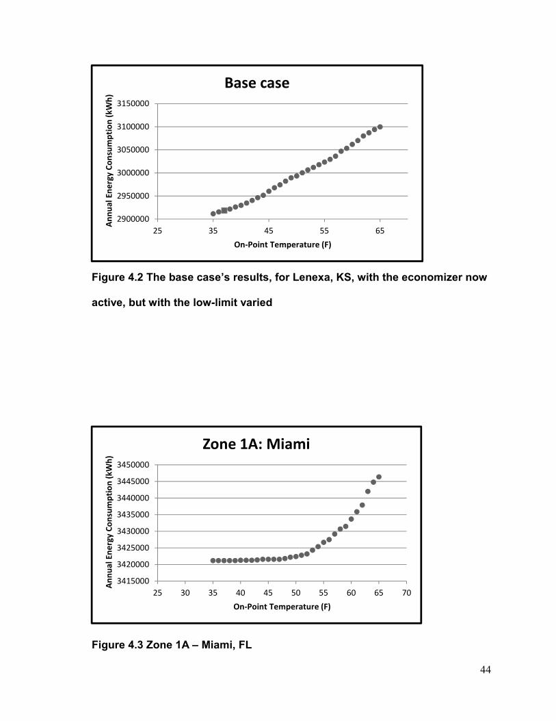
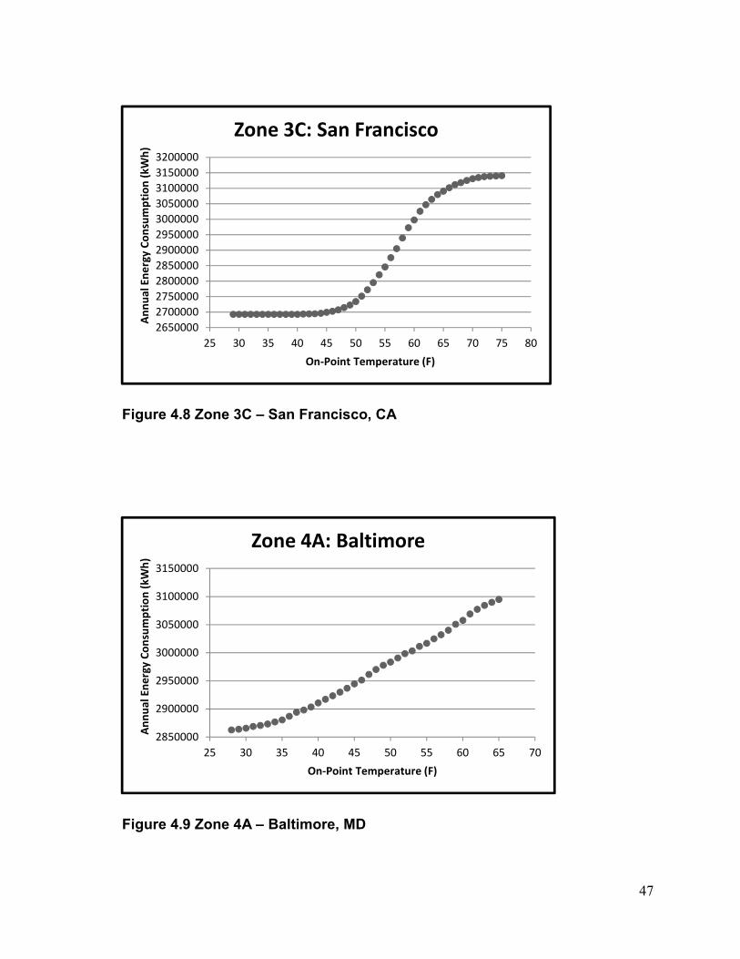
Figure 4.8 Zone 3C – San Francisco, CA

Figure 4.9 Zone 4A – Baltimore, MD

2650000

2700000

2750000

2800000

2850000

2900000

2950000

3000000

3050000

3100000

3150000

3200000

25 30 35 40 45 50 55 60 65 70 75 80

An

nu

al

En

erg

y C

on

sum

pti

on

(k

Wh

)


Zone 3C: San Francisco

2850000

2900000

2950000

3000000

3050000

3100000

3150000

25 30 35 40 45 50 55 60 65 70

An

nu

al

En

erg

y C

on

sum

pti

on

(k

Wh

)


Zone 4A: Baltimore

48

Figure 4.10 Zone 4B – Albuquerque, NM

Figure 4.11 Zone 4C – Seattle, WA

2850000

2900000

2950000

3000000

3050000

3100000

3150000

3200000

25 30 35 40 45 50 55 60 65 70 75 80

An

nu

al

En

erg

y C

on

sum

pti

on

(k

Wh

)


Zone 4B: Albuquerque

2600000

2650000

2700000

2750000

2800000

2850000

2900000

2950000

3000000

3050000

3100000

25 30 35 40 45 50 55 60 65 70 75 80

An

nu

al

En

erg

y C

on

sum

pti

on

(k

Wh

)


Zone 4C: Seattle

49

Figure 4.12 Zone 5A – Chicago, IL

Figure 4.13 Zone 5B – Boulder, CO

2750000

2800000

2850000

2900000

2950000

3000000

3050000

25 30 35 40 45 50 55 60 65 70 75

An

nu

al

En

erg

y C

on

sum

pti

on

(k

Wh

)


Zone 5A: Chicago

2750000

2800000

2850000

2900000

2950000

3000000

3050000

3100000

25 30 35 40 45 50 55 60 65 70 75 80

An

nu

al

En

erg

y C

on

sum

pti

on

(k

Wh

)


Zone 5B: Boulder

50

Figure 4.14 Zone 5C – Vancouver, BC

Figure 4.15 Zone 6A – Minneapolis, MN

2550000

2600000

2650000

2700000

2750000

2800000

2850000

2900000

2950000

3000000

3050000

3100000

25 30 35 40 45 50 55 60 65 70 75 80

An

nu

al

En

erg

y C

on

sum

pti

on

(k

Wh

)


Zone 5C: Vancouver

2750000

2800000

2850000

2900000

2950000

3000000

3050000

25 30 35 40 45 50 55 60 65 70 75

An

nu

al

En

erg

y C

on

sum

pti

on

(k

Wh

)


Zone 6A: Minneapolis

51

Figure 4.16 Zone 6B – Helena, MT

Figure 4.17 Zone 7 – Duluth, MN

2650000

2700000

2750000

2800000

2850000

2900000

2950000

3000000

3050000

25 30 35 40 45 50 55 60 65 70 75 80

An

nu

al

En

erg

y C

on

sum

pti

on

(k

Wh

)


Zone 6B: Helena, MT

2650000

2700000

2750000

2800000

2850000

2900000

2950000

3000000

25 30 35 40 45 50 55 60 65 70 75 80

An

nu

al

En

erg

y C

on

sum

pti

on

(k

Wh

)


Zone 7: Duluth, MN

52

Figure 4.18 Zone 8 – Fairbanks, AK

The curves produced have several shapes. In Figure 4.8 for San Francisco, CA, the

curve of the results were “S” shaped. But, in Figure 4.12 for Chicago, IL, the results are

more linear. On the curves where the slope goes to near zero, in the left of each figure for

lower OA temperatures, this implies the possible optimal low-limit where the slope starts to

increase. But on other curves, seemingly for the colder climates, a minima is not explicit and

those cases must still be further investigated. Ultimately, the goal of this project is to

determine a practical way to estimate the optimal low limit. Calculating the balance point

temperatures for the various locations, and then comparing those results to the simulations’

findings is the next step in characterizing the low limit.

2750000

2800000

2850000

2900000

2950000

3000000

3050000

25 30 35 40 45 50 55 60 65 70 75 80

An

nu

al

En

erg

y C

on

sum

pti

on

(k

Wh

)


Zone 8: Fairbanks, AK

53

CHAPTER V

BALANCE POINT TEMPERATURE

According to ASHRAE Technical Committee (TC) 1.6, the balance point

temperature (TBP, or BPT; in °F or °C) is defined as “The outdoor [dry bulb] temperature at

which a building’s heat loss to the environment is equal to internal heat gains from people,

lights, and equipment… Internal-load dominated structures, like office buildings, may have

balance points so low that the climate never overcomes their internal heat gain” (ASHRAE).

The latter half of this statement implies for some buildings in certain climates they never

require heating due to their high internal heat gains. The low-limit for an air-side economizer

is when the OA air temperature alone allows comfortable conditions within the building to

be maintained without the use of any additional mechanical heating or cooling (Utzinger and

Wasley 1997), so the balance point temperature, a calculated or observed value, seems

similar to the low-limit temperature of a drybulb economizer. But the balance point

temperature is not measurable directly; it must be obtained through years of observation of

a building. Or it may be predicted through calculations using multiple variables that correlate

to a building’s design. Many thermal driving forces exist in a building, including heat

transferred by radiation from the sun, heat released by occupancy, heat generated by lights

and equipment, and conductive transfer of energy across the building enclosure. These

energy flows can be evaluated under quasi-steady conditions, but a transient analysis that

also accounts for heat storage and release from the masses within the building would better

characterize the actual buildings’ performance in that particular climate.

The balance point temperature thus represents a practical energy balance of all of the

54

aforementioned variables except the “thermal masses.” Mathematically the balance point

temperature, �� , is a combination of these variables (Utzinger et. al Wasley),

�� = �� − � �� (5.1)

where �� is the thermostat’s setpoint temperature and �� is calculated from

� �� =

�� ! + �#$

%& �$'!

. (5.2)

�� and �� have units of °F or °C. In Equation 5.2 )*+,, defined per unit floor

area, is the buildings internal heat gain rate due to occupancy. )�-. is the rate of solar heat

gain per unit floor area. /&�.0, is the overall heat transfer across the building enclosure per

unit floor area and per degree temperature difference. These three variables are constantly

changing as they are affected by occupancy, time of day and year, weather conditions, and

air exchange rates; /&�.0, changes based on the current infiltration and ventilation rate.

Because these variables change, the balance point temperature does vary somewhat with

time for a particular building and climate. When only one balance point temperature is stated,

which is the norm, it represents a compilation or possibly only one set of conditions such as

those for the “worst case.” So the method for determining the low-limit presented here

should be considered as a refined starting point, and the value should be adjusted after

observing the operation of the particular HVAC system over time and under various

conditions.

The internal heat gains can be separated into their sensible and latent components.

55

Humans emit moisture at varying rates due to their different levels of activity. Typically,

one of two methods is used to determine the heat gains of occupancy. The first method is a

lookup-table in the Fundamentals volume of the ASHRAE Handbook (ASHRAE 2013). The

chapter “Nonresidential Cooling and Heating Load Calculations” provides a table that gives

rates at which heat and moisture are emitted based on a human’s different level of activity.

The second, more fundamental method is given in ASHRAE Standard 55-2013 and uses

metabolic rates. Metabolic rate, as defined in ASHRAE Standard 55-2013, is “the rate of

transformation of chemical energy into heat and mechanical work by metabolic activities

within an organism, usually expressed in terms of unit area of the total body surface”

(ASHRAE Standard 55-2013).

Another part of the buildings’ internal heat gains is from lights and equipment. For

lights, the electrical energy consumed by each fixture is ultimately equivalent to the rate of

heat dissipated; some of the heat gain becomes a load immediately while the remainder is

stored in masses and then released later. Similarly for equipment, the heat released is equal

to the energy each piece of equipment consumes, but with certain equipment, such as steam

tables and coffee pots, there’s also a latent component; the building’s masses can store and

release moisture as well as the sensible heat. As previously noted, )*+, is the total internal

heat gain per unit floor area, and is

�� ! = ��1#�$1 + �$�! � + �1�%�� (5.3)

where )�2-�.2 is the heat gain from people occupying the building per unit floor area,

).*,+�� is the heat gain from the lights used during occupancy per unit floor area, and

)234*� is the heat gain from equipment per unit floor area. These values can be characterized

56

as steady-state or transient. The DOE-2 based program eQUEST uses the “quasi-steady”

approach – hourly-averaged values are found, and energy storage and release is characterized

with relatively simple time-lag factors that vary with the construction materials used.

The next variable in the balance point temperature equation is the solar heat

gain, )�-.�5 that can also be described by

�#$ = 6789/��988; . (5.4)

)�-. is, of course, transient. But for the ultimate purpose of this study, a simplified way to

characterize or gather the solar heat gain was needed. Such will be presented later in this

thesis.

The overall building heat transfer coefficient has multiple components too (Utzinger

et. al 2011 Wasley):

%& <9�= = %& >?99 + %& ;88� + %& =9@= + %& =;A� + %& B�A (5.5)

where /&CDEE represents the floor area-averaged heat transfer coefficient through the buildings

walls. It is determined from

%& >?99 = (%>?99 ∗ �>?99)/��988; (5.6)

where /CDEE is the overall heat transfer coefficient for the exterior walls of the building.

Second, ICDEE is the total wall surface area and I�EJJK is the overall building floor area. This

is the overall U-value for the entire building; the equations are not normally applied to floors

individually. The other components of equation 5.5 are /&KJJ� , /&LEML , and /&LKN� ;

determining all three follow the same concept of the building heat transfer rate through the

57

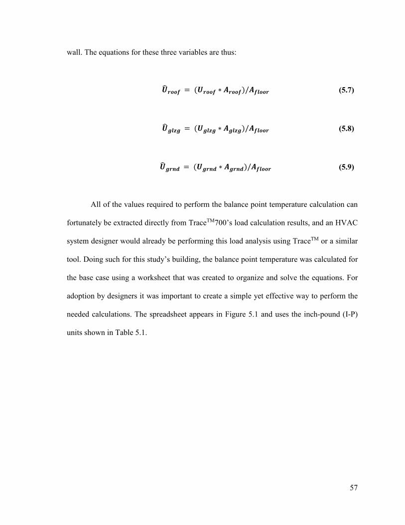
wall. The equations for these three variables are thus:

%& ;88� = (%;88� ∗ �;88�)/��988; (5.7)

%& =9@= = (%=9@= ∗ �=9@=)/��988; (5.8)

%& =;A� = (%=;A� ∗ �=;A�)/��988; (5.9)

All of the values required to perform the balance point temperature calculation can

fortunately be extracted directly from TraceTM700’s load calculation results, and an HVAC

system designer would already be performing this load analysis using TraceTM or a similar

tool. Doing such for this study’s building, the balance point temperature was calculated for

the base case using a worksheet that was created to organize and solve the equations. For

adoption by designers it was important to create a simple yet effective way to perform the

needed calculations. The spreadsheet appears in Figure 5.1 and uses the inch-pound (I-P)

units shown in Table 5.1.

58

Table 5.1 Building Balance Point Temperature Worksheet Units

Variable Units

%>?99 Btu/Hr/sf2/°F

�>?99 sf2

��988; sf2

%;88� Btu/Hr/ sf2/°F

�;88� sf2

%=9@= Btu/Hr/ sf2/°F

�=9@= sf2

%=;A� Btu/Hr/LF/°F

�=;A� sf2

%& >?99 Btu/Hr/°F/ sf2

%& ;88� Btu/Hr/°F/ sf2

%& =9@= Btu/Hr/°F/ sf2

%& =;A� Btu/Hr/°F/ sf2

%& <9�= Btu/Hr/°F/ sf2

6��8�9� Btu/Hr

69�=O Btu/Hr

6�6P�� Btu/Hr

��1#�$1 Btu/Hr/ sf2

�$�! � Btu/Hr/ sf2

�1�%�� Btu/Hr/ sf2

�� ! Btu/Hr/ sf2

6789 Btu/Hr

�#$ Btu/Hr/ sf2

�� °F

� �� °F

�� °F

59

Fig

ure

5.1

: B

uil

din

g B

ala

nc

e P

oin

t T

em

pera

ture

Wo

rks

hee

t

60

When using TraceTM700, its resulting “System Checksums” report contains the majority of

the data required to calculate the building’s balance point temperature. An example, using

this study’s base case, follows.

The first value needed from the System Checksums report is the floor square footage,

Afloor. Figure 5.2 shows where to find this value on the report. The needed U-values were

determined based on the construction of the building.

61

Figure 5.2 Collecting floor area square footage from a Trane Trace® System

Checksums report

Figure 5.3 indicates where to enter the U-Values and the floor area, on the template.

62

Figure 5.3 Building balance point temperature worksheet with the example’s

U-values and floor area entered

The next step is to gather the total wall area, roof area, and glazing area from the

System Checksums report. This information can be found on the System Checksums report

as seen in Figure 5.4. Figure 5.5 shows the values filled in on the worksheet.

108,09 108,09 108,09 108,09

0.052516 0.035693 0.505 0.490998

108,09 108,09 108,09

108,09

63

Figure 5.4 Collecting wall, roof, and glazing areas from the System

Checksums report.

64

Figure 5.5 Building balance point temperature worksheet with the wall, roof,

and glazing areas added

While almost all needed values can be found from earlier input data or the System

Checksums report, a couple values cannot. Those two values are the perimeter of the

building and the infiltration and ventilation heat transfer rate. The perimeter of the building

is a simple calculation using the exterior dimensions obtained from the architectural plans.

The building’s air exchange heat transfer rate can be challenging to determine. For the

ultimate practical result of this project – a design method for finding the low-limit -- a

conservative estimate was used. The value chosen for this building’s air exchange heat

transfer rate was 0.13 Btu/hr/ft2/°F.

108,09 108,09 108,09 108,09

0.052516 0.035693 0.505 0.490998

108,09 108,09 108,09

108,09

30,090 30,582 18,084

65

With these values determined, they can then be added to the Building Balance Point

Temperature Worksheet as shown in Figure 5.6.

Figure 5.6 Building balance point temperature worksheet with the building’s

perimeter and air exchange heat transfer coefficient added

108,09 108,09 108,09 108,09

0.052516 0.035693 0.505 0.490998

108,09 108,09 108,09

108,09

30,090 30,582 18,084 994

0.13

66

The next step is to collect the internal heat gain rates. Again, the internal heat gain

rates for the building are those from people, lights, and equipment. Figure 5.7 shows where

those values are found on the System Checksums report of Trane Trace®.

Figure 5.7 Collecting internal heat gain rates from the System Checksums

report

67

The last value needed for the worksheet is the solar heat gain rate. As with most of

the other data values, the solar heat gain rate can fortunately be found on the System

Checksums report. Figure 5.8 gives the location of the solar heat gain rate on the report.

Figure 5.8 Collecting the solar heat gain rate from the System Checksums

report

68

The Building Balance Point Temperature Worksheet, now complete for the base case

of this study, appears in Figure 5.9.

Figure 5.9 Building balance point temperature worksheet with the internal and

solar heat gains added

108,09 108,09 108,09 108,09

0.052516 0.035693 0.505 0.490998

108,09 108,09 108,09

108,09

30,090 30,582 18,084 994

0.13

305,880 294,128 355,022

253,279

69

The next step, via cell formulas in the spreadsheet, is the calculation using all the

data collected. The building heat transfer rate calculation is separated into heat transfer

through walls, roof, glazing, ground, and air exchange. The normalized heat transfer rate

through the building walls is:

%& >?99 = (%>?99 ∗ �>?99)/��988; (5.10)

Figure 5.10 gives the results for this example.

Figure 5.10 Building balance point temperature worksheet’s wall heat rate

calculation for the base case

The roof’s heat transfer rate is:

%& ;88� = (%;88� ∗ �;88�)/��988; (5.11)

Figure 5.11 shows the results for the base case’s roof.

0.052516

30,090

108,096

0.014619

Btu/Hr/ft2/°F

ft2

ft2

Btu/Hr/°F/ ft2

70

Figure 5.11 Building balance point temperature worksheet roof heat rate


The next two parts of the worksheet pertain to the glazing and the ground or slab:

%& =9@= = (%=9@= ∗ �=9@=)/��988; (5.12)

%& =;A� = (%=;A� ∗ �=;A�)/��988; (5.13)

Similar to that for the walls and the roof Figures 5.12 and 5.13 show the calculations for

glazings and the ground contact.

0.035693

30,582

108,096

0.010098

Btu/Hr/ft2/°F

ft2

ft2

Btu/Hr/°F/ ft2

71

Figure 5.12 Building balance point temperature worksheet’s glazing heat rate


Figure 5.13 Building balance point temperature worksheet’s ground heat rate


0.505

18,084

108,096

0.84484

Btu/Hr/ft2/°F

ft2

ft2

Btu/Hr/°F/ ft2

0.490998

994

108,096

0.004515

Btu/Hr/ft/°F

ft

ft2

Btu/Hr/°F/ ft2

72

Finally, the last needed value is the normalized ventilation heat transfer rate, and it

is already in a directly useable form, /&Q�N� = 0.13.

With the needed data calculated, the overall building heat transfer rate is:

%& <9�= = %& >?99 + %& ;88� + %& =9@= + %& =;A� + %& B�A (5.14)

The total for /&UE�L for the base case is 0.243716 BTU/h∙ft2∙°F.

The next portion of the Building Balance Point Temperature calculation produces

the overall internal heat gains for the building. The first component of this value is the

internal heat gain due to occupancy:

��8�9� = 6��8�9�/��988; (5.15)

Similarly, the internal heat gains due to lights and equipment are needed:

�9�=O 7 = 69�=O 7/��988; (5.16)

��6P�� = 6�6P��/��988; (5.17)

With these data, the internal heat gains are determined within the worksheet, as shown in

Figures 5.14 through 5.16.

73

Figure 5.14 Building balance point temperature worksheet’s occupancy heat

transfer rate, calculation for the base case

Figure 5.15 Building balance point temperature worksheet’s lighting heat

transfer rate calculation for the base case

108,096

305,880

2.83

ft2

Btu/Hr

Btu/Hr/ ft2

2.72

294,128

108,096 ft2

Btu/Hr

Btu/Hr/ ft2

74

Figure 5.16 Building balance point temperature worksheet’s equipment heat


After completion of the three internal heat gain calculations, the overall building

internal heat gain is:

�� ! = ��8�9� + �9�=O + ��6P�� (5.18)

The calculations in the third section of the Building Balance Point Temperature

Worksheet, for the solar energy, are similar to that for the internal heat gains. This quick

calculation of the solar heat gains, that are dependent on the location of the building, is:

�#$ = 6789/��988; (5.19)

For the base case, the result of solving the equation is shown in Figure 5.17.

3.28

355,022

108,096 ft2

Btu/Hr

Btu/Hr/ ft2

75

Figure 5.17 Building balance point temperature worksheet’s solar heat


The thermostat’s setpoint temperature for cooling mode used in the modeling

software was next needed for the final section’s calculations. With it, the temperature

difference due to the internal and solar heat gains, TE-Flow, is found:

�1VW$#X =

�� ! + �#$

%& �$'!

(5.20)

Once this value for the temperature has been calculated, the balance point temperature for

the building and its particular geographic location can be determined:

�� = �� − �1VW$#X (5.21)

The worksheet’s, balance point temperature calculation, for the base case, is given in Figure

5.18.

2.34

253,279

108,096 ft2

Btu/Hr

Btu/Hr/ ft2

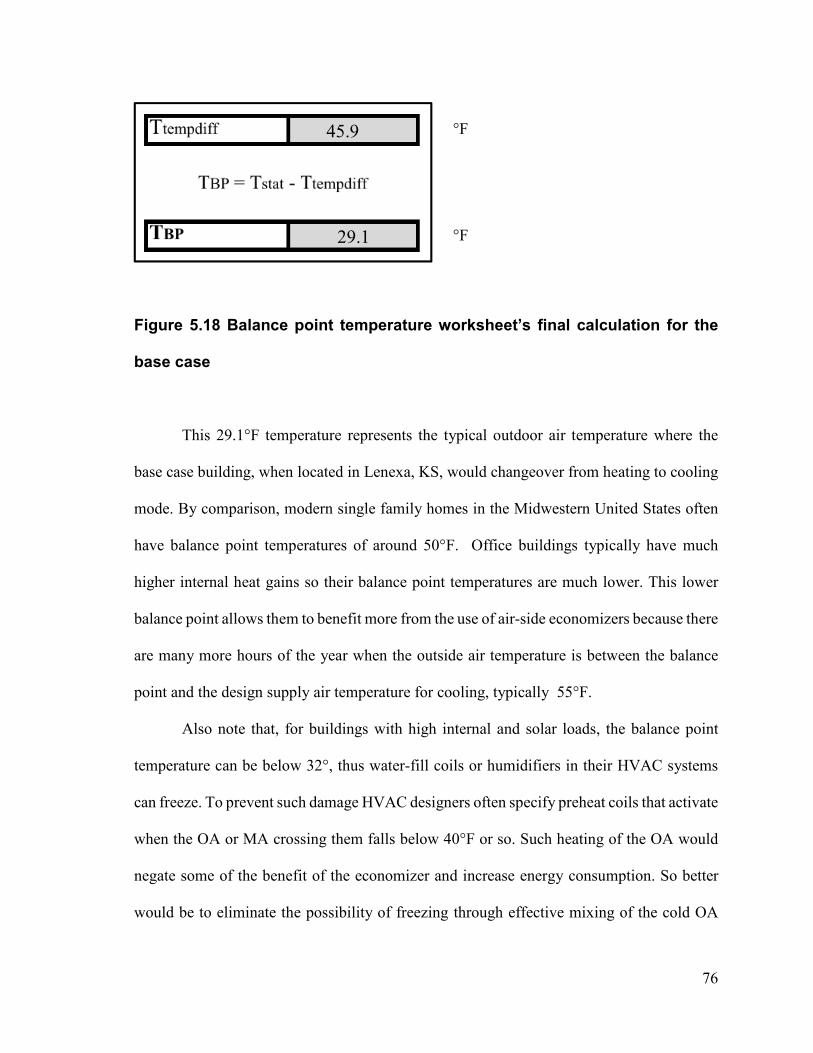
76

Figure 5.18 Balance point temperature worksheet’s final calculation for the

base case

This 29.1°F temperature represents the typical outdoor air temperature where the

base case building, when located in Lenexa, KS, would changeover from heating to cooling

mode. By comparison, modern single family homes in the Midwestern United States often

have balance point temperatures of around 50°F. Office buildings typically have much

higher internal heat gains so their balance point temperatures are much lower. This lower

balance point allows them to benefit more from the use of air-side economizers because there

are many more hours of the year when the outside air temperature is between the balance

point and the design supply air temperature for cooling, typically 55°F.

Also note that, for buildings with high internal and solar loads, the balance point

temperature can be below 32°, thus water-fill coils or humidifiers in their HVAC systems

can freeze. To prevent such damage HVAC designers often specify preheat coils that activate

when the OA or MA crossing them falls below 40°F or so. Such heating of the OA would

negate some of the benefit of the economizer and increase energy consumption. So better

would be to eliminate the possibility of freezing through effective mixing of the cold OA

45.9

29.1

°F

°F

77

and the warm CA, or to fully eliminate the use of water downstream of the OA intake during

cold conditions. Some steam heating coils are fully self-draining, for example.

78

CHAPTER VI

ECONOMIZER SET POINT ANALYSIS

An air-side economizers’ high limit has typically been set to 68 to 70°F, with toward

the former in humid climates and toward the latter in drier. The low-limit should vary with

climate zone, however, due to the weather’s significant effect on a building’s cooling load

as described previously. Recently, the selection of the high limit has become more refined

as shown through ASHRAE Standard 90.1-2013 (ASHRAE 2013). Designers need similar

guidance for the low-limit. Up to now no values for the low limit of the airside economizer

have been suggested in the Standard. Part of the difficulty in predefining the low limit is the

range of the economizer performance within each climate zone. A standard designer’s rule-

of-thumb has been to specify the low-limit as the balance point temperature, but often not

lower than 40°F to prevent freezing of coils.

In the previous chapter, the balance point temperature was introduced and is the OA

temperature where no heating or cooling is needed; the heat gains of the building equal the

heat losses. Cooling, mechanically-produced or otherwise, is required when the OA

temperature increases above the balance point temperature. At that point, when provided, an

air-side economizer would activate to provide that cooling until its limit of effectiveness is

reached. The equation for estimating the balance point temperature includes the effect of

climate, but many other factors are constants. This allows the balance point temperature to

be predicted for specific climate zones. To observe the relation of the low limit to the balance

point temperature, calculations were thus made for each climate zone. The determined

temperatures can be found in Table 6.1.

79

Table 6.1 Calculated balance point temperature for each climate zone for the

base case building

Climate Zone

Location Balance Point

Temperature (°F (°C))

Base Case Lenexa, KS 29.1 (-1.6)

1A Miami, FL 29.7 (-1.3)

2A Houston, TX 30.0 (-1.1)

2B Phoenix, AZ 29.3 (-1.5)

3A Atlanta, GA 29.2 (-1.6)

3B Los Angeles, CA 28.9 (-1.7)

3C San Francisco, CA 28.8 (-1.8)

4A Baltimore, MD 29.7 (-1.3)

4B Albuquerque, NM 29.2 (-1.6)

4C Seattle, WA 28.9 (-1.7)

5A Chicago, IL 29.4 (-1.4)

5B Boulder, CO 28.4 (-2.0)

5C Vancouver, BC 28.6 (-1.9)

6A Minneapolis, MN 29.3 (-1.5)

6B Helena, MT 28.4 (-2.0)

7 Duluth, MN 28.8 (-1.8)

8 Fairbanks, AK 28.3 (-2.1)

80

Chapter IV examined how the energy consumption varies with the low limit. The

remainder of this chapter shows how the balance point temperature relates to the low limit.

In addition, the energy consumption for the high-limit selected is shown via point “A” on

the following figures. Point “B” is the energy consumption with a 55°F (12.8°C) low limit

and thus no free cooling. Point “C” shows the energy consumption with the low limit equal

to the balance point temperature. Range “D” represents the savings by using an economizer

but with no free cooling. Range “E” is the additional savings by operating the economizer

with the free cooling. Range “F” shows the total savings when utilizing the air-side

economizer fully from the low-limit equal to the balance point. Figure 6.1 shows these points

and ranges for the base case in Lenexa, KS. Table 6.2 provides the numerical values for

them. Figures 6.2 through 6.17 and Tables 6.3 through 6.18, for the base case building and

each of the different climate zones, present their energy consumption and savings potential.

81

Figure 6.1 Results for the base case in Lenexa, KS with points and ranges of

interest

Table 6.2 Base case energy consumption or savings (kWh).

Point or

Range

Annual Energy Consumption

or Savings

A 3,099,700

B 3,023,500

C 2,894,900

D 76,200

E 128,600

F 204,800

82

Figure 6.2 Results for Zone 1A in Miami, FL with points and ranges of

interest

Table 6.3 Zone 1A energy consumption or savings (kWh).

Point or

Range


or Savings

A 3,446,400

B 3,426,700

C 3,421,200

D 19,700

E 5,500

F 25,200

83

Figure 6.3 Results for Zone 2A in Houston, TX with points and ranges of

interest


Point or

Range


or Savings

A 3,320,100

B 3,258,800

C 3,195,700

D 61,300

E 63,100

F 124,400

84

Figure 6.4 Results for Zone 2B in Phoenix, AZ with points and ranges of

interest

Table 6.5 Zone 2B energy consumption or savings (kWh).

Point or

Range


or Savings

A 3,344,700

B 3,230,300

C 3,179,200

D 114,400

E 51,100

F 165,500

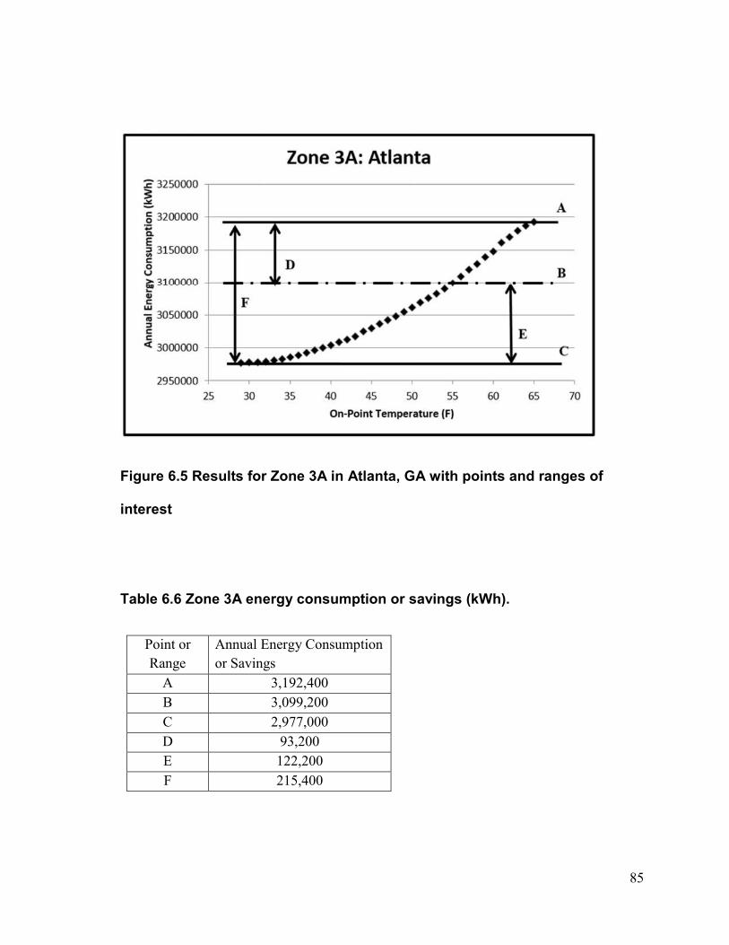
85

Figure 6.5 Results for Zone 3A in Atlanta, GA with points and ranges of

interest


Point or

Range


or Savings

A 3,192,400

B 3,099,200

C 2,977,000

D 93,200

E 122,200

F 215,400

86

Figure 6.6 Results for Zone 3B in Los Angeles, CA with points and ranges of

interest


Point or

Range


or Savings

A 3,211,200

B 2,956,000

C 2,925,000

D 255,200

E 31,000

F 286,200

87

Figure 6.7 Results for Zone 3C in San Francisco, CA with points and ranges

of interest

Table 6.8 Zone 3C energy consumption or savings (kWh).

Point or

Range


or Savings

A 3,141,000

B 2,846,500

C 2,693,400

D 294,500

E 153,100

F 447,600

88

Figure 6.8 Results for Zone 4A in Baltimore, MD with points and ranges of

interest

Table 6.9 Zone 4A energy consumption and savings (kWh).

Point or

Range


or Savings

A 3,095,100

B 3,016,800

C 2,869,500

D 78,300

E 150,900

F 229,200

89

Figure 6.9 Results for Zone 4B in Albuquerque, NM with points and ranges of

interest


Point or

Range


or Savings

A 3,178,300

B 3,049,200

C 2,872,600

D 129,100

E 176,600

F 305,700

90

Figure 6.10 Results for Zone 4C in Seattle, WA with points and ranges of

interest


Point or

Range


or Savings

A 3,038,100

B 2,866,500

C 2,628,700

D 171,600

E 237,800

F 409,400

91

Figure 6.11 Results for Zone 5A in Chicago, IL with points and ranges of

interest


Point or

Range


or Savings

A 3,015,600

B 2,933,600

C 2,778,800

D 82,000

E 154,800

F 236,800

92

Figure 6.12 Results for Zone 5B in Boulder, CO with points and ranges of

interest


Point or

Range


or Savings

A 3,072,800

B 2,959,500

C 2,775,000

D 113,300

E 184,500

F 297,800

93

Figure 6.13 Results for Zone 5C in Vancouver, BC with points and ranges of

interest


Point or

Range


or Savings

A 3,029,500

B 2,865,700

C 2,602,300

D 163,800

E 263,400

F 427,200

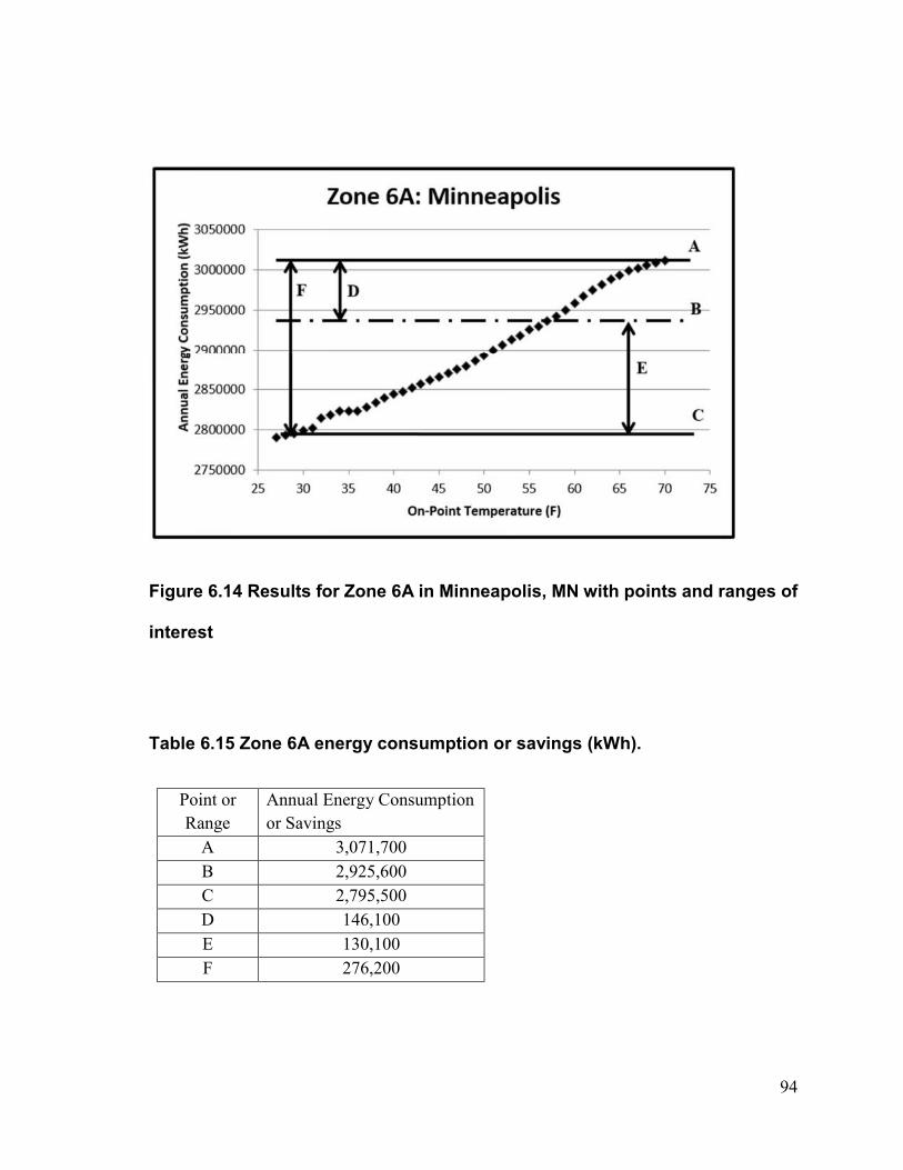
94

Figure 6.14 Results for Zone 6A in Minneapolis, MN with points and ranges of

interest


Point or

Range


or Savings

A 3,071,700

B 2,925,600

C 2,795,500

D 146,100

E 130,100

F 276,200

95

Figure 6.15 Results for Zone 6B in Helena, MT with points and ranges of

interest


Point or

Range


or Savings

A 2,998,000

B 2,879,300

C 2,675,200

D 118,700

E 204,100

F 322,800

96

Figure 6.16 Results for Zone 7 in Duluth, MN with points and ranges of interest

Table 6.17 Zone 7 energy consumption or savings (kWh).

Point or

Range


or Savings

A 2,954,300

B 2,853,600

C 2,688,000

D 100,700

E 165,600

F 266,300

97

Figure 6.17 Results for Zone 8 in Fairbanks, AK with points and ranges of

interest

Table 6.18 Zone 8 energy consumption or savings (kWh).

Point or

Range


or Savings

A 3,019,600

B 2,921,500

C 2,778,200

D 98,100

E 143,300

F 241,400

98

This chapter’s figures and tables indicate that in almost all cases there is a clear low-

limit. The calculated balance point temperature for each location corresponded to where the

slope of the energy consumption variation became near zero. These results verify the rule-

of-thumb used for decades that the low-limit for an air-side economizer should be the

balance point temperature of the building.

The balance point temperatures across the climate zones were similar for this

building, which was an interesting finding. From Chapter V the largest variable by climate

zone was the instantaneous solar load. However, the annual total solar load didn’t vary

enough across the climate zones to have a large effect on the balance point temperature

which is an annual-average value.

Based on the aforementioned cases, a reason that most air-side economizers are not

functioning at their highest potential is becoming clear. Designers are specifying or installers

are setting too high low-limit setpoints; significant savings can be had by using much lower

low-limits that are equal to the balance point temperatures of the buildings, but freeze

protection must be included.

99

CHAPTER VII

CONCLUSIONS AND RECOMMENDATIONS

The purpose of this research study was to examine drybulb air-side economizer low-

limits’ effect on energy consumption for an office building in many North American

climates. The base case selected was a real four-story commercial office building, of typical

modern design and construction, in Lenexa, KS. This study used two different modeling

programs for the HVAC load and energy simulations -- TraceTM700 and eQUEST. As

similar inputs as possible were used with each program, and, for the base case, the results

were compared to several years’ worth of actual utility data to calibrate the model. Both

programs were then used to perform simulations in 16 typical climates of North America.

eQUEST, being a more robust program, was used to perform the many simulations needed

to evaluate the annual energy consumption when the air-side economizer was activated and

its low-limit temperature varied for each of the weather sites. The high-limit temperature

was held constant. The simulations’ results were then plotted for each of the climate zones.

Many of the resulting curves of annual cooling energy use, for each climate zone, had an

obvious outside air temperature setting for the low-limit where the reduction in energy

consumption became close to zero. The next step in this study was to find a way to calculate

this optimal low-limit temperature so that HVAC designers can specify the value. The

historical rule-of-thumb is that the low-limit is the balance point temperature. However, the

annual-average balance point temperature is not easily calculated -- this was observed to be

due to the transient solar heat gain component. The ultimate goal of this project was to create

a practical way to perform the calculation. Using the results from a TraceTM700 loads’

100

prediction allowed that to be possible, and performing these load calculations are already

routinely done as part of HVAC designs. A Building Balance Point Temperature worksheet

was created in this project. The worksheet allows the engineer to enter data directly from a

TraceTM700 “System Checksums” report or other similar transient HVAC load calculation

programs. When utilizing these loads calculations programs it’s important for the designer

to select an algorithm that uses transient hour-by-hour calculations, with appropriate weather

data, so that the buildings’ solar and other thermal characteristics are adequately modeled to

capture the annual, rather than steady-state “worst case” performance.

In this study, after calculating the balance point temperatures for each of the various

climate zones, these values were compared to the curves of annual energy consumption. This

comparison verified that the optimal low-limits were consistent with the balance point

temperatures calculated. Comparing the results confirmed the decade’s old rule-of-thumb to

be valid, at least for the building and climates studied. This study resulted in a practical

balance point temperature worksheet that allows an HVAC designer to calculate that optimal

economizer low-limit. Furthermore, it was found that there is a high level of additional

energy and cost savings associated with defining this low-limit lower than a commonly-

assumed 40°F (4.4°C) or so. This 40°F assumption likely is from a desire to prevent freezing

of water-filled coils in the air handling systems.

Recommendations

Currently, ASHRAE Standard 90.1-2013 gives requirements for airside economizers

but with no mention of the low-limit. This study shows that ASHRAE Standard 90.1-2013

needs to include the optimal low-limit. The requirement for the dry-bulb airside

101

economizers’ sensors accuracy needs revision too. Currently ASHRAE Standard 90.1-2013

states “Outdoor air, return air, mixed air, and supply air sensors shall be calibrated within

the following accuracies: a. Dry-bulb and wet-bulb temperatures shall be accurate to ±2°F

over the range of 40°F to 80°F…” (ASHRAE 90.1-2013). This study indicates that optimal

low-limits can be 30°F or lower, so the sensors’ accuracy should be assured at those reduced

temperatures too. A study of the high-limit requirements already in place in ASHRAE

Standard 90.1-2013 is also recommended.

If airside economizers’ performance were optimized, the energy savings would be

vast; expanding the use of the airside economizers to all appropriate buildings is needed too.

With buildings now consuming 40% of the primary energy in the U.S., reducing it through

expanded use of optimized air-side economizers can noticeably improve energy security and

decrease greenhouse gas emissions.

102

APPENDIX

TRANE TRACE DATA

106

References

ASHRAE. 2013a. ANSI/ASHRAE/IES Standard 90.1-2013. Energy Standard for Buildings

Except Low-rise Residential Buildings. I-P ed. Atlanta: Print.

ASHRAE. 2013b. ANSI/ASHRAE/ASHE Standard 62.1-2013: Ventilation for Acceptable

Indoor Air Quality. Atlanta: Print.

ASHRAE. 2013c. ANSI/ASHRAE/ASHE Standard 55-2013: Thermal Environmental

Conditions for Human Occupancy. Atlanta: Print.

ASHRAE. 2013d. ASHRAE Handbook, Fundamentals volume. Atlanta, GA: American

Society of Heating, Refrigerating and Air Conditioning Engineers.

eQuest. 1999. eQuest energy calculation software and user manuals.

http://www.doe2.com/equest/.

Taylor, S.T., and Cheng, C.H. “Economizer High Limit Controls and Why Enthalpy

Economizers Don’t Work,” (TECHNICAL FEATURE) ASHRAE Journal, (2010,

Nov. 1) Print.

Trane Engineers Newsletter. “Keeping Cool with Outside Air... Airside Economizers.” No.

35 (2013, Jan. 1): pp. 1–8.

Utzinger, Michael, and James H. Wasley. “Building Balance Point.” Vital Signs -

University of Wisconsin-Milwaukee, (2001). Print.

107

Bibliography

Brandemuehl, M. J., and J. E. Braun. “The Impact of Demand-Controlled and Economizer

Ventilation Strategies on Energy Use in Buildings.” ASHRAE Transactions 105,

no. 2 (1999).

Emmerich, Steven J., Andrew K. Persily, W. Stuart Dols, and James W. Axley. NISTIR

7062 (n.d.): Oct. 2003.

Haines, Roger W., and D. Hittle. Control Systems for Heating, Ventilating, and Air

Conditioning. New York: Van Nostrand Reinhold, 1993. Print.

Rabun, J. Stanley., and Richard Miles Kelso. Building Evaluation for Adaptive Reuse and

Preservation. Hoboken, NJ: Wiley, 2009. Print.

Rock, B.A., and C. Wu. “Performance of Fixed, Air-Side Economizer, and Neural

Network Demand-Controlled Ventilation in CAV Systems.” ASHRAE Transactions

104, no. 2 (1998): pp.234–245.

Sorell, Vali. “OA economizers for data centers (Outside Air) (Technical report).” ASHRAE

Journal (2007, Dec. 1): pp. 32–37.

Taras, Michael F. “Is Economizer Cycle Justified for AC Applications?” ASHRAE

Journal (2005, July 1): pp. 38–44.

Zhou, J., G. Wei, D. Turner, and D. Claridge. 2008. “Airside Economizer—Comparing

Differing Control Strategies and Common Misconceptions.” Project presentation,

http://repository.tamu.edu/handle/1969.1/90822.

Airside Economizer Low Limit Effect on Energy and Thermal ...

Documents

Transcript of Airside Economizer Low Limit Effect on Energy and Thermal ...