158

ADVANCED RAY-BASED SYNTHETIC SEISMOGRAMS

T. Kaschwich, I. Lecomte, H. Gjøystdal, E. Iversen, and M. Tygel

email: tina@norsar.nokeywords: Modeling, Kirchhoff-type

ABSTRACT

Ray-based seismic modeling methods can be applied at various stages of the exploration and produc-tion process, e.g., for comparison, simulation or representation of seismic data, to assess the ambiguityof interpretation or to make predictions. Ray tracing in its standard forms is not always able to producecomplete synthetic seismograms, as may be required for processing tests. Standard reflection-basedmodeling gives good results in many cases, but could fail for some complex structures. For instance, inthe presence of sharp edges and ripples on the modeled reflector or in the vicinity of caustics classicaldynamic ray tracing (DRT) does not give reliable amplitude values. Therefore, we propose alternativeapproaches where reflection modeling is not used. Instead we use an optimized ray-based approachto calculate various types of Green’s functions (GF), e.g., amplitudes and traveltimes, which will beapplied within tailored modeling schemes, such as Kirchhoff modeling and modeling by demigration.Furthermore, we adapt the classical modeling by demigration approach using an alternative PSDMsimulator. Even a simple two-layer model reveals the weaknesses of the standard ray tracing, anddemonstrates on the contrary that the computed seismograms for the alternative methods are morecomplete and significantly improved. Finally, we document the applicability of all methods using amore complex model.

INTRODUCTION

Ray-based seismic modeling methods can be applied at various stages of the exploration and productionprocess. The standard ray method has several advantages, e.g., computational efficiency. In addition raytracing has an event-oriented nature, which means that specific arrivals of elementary waves (e.g., transmit-ted P and S waves, primary PP and PS reflected waves for selected horizons, multiples, etc.) can be labeledin synthetic seismograms or in computed sets of Green‘s function attributes. In early applications the focuswas mostly on the calculation of raypaths and traveltimes (kinematic ray tracing), but throughout the sev-enties and eighties, numerical techniques were developed within dynamic ray tracing (DRT), giving fairlyreliable estimates of amplitudes of both P and S waves. These amplitudes have a firm theoretical basis,being a high-frequency solution of the elastic wave equation (zeroth-order ray theory; Cervený, 2001). Theray attributes become reasonably stable if velocity gradients and interface normals vary smoothly withinthe seismic wavelength. Comparisons with more complete (and much more time-consuming) techniques,like finite-difference schemes (FD), show that DRT-based theoretical seismograms can be very qualified ifthe model is prepared with the necessary smoothness.The main weakness of the ray method applied to complex geological structures is due to the fact that thecalculations along each ray is "super-local", that is, quite independent of the neighboring rays. One singleray "sees" only the velocity and interface behavior exactly along the raypath, and thus the stability acrossthe rays depends on the assumption that these parameters are fairly representative for neighboring rays (atleast within the Fresnel zone). Classical DRT traces continuous rays from source to receiver (two-point raytracing), e.g., making use of the so-called shooting technique, adjusting the take-off direction of the ray andre-tracing until the ray hits sufficiently close to the receiver. For complex 3D models this technique may be

Annual WIT report 2009 159

very time consuming and can typically miss events (rays) in regions with large geometrical spreading. Asan alternative, Vinje et al. (1993, 1996a,b); Gjøystdal et al. (2002, 2007) developed the wavefront construc-tion method (WFC), which is a more robust ray tracing technique adapting the ray density to the modeland interpolating the ray attributes. The reason for enhanced robustness lies in the fact that a continuousrepresentation of the wavefront, with sufficiently dense sampling of ray points and slowness vectors, isestablished by interpolation after each time step. In this way, the sampling of parameters influencing thecalculation of traveltimes, amplitudes, etc., is adapted to the complexity of the model of elastic parameters.Quite recently, the wavefront construction method has been further developed to include anisotropy (Mis-pel and Williamson, 2001; Gibson et al., 2005; Iversen, 2004). However, this method only partly solves theproblem of lack of ray penetration into shadow zones.In this paper we demonstrate new seismic modeling techniques that have been specifically developed tomeet the demands of complex modeling in the petroleum industry. Given the objective of improving theapplicability of the standard ray method, we define each ray-based process as an element of a system,which, as a composite process, is able to obtain better results than the ray-based process applied alone.They are, however, still firmly based on the basic WFC/DRT methodology, i.e., high-frequency approxi-mation of the wave equation. We first demonstrate the pure DRT method and illustrate how some of thebasic weaknesses can be reduced by applying the "DRT engine" in different ways, giving a more robustand realistic behavior. Therefore, we have implemented the Kirchhoff-Helmholtz (KH) modeling tech-nique and the modeling-by-demigration approach.The KH modeling technique should give more accurate and realistic reflection seismograms than thoseobtained by classical ray tracing in case of complex geological structures, because the KH integral consistsof an integration along the reflector. By this, one sums the Huygens secondary-source contributions to thewavefield attached to the reflector at the observation point (Tygel et al., 1994, 2000).Demigration itself can be defined as the inverse of migration (Hubral et al., 1996; Tygel et al., 1996; Santoset al., 2000). This involves nothing more than the formulation of a reflection imaging process by whichone can return from a true amplitude depth migrated section to the original time section. Modeling bydemigration represents a special implementation of the demigration concept, where the input is no longerstandard migrated data but artificially migrated target geological structure(s) defined by the user. In thispaper, the artificially migrated inputs are computed by employing both the standard approach (Tygel et al.,1996; Santos et al., 2000) and the PSDM simulator approach of NORSAR (SimPLI technology, Lecomte,2006, 2008a). This PSDM simulator is used to directly produce simulated prestack depth migrated imagesof a given target, without generating synthetic traces and processing them (Lecomte et al., 2003; Lecomte,2004; Lecomte and Pochon-Guerin, 2005).

METHODOLOGY

In this section, we give an overview and brief introduction to the methodology to be applied. For allmethods Green’s functions (Aki and Richards, 1980) are needed and as mentioned above, calculated byray tracing. The Green‘s functions (GF) represent the wave field propagation between two points in agiven velocity model. However, in our case, in practice, one of these points is a source or receiver of aseismic survey, and as such often near the surface (not true for the VSP case). Besides the traveltimes,ray tracing calculates amplitudes and other parameters (e.g., polarization, attenuation factor, etc.) whichcould be used as well, specially for an "amplitude-preserving" type of modeling or imaging (Schleicheret al., 1993). Regarding the ray tracing strategy, we use DRT in a model adaptive wavefront construction(WFC) approach, which is much more robust with respect to model details than conventional DRT basedon single rays. Depending on the needs for the different approaches the WFC process can be appliedto calculate reflected ray attributes or to compute one-way traveltimes and amplitudes, e.g., needed forKirchhoff-Helmholtz modeling. WFC is particularly efficient for calculating both surface-type (interface)and volume-type Green‘s functions since ray attributes are interpolated and single rays to each point do nothave to be calculated.

160 Annual WIT report 2009

Standard ray-based seismogram

The ray-tracing technique is based on a high-frequency approximation of the elastic wave equation. Assuch the synthetic seismograms at a given receiver can be computed by :

uRT (t) = cU0[s(t− T ) cos(φ)− h(t− T ) sin(φ)], (1)

where, U0 and φ are modulus and phase of the complex amplitude coefficient of a given event, T is thetraveltime, and s(t) and h(t) are the source wavelet and its Hilbert transform, respectively. Here, c isa general amplitude scaling factor. The amplitude coefficient is in general a complex number calculatedalong the ray. It results from the fact that DRT keeps track of geometrical spreading, transmission andreflection loss, phase changes of the wavefield due to focal points (caustics) and overcritical reflectionsoccurring along the raypath. If no phase change occurs, we can see from equation 1 that the contributionof one single event to the ray-based seismogram is simply a scaled version of the source pulse. Optionally,the effect of anelasticity in the layers can be estimated, causing a frequency filtering of the wavelets s andh. Note also that the amplitude coefficient is tied to a coordinate system, so that U0 can typically be acomponent in a given direction, i.e., in the case of multi-component data, equation (1) should be used foreach component. Figure 1 shows wavefront propagation trough a salt subsurface model and one commonshot seismogram.

a)

b)

0

2

4

6

Tim

e[s

]

0 2 4 6 8 10 12 14 16 18X[km]

Figure 1: Wavefront propagation within a saltdome model (a) and one corresponding common shot seis-mogram.

Annual WIT report 2009 161

The question to be addressed is: can we apply the ray method in a more robust way, i.e., to make it respondbetter to sharper details of the model horizons? One solution that we will explain in the next section is touse DRT in combination with the Kirchhoff integral.

Kirchhoff-Helmholtz modeling

Kirchhoff Helmholtz (KH) modeling (Eaton and Clarke, 2000; Schleicher et al., 2001) is employed inareas which are geologically complex. Compared with standard ray tracing, the method has the potentialof giving more accurate results on the expense of computational speed. Ray theory still forms the basis ofthe modeling, and hence many advantages are inherited, such as the selection of specific events. In orderto model the reflection response of a chosen interface, rays are traced to that interface from the sources andreceivers (i.e., Green‘s functions computations, see Figure 2).

Figure 2: Rays are traced to each interface from each source and receiver position, here selected rays forone shot position are displayed.

Following Santos et al. (2000), the locations of (S,G) are assumed not to be independent but to pertain toa certain measurement configuration described by a 2-D parameter vector ξ, i.e., S = S(ξ) and G = G(ξ).Therefore, the approximate Kirchhoff modeling integral (Frazer and Sen, 1985; Tygel et al., 1994) can beused to define the modeled synthetic seismogram:

uKH(ξ, t) =1

2π

∫ ∫d2xW (x, ξ, PΣ)∂tF [t− τ(ξ, P )]|z=Σ(x), (2)

where z = Σ(x) is the reflector that gives the integration surface. P (x, z) is an arbitrary point in depth,with PΣ = P |z=Σ(x) = (x,Σ(x)). Moreover, W (x, ξ, t) is a weight function consisting of an obliquityfactor, the specular plane-wave reflection coefficient of the incident wave at the reflector, and two Green‘sfunction amplitudes. Here, ∂tF [t] is the time derivative of the analytic pulse chosen to represent the sourcewavelet. The total traveltime

τ(ξ, PΣ) = T (S(ξ), PΣ) + T (G(ξ), PΣ), (3)

is the sum of traveltimes along the two paths of propagation SPΣ andGPΣ, where S(ξ) andG(ξ) are fixedand PΣ varies along the reflector. The approximate Kirchhoff modeling integral 2 must be evaluated alongeach reflector within the given model.Spencer et al. (1997) proposed an efficient algorithm to evaluate such integrals on triangulated interfaces.

162 Annual WIT report 2009

The algorithm performs the integral over stripes within the triangles, assuming that the traveltimes andweights can be interpolated linearly.In order to prepare for the Kirchhoff modeling approach, we use DRT to calculate the so-called Green‘sfunctions. Consider a source position, a receiver position, and a target reflector in a model. Instead ofcalculating wavefronts from source via the target reflector and back to the receiver in one operation, weperform one-way WFC from source S and receiver R to a dense grid of points on the target reflector PΣ.These points are now acting as ‘receivers‘ in the WFC.

Modeling by demigration

Demigration is a seismic forward-modeling scheme based on seismic imaging, it is a ‘forward‘ technique,due to the fact that a velocity model needs to be specified. On the other hand, demigration can be con-sidered as the inverse of migration. The true amplitude reflector image can directly be constructed from agiven reflector and a chosen source pulse. Then in a second step, the true-amplitude demigration can beperformed, thus offering a new seismic modeling method, i.e., modeling by demigration (see Figure 3).

Figure 3: Schematic overview of the modeling by demigration concept.

Similar to the arguments that lead to the Kirchhoff migration formula, a structurally equivalent integralcan be set up for its inverse operation (Hubral et al., 1996; Tygel et al., 1996). The idea is to stack alonga certain surface in the depth-migrated data volume in such a way that any migrated events that possiblypertain to a certain, fixed point (ξ, t) in the demigrated section are summed together. This leads to thefollowing expression for the Kirchhoff demigration integral (Santos et al., 2000):

uD(ξ, t) =1

2π

∫ ∫d2xWD(x, ξ, t)∂zM(x, z)|z=ζ(x,ξ,t), (4)

where uDξ, t) denotes the demigrated data, WD(x, ξ, t) is a true-amplitude weight function to treat ampli-tudes correctly, and M(x, z) is the migrated data to be demigrated. The stacking surface, z = ζ(x, ξ, t), isimplicitly given by

t = τ(ξ,x, z = ζ(x, ξ, t)) = T (S(ξ), P ) + T (G(ξ), P ) (5)

i.e., by the same sum of traveltimes as used in Kirchhoff forward modeling (3) and Kirchhoff migration. Inother words, z = ζ(x, ξ, t) describes the surface of equal reflection time or isochron pertaining to the pairS and G and a given time t. Thus, the stack contains all contributions that come from the Fresnel zonessurrounding the specular reflection points.

Annual WIT report 2009 163

To use the demigration integral model for each given subsurface reflector, its corresponding true-amplitude,depth-migrated reflector image as if obtained from a Kirchhoff migration is given by:

M(x, z) = A(x)F [P(x)(z − Σ(x))]. (6)

We may say that this is obtained by placing the correctly scaled and stretched source pulse F [t] along thereflector. Here, the amplitude factor A(x) and the prestretch factor P(x) have yet to be chosen in sucha way that, at the stationary point x∗ = x∗(ξ), they match the correct (plane-wave) reflection coefficientR(ξ) and the correct pulse stretch factor S(x∗(ξ)), respectively:

A(x∗) ≈ R(ξ) and P(x∗) ≈ S(ξ) (7)

For our comparison we consider a zero offset survey. Here, the idea of modeling by demigration can beapplied directly. All necessary quantities to construct the migrated image for each reflector are physicalparameters directly available from the a priori specified earth model, which is assumed here to be isotropic.For any arbitrary zero-offset reflection, the stretch factor at the stationary point on the reflector is given byTygel et al. (1994):

S(x∗) =2 cosβRvR

(8)

and the normal-incidence reflection coefficient is given by

R(~ξ) =ρRvR − ρRvRρRvR + ρRvR

(9)

Here, βR is the local reflector dip, and vR, vR and ρR, ρR are the velocities and densities above and belowthe considered target reflector at the reflection point. Therefore, S and R can be directly computed for anygiven reflector point.The fact that the familiar Kirchhoff migration integral seems to have two inverse integrals in an approximatesense (i.e., the Kirchhoff Helmholtz modeling integral (2) and the Kirchhoff demigration integral (4) leadsinevitably to the question whether the two processes described by these integrals are identical. The answeris that, although closely related, they are different processes. Their close relationship, however, leads tothe conclusion that it should be possible to use Kirchhoff demigration to achieve the goals of Kirchhoffforward modeling .

A PSDM simulator

In this paper, we also use an alternative approach to calculate the artificial migrated image (6) based ona ray-based PSDM simulator called in the following SimPLI (Simlated Prestack Local Imaging; Lecomteet al., 2003; Lecomte, 2004; Lecomte and Pochon-Guerin, 2005; Lecomte, 2006, 2008a). SimPLI di-rectly produces simulated prestack depth migrated images of a given reservoir model, without generatingsynthetic traces and processing them. This approach makes use of the PSDM resolution (inverse prob-lem), i.e., applying the calculated ray-based point-spread functions (PSF Lecomte and Gelius, 1998) in abackground velocity model to the reflectivity of a superimposed target (e.g., reservoir). This is done byeither convolution in the depth domain, or multiplication in the scattering-wavenumber domain, and usingfast FT (FFT) to perform the depth-to/from-wavenumber conversions. SimPLI acts as a signal- or image-processing method, distorting the actual reflectivity to reproduce the effects of seismic imaging. This iscomparable to what is done in PSDM, where a seismic data set is used to retrieve the unknown reflec-tivity (only a filtered version, as suggested earlier). This distorted reflectivity is superimposed by PSDMto the (smooth) background velocity field used for the propagation effects (traveltimes). In the simulatorapproach, which is a modeling one, we know the reflectivity in depth, so there is no need for the backpropagation of the migration method, but we simulate instead the focusing effect (imaging) by distortingthe true reflectivity according to the PSF. Other approaches are also possible (Toxopeus et al., 2008), butthe ray approach provides a flexible, interactive and robust concept for PSF estimation (Gjøystdal et al.,2007).To illustrate the PSDM simulator, Lecomte (2008b) consider the SEG logo as the input reflectivity grid,which is then transformed to the scattering-wavenumber domain (Figure 4).

164 Annual WIT report 2009

Figure 4: Illumination and resolution effects on the SEG logo. (a) SEG logo taken in as input to the PSDMsimulator and transformed to the wavenumber domain. (b) Simulated PSDM for a near-offset selection.(c) Simulated PSDM for a far-offset selection. (d) Simulation of 1D convolution effect. (b), (c), and (d)show from left to right the corresponding wavenumber filter, then the result of applying that filter to theSEG logo, still in the wavenumber domain, and finally the resulting simulated PSDM image in the space(depth) domain (Lecomte, 2008b).

Using ray tracing in a given background model, two wavenumber filters were obtained for two constant-offset survey selections and a 20-Hz zero-phase Ricker wavelet (Figure 4b and c, left). These filters arethen applied in the wavenumber domain to the input reflectivity grid and finally an inverse FFT givesthe simulated PSDM images (Figure 4b and c, right). The SEG logo is distorted as a result. The zero-offset image is best but it is missing the steep contours of the characters due to limited illumination, as isthe case in actual seismic acquisition. The 4-km offset shows both a decrease in resolution and strongerlimitation in illumination. The PSDM simulator can also be used to simulate a 1D convolution for the sakeof comparison (Figure 4d). A 1D-convolution simulator corresponds indeed to a perfect illumination of allreflector dips and azimuths, which is equivalent to a circular wavenumber filter (Figure 4d, left). A cross-reflector resolution effect is introduced by taking into account the band-limited pulse and a pulse stretch

Annual WIT report 2009 165

factor (like in equation 8). However, no lateral resolution effects (Fresnel zones) can be reproduced due tothe circular shape of the filter. As a result, the obtained SEG logo image is not realistic, showing all ‘dips‘with just a certain thickness of the contours (Figure 4d, right).

NUMERICAL RESULTS

In this section, we will give a brief overview of the methodology to be applied, illustrated by some verysimplistic modeling examples, in order to grasp the basic principles, limitations, and differences betweenthe approaches. In these examples we have chosen to keep the velocity field constant and focus on theshape of the reflector(s), since this turns out to be the factor causing most problems in practical situations.

Single horizon model

Consider the model in Figure 5. It consists of one syncline structure that separates two homogeneousisotropic layers. In this (and all following examples) a 30 Hz zero phase Ricker wavelet was used as thesource pulse. P-velocities above and below the horizon are 2000 and 2500m/s respectively, P/S velocityratio is 2, and density is 2.0 g/cm3. Now consider a zero offset survey along a line in the x direction, withshot/receiver spacing of 50m and the shot/receivers are located between 1 and 9km. For illustration, Figure5 shows some raypaths resulting from WFC. Noted that all WFC/DRT calculations are performed in 3D,even if the following examples show simulations for shot/receiver lines in the x-direction.

00

Z[km]

10X[km]

4

Figure 5: First example consisting of a syncline structure that separates two homogeneous isotropic layers.

Figure 6 shows the different modeling results calculated for the syncline structure by all four presentedmodeling approaches. By comparing all seismic sections quantitatively it can be seen that all results bearresemblance for the center part of the structure. However, typical deficiencies that can be observed in DRT-based seismograms (Figure 6b) are some unrealistically high amplitudes close to the cusps of the caustics,and the lack of a gradual decay in the form of diffracted energy. Here, the fish tail is less prominent than theones obtained by Kirchhoff Helmholtz modeling (Figure 6a) and modeling by demigration (Figures 6c and6d). We observe that KH modeling automatically simulates edge diffractions and is much more stable thansimple DRT. However, the KH seismic data comprises residual noise which could basically be controlledby the sampling of the modeled interface. Consequently, increasing the sampling density leads to less noisein the obtained seismogram.For a more detailed investigation, in Figure 7 we show one single trace location at x = 5km. For bothmodeling by demigration results the seismic sections contain high-frequent noise due to the summationprocess (Figures 7c and 7d). However, this residual noise could be significantly reduce applying a low-frequency filter after the actual modeling process.

166 Annual WIT report 2009

a)

5

Tim

e [s]

1 2 3 4 5 6 7 8 9X[km]

b)

2

4

Tim

e [s]

1 2 3 4 5 6 7 8 9X[km]

c)

2

Tim

e [s]

1 2 3 4 5 6 7 8 9X[km]

d)

2

Tim

e [s]

1 2 3 4 5 6 7 8 9X[km]

Figure 6: Computed synthetic seismograms for different modeling techniques: (a) Kirchhoff Helmholtzmodeling, (b) standard ray-tracing, (c) classical modeling by demigration and (d) SimPLI demigration.

Annual WIT report 2009 167

a) b)

2.3

2.4

2.5

2.6

2.7

Tim

e [s]

5X[km]

2.2

2.3

2.4

2.5

2.6

2.7

Tim

e [s]

5X[km]

c) d)

2.2

2.3

2.4

2.5

2.6

2.7

Tim

e [s]

5X[km]

2.2

2.3

2.4

2.5

2.6

2.7

Tim

e [s]

5X[km]

Figure 7: One synthetic trace for different modeling techniques: (a) Kirchhoff-Helmholtz modeling, (b)standard ray-tracing, (c) classical modeling by demigration and (d) SimPLI demigration.

Multi-horizon model

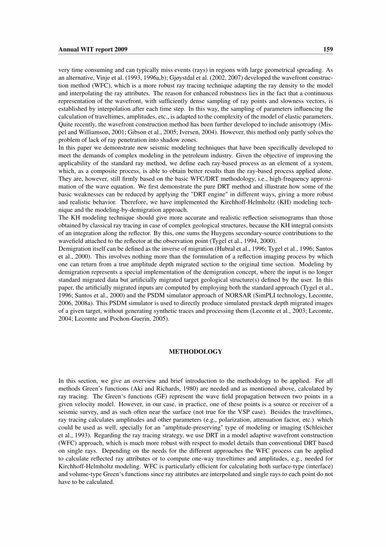
The second example contains three horizons, see Figure 8. The first reflector is a simple horizontal plane,the second a syncline structure as in the previous example and the deepest represents a (slightly smoothed)fault structure. For computational simplicity, we chose a 2.5D situation which means that 3D amplitudeeffects of in-plane propagation are correctly considered. In most ray-tracing applications for such a het-erogeneous subsurface, model smoothing is a key problem, and it is not always an easy task to determinethe proper smoothing procedure. Consequently, we would need a smooth version of the given model toproduce proper GF‘s for KH modeling and modeling by demigration which is in practice usual available asit is needed for migration anyway. Nevertheless, the obtained modeling result would be slightly differentdepending on the smoothing level and thus, would make a comparison with the DRT results more difficult.Therefore, we separate our layers by varying the densities and keep the velocities constant (vP = 2.0km/sand vS = 1.0km/s). The density is given by ρ1 = 1.0 g/cm3, ρ2 = 1.5 g/cm3, ρ3 = 2.0 g/cm3 and ρ4 = 2.5g/cm3, respectively.Gjøystdal et al. (2007) demonstrated that sharp edges on an interface can be smoothed slightly to producea diffraction-like DRT response, which is closer to reality than if keeping them sharp. Therefore, we em-ployed a smoothing operator to the fault interface, to obtain the best possible DRT synthetic seismogramfor this example.

168 Annual WIT report 2009

0

0

5

10

Depth[km]

X[km]

Figure 8: Second model consists of four layer, separated e.g, by a simple horizontal plane, a synclinestructure as in the previous example and a slightly smoothed fault structure.

As demonstrated for the first example, both demigration results show strong similarities, thus here werestrict ourselfs to the new SimPLI demigration approach. Again we consider a zero-offset survey alonga line in the x direction, with shot/receiver spacing of 50m and the shot/receivers being located between1 and 9km. The synthetic section resulting from modeling by demigration has been compared in Figure9 to the corresponding sections obtained by conventional seismic modeling schemes. Figure 9a showsthe modeled traces computed by standard ray tracing; Figure 9b contains the corresponding seismogramresulting from KH modeling with integral (2) and Figure 9c shows the new SimPLI demigration result.As expected, we observe differences between the standard ray tracing results and the ones obtained byboth summation processes. As in the previous example, the diffracted events, i.e., the caustic tails in thetriplication , are not present in the former. In this respect, the modeling by demigration approach is moreaccurate than the standard ray tracing because it includes diffracted-wave contributions as does the KHmodeling. However, there are no significant differences between the KH seismogram and the one obtainedby SimPLI demigration. To suppress the residual noise in the modeling by demigration result, we applied ahigh-frequency filter after the actual modeling process. However, the Simpli demigration yields practicallythe same pulse as standard ray tracing and KH modeling.

CONCLUSIONS

A major challenge in the development of ray-tracing technology is to achieve more robust applications ofthe ray method at the various stages of the seismic value chain - from acquisition to time lapse interpreta-tion. In this respect, one may either select a strategy based on specifically extending the validity area of thestandard ray method itself, or one may follow the red line of this paper, which is to consider ray tracing asonly one constituent of a composite system of processes.The combination of the standard ray method with the wavefront construction method serves a variety ofpurposes, e.g., simulation of large realistic 3D surveys and modeling the reflected wavefield for predefinedtargets and wave modes, as well as efficient generation of Green‘s function attributes needed for real dataimaging, simulated local imaging, and Kirchhoff modeling. The last technique turns out to be a very in-teresting candidate for effectively extending the limits of ray theory, since it dramatically reduces the needfor reflector smoothness, thereby modeling both edge and caustic diffractions. Although more time con-suming, it is quite feasible to perform Kirchhoff modeling in three dimensions today, having an efficientwavefront construction tracer running in parallel, even on small clusters.

ACKNOWLEDGMENTS

Special thanks to NORSAR Innovation AS for allowing us to use their seismic modelling software, and tothe Research Council of Norway (project # 181688/I30), for financial support. M.T. acknowledges supportby VISTA (Research Council of Norway) , via the ROSE project and the National Council of Scientific andTechnological Development (CNPq), Brazil. Additional support form the sponsors of the Wave InversionTechnology (WIT) Consortium is also acknowledged.

Annual WIT report 2009 169

b)

0

2

4

Tim

e [s]

2 4 6 8X[km]

a)

0

2

4

Tim

e [s]

2 4 6 8X[km]

c)

0

2

4

Tim

e [s]

2 4 6 8X[km]

Figure 9: Computed synthetic seismograms for different modeling techniques: (a) Kirchhoff Helmholtzmodeling, (b) standard ray-tracing and (c) SimPLI demigration.

170 Annual WIT report 2009

REFERENCES

Aki, K. and Richards, P. G. (1980). Quantitative seismology: Theory and Methods, Volume I. Freeman.

Cervený, V. (2001). Seismic Ray Theory. Cambridge University Press.

Eaton, D. W. and Clarke, G. (2000). A Kirchhoff integral method to model 3-D elastic wave scattering.70th Ann. Internat. Mtg., Soc. of Expl. Geophys., Expanded Abstracts, pages 2472–2475.

Frazer, L. N. and Sen, M. K. (1985). Kirchhoff-Helmholtz reflection seismograms in a laterally inhomo-geneous multi-layered elastic medium- I. Theory. Geophys. J. Roy. Astr. Soc., 80:121–147.

Gibson, R. L., Durussel, V., and Lee, K.-J. (2005). Modeling and velocity analysis with a wavefront-construction algorithm for anisotropic media. Geophysics, 70:T63–T74.

Gjøystdal, H., Iversen, E., Laurain, R., Lecomte, I., Vinje, V., and Åstebøl, K. (2002). Review of ray theoryapplications in modelling and imaging of seismic data. Studia geophysica et geodetica, 46:113–164.

Gjøystdal, H., Iversen, E., Lecomte, I., Kaschwich, T., Drottning, Å., and Mispel, J. (2007). Improvedapplicability of ray tracing in seismic acquisition, imaging, and interpretation. Geophysics, 72:SM261–SM271.

Hubral, P., Schleicher, J., and Tygel, M. (1996). A unified approach to 3-D seismic reflection imaging-PartI: Basic concepts. Geophysics, 61:742–758.

Iversen, E. (2004). Reformulated kinematic and dynamic ray tracing systems for arbitrarily anisotropicmedia. Studia geophysica et geodetica, 48:1–20.

Lecomte, I. (2004). Simulating Prestack Depth Migrated Sections. 66th Mtg. Eur. Assn. of Expl. Geophys.,Expanded Abstracts, P071.

Lecomte, I. (2006). Fremgangsmåte for simulering av locale prestakk dypmigrerte seismiske bilder. Nor-way patent #322089.

Lecomte, I. (2008a). Method simulating local prestack depth migrated seismic images. US patent#7,376,539.

Lecomte, I. (2008b). Resolution and illumination analyses in PSDM: A ray-based approach. The LeadingEdge, 27(5):650–663.

Lecomte, I. and Gelius, L. J. (1998). Have a look at the resolution of prestack depth migration for anymodel, survey and wavefields. 68th Ann. Internat. Mtg., Soc. of Expl. Geophys., Expanded Abstracts,SP 2.3.

Lecomte, I., Gjøystdal, H., and Drottning, Å. (2003). Simulated Prestack Local Imaging: a robust andefficient interpretation tool to control illumination, resolution, and timelapse properties of reservoirs.73th Ann. Internat. Mtg., Soc. of Expl. Geophys., Expanded Abstracts, pages 1525–1528.

Lecomte, I. and Pochon-Guerin, L. (2005). Simulated 2D/3D PSDM images with a fast, robust, and flexibleFFT-based filtering approach. 75th Ann. Internat. Mtg., Soc. of Expl. Geophys., Expanded Abstracts,pages 1810–1813.

Mispel, J. and Williamson, P. (2001). 3D Wavefront Construction for P and SV Waves in TransverselyIsotropic Media. 63th Mtg. Eur. Assn. of Expl. Geophys., Expanded Abstracts, page Session P094.

Santos, L. T., Schleicher, J., Hubral, P., and Tygel, M. (2000). Seismic modeling by demigration. Geo-physics, 65(4):1281–1289.

Schleicher, J., Tygel, M., and Hubral, P. (1993). 3-D true-amplitude finite-offset migration. Geophysics,58(8):1112–1126.

Annual WIT report 2009 171

Schleicher, J., Tygel, M., Ursin, B., and Bleistein, N. (2001). The Kirchhoff-Helmholtz integral foranisotropic, elastic media. Wave Motion, 34:353–364.

Spencer, C. P., Chapman, C. H., and Kragh, J. E. (1997). A fast, accurate integration method for Kirchhoff,Born and Maslov synthetic seismogram generation. 67th Ann. Internat. Mtg., Soc. of Expl. Geophys.,Expanded Abstracts, pages 1838–1841.

Toxopeus, G., Thorbecke, J., Wapenaar, K., Petersen, S., Slob, E., and J., F. (2008). Simulating migratedand inverted seismic data by filtering a geologic model. Geophysics, 73:T1–T10.

Tygel, M., Schleicher, J., and Hubral, P. (1994). Kirchhoff-Helmholtz theory in modelling and migration.J. Seis. Expl., 2:203–214.

Tygel, M., Schleicher, J., and Hubral, P. (1996). A unified approach to 3-D seismic reflection imaging- PartII: Theory. Geophysics, 61:759–775.

Tygel, M., Schleicher, J., Santos, L. T., and Hubral, P. (2000). An asymptotic inverse to the Kirchhoff-Helmholtz integral. Inverse Problems, 16:425–445.

Vinje, V., Iversen, E., Åstebøl, K., and Gjøystdal, H. (1996a). Estimation of multivalued arrivals in 3Dmodels using wavefront construction- Part I. Geophys. Prosp., 44:819–842.

Vinje, V., Iversen, E., Åstebøl, K., and Gjøystdal, H. (1996b). Part II: Tracing and interpolation. Geophys.Prosp., 44:843–858.

Vinje, V., Iversen, E., and Gjøystdal, H. (1993). Traveltime and amplitude estimation using wavefrontconstruction. Geophysics, 58:1157–1166.