RESEARCH PAPER

Synthetic seismograms for finite sources in spherically symmetricEarth using normal-mode summation

Tianshi Liu . Haiming Zhang

Received: 14 February 2017 / Accepted: 19 June 2017 / Published online: 28 August 2017

� The Author(s) 2017. This article is an open access publication

Abstract Normal-mode summation is the most rapidly

used method in calculating synthetic seismograms. How-

ever, normal-mode summation is mostly applied to point

sources. For earthquakes triggered by faults extending for

as long as several 100 km, the seismic waves are usually

simulated by point source summation. In this paper, we

attempt to follow a different route, i.e., directly calculate

the excitation of each mode, and use normal-mode sum-

mation to obtain the seismogram. Furthermore, we assume

the finite source to be a ‘‘line source’’ and numerically

calculate the transverse component of synthetic seismo-

grams for vertical strike-slip faults. Finally, we analyze the

features in the Love waves excited by finite faults.

Keywords Normal-mode summation � Syntheticseismogram � Finite fault � Surface waves

1 Introduction

The calculation of synthetic seismograms is one of the

most important topics in seismology, because on the one

hand, synthetic seismogram is the bridge that connects the

theory of seismology and the observational data, and on the

other hand, it is crucial to structure inversion and rupture

process inversion. Roughly speaking there are three types

of methods to calculate synthetic seismograms. The first

type is numerical method, e.g., the finite difference method

(Boore 1972), the finite element method (Bielak et al.

2003) and the spectral element method (Komatitsch and

Tromp 1999, 2002). Numerical methods are usually quite

flexible. They are available for very complex structures.

But the computational costs are usually high, and the

compromise between accuracy and efficiency is often

inevitable. The second type is asymptotic method, e.g., the

generalized ray method (Gilbert and Helmberger 1972) and

the WKBJ method (Chapman 1978). The asymptotic

methods typically have high efficiency, but only effective

for computing the high-frequency component. The third

type is semi-analytical method, e.g., the discrete

wavenumber method (Bouchon and Aki 1977) and the R/T

coefficient method (Luco and Apsel 1983; Kennett and

Kerry 1979) for stratified half-space, and the normal-mode

summation method (Dahlen and Tromp 1998) for spheri-

cally symmetric Earth model.

Normal-mode summation is one of the most widely used

methods in simulating teleseismic waves. After the 1960

Chile earthquake, seismologists did a great amount of

studies on normal modes and gradually developed the

normal-mode summation method. Gilbert (1971) explicitly

showed the normal-mode summation representation of the

displacement in elastic media. Singh and Ben-Menahem

(1969a, b) calculated the excitation of each mode by a

point source in spherically symmetric Earth. Takeuchi and

Saito (1972) derived the equations that govern the normal

modes. Tanimoto (1984) obtained the formulae to calculate

long-period synthetic seismograms using normal-mode

summation. Woodhouse (1988) developed the numerical

method to calculate the radial eigenfunction, which made it

possible to calculate synthetic seismograms using normal-

mode summation. Dahlen and Tromp (1998) integrated the

previous work and constructed a comprehensive and

T. Liu � H. Zhang (&)

Department of Geophysics, School of Earth and Space Sciences,

Peking University, Beijing 100871, People’s Republic of China

e-mail: zhanghm@pku.edu.cn

T. Liu

e-mail: dash2007@163.com

123

Earthq Sci (2017) 30(3):125–133

DOI 10.1007/s11589-017-0188-1

compact framework for theoretical global seismology,

which includes the normal-mode theory, normal-mode

summation method and other related topics.

However, normal-mode summation is mostly used for

point sources. In order to calculate the synthetic seismo-

gram for a finite source, point source summation is usually

used (Bouchon 1980a, b; Song and Helmberger 1996): the

fault is discretized into small sub-faults which can be

treated as point sources; the seismogram for each sub-fault

is calculated using normal-mode summation and then the

seismogram for the finite fault is obtained by adding the

seismograms of the sub-faults together. Analytical or semi-

analytical methods are sometimes applied to calculating the

synthetic seismograms of finite faults (Ben-Menahem and

Singh 1987; Israel and Kovach 1977; Saikia and Helm-

berger 1997; Stump and Johnson 1982).

In this work, we expand the normal-mode summation

method to the finite fault case. We first derive the excita-

tion of each mode and then add them together to obtain the

seismogram. We assume that the fault is a ‘‘line source’’: it

expand transversely but concentrate at a certain depth

radially, which take into account the effect of propagation

in the transverse direction, but ignore that of the propa-

gation in the radial direction. We represent the normal

mode in the form of generalized spherical harmonics

(Phinney and Burridge 1973; Yang et al. 2010). Next, we

use the radial eigenfunction of MINEOS (Woodhouse

1988) and calculate the numerically results of the trans-

verse component in the case of the vertical strike-slip fault

as example. We then observe some features in the Love

wave of the finite source, and we use an intuitive model to

explain these features based on Chap.10 of Aki and

Richards (2002).

2 Normal-mode summation for finite source

2.1 From point source to finite source

Suppose that the displacement at x excited by a point

source at x0 can be written in the form of normal-mode

summation as

gðx; t; x0Þ ¼X

k

Akðx0; tÞskðxÞ; ð1Þ

in which sk is the eigenfunction with index k, and Ak

represents the excitation of mode with index k by the point

source at x0. Note that here the source does not have to be a

body force, so g is not necessarily the Green’s function. For

a finite source with a spatial and temporal amplitude

distribution Dðx0; sÞ, the displacement at x is

uðx; tÞ ¼Z

Rf

Z Tf

0

gðx; t � s; x0ÞDðx0; sÞdsdS

¼X

k

Z

Rf

Z Tf

0

Akðx0; t � sÞDðx0; sÞdsdS !

skðxÞ;

ð2Þ

where Rf is the fault plane, Tf is the total rupture time.

Thus, the seismogram of the finite fault can also be written

in the normal-mode summation form

uðx; tÞ ¼X

k

AkðtÞskðxÞ; ð3Þ

where the excitation of mode with index k is

AkðtÞ ¼Z

Rf

Z Tf

0

Akðx0; t � sÞDðx0; sÞdsdS: ð4Þ

The excitation of mode with index k by a double-couple M

is well known (Dahlen and Tromp 1998; Yang et al. 2010),

Akðx0; tÞ ¼ M : e�kðx0Þ� � 1� e�rkt cosxkt

x2k

: ð5Þ

Substitute Eq. (5) in Eq. (4), and let

_mðx0; sÞ ¼ MDðx0; sÞ; ð6Þ

we obtain

AkðtÞ ¼Z

Rf

Z Tf

0

_mðx0; sÞ : e�kðx0Þ� �

� 1� e�rkðt�sÞ cosxkðt � sÞx2

k

dsdS:

ð7Þ

2.2 GSH representation for spherically symmetric

Earth

Any tensor can be decomposed in generalized spherical

coordinate, and the components can be represented using

generalized spherical harmonics (GSH). We assume that

the Earth structure is spherically uniform, and we can write

the normal modes using GSH. Then, we use Eqs. (7) and

(2) to obtain the final solution of the displacement excited

by finite source.

The normal mode of the spherical symmetric Earth is

(Dahlen and Tromp 1998)

skðr; h;/Þ ¼X

a¼ 0;�1

sanlðrÞYalmðh;/Þea; ð8Þ

where Yalm is the generalized scalar harmonics, ea is the

base of generalized spherical coordinate. For a spheroidal

or a toroidal mode, the index k is the same as n, l, m.

126 Earthq Sci (2017) 30(3):125–133

123

s�1nl ¼ 1ffiffiffi

2p Vnl; s0nl ¼ Unl ð9Þ

for spheroidal mode, and

s�1nl ¼ � 1ffiffiffi

2p Wnl; s0nl ¼ 0 ð10Þ

for toroidal mode, where Unl, Vnl and Wnl are radial

eigenfunctions.

Substituting Eq. (8) into Eqs. (7) and (2), we can derive

the representation of seismogram using GSH. But before

this, we make some simplifications. First, without loss of

generality, we can put our spherical coordinate such that

the line connecting the pole and the origin is perpendicular

to the fault plane (see Fig. 1). In such coordinate, the

coordinate of the receiver is fr; h;/g, the coordinate of

some point on the fault plane is fr0; h0;ug. We set up a

local coordinate fn; /; mg on the fault plane. Using this

coordinate system,

dS ¼ r0 sin h0dndu: ð11Þ

Next, we assume that the fault only expands transversely,

but concentrates at a certain depth (line source). Unlike the

point source approximation, which concentrates the

seismic moment at a single point, the line source

approximation assumes that the seismic moment

concentrates on a line. It is a more general assumption

than the point source approximation, and it captures the

effect of the lateral propagation of the rupture, but it is still

far from enough to capture the full finite fault feature of the

earthquake. The line source approximation is valid because

the impact of the transverse propagation of rupture is far

more significant compared with the radial propagation.

Thus, the integral on the fault can be simplified as

dS ¼ rf w sin hddu; ð12Þ

where w is the width of the fault, hd is the dip-angle of thefault plane, and rf is the distance between the fault and the

origin.

Using the aforementioned spherical coordinate and the

line source approximation, we obtain the GSH represen-

tation of displacement triggered by the finite fault. We useKc u

q to represent the displacement in q direction

(q ¼ Z;R; T for each direction of the ZRT coordinate),

related to K type mode (K ¼ S; T for spheroidal and tor-

oidal mode) triggered by c component of slip (c ¼ u; n for

strike-slip and dip-slip component). For simplicity, we

show only the result of displacement that related to toroidal

mode and triggered by strike-slip component

Tuu

Znl ¼ 0;

Tuu

Rnl ¼

X

n;l

�2sinhdWnlðrÞTS2nlR ei/b

TuK

�2;þ1nl þ T

uKþ2;þ1nl

2

( )

þ coshdWnlðrÞTS1nlR ei/b

TuK

�1;þ1nl � T

uKþ1;þ1nl

2

( );

Tuu

Tnl ¼

X

n;l

�2sinhdWnlðrÞTS2nlI ei/b

TuK

�2;þ1nl þ T

uKþ2;þ1nl

2

( )

þ cos2hdWnlðrÞTS1nlI ei/b

TuK

�1;þ1nl � T

uKþ1;þ1nl

2

( );

ð13Þ

where TS1nl,

TS2nl and

Kc K

a;bnl are given in ‘‘Appendix.’’ /b

is the back-azimuth angle (see Fig. 1). Other parts of dis-

placement are shown in ‘‘Appendix.’’ Note that as the

length of the fault goes to zero, the formulae for the dis-

placements due to a finite source become exactly the same

as the point source case (Yang et al. 2010).

3 Numerical results

To show the impact of the transverse propagation of rup-

ture on seismograms, we continue to make following

simplifications:

(i) The fault is vertical and the slip only has strike-slip

component, i.e., hd ¼ p2,

(ii) The rupture velocity is a pulse propagating along the

fault with a constant velocity, which is

Fig. 1 Geometry of the receiver and the finite source. The global

spherical coordinate is selected such that the line connecting the

origin and the ‘‘Northpole’’ is perpendicular to the fault plane. The

local coordinate at the receiver (x) is the ‘‘ZRT’’ coordinate. The basis

of local coordinate at the receiver is fn; /; mg. The reference point of

the source is x0, which can be an arbitrary point near the fault (e.g.,

epicenter). The angular distance between the reference point and the

receiver is defined as the epicentral distance D. The back-azimuth is

/b

Earthq Sci (2017) 30(3):125–133 127

123

D _suðu; sÞ ¼ D _s0d s� uvf

� �; ð14Þ

where the rupture velocity vf is constant, and with unit

rad=s.

(iii) The receiver coplanar to the fault plane.

We calculate the synthetic seismograms in different

scenarios (different rupture length and rupture velocity,

rupture toward and away from the receiver, respectively),

show the features of seismograms of finite fault and

compare them with the seismograms of point source, which

is exactly the same as the result of MINEOS. Table 1

shows the source and structure parameters we use for our

numerical calculation. Note that the source parameters are

chose according to the study of the 1992 Landers

earthquake (Wald and Heaton 1994).

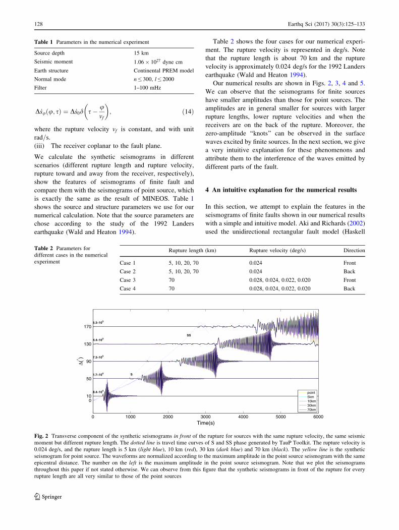
Table 2 shows the four cases for our numerical experi-

ment. The rupture velocity is represented in deg/s. Note

that the rupture length is about 70 km and the rupture

velocity is approximately 0.024 deg/s for the 1992 Landers

earthquake (Wald and Heaton 1994).

Our numerical results are shown in Figs. 2, 3, 4 and 5.

We can observe that the seismograms for finite sources

have smaller amplitudes than those for point sources. The

amplitudes are in general smaller for sources with larger

rupture lengths, lower rupture velocities and when the

receivers are on the back of the rupture. Moreover, the

zero-amplitude ‘‘knots’’ can be observed in the surface

waves excited by finite sources. In the next section, we give

a very intuitive explanation for these phenomenons and

attribute them to the interference of the waves emitted by

different parts of the fault.

4 An intuitive explanation for the numerical results

In this section, we attempt to explain the features in the

seismograms of finite faults shown in our numerical results

with a simple and intuitive model. Aki and Richards (2002)

used the unidirectional rectangular fault model (Haskell

Table 1 Parameters in the numerical experiment

Source depth 15 km

Seismic moment 1:06� 1027 dyne cm

Earth structure Continental PREM model

Normal mode n� 300, l� 2000

Filter 1–100 mHz

Table 2 Parameters for

different cases in the numerical

experiment

Rupture length (km) Rupture velocity (deg/s) Direction

Case 1 5, 10, 20, 70 0.024 Front

Case 2 5, 10, 20, 70 0.024 Back

Case 3 70 0.028, 0.024, 0.022, 0.020 Front

Case 4 70 0.028, 0.024, 0.022, 0.020 Back

0 1000 2000 3000 4000 5000 6000

010

50

90

130

170

Time(s)

Δ (° )

8.4×104

1.7×104

7.3×103

4.4×103

5.3×103

S

SS

point5km10km30km70km

Fig. 2 Transverse component of the synthetic seismograms in front of the rupture for sources with the same rupture velocity, the same seismic

moment but different rupture length. The dotted line is travel time curves of S and SS phase generated by TauP Toolkit. The rupture velocity is

0.024 deg/s, and the rupture length is 5 km (light blue), 10 km (red), 30 km (dark blue) and 70 km (black). The yellow line is the synthetic

seismogram for point source. The waveforms are normalized according to the maximum amplitude in the point source seismogram with the same

epicentral distance. The number on the left is the maximum amplitude in the point source seismogram. Note that we plot the seismograms

throughout this paper if not stated otherwise. We can observe from this figure that the synthetic seismograms in front of the rupture for every

rupture length are all very similar to those of the point sources

128 Earthq Sci (2017) 30(3):125–133

123

model) to explain the spectral features of the surface

waves. Using this idea, we can qualitatively explain the

variation of amplitudes of the Love waves due to the

rupture length and velocity of the finite faults in time

domain. Suppose that we have a 1-D plane dispersive wave

excited by a point source

f ðx; tÞ ¼ 1ffiffiffiffiffiffi2p

pZ þ1

�1FðxÞe

ix xvðxÞ�t

� �

dx; ð15Þ

in which FðxÞ denotes the spectrum, and vðxÞ is the phasevelocity. For the finite source case, the wave field can be

represented as the integral over the source

f ðx; tÞ ¼ 1ffiffiffiffiffiffi2p

pZ l

�l

Z þ1

�1

FðxÞ2l

eix x�x0

vðxÞ�ðt�t0ðx0ÞÞ� �

dxdx0;

ð16Þ

where t0 is the time that the rupture arrives at x0. If we

further assume that the rupture propagates at a constant

velocity vr, then Eq. (16) becomes

f ðx; tÞ ¼ 1ffiffiffiffiffiffi2p

pZ þ1

�1FðxÞcðxÞe

ix xvðxÞ�t

� �

dx; ð17Þ

where

0 1000 2000 3000 4000 5000 6000

010

50

90

130

170

Time(s)

Δ(° )

8.4×103

1.7×103

7.3×103

5.3×103

S

SS

4.4×103

point5km10km30km70km

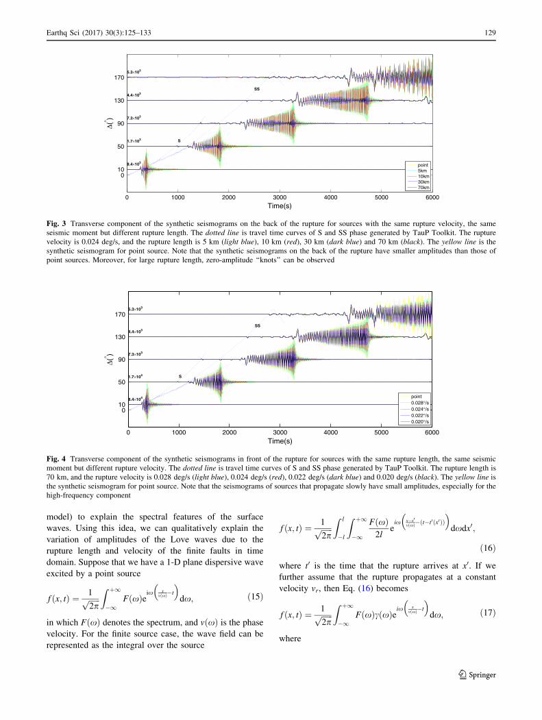
Fig. 3 Transverse component of the synthetic seismograms on the back of the rupture for sources with the same rupture velocity, the same

seismic moment but different rupture length. The dotted line is travel time curves of S and SS phase generated by TauP Toolkit. The rupture

velocity is 0.024 deg/s, and the rupture length is 5 km (light blue), 10 km (red), 30 km (dark blue) and 70 km (black). The yellow line is the

synthetic seismogram for point source. Note that the synthetic seismograms on the back of the rupture have smaller amplitudes than those of

point sources. Moreover, for large rupture length, zero-amplitude ‘‘knots’’ can be observed

0 1000 2000 3000 4000 5000 6000

010

50

90

130

170

Time(s)

Δ(° )

8.4×104

1.7×104

7.3×103

4.4×103

5.3×103

S

SS

point0.028°/s0.024°/s0.022°/s0.020°/s

Fig. 4 Transverse component of the synthetic seismograms in front of the rupture for sources with the same rupture length, the same seismic

moment but different rupture velocity. The dotted line is travel time curves of S and SS phase generated by TauP Toolkit. The rupture length is

70 km, and the rupture velocity is 0.028 deg/s (light blue), 0.024 deg/s (red), 0.022 deg/s (dark blue) and 0.020 deg/s (black). The yellow line is

the synthetic seismogram for point source. Note that the seismograms of sources that propagate slowly have small amplitudes, especially for the

high-frequency component

Earthq Sci (2017) 30(3):125–133 129

123

cðxÞ ¼ sinc xl1

vr� 1

vðxÞ

� � ¼ sinc½pðnt � nlÞ�: ð18Þ

nt and nl are ratios of rupture time over period of wave and

rupture length over wavelength,

nt ¼Tr

T; nl ¼

2l

k: ð19Þ

Here we define vr and Tr to be negative if the rupture

propagates away from the receiver. The ‘‘sinc’’ function in

Eq. (17) is

sincðxÞ ¼ sin x

x; ð20Þ

the graph of which is shown in Fig. 6.

Note that the only difference between the wave field

excited by point source Eq. (15) and that by finite source

Eq. (17) is the existence of c, which is the amplification

coefficient due to the effect of finite source. Then, we can

discuss the amplitude of wave in frequency domain.

Table 3 shows the value of nt � nl in different scenarios.

The dispersion relation for PREM model is given by Wid-

mer-Schnidrig and Laske (2009). According to our model, if

jnt � nlj 0 then c 1, the wave emitted by all parts of the

source arrives approximately at the same time, the amplitude

is almost as large in the wave field produced by finite source

as by point source; if jnt � nlj 1, then c 0, which

means that the amplitude is greatly diminished due to the

destructive interference of the wave emitted by different

parts of the source. The idea here is essentially the same as

in Vallee and Dunham (2012). Moreover, if nt � nl is a

nonzero integer, c ¼ 0 which indicates the position of the

zero-amplitude ‘‘knot.’’ From Table 3, we can see that

(i) For the same rupture length and velocity, the finiteness

of the fault impacts more on high-frequency compo-

nent than on low-frequency component;

(ii) For the same frequency, the waves produced by

longer faults have smaller amplitudes than those

produced by shorter faults;

(iii) The waves have larger amplitude in front of the

rupture than in the back and have more zero-

amplitude knots,

which correspond exactly to what we observe in the

numerical results. Moreover, note in Table 3 that when

rupture length 111.2 km, rupture velocity 0.020 deg/s

and frequency f ¼ 50 mHz, the nt � nl value is very

close to 1, which predicts the zero-amplitude knot.

Actually, we can observe the knot in the synthetic

seismogram exactly correspond to the 50 mHz group

velocity (Fig. 7).

0 1000 2000 3000 4000 5000 6000

010

50

90

130

170

Time(s)

Δ(° )

8.4×104

1.7×104

7.3×103

4.4×103

5.3×103

S

SS

point0.028°/s0.024°/s0.022°/s0.020°/s

Fig. 5 Transverse component of the synthetic seismograms in front of the rupture for sources with the same rupture length, the same seismic

moment but different rupture velocity. The dotted line is travel time curves of S and SS phase generated by TauP Toolkit. The rupture length is

70 km, and the rupture velocity is 0.028 deg/s (light blue), 0.024 deg/s (red), 0.022 deg/s (dark blue) and 0.020 deg/s (black). The yellow line is

the synthetic seismogram for point source. Note that the synthetic seismograms on the back of the rupture have smaller amplitudes than those of

point sources. Moreover, for large rupture length, zero-amplitude ‘‘knots’’ can be observed

Fig. 6 Graph of the ‘‘sinc’’ function. sincð0Þ ¼ 1 is the maximum of

the function, and the value rapidly decays away from 0. Moreover,

sincðnpÞ ¼ 0 for n is nonzero integer

130 Earthq Sci (2017) 30(3):125–133

123

5 Conclusion

In this paper, we expand the normal-mode method to the

finite source case. Instead of using point source summa-

tion, we directly calculate the excitation of each mode by

the finite fault and add together to obtain the synthetic

seismogram. We derive the solution of displacement

produced by a ‘‘line source’’ and carry out numerical

experiments and discuss the impact of rupture length and

rupture velocity on the wave form of synthetic seismo-

gram, especially the wave form of Love wave. We

observe that

(i) The amplitude is smaller in the seismogram of finite

fault than that of point source with the same seismic

moment;

(ii) The finiteness of fault has more significant impact on

high-frequency component than on low-frequency

component;

(iii) The amplitude in the seismogram of finite fault is

diminished more for the receiver that in the back of

the rupture;

(iv) Zero-amplitude ‘‘knots’’ exist, and there are more

‘‘knots’’ in the back of the rupture.

Moreover, we use the Haskell model and the interference

of waves emitted by different parts of the fault to provide a

very intuitive explanations for all these phenomenons.

Although this model is too simple to explain all the features

in different cases accurately and qualitatively, it describes

the basic characters of the seismogram of finite faults.

However, there are still some problems remain to be dealt

with. The first one is the inclusion of radial propagation of

the rupture. In this paper, we treat the fault as the ‘‘line

source,’’ which is far from enough. The line source model

can only capture the effect of rupture propagation in the

transverse direction. Although this is a step forward com-

pared with the point source model, it still cannot take into

account all the features on the fault. The second one is the

efficiency of the method. The finiteness of the source causes

the unavailability of the additional theorem of GSH, which

means that the summation over m needs to be numerically

calculated. Such summation is quite inefficient numerically.

These two problems must be solved in order for this method

to be usable in the calculation of synthetic seismograms.

Acknowledgements This work was supported by the National Nat-

ural Science Foundation of China (Grant No. 41674050) and MOST

grant (2012CB417301). We thank the two anonymous reviewers for

Table 3 Values of nt � nl for

some combinations of rupture

length, rupture velocity and

frequency

Rupture length (km) Rupture velocity (s/deg) 3 mHz 10 mHz 20 mHz 50 mHz 100 mHz

70 0.024 0.0276 0.0744 0.1199 0.2120 0.2662

70 0.020 0.0540 0.1626 0.2962 0.6527 1.1475

111.2 0.020 0.0858 0.2583 0.4705 1.0368 1.8229

10 0.020 0.0077 0.0232 0.0423 0.0932 0.1639

70 -0.024 -0.1084 -0.3788 -0.7866 -2.0541 -4.2662

70 -0.020 -0.1348 -0.4669 -0.9628 -2.4948 -5.1475

0 1000 2000 3000 4000 5000 6000

010

50

90

130

170

Time(s)

Δ(° )

1.6×103

3.3×102

1.6×102

1.3×102

1.8×103

50mHz 100mHz

10mHz

20mHz

Fig. 7 Zero-amplitude ‘‘knots’’ in synthetic seismograms. Note that they exist near the position that correspond to the group velocity of 50 mHz

Love wave

Earthq Sci (2017) 30(3):125–133 131

123

their constructive comments and suggestions which are crucial to the

improvement of our manuscript.

Open Access This article is distributed under the terms of the

Creative Commons Attribution 4.0 International License (http://crea

tivecommons.org/licenses/by/4.0/), which permits unrestricted use,

distribution, and reproduction in any medium, provided you give

appropriate credit to the original author(s) and the source, provide a

link to the Creative Commons license, and indicate if changes were

made.

Appendix: Formulae for the synthetic seismograms

of finite faults

The displacement triggered by the finite fault is

Snu

Z ¼X

n;l

sin 2hdUnlðrÞ SS0nlSnK

0;0nl � SS2

nlRSnK

�2;0nl

n o� �

cos 2hdUnlðrÞSS2nlR

SnK

�1;0nl

n o;

Snu

R ¼X

n;l

sin 2hdVnlðrÞ SS0nlR ei/b S

nK0;þ1nl

n o�

� SS2nlR ei/b

SnK

�2;þ1nl þ S

nKþ2;þ1nl

2

( )!

þ cos 2hdVnlðrÞSS1nlR ei/b

SnK

�1;þ1nl � S

nKþ1;þ1nl

2

( );

Snu

T ¼X

n;l

� sin 2hdVnlðrÞ SS0nlI ei/b S

nK0;þ1nl

n o�

� SS2nlI ei/b

SnK

�2;þ1nl þ S

nKþ2;þ1nl

2

( )!

� cos 2hdVnlðrÞSS1nlI ei/b

SnK

�1;þ1nl � S

nKþ1;þ1nl

2

( );

ð21ÞTnu

Z ¼ 0;

Tnu

R ¼X

n;l

sin2hdWnlðrÞTS2nlR ei/b

TnK

�2;þ1nl � T

nKþ2;þ1nl

2

( )

� cos2hdWnlðrÞTS1nlR ei/b

TnK

�1;þ1nl þ T

nKþ1;þ1nl

2

( );

Tnu

T ¼X

n;l

�sin2hdWnlðrÞTS2nlI ei/b

TnK

�2;þ1nl � T

nKþ2;þ1nl

2

( )

þ cos2hdWnlðrÞTS1nlI ei/b

TnK

�1;þ1nl þ T

nKþ1;þ1nl

2

( );

ð22Þ

Suu

Z ¼X

n;l

2sinhdUnlðrÞSS2nlI

SuK

�2;0nl

n o

� coshdUnlðrRÞSS2nlI

SnK

�1;0nl

n o;

Suu

R ¼X

n;l

2sinhdVnlðrÞSS2nlI ei/b

SuK

�2;þ1nl � S

uKþ2;þ1nl

2

( )

� coshdVnlðrÞSS1nlI ei/b

SuK

�1;þ1nl þ S

uKþ1;þ1nl

2

( );

Suu

R ¼X

n;l

2sinhdVnlðrÞSS2nlR ei/b

SuK

�2;þ1nl � S

uKþ2;þ1nl

2

( )

� coshdVnlðrÞSS1nlR ei/b

SuK

�1;þ1nl þ S

uKþ1;þ1nl

2

( );

ð23ÞTuu

Z ¼ 0;

Tuu

R ¼X

n;l

�2sinhdWnlðrÞTS2nlR ei/b

TuK

�2;þ1nl þ T

uKþ2;þ1nl

2

( )

þ coshdWnlðrÞTS1nlR ei/b

TuK

�1;þ1nl � T

uKþ1;þ1nl

2

( );

Tuu

T ¼X

n;l

�2sinhdWnlðrÞTS2nlI ei/b

TuK

�2;þ1nl þ T

uKþ2;þ1nl

2

( )

þ cos2hdWnlðrÞTS1nlI ei/b

TuK

�1;þ1nl � T

uKþ1;þ1nl

2

( );

ð24Þ

where

SS0nl ¼ _Unlðrf Þ þ

1

rf

ffiffiffiffiffiffiffiffiffiffiffiffiffiffiffilðlþ 1Þ

p

2Vnlðrf Þ � Unlðrf Þ

!;

SS1nl ¼ _Vnlðrf Þ þ

1

rf

ffiffiffiffiffiffiffiffiffiffiffiffiffiffiffilðlþ 1Þ

pUnlðrf Þ � Vnlðrf Þ

� �;

SS2nl ¼

ffiffiffiffiffiffiffiffiffiffiffiffiffiffiffiffiffiffiffiffiffiffiffiffiffiffiffiðl� 1Þðlþ 2Þ

p

2rfVnlðrf Þ;

ð25Þ

TS1nl ¼ _Wnlðrf Þ�

Wnlðrf Þrf

; TS2nl ¼

ffiffiffiffiffiffiffiffiffiffiffiffiffiffiffiffiffiffiffiffiffiffiffiffiffiðl�1Þðlþ2Þ

p

2rfWnlðrf Þ;

ð26Þ

and

132 Earthq Sci (2017) 30(3):125–133

123

Kc K

a;bnl ðx; tÞ¼

2lþ1

4plwrf sinhd

�Xþl

m¼�l

PalmðcoshdÞP

blmðcoshÞeim/

Z u2

u1

Z Tf

0

D _scðu;sÞe�imu

�1�e�Krnlðt�sÞ cosKxnlðt� sÞ

Kx2nl

dsdu

!:

ð27Þ

References

Aki K, Richards PG (2002) Quantitative seismology, 2nd edn.

University Science Books, Sausalito, pp 491–536

Ben-Menahem A, Singh SJ (1987) Supershear accelerations and

Mach-waves from a rupturing front-I. Theoretical model and

implications. J Phys Earth 35:347–365

Bielak J, Loukakis K, Hisada Y, Yoshimura C (2003) Domain

reduction method for three-dimensional earthquake modeling in

localized regions, part I: theory. Bull Seismol Soc Am

93:817–824

Boore DM (1972) Finite-difference methods for seismic wave

propagation in heterogeneous materials. In: Bolt BA (ed)

Methods in computational physics. Academic Press, NY,

pp 1–37

Bouchon M, Aki K (1977) Discrete wave-number representation of

seismic-source wave fields. Bull Seismol Soc Am 67:259–277

Bouchon M (1980a) The motion of the ground during and earthquake

1. The case of a strike slip fault. J Geophys Res 85:356–366

Bouchon M (1980b) The motion of the ground during and earthquake

2. The case of a dip slip fault. J Geophys Res 85:367–375

Chapman CH (1978) A new method for computing synthetic

seismograms. Geophys J R Astron Soc 54:481–518

Dahlen FA, Tromp J (1998) Theoretical global seismology. Princeton

University Press, Princeton, pp 363–404

Gilbert F (1971) Excitation of normal modes of earth by earthquake

sources. Geophys J R Astron Soc 22:223–226

Gilbert F, Helmberger DV (1972) Generalized ray theory for a

layered sphere. Geophys J R Astron Soc 27:57–80

Israel M, Kovach RL (1977) Near-field motions from a propagating

strike-slip fault in an elastic Half-space. Bull Seismol Soc Am

67:977–994

Kennett BLN, Kerry NJ (1979) Seismic wave in a stratified half

space. Geophys J Int 57:557–583

Komatitsch D, Tromp J (1999) Introduction to the spectral element

method for three-dimensional seismic wave propagation. Geo-

phys J Int 139:806–822

Komatitsch D, Tromp J (2002) Spectral-element simulations of global

seismic wave propagation-II. Three-dimensional models, oceans,

rotation and self-gravitation. Geophys J Int 150:303–318

Luco JE, Apsel RJ (1983) On the Green’s functions for a layered half-

space. Part I. Bull Seismol Soc Am 73:909–929

Phinney RA, Burridge R (1973) Representation of elastic-gravita-

tional excitation of a spherical earth model by generalized

spherical harmonics. Geophys J R Astron Soc 34:451–487

Saikia CK, Helmberger DV (1997) Approximation of rupture

directivity in regional phases using upgoing and downgoing

wave fields. Bull Seismol Soc Am 87:987–998

Singh SJ, Ben-Menahem A (1969a) Eigenvibrations of the earth

excited by finite dislocations-I. Toroidal oscillations. Geophys J

R Astron Soc 17:151–177

Singh SJ, Ben-Menahem A (1969b) Eigenvibrations of the earth

excited by finite dislocations-II. Spheroidal oscillations. Geo-

phys J R Astron Soc 17:333–350

Song XJ, Helmberger DV (1996) Source estimation of finite faults

from broadband regional networks. Bull Seismol Soc Am

86:797–804

Stump BW, Johnson LR (1982) Higher-degree moment tensors-the

importance of source finiteness and rupture propagation on

seismograms. Geophys J R Astron Soc 69:721–743

Takeuchi H, Saito M (1972) Seismic surface waves. In: Bruce AB

(ed) Seismology: surface waves and earth oscillations, volume

11 of methods in computational physics. Academic Press, New

York, pp 217–295

Tanimoto T (1984) A simple derivation of the formula to calculate

synthetic long-period seismograms in a heterogeneous earth by

normal mode summation. Geophys J R Astron Soc 77:275–278

Vallee M, Dunham EM (2012) Observation of far-field Mach waves

generated by the 2001 Kokoxili supershear earthquake. Geophys

Res Lett 39:L05311

Wald DJ, Heaton TH (1994) Spatial and temporal distribution of slip

for the 1992 Landers, California, earthquake. Bull Seismol Soc

Am 84:668–691

Widmer-Schnidrig R, Laske G (2009) Theory and observations-

normal modes and surface wave measurements. In: Dziewonski

AM, Romanowicz BZ (eds) Seismology and structure of the

earth: treatise on geophysics. Elsevier, Amsterdam, pp 67–125

Woodhouse JH (1988) The calculation of the eigenfrequencies and

eigenfunctions of the free oscillations of the Earth and the Sun.

In: Doorbos DJ (ed) Seismological algorithms. Academic Press,

San Diago, pp 321–370

Yang H-Y, Zhao L, Hung S-H (2010) Synthetic seismograms by

normal-mode summation: a new derivation and numerical

examples. Geophys J Int 183:1613–1632

Earthq Sci (2017) 30(3):125–133 133

123