P - 133

Migration Velocity Analysis for Tilted TI media: Application to Synthetic Data

Laxmidhar Behera*, National Geophysical Research Institute, India and Center for Wave Phenomena, Colorado School of Mines, USA; and

Ilya Tsvankin, Center for Wave Phenomena, Colorado School of Mines, USA

Summary

Tilted transversely isotropic (TTI) formations cause severe imaging problems in active tectonic areas (e.g., fold-and thrust-belts) and in subsalt exploration plays. Here, we introduce a methodology for P-wave prestack depth imaging in TTI media that properly accounts for the tilt of the symmetry axis as well as for spatial velocity variations. For purposes of migration velocity analysis (MVA), the model is divided into blocks with constant values of the anisotropy parameters �and �having linearly varying symmetry-direction velocity VP0 controlled by the vertical (kz) and lateral (kx) gradients. Since tilt is not well constrained by P-wave data, the symmetry axis is kept orthogonal to the reflectors in all trial velocity models. The MVA algorithm estimates the velocity gradients kz and kx and the anisotropy parameters �and �in the layer-stripping mode. We have also performed synthetic tests on different models like syncline, thrust-sheet etc., having tilted layers to confirm the robustness of our MVA algorithm. This shows that by ignoring the influence of tilt may lead to significant image distortions and errors in the parameter estimation. The ability of our MVA algorithm to separate the anisotropy parameters from velocity gradients can also be used in lithology discrimination and geologic interpretation of seismic data in complex areas.

Introduction

Transverse isotropy with tilted symmetry axis (TTI) describes dipping shale layers in fold-and-thrust belts and near salt bodies (e.g., Tsvankin, 2005). TTI symmetry can also be caused by a system of parallel dipping fractures embedded in otherwise isotropic rock (Dewangan and Tsvankin, 2006a). Serious distortions in image quality are caused by TTI layers with conventional (isotropic) seismic imaging are well documented in the literature (e.g., Vestrum et al., 1999; Kumar et al., 2004). Since the influence of tilt creates ambiguity in parameter estimation, a major problem in seismic processing for TTI media is accurate velocity analysis and model building.

P-wave kinematic signatures for tilted transverse isotropy can be described by the symmetry-direction velocity VP0, Thomsen parameters �and �, and the orientation of the symmetry axis. In 2D models treated here, the symmetry direction is described by the angle

�(tilt) with the vertical. Estimation of this parameter set even for a single TTI layer generally requires combining P-wave data with mode converted PS-waves (Dewangan and Tsvankin, 2006a, 2006b). For shale layers, however the symmetry axis is usually orthogonal to the layer boundaries, which helps to make velocity analysis more stable.

Here, we present an extension of MVA algorithmdeveloped for VTI media by Sarkar and Tsvankin (2004, 2006) to tilted transverse isotropy. The symmetry axis is assumed to be orthogonal to the reflectors and confined to the vertical incidence plane. The model is composed of “quasi-factorized” TTI blocks, in which the Thomsen parameters �and �are constant, while the symmetry direction velocity VP0 is a linear function of the spatial coordinates. These blocks are not strictly factorized because reflectors may have arbitrary shape, and the symmetry axis orientation may vary within each block. The velocity analysis and imaging results are compared with those

obtained by VTI algorithms to illustrate the need to account for tilt in anisotropic imaging.

Methodology

For TI layers with the symmetry axis orthogonal to the reflector, the dip-line P-wave normal-moveout (NMO) velocity is described by the isotropic cosine-of-dip dependence (Tsvankin, 2005):

is the ray parameter of the zero-offset ray;note that p can be determined from the time slopes on the zero-offset or stacked section. In some cases (e.g., for a bending layer), it may be possible to directly estimate the zero-dip NMO velocity given by

Then equation 1 can be used to find the vertical velocity VP0, which can be substituted into equation 2 to obtain �. In our algorithm, the velocity VP0 is assumed to be known at the top of each block, so �can be determined directly from the NMO velocity in equation 1. The parameter �is not constrained by NMO velocity and has to be estimated fromnonhyperbolic moveout controlled by the anellipticityparameter _ �(�−�)/(1 2�) (Pech et al., 2003). To make the modeling and migration algorithms of Sarkarand Tsvankin (2004) suitable for TTI media, we employ ray-tracing software that can handle arbitrary tilt of the symmetry axis (Seismic Unix codes “unif2aniso” and “sukdsyn2d”; see Alkhalifah, 1995). At the parameter estimation step, we keep the symmetry axis orthogonal to the reflectors and update the parameters kz, kx, e, and d. To constrain the vertical gradient kz, we use two reflectors located at different depths in each TTI block. The residualmoveout in image gathers, which is minimized during the iterative parameter updating, is described by thenonhyperbolic equation discussed in Sarkar and Tsvankin (2004). To constrain the parameter h (and, therefore, e), the residual moveout in image gathers is described by the following nonhyperbolic equation:

where Zm is the migrated depth and h is the half-offset. The parameters rt and r2 , which quantify the magnitude of residual moveout, are estimated by 2D semblance scan. The goal of iterative MVA algorithm is to flatten image gathers by minimizing rtand r2 . The MVA and Kirchhoff prestack depth migration are applied in the layer-stripping mode starting at the top of the model.

For TTI media with positive vertical gradient in VP0,

reflections from steeply dipping interfaces often arrive at the surface as turning rays (Tsvankin, 2005). Hence, our algorithm properly accounts for turning-ray reflections in the computation of the traveltime field used by the migration operator.

Examples

Here, we generate synthetic seismograms and test our MVA/imaging algorithm on several common geological models that often include TTI layers. Two examples, for a TTI syncline and a thrust model having bending shale layers are discussed below.

Syncline model

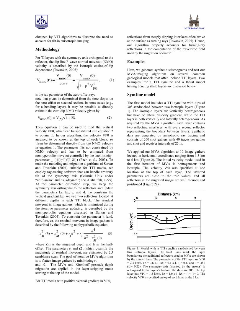
The first model includes a TTI syncline with dips of 30° sandwiched between two isotropic layers (Figure 1). The isotropic layers are vertically heterogeneous but have no lateral velocity gradient, while the TTI layer is both vertically and laterally heterogeneous. As required by the MVA algorithm, each layer contains two reflecting interfaces, with every second reflector representing the boundary between layers. Synthetic data are generated by anisotropic ray tracing and consists of 260 shot gathers with 40 traces per gather and shot and receiver intervals of 25 m.

We applied our MVA algorithm to 10 image gathers located at horizontal coordinates ranging from 1.5 km to 5 km (Figure 2). The initial velocity model used in the first iteration of MVA is homogeneous and isotropic. The velocity VP0 was specified at one location at the top of each layer. The inverted parameters are close to the true values, and all reflectors in the migrated image are well focused and positioned (Figure 2a).

Figure 1: Model with a TTI syncline sandwiched between two isotropic layers. The bold lines mark the layer boundaries; the additional reflectors used in MVA are shown by the thinner lines. The parameters of the TTI layer are VP0 = 2.3 km/s, kz = 0.6 s-1, kx = 0.1 s-1, �= 0.1, and �= -0.1 (�= 0.25). The symmetry axis (marked by the arrows) is orthogonal to the layers’s bottom; the dips are 30°. The top layer has VP0 = 1.5 km/s, kz = 1.0 s-1, kx = �= �= 0. The velocity VP0 is specified on top of each layer at the 1 km

If the symmetry direction velocity VP0 is known, the NMO velocities in the TTI layer can be inverted for the parameter (see equations 1 and 2). Although in the introduction this result is discussed for a homogeneous model because we estimate the velocity gradients by using image gathers at different depths and lateral positions. In contrast to VTI media, where the parameter (with a known VP0) can be found from dip-dependent NMO velocity, estimation of in TTI media generally requires using nonhyperbolic moveout. The relatively large offset-to-depth ratios (reaching two) used in the velocity analysis for the syncline model are sufficient to provide a constraint on .

Figure 2: (a) Final image of the model from Figure 1 obtained after MVA and prestack depth migration for TTI media. The estimated parameters of the first (subsurface) layer are kz = 0.99 s-1 and kx = �= �= 0. For the second layer, kz = 0.59 s-1, kx = 0.09 s-1, �= 0.09, and �= -0.11. For the third layer, kz = 0.29 s-1 and kx = �= �= 0. The error for each parameter varies from �0.01 to �0.02, if the depth picking error is assumed to be �5 m. Image gathers obtained (b) with the initial model parameters before MVA; (c) after six iterations of MVA for the first two layers; (d) after MVA for all three layers.

The improvements achieved by the MVA algorithm inreducing the residual moveout in image gathers areillustrated in Figures 2b-2d. Upon completion of theparameter estimation for all three layers, image gathers are flat throughout the model (Figure 2d).

To assess the stability of our MVA and migrationalgorithms, we added random uncorrelated Gaussian noise to the synthetic data set for the model from Figure 1. The signal-to-noise ration (S/N), measured as the ratio of the peak signal amplitude to the root-mean-square (rms) amplitude of the background noise, is close to two; the frequency bands of the signal and noise are identical (Figure 3a). The semblance maxima for most events in the presence of noise becomes less focused (Figure 3b), which enhances the tradeoff between the moveout parameters r1 and r2 in equation (3) (Tsvankin, 2005). However, since any pair of values (r1, r2) within the innermost semblancecontour provides nearly the same variance of migrateddepths, this tradeoff does not hamper the convergence

of the MVA algorithm. On the whole, despite the low S/N ratio, random noise does not significantly distort the MVA results (only the error in is non-negligible). Although the imaged reflectors are not as well focused as those on the noise-free section, they are clearly visible and correctly positioned (Figure 3c).

Since most anisotropic imaging algorithms used in industry are designed for VTI media, it is important to evaluate the influence of the tilted symmetry axis on the results of MVA and migration. To emulate a VTI processing sequence, we repeated the MVA without allowance for a tilted symmetry axis (i.e., the second layer was treated as VTI). After several iterations of parameter updating, the image gathers were largely flattened, and the image quality was only marginally inferior to that achieved for the true model (Figure 4). The parameters kz, and of the second layer, however, are distorted by the MVA algorithm, which has to flatten image gathers in the TTI layer with the incorrect tilt of the symmetry axis. It is interesting to note that the bestfit VTI model has an accurate value of the anellipticity parameter .

Figure 3: Influence of Gaussian noise on MVA and migration for the model from Figure 1. (a) One of the noise-contaminated shot gathers (the lateral coordinate is close to 2 km). (b) The semblance scan for the bottom of the TTI layer (the lateral coordinate is 1.9 km) computed as a function of the moveout coefficients r1 and r2 [equation (4)]. The maximum semblance is marked by the star. (c) The image obtained for the noise-contaminated data set. The estimated parameters of the first layer are kz = 1.06 s-1, kx = 0.01 s-1,

�= -0.01, and �= 0. For the second layer, kz = 0.56 s-1, kx = 0.11 s-1, �= 0.14, and �= -0.08. For the third layer, kz = 0.35 s-1, kx = 0.01 s-1, �= 0.02, and �= -0.02. The errors for each parameter vary from �0.03 to �0.05 under the assumption that the picking error for the noisy data is �20 m.

Figure 4: (a) Image of the model from Figure 1 obtained after applying MVA under the assumption that the second layer is VTI. The estimated parameters of the second layer used in the migration are kz = 0.53 s-1, kx = 0.12 s-1, �= 0.15, and �= -0.06 (�= 0.24). (b) The corresponding image gathers.

The ability of the VTI algorithm to compensate for the influence of tilt decreases for a larger relative thickness of the TTI syncline (Figure 5). Because of the more significant contribution of the interval traveltime in the TTI layer, the dipping reflectors in Figure 5 are misfocused and shifted in the vertical direction. Such artifacts can serve as an indication that the medium above the distorted reflectors may have a tilted symmetry axis.

Figure 5: Same as Figure 4a (i.e., the image obtained for the bestfit VTI model), but the thickness of the TTI layer from Figure 1 is increased by 200 m. The estimated parameters are kz = 0.52 s-1, kx = 0.12 s-1, �= 0.13, and �= -0.08 (�= 0.26).

Thrust model

The next test is performed for a simplified thrust model, which can be considered typical for complex tectonic process in fold-and-thrust belts, such as the Canadian Rocky Mountain Foothills and Himalaya Foothills. The model for these types of structures can be of bending shale layers with variable dips, which are upthrusted due to tectonic processes forming TTI layers. Here, we process synthetic data generated for a TTI thrust sheet (Figure 6) fashioned after the physical model of Leslie and Lawton (1996). This physical-modeling data set was used by Grechka et al. (2001) for anisotropic parameter estimation. The algorithm of Grechka et al. (2001), however, operates only with NMO velocities measured on conventional spreads and relies on several simplifying assumptions about the model.

Figure 6: TTI thrust sheet with variable dip for different blocks (0°, 30°, 55°, and 65°) and the symmetry axis (marked by the arrows) orthogonal to the sheet’s bottom. Except for the symmetryaxis direction, the parameters of all TTI blocks are the same: VP0 = 2.3 km/s, kz = 0.6 s-1, kx = 0.1 s-1, �= 0.1, and �= -0.1. The rest of the model is composed of isotropic layers. The subsurface (weathering) layer is thin (60 m) and has VP0 = 1.5 km/s, kz = 1.0 s-1, and kx = �= �= 0. The horizontal layer at the bottom of the model has VP0 = 3.5 km/s, kz = 0.3 s-1, and kx = �= �= 0.

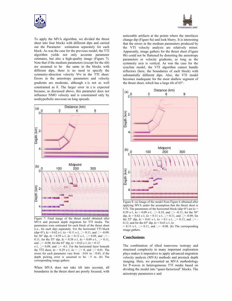
To apply the MVA algorithm, we divided the thrust sheet into four blocks with different dips and carried out the Parameter estimation separately for each block. As was the case for the previous model, the TTI algorithm yields not only accurate parameter estimates, but also a high-quality image (Figure 7). Note that if the medium parameters (except for the tilt) are assumed to be the same in the blocks with different dips, there is no need to specify thesymmetry-direction velocity VP0 in the TTI sheet. Errors in the anisotropy parameters and velocity gradients are moderate, although is not as well constrained as . The larger error in is expected because, as discussed above, this parameter does not influence NMO velocity and is constrained only by nonhyperbolic moveout on long spreads.

Figure 7: Final image of the thrust model obtained after MVA and prestack depth migration for TTI media. The parameters were estimated for each block of the thrust sheet (i.e., for each dip) separately. For the horizontal TTI block (dip=0°), kz = 0.62 s-1, kx = 0.11 s-1, �= 0.11, and �= -0.09; for 30° dip, kz = 0.59 s-1, kx = 0.12 s-1, �= 0.09, and �= -0.11; for the 55° dip, kz = 0.58 s-1, kx = 0.09 s-1, �= 0.11, and �= -0.08; for the 65° dip, kz = 0.62 s-1, kx = 0.12s-1, �= 0.09, and �= -0.1. For the horizontal layer beneath the TTI sheet, kz = 0.29 s-1, kx = �= 0, and �= 0.01. The errors for each parameter vary from �0.01 to �0.03, if the depth picking error is assumed to be �5 m. (b) The corresponding image gathers.

When MVA does not take tilt into account, all boundaries in the thrust sheet are poorly focused, with

noticeable artifacts at the points where the interfaces change dip (Figure 8a) and look blurry. It is interesting that the errors in the medium parameters produced by the VTI velocity analysis are relatively minor. Apparently, image gathers for the thrust sheet (Figure 8b) could not be flattened by distorting the anisotropy parameters or velocity gradients, as long as the symmetry axis is vertical. As was the case for the syncline model, the VTI algorithm cannot handle reflectors (here, the boundaries of each block) with substantially different dips. Also, the VTI model becomes inadequate for the most shallow segment of the thrust sheet, which has a large tilt of 65°.

Figure 8: (a) Image of the model from Figure 6 obtained after applying MVA under the assumption that the thrust sheet is VTI. The parameters of the horizontal block (dip=0°) are kz = 0.59 s-1, kx = 0.09 s-1, �= 0.19, and �= -0.11; for the 30° dip, kz = 0.62 s-1, kx = 0.11 s-1, �= 0.11, and �= -0.09; for the 55° dip, kz = 0.61 s-1, kx = 0.1 s-1, �= 0.13, and �= -0.12; and for the 65° dip, kz = 0.63 s-1, kx= 0.13 s-1, �= 0.11, and �= -0.08. (b) The corresponding image gathers.

Conclusions

The combination of tilted transverse isotropy and structural complexity in many important exploration plays makes it imperative to apply advanced migration velocity analysis (MVA) methods and prestack depth imaging. Here, we presented an MVA methodology for P-waves in heterogeneous TTI media based on dividing the model into “quasi-factorized” blocks. The anisotropy parameters and

in each block are constant, while the symmetry-direction velocity VP0 represents a linear function of the spatial coordinates and is described by the vertical (kz) and lateral (kx) gradients. To reduce the uncertainty in parameter estimation, the symmetry axis in each block or layer is taken to be orthogonal to the reflector at the bottom of the block. Since reflectors may have arbitrary shape, the symmetry-axis orientation generally varies in space, which means that blocks are not fully factorized. On the other hand, the symmetry-axis direction is always orthogonal to the reflector and fixed in TI factorized media.

Our algorithm represents an extension to TTI media of the methodology developed by Sarkar and Tsvankin (2004) for vertical transverse isotropy (VTI). MVA is combined with Kirchhoff prestack depth migration based on anisotropic ray tracing for heterogeneous TI media with arbitrary tilt. Parameter estimation is performed in a layer-stripping mode starting at the surface, with the symmetry-direction velocity VP0

either specified at a single point in each block or assumed to be continuous in the vertical direction. To estimate the vertical gradient kz, we use image gathers for at least two reflectors at different depths within each block.

The MVA and migration algorithms were tested ondifferent typical TTI models like syncline and a bending TTI layer (thrust sheet). For all these type models, we were able to accurately reconstruct the velocity gradients kz and kx throughout the medium and the anisotropy parameters and in the TTI blocks. The migrated sections computed with the estimated velocity model are practically indistinguishable from the true images, with good focusing and positioning of reflectors beneath the TTI formations.

To assess the influence of tilt on image quality, wemigrated the data with the VTI model (i.e., with zero tilt) that has the correct values of VP0, kz, kx, and . Although tilt in our first model (the syncline) is moderate (30°), setting it to zero results in significant misfocusing and mispositioning of reflectors. The inaccuracy of the VTI velocity field also manifests itself through substantial residual moveout in image gathers.

In order to emulate a complete VTI processing sequence applied to TTI media, we performed MVA without allowance for a tilted symmetry axis to obtain the “best-fit” VTI model. The MVA algorithm can achieve partial flattening of image gathers with the incorrect tilt, but at the expense of distorting the medium parameters, especially and (although the value of remains accurate). Such artificial adjustments in and improve image quality, although migrated sections typically are inferior to those generated with the TTI model. Also, the ability

of the VTIbased algorithm to compensate for the influence of tilt decreases for more complicated models and TTI layers with relatively large thickness or strong anisotropy.

References

Alkhalifah, T., 1995, Efficient synthetic-seismogramgeneration in transversely isotropic, inhomogeneous media; Geophysics, 60, 1139-1150.

Dewangan, P. and Tsvankin, I., 2006a, Modeling and inversion of PS-wave moveout asymmetry for tilted TI media: Part 1 – Horizontal TTI layer; Geophysics, 71, D107-D121.

Dewangan, P. and Tsvankin, I., 2006b, Modeling and inversion of PS-wave moveout asymmetry for tilted TI media: Part 2 – Dipping TTI layer; Geophysics, 71, D123- D134.

Grechka, V., Pech., A., Tsvankin, I. and Han, B., 2001, Velocity analysis for tilted transversely isotropic media: A physical modeling example; Geophysics, 66, 904-910.

Kumar, D., Sen, M. K., and Ferguson, R. J., 2004,Traveltime calculation and prestack depth migration in tilted transversely isotropic media; Geophysics, 69, 37-44.

Leslie, J. M. and Lawton, D. C., 1996, Structural imaging below dipping anisotropic layers: Predictions from seismic modeling; 66th SEG Meeting, Denver, USA, Expanded Abstracts, 719-722.

Pech, A., Tsvankin, I. and Grechka, V., 2003, Quartic moveout coefficient: 3D description and application to tilted TI media; Geophysics, 68, 1600-1610.

Sarkar, D. and Tsvankin, I., 2004, Migration velocityanalysis in factorized VTI media; Geophysics, 69, 708-718.

Sarkar, D. and Tsvankin, I., 2006, Anisotropic migration velocity analysis: Application to a data set from West Africa; Geophysical Prospecting, 54, 575-587.

Tsvankin, I., 2005, Seismic signatures and analysis of Reflection data in anisotropic media, 2nd edition; Elsevier Science Publishing Co.

Vestrum, R., Lawton, D. C. and Schmid, R., 1999, Imaging structures below dipping TI media; Geophysics, 64, 1239- 1246.

Acknowledgments

We are grateful to the A(nisotropy)-Team of the Center for Wave Phenomena (CWP), Colorado School of Mines (CSM), and other colleagues at CWP for fruitful discussions. L. B. thanks the Department of Science and Technology, Govt. of India, for awarding him BOYSCAST Fellowship and V. P. Dimri, Director of the National Geophysical Research Institute, Council of Scientific and Industrial Research, for granting him permission to pursue postdoctoral research in CWP. This work was partially supported by the Consortium Project on Seismic Inverse Methods for Complex Structures at CWP.