
III. CHARACTER MODELING FROM SYNTHETIC SEISMOGRAMS 8 …
87
SYNTHETIC SEISMOGRAMS AND CHARACTER MODELING AN AID TO THE DETERMINATION OF THE EARTH'S STRUCTURE FROM RAYLEIGH WAVES by RICHARD L. CRIDER, B.S. A THESIS IN GEOSGIENCES Submitted to the Graduate Faculty of Texas Tech University in Partial Fulfillment of the Requirements for the Degree of MASTER OF SCIENCE Approved Accepted Dean of the Graduad^e" School May, 1980
Transcript of III. CHARACTER MODELING FROM SYNTHETIC SEISMOGRAMS 8 …

SYNTHETIC SEISMOGRAMS AND CHARACTER MODELING
AN AID TO THE DETERMINATION OF THE EARTH'S
STRUCTURE FROM RAYLEIGH WAVES
by
RICHARD L. CRIDER, B.S.
A THESIS
IN
GEOSGIENCES
Submitted to the Graduate Faculty of Texas Tech University in
Partial Fulfillment of the Requirements for
the Degree of
MASTER OF SCIENCE
Approved
Accepted
Dean of the Graduad^e" School
May, 1980

7 w
ACKNOWLEDGMENTS
I am very grateful to Professor D. H. Shurbet for
his direction of this thesis.
My appreciation is expressed to Sunmark Exploration
Company, Irving, Texas, for permitting me to use their
computer facilities, without which this study would not
have been possible.
11
CONTENTS
ACKNOWLEDGEMNTS ii
LIST OF FIGURES iv
I. INTRODUCTION 1
II. THEORY 3
III. CHARACTER MODELING FROM SYNTHETIC
SEISMOGRAMS 8
IV. CORRELATION OF SYNTHETIC SEISMOGRAMS
WITH EARTHQUAKE SEISMOGRAMS 41
V. CONCLUSIONS 76
VI. RECOMMENDATIONS 77
LIST OF REFERENCES 79
111
LIST OF FIGURES
FIGURE
1. Configuration of the basic Earth model
2. Synthetic seismograms generated for the basic model Ml and the model M2 . . .
5.
6.
3. Synthetic seismograms generated for the models M3 and M4
4. Synthetic seismograms generated for the models M5 and M6
Synthetic seismograms generated for the models M7 and M8
Synthetic seismograms generated for the models M9 and MlO
7. Synthetic seismograms generated for the models Mil and M12
8. Synthetic seismograms generated for the models M13 and M14
9. Theoretical dispersion data for the basic model Ml
10. Theoretical dispersion data for the model M2
11. Theoretical dispersion data for the model M3
12. Theoretical dispersion data for the model M4
13. Theoretical dispersion data for the model M5
14. Theoretical dispersion data for the model M6
15. Theoretical dispersion data for the model M7
16. Theoretical dispersion data for the model M8
17. Theoretical dispersion data for the model M9
PAGE
9
11
12
13
14
15
16
17
18
19
20
21
22
23
24
25
26
IV
FIGURE
1 8 .
1 9 .
2 0 .
2 1 .
2 2 .
2 3 .
2 4 .
2 5 .
2 6 .
2 7 .
2 8 .
PAGE
Theoretical dispersion data for the model MlO. 27
Theoretical dispersion data for the model Mil. 28
Theoretical dispersion data for the model M12. 29
Theoretical dispersion data for the model M13. 30
Theoretical dispersion data for the model M14. 31 (•
Synthetic seismograms generated for models M15 and M16 35
Synthetic seismogram generated for model M17 . 36
Theoretical dispersion data for the model M15. 37
Theoretical dispersion data for the model M16. 38
Theoretical dispersion data for the model M17. 39
Long period vertical components of seismograms for Event 1 and Event 2 43
29. Locations of the epicenters for Event 1 and Event 2 44
30. Cross correlation function for Event 1 correlated with the synthetic seismogram for basic model Ml 46
31. Cross correlation function for Event 1 correlated with the synthetic seismogram for the model M2 47
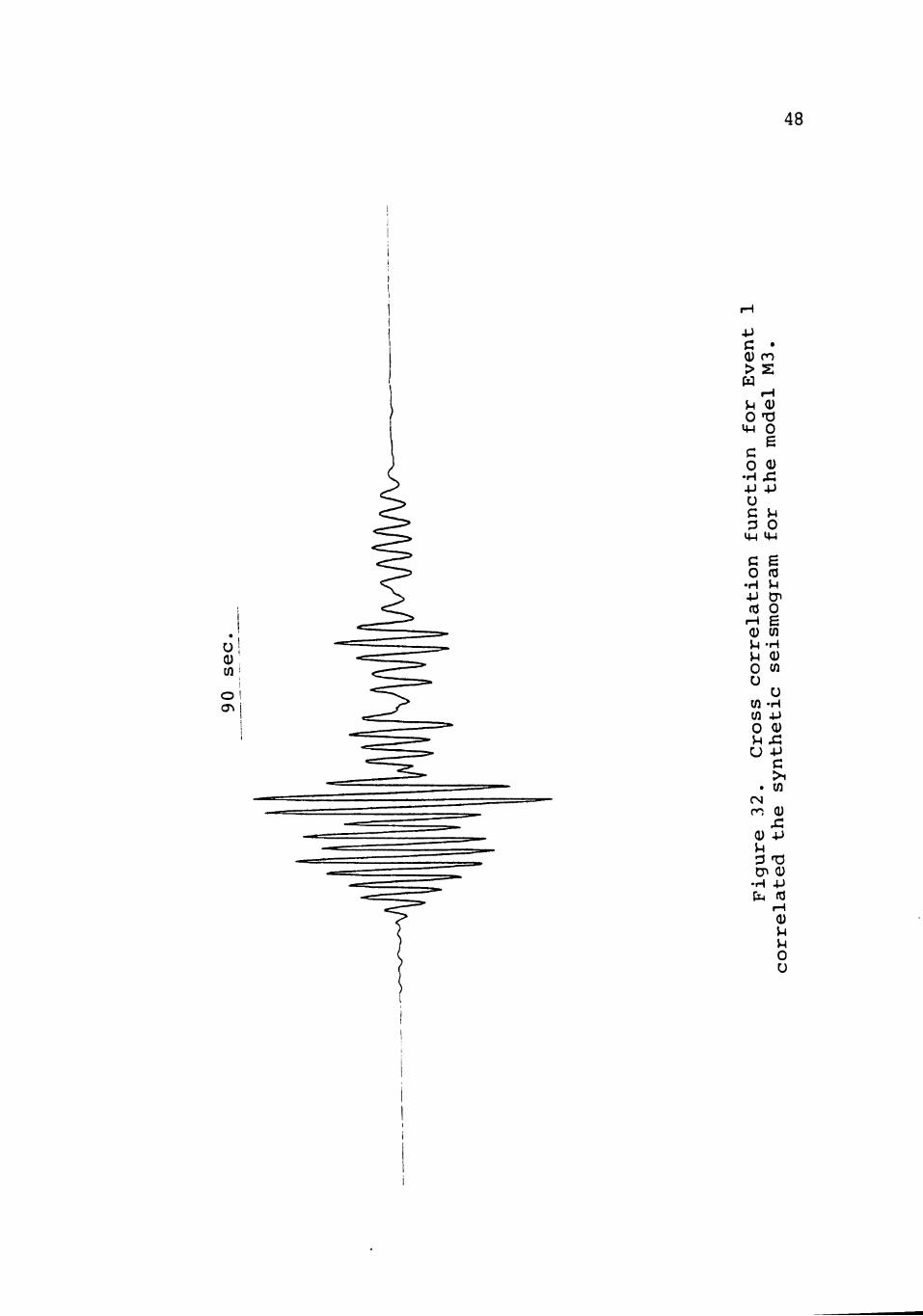
32. Cross correlation function for Event 1 correlated with the synthetic seismogram for the model M3 48
33. Cross correlation function for Event 1 correlated with the synthetic seismogram for the model M4 49
34. Cross correlation function for Event 1 correlated with the synthetic seismogram for the model M5 50
35. Cross correlation function for Event 1 correlated with the synthetic seismogram for the model Mb 51
V

FIGURE PAGE
36. Cross correlation function for Event 1 correlated with the synthetic seismogram for the model M7 52
37. Cross correlation function for Event 1 correlated with the synthetic seismogram for the model M8 53
38. Cross correlation function for Event 1 correlated with the synthetic seismogram for the model M9 54
39. Cross correlation function for Event 1 correlated with the synthetic seismogram for the model MlO 55
40. Cross correlation function for Event 1 correlated with the synthetic seismogram for the model Mil 56
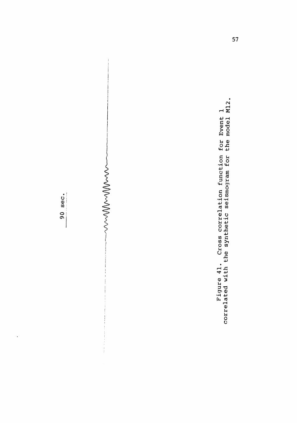
41. Cross correlation function for Event 1 correlated with the synthetic seismogram for the model M12 57
42. Cross correlation function for Event 1 correlated with the synthetic seismogram for the model M13 58
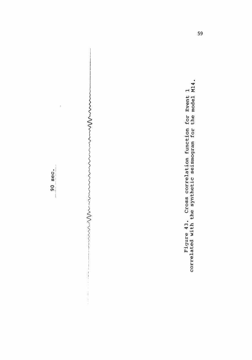
43. Cross correlation function for Event 1 correlated with the synthetic seismogram for the model M14 59
44. Cross correlation function for Event 2 correlated with the synthetic seismogram for the basic model Ml 61
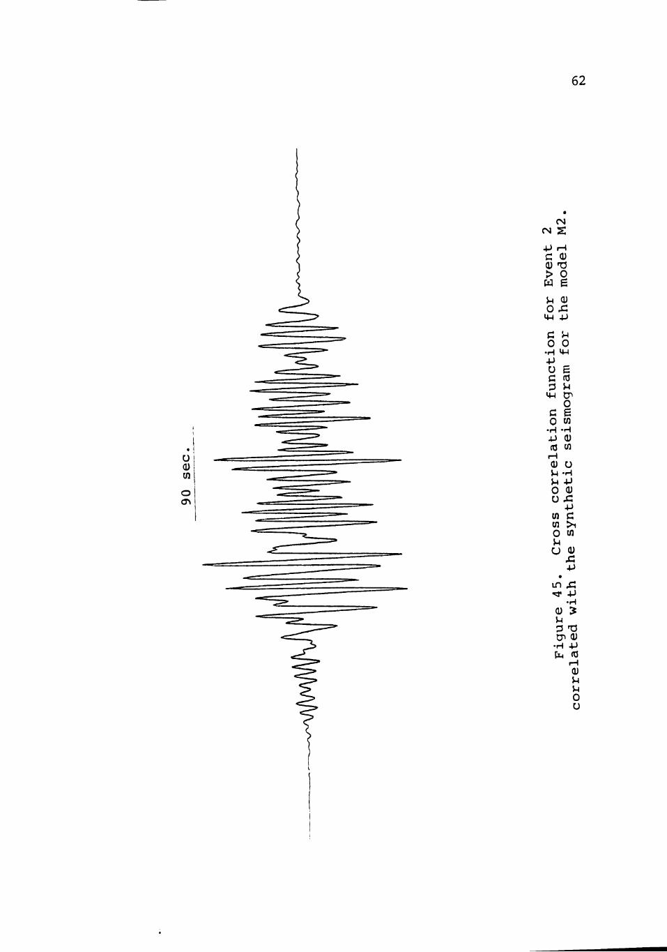
45. Cross correlation function for Event 2 correlated with the synthetic seismogram for the model M2 62
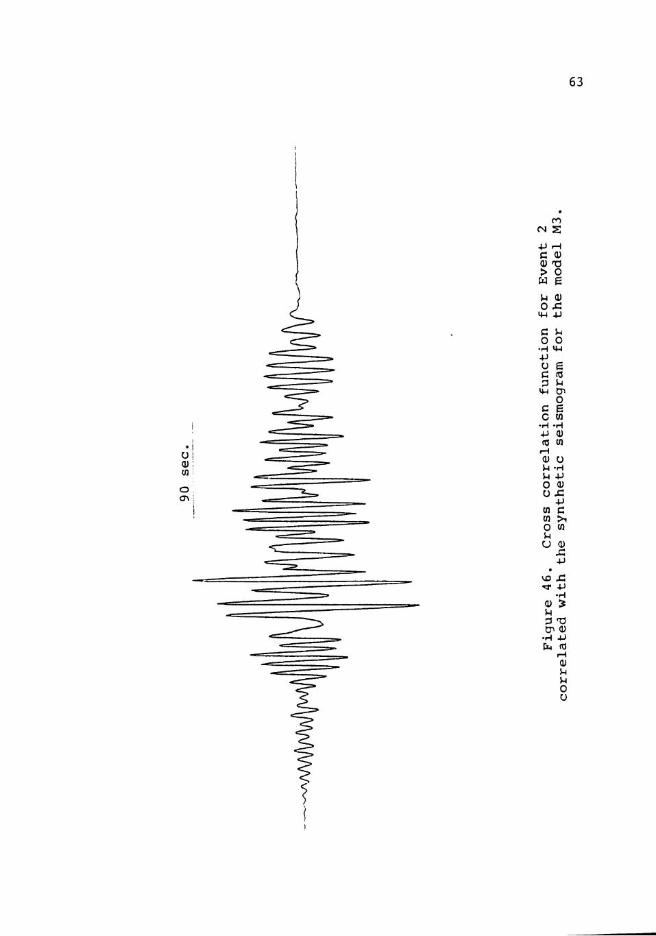
46. Cross correlation function for Event 2 correlated with the synthetic seismogram for the model M3 6 3
47. Cross correlation function for Event 2 correlated with the synthetic seismogram for the model M4 6 4
vi

FIGURE PAGE
48. Cross correlation function for Event 2 correlated with the synthetic seismogram for the model M5 65
49. Cross correlation function for Event 2 correlated with the synthetic seismogram for the model M6 66
50. Cross correlation function for Event 2 correlated with the synthetic seismogram for the model M7 67
51. Cross correlation function for Event 2 correlated with the synthetic seismogram for the model M8 68
52. Cross correlation function for Event 2 correlated with the synthetic seismogram for the model M9 69
53. Cross correlation function for Event 2 correlated with the synthetic seismogram for the model MlO 70
54. Cross correlation function for Event 2 correlated with the synthetic seismogram for the model Mil 71
55. Cross correlation function for Event 2 correlated with the synthetic seismogram for the model M12 72
56. Cross correlation function for Event 2 correlated with the synthetic seismogram for the model M13 73
57. Cross correlation function for Event 2 correlated with the synthetic seismogram for the model M14 74
Vll

CHAPTER I
INTRODUCTION
Direct and indirect modeling techniques are commonly
used in the determination of the earth's interior from
seismic surface wave dispersion. The most widely used
modeling technique is an indirect trial-and-error procedure
in which dispersion is computed for models in an effort to
duplicate observed dispersion. Indirect modeling has been
applied to Rayleigh and Love wave phase and group velocity
dispersion in the fundamental and higher modes (Dorman and
Ewing, 1962; Dorman et al., 1960). Theoretically exact
methods for the computation of dispersion have been pre
sented by Haskell (1953) and by Alterman and others (1959).
Direct modeling is used to determine the correspond
ing earth model from observed surface wave dispersion
(Dorman and Ewing, 1962; McEvilly, 1964; Braile and Keller,
1975; Bloch et al., 1969). Current direct modeling tech
niques place stringent requirements on data quality (Braile
and Keller, 1975) and these requirements limit the appli
cation of direct modeling.
Character modeling is a type of direct modeling which
utilizes the theoretical computations aspect of indirect
modeling to make a direct determination of earth structure
from surface wave dispersion. Character modeling is accom
plished by comparing synthetic seismograms for earth models
with earthquake seismograms. The identification of similar
character between the synthetic and true seismograms pro
vides a direct determination of the earth model.
Character modeling is an important tool in exploration
seismology. The synthesis of dispersed wave trains is also
well known (Sato, 1960; Brune et al., 1960; Aki, 1960), but
there has been no direct extension of character modeling
into earthquake seismology.
The purpose of this paper is to present the results
obtained from the application of character modeling to the
determination of a model for the earth's crust beneath
Mexico. A rapid method for the synthesis of dispersed waves
is presented. Variations in seismogram character are il
lustrated by the computation of synthetic seismograms for
a basic model and for permutations of the basic model. The
suite of synthetic seismograms produced are compared to
Rayleigh waves from two earthquakes in Mexico to determine
a crustal model.
The technique for the analysis of surface wave disper
sion presented in this paper is not intended to replace
other direct or indirect modeling tactics. This procedure
is presented as a means of enhancing the other techniques by
more effectively utilizing current data processing methods.

CHAPTER II
THEORY
The behavior of sound waves in the earth is described
by the one-dimensional time dependent wave equation
9^ y(x,t) _ 1 8^ y(x,t) ,,, 2 2~ 2 ^•^'
dx v^ 9t
where v is the velocity of propagation of the disturbance
y(x,t), x is distance, and t is time. A solution to the
wave equation is expressed as
y(x,t) = A 6 '' -' = ' (2)
where A is the amplitude, w is the angular frequency, and
k is the propagation constant or wave number.
Equation (2) represents a propagating wave with a well-
defined frequency w. However, if the frequency is to re
main well-defined, the wave train y(x,t) must be infinite
in length (Marion, 1967). For y(x,t) to be finite in
length, the wave train must be represented as the super
position of an infinite number of wave functions with
unique frequencies and wave numbers differing from each

other by some small amount Aw and Ak. The amplitude of the
function y(x,t) will then be a function of the wave number
and y(x,t) is expressed as
(x,t) = r A(k) ei''"*=-'^^'dx. (3)
The superposition of these wave functions is demon
strated by assuming that two of the functions have the form
,, / x.\ TV i(a),t-kTx) y, (x,t) = A e ' 1 1
y2(x,t) = A e^'"2*-'^2=^'
where w- = o), + Aw and k^ = k + Ak and, for simplicity,
the amplitude A is the same for each function. Summing
these two functions and retaining only the real parts of
the complex result, the total wave function is obtained.
,./ i.> 17V _„ (Aw) t-(Ak) x „ L ^ Awv. ,, ,Ak, I ,., y(x,t) = 2A cos - —j^ — cos (w+ -2-) t-(k+-2-) x (4)
Equation (4) for the resultant wave function is comprised
of two factors: the first represents an envelope, while
the second represents an average component wave.
The velocities of propagation of the envelope and com
ponent wave are determined by requiring that the arguments
of the two cosine terms, the phase, remain constant.

This requirement is expressed as
r(Aw)t - (Ak)x]_ . . ,, |_ 2 J •'^ ^^ envelope.
and dl(w+ "J") t - (k + "J") x = 0 for the component wave
Taking the derivatives we find, if we assume that w+ Aw
and w are not much different from each other, the results
(Aw)dt - (Ak)dx = 0 for the envelope,
and wdt - kdx = 0 for the component wave.
The velocities then are determined to be
V-dx dt
Aw Ak for the envelope.
= «^ TT - dx _ w. "• " 2 - dt - k for the component wave
The velocity v is known as the group velocity and the com
ponent wave velocity v^ as the phase velocity. The group
velocity is the velocity with which the energy in the wave
is transmitted.
The wave function described by equation (3) then is a
packet of waves whose velocities are a function of frequen
cy. This dependency of velocity upon frequency causes a
distortion of the wave form, a phenomenon known as
dispersion.
The displacement of the wave function at a particular
distance x, arbitrarily chosen as x = 0, is described by
the equation
y(t) = r A(w) e^'^^dw. (5)
This function can be computed by an inverse Fourier
Transform when the spectral distribution A(w) is known
(Marion, 1967).
Synthetic seismograms may be generated by approxi
mating the spectral distribution of the function y(t) by
a simple rectangle of the form
•TV / \ -i'l' (W) J
A(w) = e and A(w) = 1 (6)
for all frequencies in a band between w, and w^ (Aki, 1960).
Here (J) (w) = ^ ^ + *,- (w) (7) ^ Vw J in
where A is distance, C(w) is phase velocity, and <t> - (w) is
instrumental phase delay. The spectral distribution func
tion is then defined by the phase velocities of the frequen
cy band of interest.
Phase velocities for the frequency band used were
computed using Haskell's (1953) method. The computations
were accomplished using a FORTRAN IV computer program made
available to Texas Tech University by the University of
Texas at Dallas. The original program was modified to run
on the Sunmark Exploration Company's RDS 500 computer. The
spectral distribution was computed in equations (6) and (7)
for arbitrary distance. Since most seismograms reflect
particle velocity, the synthetic seismograms were computed
for velocity rather than displacement by taking the time
derivative of both sides of equation (6).
CHAPTER III
CHARACTER MODELING FROM SYNTHETIC SEISMOGRAMS
The basic earth model used in this study is shown in
Figure 1. The crustal section of this model is 41.3 km.
thick and is comprised of single-layer sedimentary and
granitic portions and a multi-layer basaltic portion. The
mantle section of the model is a generalized model common
to many areas of the world (Dorman et al., 1960; Brune and
Dorman, 1963) ; it approxim.ates a Gutenberg model. Vari
ations in this model for this study are restricted to the
crustal section. Additionally, synthetic seismogram
generation is limited to the Rayleigh mode since this
is the m.ost commonly recorded surface wave mode.
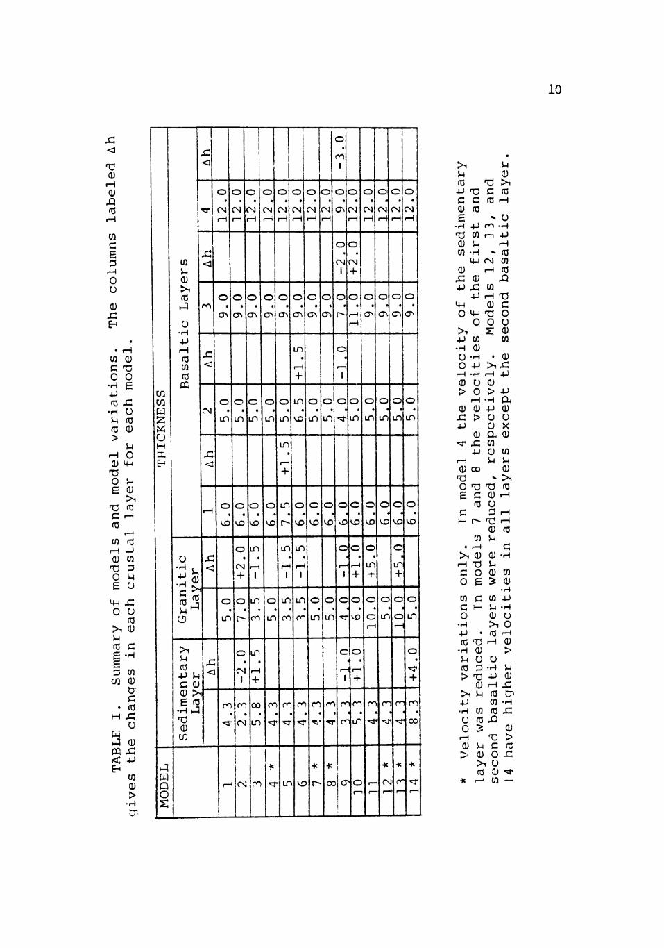
Synthetic seismograms for the basic model and thirteen
variations of the model are shown in Figures 2 to 8. The
theoretical phase and group velocity data for these syn
thetics are given in Figures 9 to 22. These seismograms
and data will be referred to as Ml through M14. A summary
of the model variations is given in Table I.
The synthetic seismograms were computed using a FOR
TRAN IV program written for the Raytheon RDS 500 computer.
This program accepts frequency, phase velocity, and arbi-
8

h
^ . 3
5.C
6 .0
5 .0
9 .0
12.0
30 .0
20 .0
35 .0
50 .0
^ 4 , 0
0 .0
V
p
^ . 9 3
6 . 1 ^
6.52
6.65
6.72
6.77
8.27
7.98
7.82
8.02
8.11
8.50
V s
2 .85
3.^9
3 .73
3.79
3.83
3.86
h.6k
hr.kS
^ .39
4 .50
^'55
^.77
p
2.62
2 .65
2 .87
2 .95
3 .0^
3 . 1 ^
3.57
3.69
3 .7^
3.79
3.80
3.69
Figure 1. Configuration of the basic Earth model. Layer thickness H is given in km, the compressional and shear velocities Vp and Vs are given in km/sec, and the density p is given in gm/cc. The dashed line indicates the boundary between the 41.3 km-thick crust and the mantle.
10
<
T : 0) rH (U n (C
i H
en c £ 3
r H
0 u 0) x: EH
• m c 0
•H 4J
• i H (U T3 0 E
fc x : •H ^ (t! >
i H
Q) T3 0 E
13 C fC
U) n-l
0) 13 0 E
u (T3 Q)
U 0
M-i
5-1 Q) >^ tC
r H
r H
fd 4J cn p M 0
IH £ 0
> i >-( 03 p 3 W
• H
w J
u fC a; c
• H
cn Q;
cr c nJ
r o (U
CC X I <: EH
4J
w 0) >
•H
C/i Ul H 2
M M - t
EH
J
Q O S
(0
M (U > 1 03 J
O • H
i H 03 cn 03 ffi
o • H , ,
• H <" C ^
> . S-< 03 -P >-l C Q)
E 03 •H J
Sed
1 x: <
^
s: <
m
x: < j
CN
o
CN i H
O
O^
o
IT)
JC < ]
r H
x: «-i
, r <
o
VO
o
IT)
m
' 3 '
r-H
o
CM r H
O
a^
o
IT)
o
VO
o •
CN
+ O
I ^
c •
OS 1
m
CN
O
CN r H
o
CTi
O
LD
O
VO
I D
• i H 1
tn
ro
I D
• r—1 +
c»
ID
1
CM m
o
CN
•"
o
cr.
o
i n
o
VO
o
i n
m
"^
«
"^
o
fs i H
O
<y\
o
i n
i n •
r—1
+
i n
r^
i n •
r H 1
i n
ro
m
"^
I T
O
rvj r H
o
<T.
in • r H
+ i n
VD
o
VO
i n •
r H
1
in
m
r^
•«5"
VO
o
CN r H
C
<r>
o
i n
o
VO
o
i n
0 0
<5'
•K
r-
o
CN r H
o
o •
ro 1
O
cr.
o •
CN
1
o
cr> c~-
c
in
o
VO
o
i n
r^
' ^
•a
a
o
r—>
1
o
^
o
VO
o
r—'
1
o
•^
<z
1 —
1
c
r-
1
) G
O
C J r H
O
« CN
+ O
r-H r H
o
CN r H
o
<ys
o
in
o
VO
o •
r-H
o
in
o
VO
o •
i n + + o
VO
O
» r-H
+
ro
i n
o
o
o t—1
ro
•>:l<
r— f —
o
CN r H
O
cr.
o
i n
o
VO
o •
i n
r^
^
*
CN ( r—
o
CN r H
o
c\
o
in
o
VO
o I
i n + o
i
O r-H
r
• T
•K
r < r —
o
CN r H
O
<r.
o
i n
o
VO
o •
i n
c •
+
ro
CO
•K
»T r-H
>1 5-1 03 4-1 no C C 0) fO E
•H 4-)
13 cn
cn -H
x: OJ -p x:
-p
o ^ o
> i 4-> cn •H Q) O -H O -P
rH -H (D U > 0
rH
x: > 4J
j j
(U 00 13 O 13 £ C
03 C M r-
cn • rH
rH 13 C O O E
cn c C H-o
•H -P • fC 13
•H (U P U 03 P > 1 ;
0) >^ P •P •H cn U 03 O 5
rH d) u > CJ
> 1 03
•K r-J
u
13 > i C 03 fO rH
- O ro -H r-i 4J
rH •> 03
rvj cn iH 03
cn ,-i Q)
13 O
13 C O U 0) cn
rH 4-1
> -p •H a. -P Q) U O CD ><
a Q) cn 0) cn u u
Q) - > i
13 03 CD T-^ u
13 rH (D 03 P
C o; -H p Oj cn
•H cn 4-> P -H Q) U > i O 03 r-^
U •H 4J
p
a; .H x: 03 C7> cn - H 03 £
XJ a;
13 > C 03 o sz o cn -^

11
fV^'
90 sec.
Figure 2. Synthetic seismograms generated for the basic model Ml and the model M2 having a thinned sedimentary layer and a thickened granitic layer. The theoretical dispersion data for these models are given in Figures 9 and 10, respectively.

12
90 sec.
Figure 3. Synthetic, seismograms generated for models M3 and M4. M3 has a thickened sedimentary layer and a thinned granitic layer. The sedimentary layer velocity was reduced in M4. The theoretical dispersion data for these models are given in Figures 11 and 12, respectively.

13
90 sec.
Figure 4. Synthetic seismograms generated for models M5 and M6. Each model has a thinned granitic layer and a thickened basaltic layer. The theoretical dispersion data for these models are given in Figures 13 and 14, respectively.

14
90 sec.
Figure 5. Synthetic seismograms generated for models M7 and M8. These models have reduced velocities in either the second basaltic layer (M7) or in the first and second basaltic layers (M8). The theoretical dispersion data for these models are given in Figures 15 and 16, respectively.

15
90 sec.
Figure 6. Synthetic seismograms generated for models M9 and MlO. M9 has a thinned crust (33.3 km). MlO has a thickened crust (45.3 km). The theoretical dispersion data for these models are given in Figures 17 and 18, respectively.
16
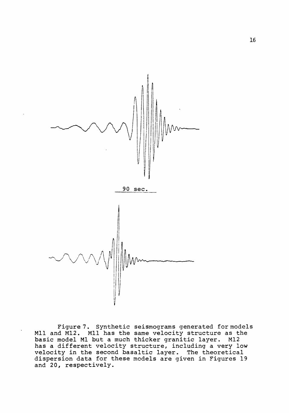
90 sec
Figure 7. Synthetic seismograms generated for models Mil and M12. Mil has the same velocity structure as the basic model Ml but a much thicker granitic layer. M12 has a different velocity structure, including a very low velocity in the second basaltic layer. The theoretical dispersion data for these models are given in Figures 19 and 20, respectively.

17
90 sec.
Figures. Synthetic seismograms generated for models M13 and M14. These models are identical to M12 with the exception of a thickened granitic layer in M13 and a thickened sedimentary layer in M14. The theoretical dispersion data for these models are given in Figures 21 and 22, respectively.

18
MODEL I
4.5-
4.0-
o a>
3.5
u o - J >
3.0-
H
4.3
5.0
6.0
5.0
9.0
12.0
Vp
4.93
6.14
6.52
6.65
6.72
6.77
Vs
2.85
3.49
3.73
3.79
3.83
3.86
P
2.62
2.65
2.87
2.95
3.04
3.14
PHASE VELOCITY
GROUP VELOCITY
10 20 30 40 50
PERIOD (sec)
Figure 9. Theoretical dispersion data for the basic model Ml.
19
4.5-
MOOEL 2
H
2.3 7.0
6.0
5.0
9.0
12.0
Vp
4.93 6.14
6.52
6.65
6.72
6.77
Vs
2.85 3.49
3.73
3.79
3.83
3.86
P 1 2.62 2.65
2.87
2.95
3.04
3.14
4.0-u
£
>•
h: o o - J UJ >
3.5-
PHASE VELOCITY
3.0-
GROUP VELOCITY
- r — 10 20^ 'zo 40* 50
PERIOD (sec)
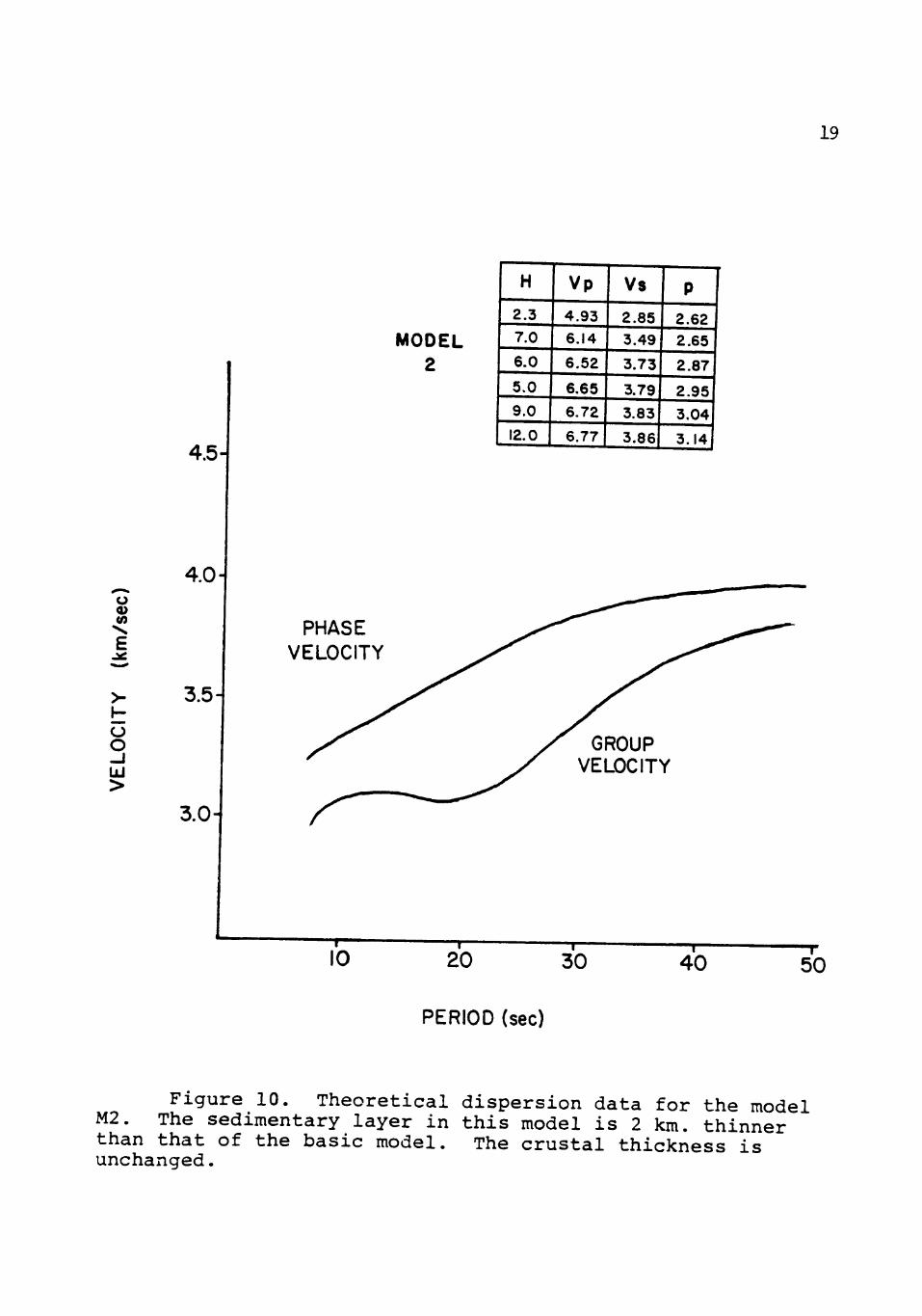
Figure 10. Theoretical dispersion data for the model M2. The sedimentary layer in this model is 2 km. thinner than that of the basic model. The crustal thickness is unchanged.

20
MODEL 3
4.5
4.0-
o CO PHASE
VELOCITY
3.5-
o o -J UJ >
3.0-
GROUP VELOCITY
PERIOD (sec)
'h^^^f^/^\ Theoretical dispe: M3. The sedimentary layer in thir^^i"? ^^^^ -°^ ^^^ " odel than that of the baLc m odel ? 5.\^ " ^ ^ ^ ' ^ l ^ ^ ^ ^ ^ ^ ^ ^ r unchanged.

21
4.5
4.0
o
E 2C
O O
UJ >
3.5-
3.0
MODEL 4
H 4.3
5.0
6.0
5.0
9.0
12.0
Vp 4.13
6.14
6.52
6.65
6.72
6.77
Vs 2.38
3.49
3.73
3.79
3.83
3.86
P 2.62
2.65
2.87
2.95
3.04
3.14
PHASE VELOCITY
GROUP VELOCITY
10 20 30 40 50
PERIOD (sec)
Figure 12. Theoretical dispersion data for the model M4. The velocity in the sedimentary layer is reduced from that of the basic model.
22
4.5
4.0-
o
>•
O O _l UJ >
3.5
3.0-
MODEL 5
H
4.3
3.5
7.5
5.0
9.0
12.0
Vp 4,93
6.14
6.52
6.65
6.72
6.77
Vs 2.85
3.49
3.73
3.79
3.83
3.86
P 2.62
2.65
2.87
2.95
3.04
3.14
PHASE VELOCITY
GROUP VELOCITY
10 20 30 40 50
PERIOD (sec)
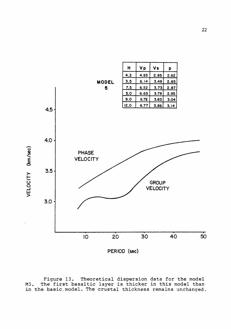
Figure 13. Theoretical dispersion data for the model M5. The first basaltic layer is thicker in this model than in the basic.model. The crustal thickness remains unchanaed.

23
4.5"
4.0-
o (A
E
>-
o o _l UJ >
3.5-
3.0-
MODEL 6
H 4.3
3.5
6.0
6.5
9.0
12.0
Vp 4.93
6.14
6.52
6.65
6.72
6.77
Vs 2.85
3.49
3.73
3.79
3.83
3.86
P 2.62
2.65
2.87
2.95
3.04
3.14
PHASE VELOCITY
GROUP VELOCITY
10 20 30 40 50
PERIOD (sec)
Figure 14. Theoretical dispersion data for the model M6. The second basaltic layer is thicker in this model than in the basic model. The crustal thickness remains unchanged.

24
4.5-
4.0-o a>
£
>-
o - I UJ >
3.5-
3.0-
MODEL 7
H
4.3
5.0
6.0
5.0
9.0
12.0
Vp
4.93
6.14
6.52
6.25
6.72
6.77
Vs
2.85
3.49
3.73
3.61
3.83
3.86
P
2.62
2.65
2.87
2.85
3.04
3.14
PHASE VELOCITY
GROUP VELOCITY
10 20 30 40 50
PERIOD (sec)
Figure 15. Theoretical dispersion data for the model M7. The second basaltic layer is replaced by a low velocity layer of the same thickness.

25
4.5-
4.0-o
MODEL 8
H
4.3
5.0
6.0
5.0
9.0
12.0
Vp
4.93
6.14
6.40
6.25
6.72
6.77
Vs
2.85
3.49
3.66
3.61
3.83
3.86
P 2.62
2.65
2.87
2.85
3.04
3.14
PHASE VELOCITY
3.5-
3 UJ >
3.0
GROUP VELOCITY
10 20 30 40 50
PERIOD (sec)
Figure 16. Theoretical dispersion data for the model M8. The velocities in the first and second basaltic layers are reduced.

26
4.5-
4.0-o (A
o o - i UJ >
3.5
3.0-
MODEL 9
H
3.3
4.0
6.0
4.0
7.0
9,0
Vp
4.93
6.14
6.40
6.25
6.72
6.95
Vs
2.85
3.49
3.66
3.61
3.83
3.96
P 2.62
2.65
2.87
2.85
3.04
3.14
PHASE VELOCITY
GROUP VELOCITY
10 20" 30 40 50
PERIOD (sec)
Figure 17. Theoret ica l d ispers ion data for the model M9. The c r u s t a l th ickness of t h i s model i s 33.3 km.
27
MODEL 10
4.5-
4.0
E
3.5"
u o UJ >
3.0-
H
3.3
4.0
6.0
4 .0
7.0
9.0
Vp
4.93
6.14
6.52
6.65
6.72
6.77
Vs
2.85
3.49
3.73
3.79
3.83
3.86
P
2.62
2.65
2.87
2.95
3.04
3.14
PHASE VELOCITY
GROUP VELOCITY
10 20 30 40 50
PERIOD (sec)
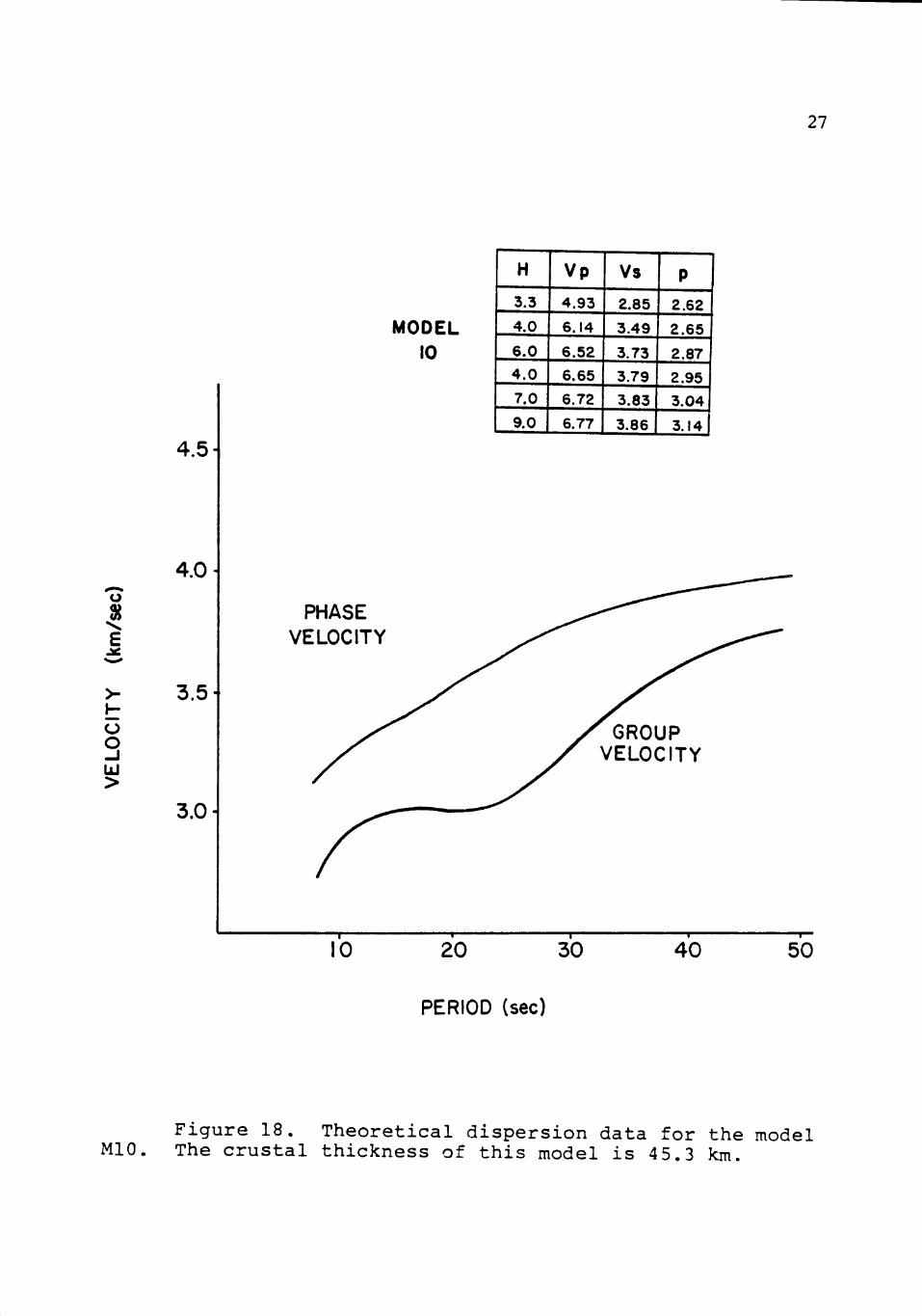
Figure 18. Theoretical dispersion data for the model MlO. The crustal thickness of this model is 45.3 km.

28
MODEL 11
4.5-
4.0-
o
O o -J UJ >
3.5-
3.0-
H
4.3
10.0
6.0
5.0
9.0
12.0
Vp
4.93
6.14
6.52
6.65
6.72
6.77
Vs
2.85
3.49
3.73
3.79
3.83
3.86
P 2.62
2.65
2.87
2.95
3.04
3.14
PHASE VELOCITY
GROUP VELOCITY
10 20 30 40 50
PERIOD (sec)
Figure 19. Theoretical dispersion data for the model Mil. The granitic layer in this model is 5 km. thicker than in the basic model. The crustal thickness is increased to 46.3 km.

29
4.5-
4.0-o
E JiC
>
O o - J UJ >
3.5-
MODEL 12
H 4.3
5.0
6.0
5.0
9.0
12.0
Vp
5.3
6.35
6.75
6.05
7.4
7.57
Vs
3.06
3.62
3.84
3.49
4.21
4.31
P 2.62
2.65
2.87
2.95
3.04
3.14
PHASE VELOCITY
3.0-
GROUP VELOCITY
lo" 20 30 40 50
PERIOD (sec)
Figure 20. Theoretical dispersion data for the model M12. Velocities in all crustal layers are greater than in the basic model.
30
4.5-
4.0-
o (A
E 2C
3.5-
o 3 UJ >
3.0-
MODEL 13
H
4.3
10.0
6.0
5.0
9.0
12.0
Vp 5.3
6.35
6.75
6.05
7.40
7.67
Vs 3.06
3.62
3.84
3.49
4.21
4.31
P 2.62
2.65
2.87
2.95
3.04
3.14
PHASE VELOCITY
GROUP VELOCITY
"l^ 20 30 40 50
PERIOD (sec)
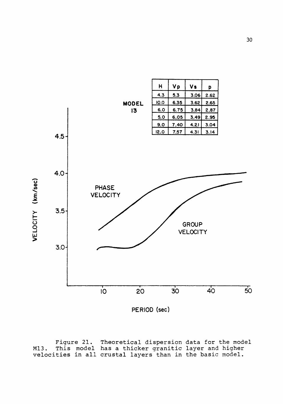
Figure 21. Theoretical dispersion data for the model M13. This model has a thicker granitic layer and higher velocities in all crustal layers than in the basic model.

31
MODEL 14
4.5-
4.0-u
E
o o -J UJ >
H
8.3
5.0
6 .0
5.0
9.0
12.0
Vp
5.3
6.35
6.75
6.05
7.40
7.57
Vs
3.06
3.62
3.84
3.49
4.2J
4.31
P 2.62
2.65
2.87
2.95
3.04
3.14
PHASE VELOCITY
3.5-
3.0-
GROUP VELOCITY
10 20 30 40 50
PERIOD (sec)
Ml 4 Th?c I ^ Jh^^^^tical dispersion data for the model M14. This model has a thicker sedimentary layer and higher velocities in all crustal layers than in the basic model

ear
va
32
trary distance and time references for phase computations.
Particle velocity is computed as a function of frequency by
Fourier inversion of phase information computed from the
phase velocities.
The source function for the synthetic seismograms is
assumed to approximate a step function. This function is
typical of source functions obtained for South American
thquakes (Aki, 1972), and is characterized by a slowly
rying frequency spectrum as observed for earthquake seis
mograms (Goforth, 1976).
Examination of the synthetic seismograms shows that
the character of each seismogram is different. The
theoretical dispersion data reveals that little change in
the phase velocities is caused by variations in the models.
However, marked differences are observed in the group vel
ocity data, particularly for periods less than 20 seconds.
Character change may be interpreted in terms of group vel
ocity variation and, hence, variations in earth structure.
The synthetic seismograms for M3, M4, MlO, and M14
(Figures 3, 6, and 8) exhibit a ringing appearance not so
pronounced in the synthetic for the basic model Ml. The
models have a thicker sedimentary layer (M3, MlO, and M14),
a thicker crust (MlO and M14), or a lower velocity in the
sedimentary layer (M4), than included in the basic model Ml.
The thick sedimentary layer and the low velocity in the

33
sedimentary layer causes the slope of the group velocity
curve to increase for periods less than about 12 seconds.
The increased slope for the group velocity data indicates
strong dispersion for waves with periods less than about
12 seconds. This causes the ringing appearance in the
synthetic seismograms.
The remaining synthetic seismograms exhibit large
increases in the amplitude of wave groups with periods of
about 12 seconds. Relative to the basic model Ml, the
models for which these synthetics are generated have the
following variations: thick basaltic layers (M5 and M6,
illustrated in Figure 4); a thick granitic layer (M2, Mil,
and M13, illustrated in Figures 2, 7, and 8, respectively);
a low velocity layer in the crust (M7, M8, M12, and M13,
illustrated in Figures 5, 7, and 8, respectively); a thin
crust (M9, illustrated in Figure 6); increased velocities
in the crust (M12 and M13, illustrated in Figures 7 and 8).
The amplitude increase is attributed to constructive
interference between wave groups having nearly the same
period and velocity. For M2 and M5 through M9, this inter
ference arises from the increase in the length of the
inverse dispersion branch of the group velocity curve for
periods between about 18 and 10 seconds. For Mil through
M13, the interference is due to the nearly zero slope in
the group velocity curve for periods between about 18 and
10 seconds.

34
The synthetics for M2, Mil, M12, and M13 show the
greatest amplitude increase, indicating that the primary
factors contributing to this change in character are a
thickened granitic layer, increased crustal velocity, and
a low velocity layer. The synthetic for M13 shows that
the amplitude increase is most significant when faster
crustal velocities accentuate the effects of a low velocity
zone.
The amplitude increase in the synthetics at about 12
seconds wave period is similar to the earthquake phase R
(Press and Ewing, 1952). Evidence from the synthetic seis
mograms indicates that the phase R is a phenomenon of ar-
rival of wave groups with periods between 18 and 10 seconds
and nearly the same group velocity. This phenomenon of
near equal group velocity for waves of a range of periods
is due primarily to the effect of the granitic layer in the
crust.
The effect of each portion of the crust on the R^
phase is illustrated by the synthetic seismograms in
Figures 23 and 24 for models containing a thick basaltic
crust only (M15, illustrated in Figure 25), a thin sedi
mentary layer overlaying thick basalt (M16, illustrated in
Figure 26), and a thin granitic layer overlaying thick
basalt (M17, illustrated in Figure 27). Figures 23 and 24
show that the R phase is produced only in the synthetic y
for model M17. The synthetics for models M15 and M16 show
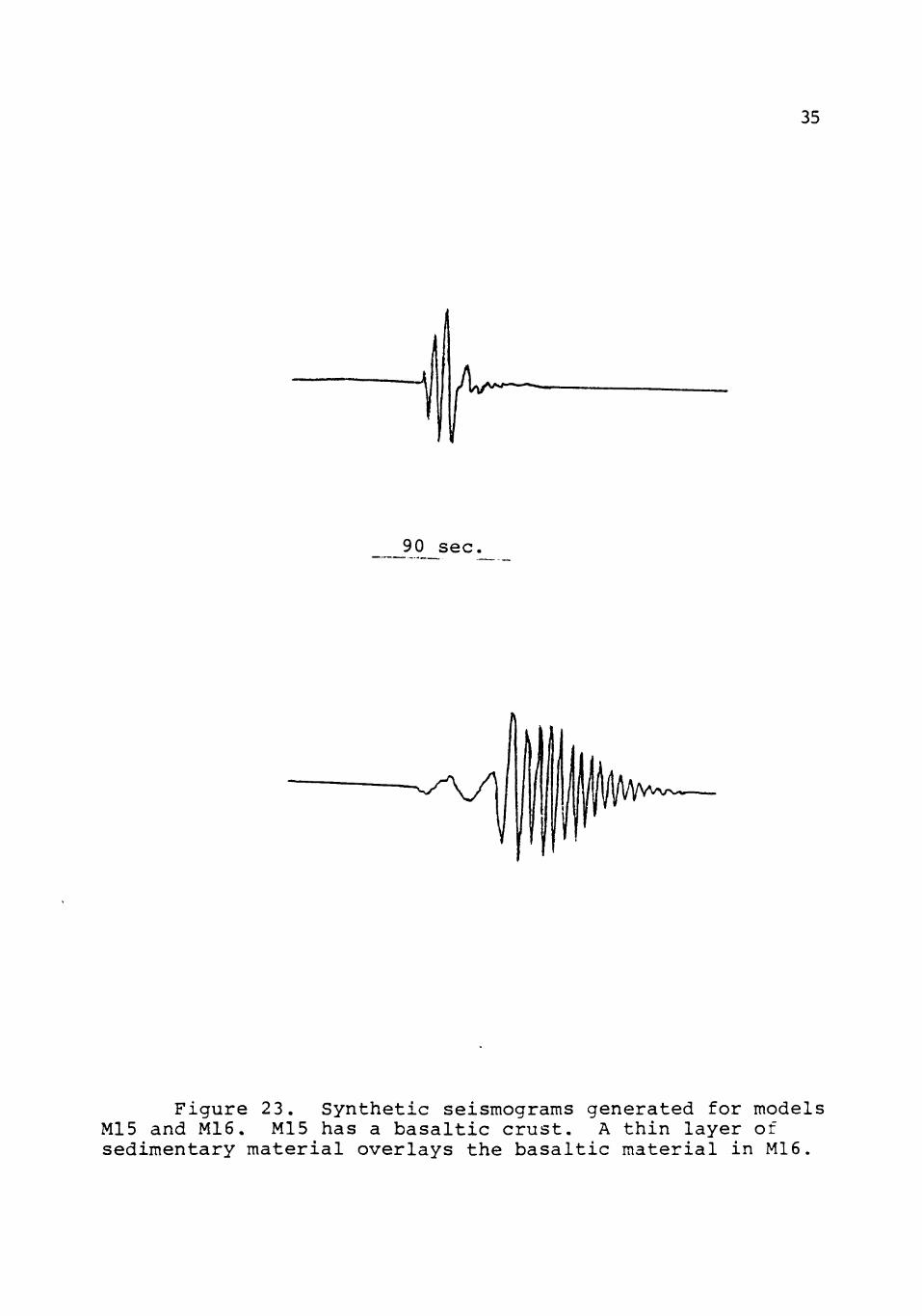
35
90 sec
Figure 23. Synthetic seismograms generated for models M15 and M16. M15 has a basaltic crust. A thin layer of sedimentary material overlays the basaltic material in M16.

36
lyVX/—
90 sec,
Figure 24. Synthetic seismogram generated for model M17. A thin layer of granitic material overlays this basaltic material in the crustal portion of this model.

37
MODEL 15
H
40.0
Vp
7.57
Vs
4.31
P 3.14
4.5-
4.0-
o a> (A
3.5-
3 UJ >
3.0-
PHASE VELOCITY
GROUP VELOCITY
lo" 20 30 40 7o
PERIOD (sec)
Figure 25. Theoretical dispersion data for the model M15. The crustal portion of this model is comprised of a single layer of basaltic material.

38
MODEL 16
H
5.0 35.0
Vp
5.30 7.57
Vs
3.06 4.31
P 2.62
3.14
4.5-
4.0 o (A
3.5-
3 UJ >
3.0-
PHASE VELOCITY
GROUP VELOCITY
10 20 30 40 50
PERIOD (sec)
Figure 26. Theoret ical d ispers ion data for the model M16. The c r u s t a l por t ion of t h i s model i s comprised of a th in layer of sedimentary mater ia l (overlaying a thick b a s a l t i c l aye r . )

39
MODEL 17
H
5.0
35.0
Vp 6.35
7.57
Vs 3.62
4.31
P 2.65
3.14
4.5-
4.0-o <u
PHASE VELOCITY
CJ
O -J UJ >
3.5-
3.0-
ROUP VELOCITY
10 20 30 40 50
PERIOD (sec)
Figure 27. Theoretical dispersion data for the model M17. The crustal portion of this model is comprised of a thin layer of granitic material (overlaying a thick basaltic layer.)

40
only weak dispersion for model M15 and the pronounced ring
ing due to the sedimentary layer in M16.
The synthetic seismograms presented in Figures 2 to 8
and in Figures 23 and 24 clearly illustrate that small
changes in crustal structure cause significant changes in
the characteristics of Rayleigh waves. Increased thickness
of, or decreased velocity in, the sedimentary layer causes
the seismogram to assume a ringing appearance. Thickening
of the granitic layer, the introduction of a low velocity
layer into the crustal model, and increased crustal velo
cities result in amplitude increases in the seismogram re
sembling the earthquake phase R . Identification of these y
characteristics in earthquake seismograms can provide im
portant information about the crustal structure of the
earth.
CHAPTER IV
CORRELATION OF SYNTHETIC SEISMOGRAMS
WITH EARTHQUAKE SEISMOGRAMS
The application of character modeling to the identi
fication of crustal structure requires cross correlation of
synthetic seismograms with earthquake seismograms. When
the earthquake (true) seismograms are reasonably noise free
the correlation may be made visually. However, true seis
mograms are rarely noise free, and numerical cross correla
tion is usually required.
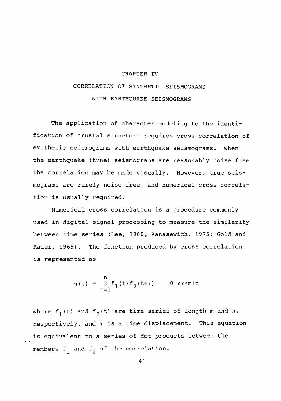
Numerical cross correlation is a procedure commonly
used in digital signal processing to measure the similarity
between time series (Lee, 1960, Kanasewich, 1975: Gold and
Rader, 1969). The function produced by cross correlation
is represented as
n g d ) = Z f (t)f^(t+T) 0 ^T<m+n
t=l ^ ^
where f, (t) and £9^^^ ^"^^ time series of length m and n,
respectively, and x is a time displacement. This equation
is equivalent to a series of dot products between the
members f, and t,. of the correlation.
41

42
The cross correlation function produced from two time
series is a measure of the similarity in frequency content
and the phase difference at each frequency. Time series
which have similar frequency and phase components produce
cross correlation functions which have large maxima and
good symmetry about the maxima.
The Rayleigh waves of two earthquakes with epicenters
in Mexico and off the western coast of Mexico are shown in
Figure 28. Locations of the epicenters are shown in
Figure 29. These Rayleigh waves were recorded at the WWSSN
station in Lubbock, Texas. The travel path between Lubbock
and Event 2 has previously been examined by the author
using Love waves (Crider, 1975), and the crustal model de
rived in that study is the basic model used in the synthe
tic seismogram generation described in Chapter III.
Examination of the earthquake seismograms reveal that
the Rayleigh waves recorded for Event 2 are considerably
different from those recorded for Event 1. The primary
cause for this difference is interference between Rayleigh
wave groups arriving at Lubbock along different azimuths
(e.g. Evernden, 1953). This type of interference is also
expected in Rayleigh waves for Event 1. Visual correlation
between these true seismograms and the synthetic seismo
grams is not possible and numerical cross correlation must
be performed to find any similarity between the true and
synthetic seismograms.

43
—^A
90 sec.
Figure 28. Long period vertical components of seismograms recorded at Lubbock, Texas from two earthquakes along the western coast of Mexico. The locations and times for the earthquakes are: Event 1 (upper) - July 2, 1972, Ooh 34m 42.8^; 6 = 16.4° N; X= 98.5° W. Event 2 (lower) -May 28, 1972, 23^ 11 ^ 36.7S; 9 = 19.3° N; X = 108.3° W.

44
Figure 29. Location of the epicenters for Event 1 and Event 2 and the receiving station. The dashed lines indicate the assumed travel paths between the epicenters and the receiving station. Contours are in fathoms.

45
Numerical cross correlation between the true and syn
thetic seismograms was accomplished on the Sunmark Explor
ation Company's Wang 2200 VP computer. All seismograms
were digitized using a Summagraphics digitizing board inter
faced with the Wang computer. A one-second sample interval
was used in all digitizing.
The cross correlation functions obtained between Event
1 and the suite of synthetic seismograms shown in Chapter
III are illustrated in Figures 30 to 43. The correlation
functions obtained for the models Ml, M9, and MlO, re
presenting different crustal thicknesses, show the crust
between Lubbock and Event 1 to be at least as thick as that
for the basic model Ml. The maximum in the correlation
functions for Ml and the thickened crust model MlO are
much greater than that for the thinned crust model M9.
The maximum of the function for MlO is the greatest,
suggesting that the crustal thickness is somewhat greater
than that for the basic model.
The greatest maximum among all the cross correlation
functions is found in the correlation function for M4 which
corresponds to the same crustal thickness as in Ml but with
a reduced velocity in the sedimentary layer. However, the
poor symmetry observed in the function is indicative of
poor correlation between the seismograms for Event 1 and
M4.
The cross correlation function obtained by comparina

u
46
<D CO
u 0)
cn
o
w u
A4
0) 0 s:
4-1
c 0
•H 4-» U c p
iw
C 0
•H +J to
rH <U U U 0
J->
^ 0
MH
g nJ }H
0 e Ui
•H o; (0
u •H +J <\)
u i : cn cn 0 M u
4J c >. cn
the
o s: m
0) SH
•H I?
3 'C cn (U
•H fa
•P •
rH (0 S
rH (1) iH U d) U TJ 0 0
0 E

47
SI cn j o I
i H CN
s +> iH
c 0) Q) 73 > »
U
0
e 0)
0 x: IW
c 0
•H •P
u c 3
« 4 - l
c 0 •H +J (TJ
i H (U ^ u 0
+J
^ 0
* 4 - l
e fC ^ cn 0 e tn.
•H (U cn u
•H 4J (U
u ^ cn CO 0 u u
•
•P
c > 1
cn (1) x: 4J
.H J : ro
0) }-(
-p •H ^
D 73 D (U
•H fa
V (0
i H 0) ^ U 0 u
48
cn'
o
4J
c • <U ro > S W
i H U (U 0 73
IM
c 0
0 e Q)
•H .C 4J U c p M-(
c 0
•H 4J to
i H
Q) ^ U 0 0
cn cn 0
+J
>H 0
M-l
B (d M CP 0 B cn •H (U cn U
•H JJ (U
u s: u
t
CN ro
(U JH
4J
c > 1
cn (U .c 4-»
:3 73 D Q)
•H fa
4-> (0
i H <U u u 0 u

49
u
cn
o
^ • H S •P rH
c (U <U 'O >
w u
0
e (U
0 x: ^
c 0
• H 4-» U c o
««
c 0
• H +J (0
i H (U J-l
u 0
4J
U 0
MH
e nj
u CP 0
e cn • H 0) cn u
• H +J (U
U JS
cn cn 0 u u
ro ro
<U >H
4J
c > 1
cn Q)
x: 4J
x: •p • H
15 3 73 O (U
• 1 -
fa 4J fd
i H (I) }-l >H 0 o

50
(U
cn o
in
rH S
JJ rH
0) ^3
> o w e >H QJ
ox: C U o o
• H M-t 4J
3 e td }H MH CT
o c o
•H
e cn
•H «d cn
(U u }H -H U -P O Q)
u x: cn c cn > i 0 cn 5H U d)
x:
ro 4J •H
<D 5 5H
D 0) •H 4J fa Id
0)
}H O U

51
cn I
o
yo .H s 4-> r-i C <U > w M
(U T3 0
e (U
0 x: »+-(
c 0
•H 4-> U c 3
^-^
>•* 0
•H +J (d
rH (U }H M 0
•p
u 0
4-4
e (d M tj^ 0
e cn •H (U cn u
•H +J (U
u x: cn cn 0 u u
4J
c > 1
cn 0) x: •p
in ^ ro
(U }H
+j •H >
3 73 tP <U
•r-
fa 4J fd r-\ Q) U U 0 U

52
C 0) 0) 73
> o w e }H 0) o x :
C SH O O
•H MH
U c :3
e fd u o
o -H
e cn
• H 0) (d in
rH (U u J-i -H U 4-> o <u o ^
+J cn c cn >i O m
x: 4->
ro -P •H
Q) ^ U O 73 cn (U
•H 4-) fa fd
rH (U }H >H O U

53
o cn o
00 -H S •P r-^ C 0) <U TJ > 0 W E
U <D
ox: 4-( + j C JH
o o •H U-t -P u c: p
B fd
4 H C7I
o o
•H 4J
cn •H
fd cn r-\ <D u ^ -H o <u u s :
•p cn c cn >i o cn u
x: 4-»
ro x: -p •H
U D TJ cn Q)
•H 4J fa fd
rH <D U u o u

54
t • I
U ; Q)! cn i
(T\
<y» i H s 4J i-i C 0) 0) 73 > W
}-j
0 B 0)
0 x: 4H
c 0
•H -p u c :3
MH
C 0
•H 4J Id
rH <U }H ^ 0
+J
}H 0
UH
e fd >H CP 0 B cn
•H (U cn u
•H +J 0)
u x: cn cn 0 u u
00 ro
dJ }-
4-)
c > l
cn (U x: 4J
x: +j •H ^
3 'd C7 0)
• r
CL 1 -P ( fd
i H (1) }H }H 0 O

55
cn
o
^ S
4J c
rH <u
Q) n3 > fa $H
0
e 0)
0 x: 4H
c 0
•H 4-> U c p
<4H
C 0
•H 4-» fd r-*. Q) U u 0
+J
u 0
MH
e fd u cn 0 e cn
•H 0) cn u
•H +J (U
0 x: cn cn 0 u u
+J c > i
cn 0) £ j j
cr> jC ro
(U 5H
+J •H 5
P 73 cr 0)
•H fa
JJ fd
rH 0) M M 0 u

56
o cn o
+J c Q) > W
u
i H (U Ti 0 E Q)
0 J: yu
G 0
•H 4-> U C P
4H
C 0
•H JJ fd
rH (U U u 0
4J
}H 0
t+H
E Id k CP 0 E cn
•H
<u cn
u •H 4J 0)
U £
cn cn 0 u u
+J c > 1
cn (U x: 4-!
ox: ^
0) ^
4J •H >
P 'C c: o
•H fa
4J Id
f-i <D U U 0 u
57
CN
U
cn
o CJ^
4J r-\ C QJ > H
»H
QJ 73 0 E QJ
0 x: MH
c 0
•H +J u c p
4H
c 0
•H 4-J fd r-\ <u u u 0
-P
U 0
«4H
E fd i j D 0 E cn
•H Q) cn u
•H ^ QJ
u x: cn cn 0 u u
4J C > i
cn QJ
£ 4J
rH ^ ^
QJ U
• P • H
15 P TS cn QJ
•H fa
4J fd
rH QJ U U 0 ^

58
ro
u QJ cn
o ,
•P >H C QJ QJ T l > fa U
0 E QJ
0 x: 4H
<-• 0
•H •P U C P
4-1
C 0
•H 4J fd
PH QJ »H ^ 0
+J
^ 0
4H
E .•0 u cn 0 E cn
• H QJ cn u
• H +J QJ
u x: cn cn 0 u u
•p c >t CO
QJ x: 4-»
<N x : "^
Q) 1
4-1 • H
^
P T5 CP QJ
•H fa
4-> fd
l-i QJ 4
U 0 u
59
u QJ
cn o
I-H
• • ^
t-i
S •p >-{
c QJ QJ TJ > fa
U
0 E QJ
0 x: 4H
C 0
•H 4J U C P
4H
c 0 •H 4J fd
r-i QJ }H ^ 0
-P
U 0
m
E (d M cn 0 E cn
•H QJ cn
U •H 4J QJ
0 x:
cn cn 0 u u
ro ^
QJ U
4J
c > 1
cn
QJ x: 4J
£ 4-) •H ^
P 73 Cn QJ
•H fa
•p Id
rH QJ V u 0 u

60
Event 1 and the models M2 and M7 exhibit large amplitudes
and good symmetry indicating good correlation. These cor
relation functions'suggest that the crust between Lubbock
and the Event 1 epicenter contains either a low velocity
layer or a thicker granitic layer than included in the basic
model Ml. The larger amplitude of the M2 cross correlation
suggests that a thicker granitic layer is the more likely
of the two alternatives.
Models Mil and M13 contain granitic layers thicker
than that in the basic model Ml. However, the crustal vel
ocity structure in these two models is significantly dif
ferent from that of the basic model Ml. The nearly zero
correlations for these models demonstrate the failure of
these models to describe the crustal structure between
Lubbock and the Event 1 epicenter.
The cross correlation functions obtained between Event
2 and the suite of synthetic seismograms are shown in
Figures 44 to 57. Large maxima are observed in the cross
correlation functions for models M2, M3, M4, M7, and MlO
and the Event 2 Rayleigh waves (Figures 45, 46, 47, 50, and
53, respectively). The greatest maximum among these cor
relation functions is observed in the function for the
thickened crust model, MlO, suggesting that the thickness of
the crust between Lubbock and Event 2 is greater than that
included in Ml. However, this function lacks the symmetry
expected of good correlation.

61
o '• QJ
cn
o
CM
4J U
QJ cn > Id W Xi
u QJ
o x: 4H 4J
C }H
o o •H 4H 4J U E c Id p u
4H CP o o
•H 4J
E cn
• H QJ
fd cn rH QJ U ». -H J-1 4J O QJ
JJ
cn
cn cn O u U QJ
X 4J
^' X 'd' -P
•H QJ ^ >-i P 73 cn QJ
•H 4-1 fa fd
QJ r-{ U Q) U 73 O O U E
62
u QJ
cn
o
CN CN S
4J r-< C QJ QJ 73 > O W E
}H QJ ox 4H 4->
C }H O O
• H 4H 4->
p
c (d }H
4H cn o
c o
• H 4J
E cn
• H QJ
fd cn r-\ QJ u }H -H U V O QJ O X
4-» cn c cn >i O cn >H U QJ
X 4J
• in X •^ 4->
•H QJ ^ JH P T5 CP QJ
•H 4J fa fd
QJ U U O U
63
u QJ
cn
o
CN ro S
4-> ^ C QJ QJ T i > fa U
0 E QJ
0 X 4H
c 0
• H •p
u c p
4H
C 0
• H P fd
t-\
QJ }H ^ 0
4J
^ 0
4H
E fd u cn o E cn
•H QJ cn u
- H 4J QJ
U X
cn cn 0 u u
VO '3 '
QJ U
4-> c > 1
cn QJ X 4-1
X 4J •H ^
P TJ cn QJ
•H
fa 4J Id
rH QJ U U 0 U

64
ul Q J i cn o! o i
' CN
«:r S
4J r-\
c QJ QJ T3 > fa U
0 £ QJ
0 X 4H
c 0
•H 4-1 U c p
4H
c 0
•H 4-J fd
i H QJ U U 0
+J
SH 0
4-1
E fd u CP 0 E cn
•H QJ cn u
•H 4J QJ
0 X
cn cn 0 u u
r ^
QJ u
4J c > l
cn QJ X •p
X 4-1 •H ?
P 73 cn QJ
•H fa
4-1 fd
rH QJ JH JH 0 U

65
in CN X
4J r-i C QJ Q) 73 > O W E
J H QJ O X
4 H 4->
c u o o
•H 4H 4J U
p
E fd u
4H CP
o
O I QJ
cn
o
o • H 4J
E cn
• H QJ
fd tn H QJ U JH - H JH 4J O QJ O X
4J cn C cn >i O tn JH U GJ
X 4->
• 00 X -a * 4->
• H QJ ^ JH p T3 cn d)
•H +J fa Id
r-{ QJ J H J H O U

66
o QJ
cn
o
VO CN 2
4J r^ C QJ QJ TJ > O W E
JH O
4H
QJ X
C JH
o o •H 4H 4-> U
p
E fd JH
4H CP O
o •H 4J
E cn H QJ
fd tn i H QJ o JH - H JH 4J O QJ U X
4J cn C cn > i O tn JH U QJ
X 4J
• <j\ X r r 4->
•H QJ > JH p 73 CP QJ
•H 4J fa Id
r-i QJ JH JH O U

67
cn!
O !
CN
4-)
c QJ QJ 7 3 > O fa E JH O
4H
QJ X 4J
J : JH o o •H 4H 4J u c p
E Id JH
4H CP O
c o
•H 4J
E cn
• H QJ
fd tn rH QJ u JH - H V4 4J O QJ U X
4J tn c cn > i O cn JH CJ QJ
X 4->
O X in 4J
•H QJ 5 JH p 73 cn QJ
•H 4-1 fa Id
rH QJ JH U o o

68
u QJ cn o as
CO CN S
4J r^
c QJ QJ 73 > fa JH
0 E QJ
0 X 4H
c 0
•H 4-> U G P
4H
C 0
•H 4-> Id
r-^ QJ JH JH 0
4J
JH 0
4H
E Id JH CP 0 E cn
•H QJ cn U
•H 4-> d)
U X
cn cn 0 JH
u
p c >^ cn QJ
X 4->
r^ X i n
QJ U
4J •H 5
P 73 cn QJ
• r
fa 4J Id
rH QJ JH JH 0 U

69
o Q) CO
o
CN S
4J <H C OJ QJ 73 > O
w s }H QJ O Xi
UH +J
o o •H 4H •P U
p E (d JH
4H C7> O
O B tn
•H
fd to rH QJ U JH - H JH 4J O QJ U ^
in C in >i 0 in JH U QJ
x: 4J
• CN xi in 4J
•H QJ ^ JH P TJ CT» QJ
•H 4-» fa Id
rH QJ U U O U

70
CN S
4-> C
rH QJ
QJ 73 > fa U
0 E QJ
0 X 4H
c 0
•H 4J U C P
4H
C 0
•H 4J fd
r-i OJ JH JH 0
4J
U 0
4-1
E fd V4 cn 0 E cn
•H QJ cn U
•H 4J QJ
U X
cn cn 0 u u
ro i n
Q) U
4J
c >, cn QJ X •p
X 4-» •H ?
P T3 CP QJ
•H fa
+J Id
rH QJ U U 0 u

71
CN S
QJ! cn
o as
4J C QJ QJ TJ > O W E
O 4H
QJ X 4J
o o •H 4-1
U E c Id P V4
4H CP
o o
•H 4-)
E cn
• H QJ
fd cn rH QJ u JH -H JH +J O QJ U X
P cn c cn >i O cn JH U QJ
X 4->
^* X in 4->
•H QJ ^ JH P 'O cn QJ
•H 4J fa Id
rH QJ u JH O U

CN
CN S
72
u: QJi cn;
i o as
4J rH
c QJ QJ 73 > W
JH
0 E
QJ 0 X
4H
C 0
•H 4J U C P
4H
C 0
•H 4-1 fd
r-i d) U U 0
4J
U 0
4H
E fd ^ cn 0 E cn
•H QJ cn
u •H 4J QJ
U X
cn cn 0 JH U
4-1
c > 1
cn QJ
X 4-1
m X in
d) u
4-1 •H >
P T3 cn QJ
•H fa
4-1 fd
l-i d) u u 0 u

73
ro
CN S
u: d)
oi CTtl
4J C
t-i QJ
QJ T) > fa U
0 E QJ
0 X 4H
C 0
•H V U
c p
IW
c 0 •H 4J fd
rH QJ JH U 0
4-1
JH 0
4H
E fd 1
cn 0 E cn
•H QJ cn
u •H 4J QJ
U X
cn cn 0 JH U
4-1
c > 1
cn QJ
X 4-1
VO X in
QJ JH
4J •H ^
P 73 cn QJ
•H fa
4J fd
r-i QJ JH JH 0 U

74
CN S
U QJ cn
o as
•P r^
c QJ QJ 73 > fa U
0 E QJ
0 X 4H
c 0
•H +J U c p
4H
C 0
• H 4-1 fd r^ d) u u 0
4J
JH 0
4H
E fd JH Cn 0 E cn
•H QJ cn u
•H 4J QJ
U X
cn cn 0 u u
r in
QJ u
4J C > i
cn QJ
X 4-1
X 4-1 •H ^
P 73 CP QJ
•H fa
4-1 fd
rH QJ JH U 0 U
75
Symmetry and large amplitude are observed in the
cross correlation function for the basic model Ml (Figure
39) and the Event 2 Rayleigh waves. It should be noted
that the maximum of the correlation function for the model
Ml is nearly as large as that in the MlO correlation. This
indicates that the correct model for the crustal structure
between Lubbock and the Event 2 epicenter is probably only
slightly different from the model Ml. The large amplitude
observed in the M2, M3, M4, and M7 correlation functions
suggest that the model should include a thicker granitic or
sedimentary layer than included in the model Ml, in addi
tion to a crustal low velocity layer.
Cross correlation of the suite of synthetic seismo
grams with Rayleigh waves from two earthquakes in Mexico
shows that the crustal structures between the epicenters
for the two events and Lubbock are similar. These struc
tures are slightly different from that determined using
Love waves from Event 2 in that they probably have thicker
granitic and sedimentary layers than included in the basic
model Ml in addition to a low velocity layer in the crust.

CHAPTER V
CONCLUSIONS
1. Synthetic seismograms that reveal the character
of seismic waves in a given layered earth model may be gen
erated from theoretical phase velocities for the model.
2. The earthquake phase R may be explained as the g
result of waves with periods between 18 and 10 seconds
having nearly the same group velocity due to the presence
of the granitic layer in the crust.
3. Cross correlation of synthetic seismograms for
several earth models with true earthquake seismograms
verify that the crust beneath Northern Mexico is 41.3 km.
thick and is comprised of a slow velocity, 4.3 km. thick
sedimentary layer, a 5.0 km. thick granitic layer, a
crustal low velocity layer, and 32 km. of basaltic material
4. Visual or numerical correlation of synthetic
seismograms for varying earth models with earthquake
seismograms may give a direct determination or a verifi
cation of an earth model.
76

CHAPTER VI
RECOMMENDATIONS
The results of this study have been limited to the
explanation of the characteristics of seismograms of earth
quake Rayleigh waves having periods greater than about 9
seconds. However, true seismograms record Rayleigh waves
and other surface waves with shorter periods as well.
These shorter periods may have pronounced effects on the
characteristics of the seismograms. For this reason the
following recommendations for further study are made.
1) Extend the range of wave periods included in
the synthetic seismogram to include periods
at least as low as 5 seconds. The inclusion
of these short wave periods may provide useful
data on the propagation of microseisms in the
period range of 5-6 seconds.
2) Include higher mode Rayleigh waves in the con
struction of the synthetic seismograms. In
clusion of these high velocity, short period
waves may provide clarification for the
77
^fWB^W
78
characteristics of the early portions of
earthquake Rayleigh wave seismograms which have
not been investigated in this study.
LIST OF REFERENCES
Aki, K., 1960. Study of Earthquake Mechanism by a Method of Phase Equalization Applied to Rayleigh and Love Waves, Journal of Geophysical Research, 65, p. 729-7T0: ~ ~
1972. "Earthquake Mechanism." In: A. R. Ritsema (Editor), The Upper Mantle. Tectonophysics, 13 p. 423-446:
Alterman, Z., Jarosch, H., and Pekeris, C. L., 1959. Oscillations of the Earth, Proceedings of the Royal Astronomical Society of London, A, 252, p. 80-95.
Bloch, L., Hales, A. L., and Landisman, M., 1969. Velocities in the Crust and Upper Mantle of Southern Africa from Multi-Mode Surface-Wave Dispersion, Bulletin of the Seismological Society of America, 59, p. 1599-1630.
Braile, L. W. , and Keller, G. R. , 1975. Fine Structure of the Crust Inferred from Linear Inversion of Rayleigh-Wave Dispersion, Bulletin of the Seismological Society of America, 65, p. 71-83.
Brune, J. N., Nafe, J. E., and Oliver, J. E., 1960. A Simplified Method for the Analysis and Synthesis of Dispersed Wave Trains, Journal of Geophysical Research, 65, p. 287-303.
Brune, James, and Dorman, J., 1963. Seismic Waves and Earth Structure in the Canadian Shield, Bulletin of the Seismological Society of America, 43, p. 167-210.
Bullen, K. E., 1965. An IntrocSuction to the Theory of Seismology, Cambridge University Press.
Crider, R. L., 1975. Structure of the Crust and Upper Mantle Beneath Mexico from Love Wave Dispersion, Unpublished Manuscript, Texas Tech University.
79

80
Dorman, J., Ewing, M., and Oliver, J., 1960. Study of Shear-Velocity Distribution in the Upper Mantle by Mantle Rayleigh Waves, Bulletin of the Seismological Society of America, 50, p. 87-115.
Dorman, J. , and Ewing, M., 1962. Numerical Inversion of Seismic Surface Wave Dispersion Data and Crust-Mantle Structure in the New York-Pennsylvania Area, Journal of Geophysical Research, 67, p. 5227-5241.
Evernden, J. F., 1953. Direction of Approach of Rayleigh Waves and Related Problems, Bulletin of the Seismological Society of America, 43, p. 335-374.
Goforth, Tom T. , 1976. A Model Study of the Effect on the Rayleigh Spectrum of Lateral Heterogeneity in Earthquake Source Regions, Journal of Geophysical Research, 81, p. 3599-3606.
Gold, B., and Rader, C. M., 1969. Digital Processing of Signals, McGraw-Hill Book Company.
Haskell, N. A., 1953. Dispersion of Surface Waves on Multi-layered Media, Bulletin of the Seismological Society of America, 43, p. 17-43.
Kanasewich, E. R. , 1975. Time Sequence Analysis in Geophysics, The University of Alberta Press, Edmonton, Alberta, Canada.
Lee, Y. W., 1960. Statistical Theory of Communication, John Wiley and Sons, Inc., New York, New York.
Marion, J. B., 1967. Classical Dynamics, Academic Press, New York, New York.
McEvilly, T. v., 1964. Central U. S. Crust-Upper Mantle Structure from Love and Rayleigh Wave Phase Velocity Inversion, Bulletin of the Seismological Society of America, 54, p. 1997-2015.
Press, Frank, and Ewing, Maurice, 1952. Two Slow Surface Waves Across North America, Bulletin of the Seismological Society of America, 42, p. 219-228.
Richter, C. F., 1958. Elementary Seismology, W. H. Freeman and Company, Inc., San Francisco, California.
Sato, Y., 1960. Synthesis of Dispersed Surface Waves by Means of Fourier Transform, Bulletin of the Seismological Society of America, 50, p. 417-426.