Additive Models and Trees

Lecture Notes for CMPUT 466/551

Nilanjan Ray

Principal Source: Department of Statistics, CMU

Topics to cover

• GAM: Generalized Additive Models

• CART: Classification and Regression Trees

• MARS: Multiple Adaptive Regression Splines

Generalized Additive Models

What is GAM?

)()()(),,,|( 221121 ppp XfXfXfXXXYE

Compare GAM with Linear Basis Expansions (Ch. 5 of [HTF])Similarities? Dissimilarities?

Any similarity (in principle) with Naïve Bayes model?

The functions fj are smoothing functions in general, such as splines, kernelfunctions, linear functions, and so on…

Each function could be different, e.g., f1 can be linear, f2 can be a naturalspline, etc.

Smoothing Functions in GAM

• Non-parametric functions (linear smoother)– Smoothing splines (Basis expansion)– Simple k-nearest neighbor (raw moving average)– Locally weighted average by using kernel weighting– Local linear regression, local polynomial regression

• Linear functions• Functions of more than one variables

(interaction term)

• Example:

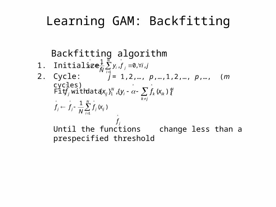
Learning GAM: Backfitting

Backfitting algorithm1. Initialize:

2. Cycle: j = 1,2,…, p,…,1,2,…, p,…, (m cycles)

Until the functions change less than a prespecified threshold

jifyN j

N

ii ,,0,

1

1

Nik

jkki

Nijj xfyxf 11 )}({,}{datawithFit

)(1

1ij

N

ijjj xf

Nff

jf

Backfitting: Points to Ponder

),0(~,)( 2

1

NXfYp

jjj

)()|)(( jjjk

jkk XfXXfYE

Computational Advantage?

Convergence?

How to choose fitting functions?

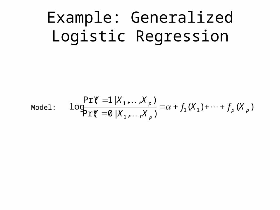
Example: Generalized Logistic Regression

Model: )()(),,|0Pr(

),,|1Pr(log 11

1

1pp

p

p XfXfXXY

XXY

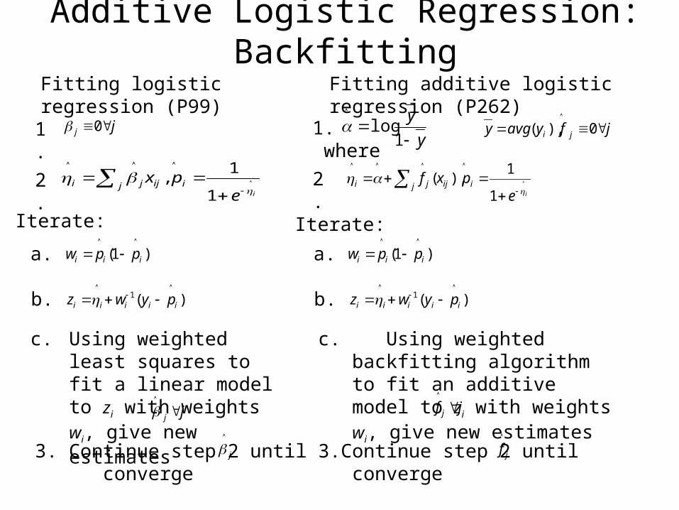
Fitting logistic regression (P99) Fitting additive logistic regression (P262)

1. jj

0

2.

iepx iijj ji

1

1,

Iterate:

)1(

iii ppw

)(1

iiiii pywz

Using weighted least squares to fit a linear model to zi with weights wi, give new estimates jj

3. Continue step 2 until converge

j

1. where y

y

1log jfyavgy ji

0),(

2.

iepxf iijj ji

1

1),(

Iterate:

b.

a. a.

c. c. Using weighted backfitting algorithm to fit an additive model to zi with weights wi, give new estimates

b.

jf j

3.Continue step 2 until converge

)1(

iii ppw

)(1

iiiii pywz

jf

Additive Logistic Regression: Backfitting

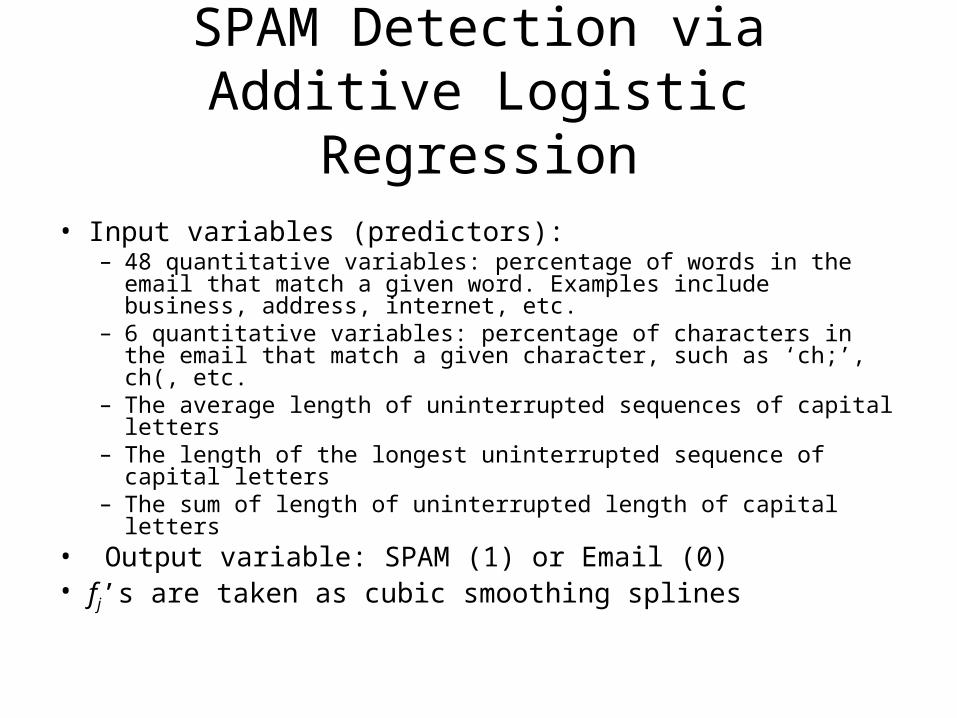
SPAM Detection via Additive Logistic Regression

• Input variables (predictors):– 48 quantitative variables: percentage of words in the email that

match a given word. Examples include business, address, internet, etc.

– 6 quantitative variables: percentage of characters in the email that match a given character, such as ‘ch;’, ch(, etc.

– The average length of uninterrupted sequences of capital letters– The length of the longest uninterrupted sequence of capital

letters– The sum of length of uninterrupted length of capital letters

• Output variable: SPAM (1) or Email (0)• fj’s are taken as cubic smoothing splines

SPAM Detection: Results

True Class Predicted Class

Email (0) SPAM (1)

Email (0) 58.5% 2.5%

SPAM (1) 2.7% 36.2%

93.07.22.36

2.36

Sensitivity: Probability of predicting spam given true state is spam =

Specificity: Probability of predicting email given true state is email = 96.05.25.58

5.58

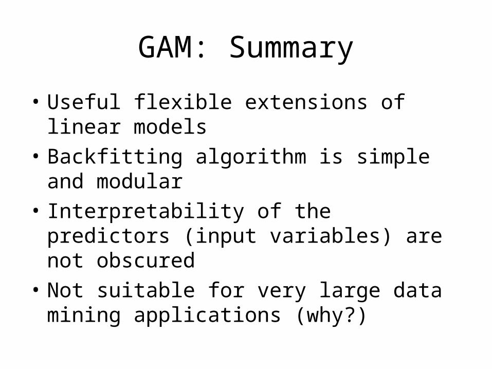
GAM: Summary

• Useful flexible extensions of linear models

• Backfitting algorithm is simple and modular

• Interpretability of the predictors (input variables) are not obscured

• Not suitable for very large data mining applications (why?)

CART

• Overview– Principle behind: Divide and conquer– Partition the feature space into a set of rectangles

• For simplicity, use recursive binary partition

– Fit a simple model (e.g. constant) for each rectangle

– Classification and Regression Trees (CART)• Regress Trees• Classification Trees

– Popular in medical applications

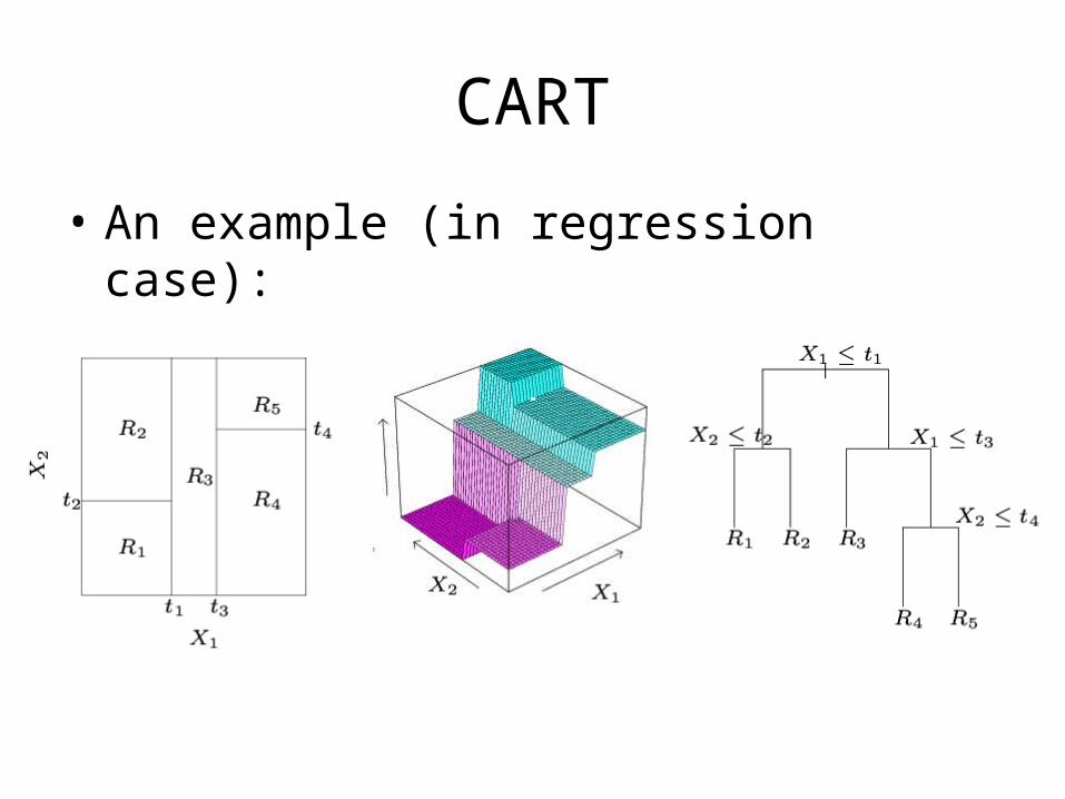
CART

• An example (in regression case):

Basic Issues in Tree-based Methods

• How to grow a tree?

• How large should we grow the tree?

Regression Trees

• Partition the space into M regions: R1, R2, …, RM.

)|(,

)()(1

miim

M

mmm

Rxyaveragecwhere

RxIcxf

Note that this is still an additive model

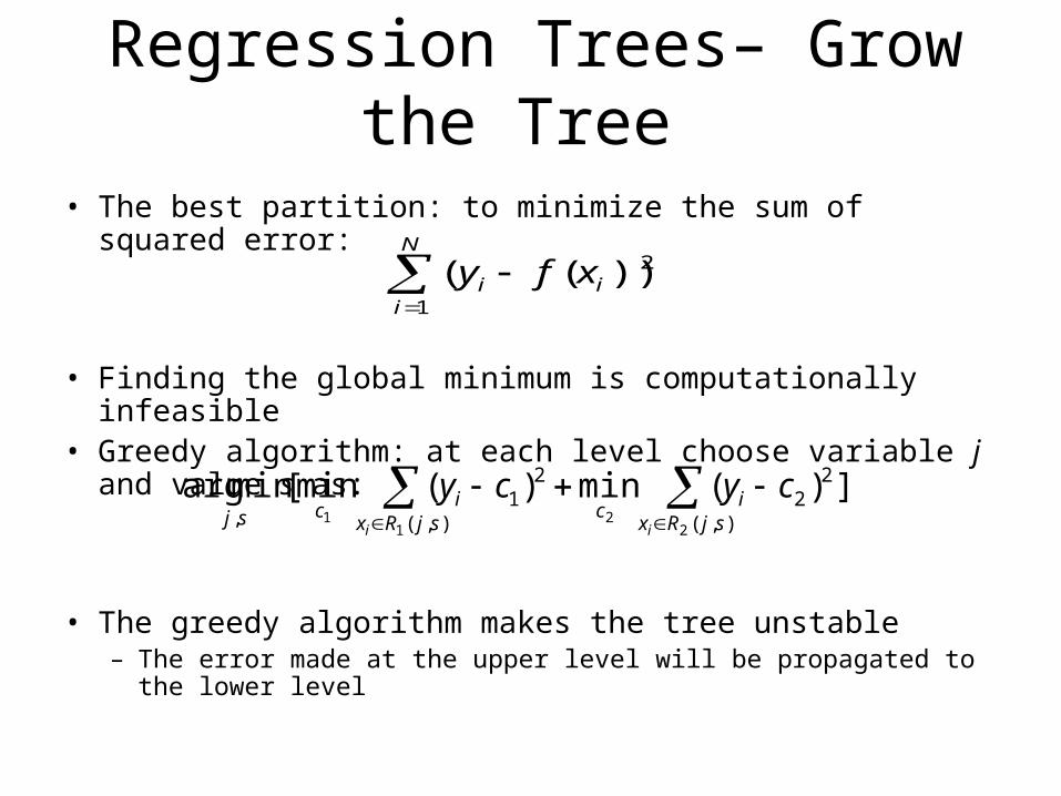
Regression Trees– Grow the Tree

• The best partition: to minimize the sum of squared error:

• Finding the global minimum is computationally infeasible• Greedy algorithm: at each level choose variable j and

value s as:

• The greedy algorithm makes the tree unstable– The error made at the upper level will be propagated to the lower

level

N

iii xfy

1

2))((

])(min)(min[minarg),(

22

),(

21

,2

21

1

sjRxi

csjRxi

csjii

cycy

Regression Tree – how large should we grow the tree ?

• Trade-off between bias and variance– Very large tree: overfit (low bias, high variance)– Small tree (low variance, high bias): might not

capture the structure

• Strategies:– 1: split only when we can decrease the error

(usually short-sighted)– 2: Cost-complexity pruning (preferred)

Regression Tree - Pruning

• Cost-complexity pruning:– Pruning: collapsing some internal nodes– Cost complexity:

– Choose best alpha: weakest link pruning (p.270, [HTF])

• Each time collapse an internal node which add smallest error• Choose from this tree sequence the best one by cross-

validation

||)()(||

1

TTQNTCT

mmm

Penalty on the complexity/size of the tree

Cost: sum of squared errors

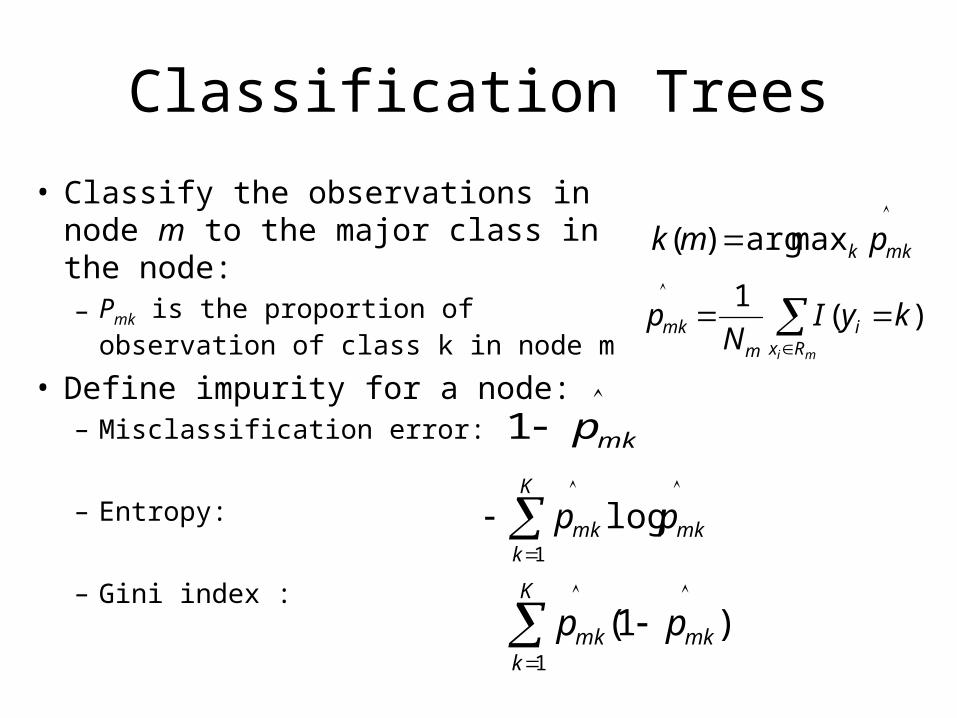
Classification Trees

• Classify the observations in node m to the major class in the node:– Pmk is the proportion of observation

of class k in node m

• Define impurity for a node:– Misclassification error:

– Entropy:

– Gini index : )1(1

mk

K

kmk pp

mkk pmk maxarg)(

mkp1

mk

K

kmk pp

1

log

mi Rx

im

mk kyIN

p )(1

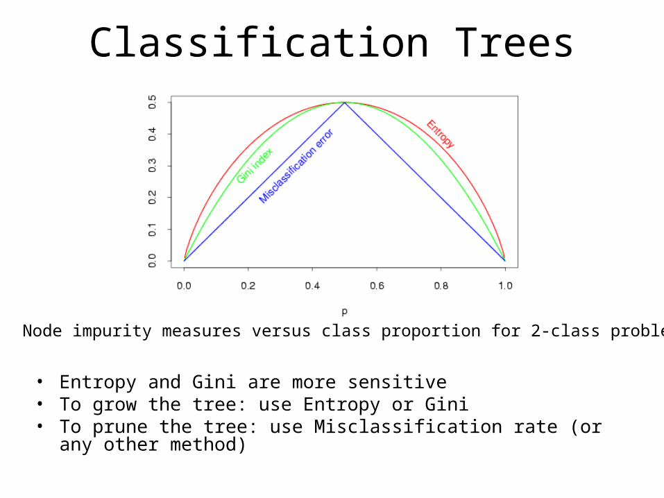
Classification Trees

• Entropy and Gini are more sensitive• To grow the tree: use Entropy or Gini• To prune the tree: use Misclassification rate (or any other method)

Node impurity measures versus class proportion for 2-class problem

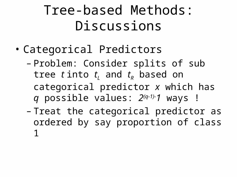
Tree-based Methods: Discussions

• Categorical Predictors– Problem: Consider splits of sub tree t into tL

and tR based on categorical predictor x which has q possible values: 2(q-1)-1 ways !

– Treat the categorical predictor as ordered by say proportion of class 1

Tree-based Methods: Discussions

• Linear Combination Splits– Split the node based on– Improve the predictive power– Hurt interpretability

• Instability of Trees– Inherited from the hierarchical nature– Bagging (section 8.7 of [HTF]) can reduce the

variance

sXa jj

Bootstrap Trees

Construct B number of trees from B bootstrap samples– bootstrap trees

Bootstrap Trees

Bagging The Bootstrap Trees

B

b

bbag xf

Bxf

1

* )(ˆ1)(ˆ

)(ˆ * xf b is computed from the bth bootstrap sample

in this case a tree

Bagging reduces the variance of the original tree by aggregation

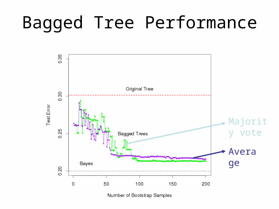
Bagged Tree Performance

Majority vote

Average

MARS

• In multi-dimensional spline the basis functions grow exponentially– curse of dimensionality

• A partial remedy is a greedy forward search algorithm– Create a simple basis-construction dictionary– Construct basis functions on-the-fly– Choose the best-fit basis function at each step

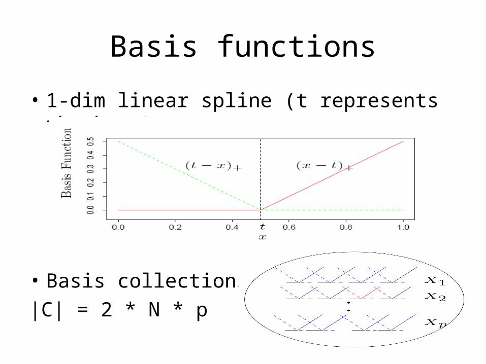
Basis functions

• 1-dim linear spline (t represents the knot)

• Basis collections C:

|C| = 2 * N * p

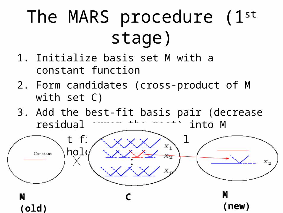
The MARS procedure (1st stage)

1. Initialize basis set M with a constant function

2. Form candidates (cross-product of M with set C)

3. Add the best-fit basis pair (decrease residual error the most) into M

4. Repeat from step 2 (until e.g. |M| >= threshold)

M (old) C M (new)

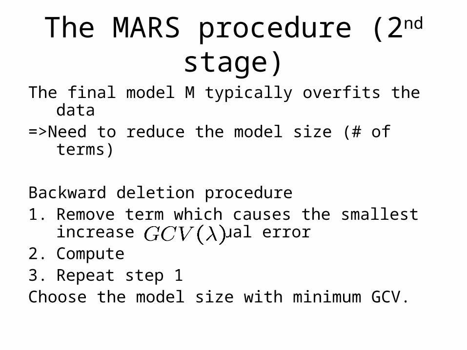
The MARS procedure (2nd stage)

The final model M typically overfits the data=>Need to reduce the model size (# of terms)

Backward deletion procedure1. Remove term which causes the smallest

increase in residual error2. Compute3. Repeat step 1Choose the model size with minimum GCV.

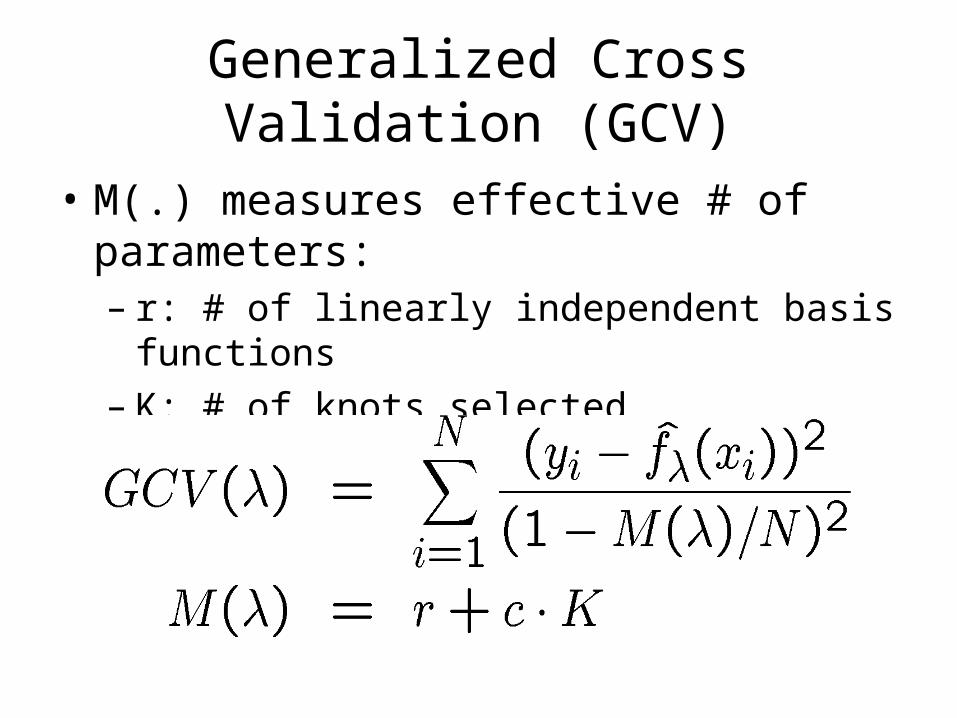
Generalized Cross Validation (GCV)

• M(.) measures effective # of parameters:– r: # of linearly independent basis functions– K: # of knots selected– c = 3

Discussion

• Piecewise linear reflected basis– Allow operation on local region– Fitting N reflected basis pairs takes O(N)

instead of O(N^2)• Left-part is zero, right-part differs by a constant

X[i] X[i+1]

X[i-1] X[i+2]

Discussion (continue)

• Hierarchical model (reduce search computation)– High-order term exists => some lower-order

“footprints” exist• Restriction: Each input appear at most once in a

product:e.g. (Xj - t1) * (Xj - t1) is not considered

• Set upper limit on order of interaction– Upper limit of 1 => additive model

• MARS for classification– Use multi-response Y (N*K indicator matrix)– Masking problem may occur– Better solution: “optimal scoring” (Chapter 12.5 of

[HTF])

MARS & CART relationship

IF

• replace piecewise linear basis by step functions

• keep only the newly formed product terms in M (leaf nodes of a binary tree)

THENMARS forward procedure

= CART tree growing procedure