Kernel Methods

Lecture Notes for CMPUT 466/551

Nilanjan Ray

Kernel Methods: Key Points• Essentially a local regression (function estimation/fitting) technique

• Only the observations (training set) close to the query point are considered for regression computation

• While regressing, an observation point gets a weight that decreases as its distance from the query point increases

• The resulting regression function is smooth

• All these features of this regression are made possible by a function called kernel

• Requires very little training (i.e., not many parameters to compute offline from the training set, not much offline computation needed)

• This kind of regression is known as memory based technique as it requires entire training set to be available while regressing

One-Dimensional Kernel Smoothers

• We have seen that k-nearest neighbor directly estimates Pr(Y|X=x)

• k-nn assigns equal weight to all points in neighborhood

• The average curve is bumpy and discontinuous

• Rather than give equal weight, assign weights that decrease smoothly with distance from the target points

xNxyAvexf kii |ˆ

Nadaraya-Watson Kernel-weighted Average

• N-W kernel weighted average:

• K is a kernel function:

N

i i

N

i ii

xxK

yxxKxf

1 0

1 00

,

,ˆ

0

00 ,

xh

xxDxxK

0 and 0 ,1 ,0

such that Kfunction smooth Any 2 dxxKxdxxxKdxxKxK

where

Typically K is also symmetric about 0

Some Points About Kernels

• hλ(x0) is a width function also dependent on λ• For the N-W kernel average hλ(x0) = λ• For k-nn average hλ(x0) = |x0-x[k]|, where x[k] is the

kth closest xi to x0

• λ determines the width of local neighborhood and degree of smoothness

• λ also controls the tradeoff between bias and variance– Larger λ makes lower variance but higher bias (Why?)

• λ is computed from training data (how?)

Example Kernel functions

• Epanechnikov quadratic kernel (used in N-W method)

• tri-cube kernel

• Gaussian kernel

{

;1 t if 14

3

otherwise. 0

00

2

,

ttD

xxDxxK

{

;1 t if 1

otherwise. 0

00

33

,

ttD

xxDxxK

)2

)(exp(

2

1,

2

20

0 xx

xxK

Compact – vanishes beyond a finite range (such as Epanechnikov, tri-cube)Everywhere differentiable (Gaussian, tri-cube)

Kernelcharacteristics

Local Linear Regression

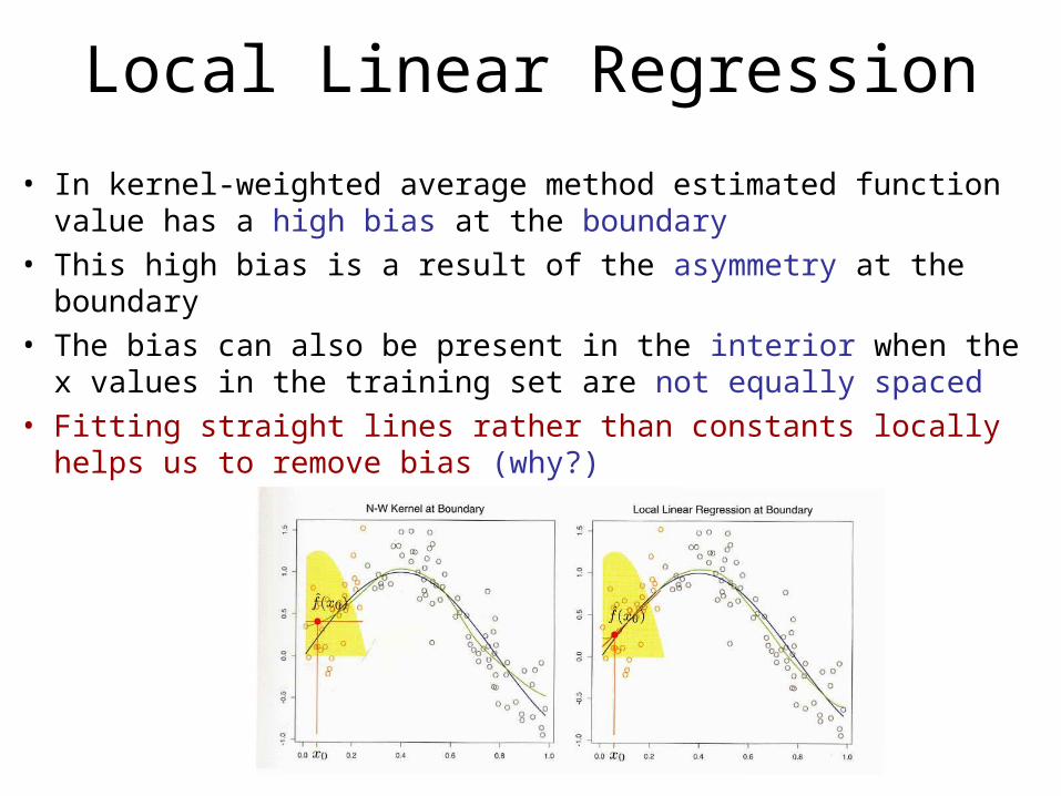
• In kernel-weighted average method estimated function value has a high bias at the boundary

• This high bias is a result of the asymmetry at the boundary• The bias can also be present in the interior when the x values

in the training set are not equally spaced• Fitting straight lines rather than constants locally helps us to

remove bias (why?)

Locally Weighted Linear Regression

• Least squares solution:

• Note that the estimate is linear in yi• The weights li(xi) are sometimes referred to as

the equivalent kernel

ii

T

N

iii

TTT

N

iiii

xx

xxKithxWNN

xbithBN

,xxb

yxl

yxWBBxWBxbxxxxf

xxxyxxK

,element diagonal with matrix diagonal

row with matrix regression 2

1 :function valued-vector

ˆˆˆ

,min

00

T

10

0

1

000000

2

1000

, 00

Ex.

Bias Reduction In Local Linear Regression

• Local linear regression automatically modifies the kernel to correct the bias exactly to the first order

0 and 1 :since

ˆ

ˆ

100

10

10

20000

10

2000

10

200

1000

100

100

N

iii

N

ii

N

iii

N

iii

N

iii

N

iii

N

ii

N

iii

xlxxxl

RxlxxxfxfxfEbias

Rxlxxxfxf

Rxlxxxfxlxxxfxlxf

xfxlxfE Write a Taylor series expansion of f(xi)

Ex. 6.2 in [HTF]

Local Polynomial Regression• Why have a polynomial for the local fit? What would be

the rationale?

• We will gain on bias; however we will pay the price in terms of variance (why?)

ii

dT

N

iii

TTTd

j

jj

N

i

d

j

jijii

djxx

xxKithxWNN

xbithBdN

x,xxb

yxl

yxWBBxWBxbxxxxf

xxxyxxKj

,element diagonal with matrix diagonal

row with matrix regression 1

,...,1 :function valued-vector

ˆˆˆ

,min

00

T

10

0

1

001

0000

2

1 1000

,...,1,, 00

Bias and Variance Tradeoff

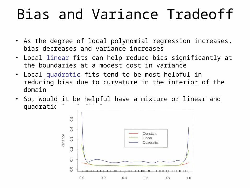
• As the degree of local polynomial regression increases, bias decreases and variance increases

• Local linear fits can help reduce bias significantly at the boundaries at a modest cost in variance

• Local quadratic fits tend to be most helpful in reducing bias due to curvature in the interior of the domain

• So, would it be helpful have a mixture or linear and quadratic local fits?

Local Regression in Higher Dimensions

• We can extend 1D local regression to higher dimensions

• Standardize each coordinates in the kernel, because Euclidean (square) norm is affected by scaling

ii

pp

Tdp

N

iii

TTTT

N

i

Tiii

xx

xxKithxWNN

xbithBHN

xbH

p

yxl

yxWBBxWBxbxxbxf

xxDxxK

xxbyxxK

,element diagonal with matrix diagonal

row with matrix regression

:function valued- vector 1

degree dwith dimension

ˆˆ

,

,min

00

T1

1

10

0

1

00000

00

2

100

, 00

Local Regression: Issues in Higher Dimensions

• The boundary poses even a greater problem in higher dimensions– Many training points are required to reduce the bias; Sample

size should increase exponentially in p to match the same performance.

• Local regression becomes less useful when dimensions go beyond 2 or 3

• It’s impossible to maintain localness (low bias) and sizeable samples (low variance) in the same time

Combating Dimensions: Structured Kernels

• In high dimensions, input variables (i.e., x variables) could be very much correlated. This correlation could be a key to reduce the dimensionality while performing kernel regression.

• Let A be a positive semidefinite matrix (what does that mean?). Let’s now consider a kernel that looks like:

• If A=-1, the inverse of the covariance matrix of the input variables, then the correlation structure is captured

• Further, one can take only a few principal components of A to reduce the dimensionality

00

0, ,xxAxx

DxxKT

A

Combating Dimensions: Low Order Additive Models

• ANOVA (analysis of variance) decomposition:

• One-dimensional local regression is all needed:

p

jjjp xgxxxf

121 ,,,

...,,,,1

21 lk

lkkl

p

jjjp xxgxgxxxf

Probability Density Function Estimation

• In many classification or regression problems we desperately want to estimate probability densities– recall the instances

• So can we not estimate a probability density, directly given some samples from it?

• Local methods of Density Estimation:

• This estimate is typically bumpy, non-smooth (why?)

ix

00

# ( )( ) ix Nbhood x

f xN

Smooth PDF Estimation using Kernels

• Parzen method:

• Gaussian kernel:

• In p-dimensions

N

iixxK

Nxf

100 ),(

1)(ˆ

20

1(|| ||/ )

20

12 2

1( )

(2 )

iN x x

X pi

f x e

N

)2

)(exp(

2

1),(

2

20

0 i

i

xxxxK

Kernel density estimation

Using Kernel Density Estimates in Classification

)|()( jGxpxf j

K

lll

jj

xf

xfxXjGP

10

00

)(ˆ

)(ˆ)|(

Posterior probability density:

In order to estimate this density, we can estimate the class conditional densitiesusing Parzen method

where is the jth class conditional density

Class conditional densities Ratio of posteriors )(ˆ)(ˆ

)|1(

)|1(

22

11

xf

xf

xXGP

xXGP

Naive Bayes Classifier

• In Bayesian Classification we need to estimate the class conditional densities:

• What if the input space x is multi-dimensional?

• If we apply kernel density estimates, we will run into the same problems that we faced in high dimensions

• To avoid these difficulties, assume that the class conditional density factorizes:

• In other words we are assuming here that the features are independent – Naïve Bayes model

• Advantages:– Each class density for each feature can

be estimated (low variance)– If some of the features are continuous,

some are discrete this method can seamlessly handle the situation

• Naïve Bayes classifier works surprisingly well for many problems (why?)

)|()( jGxpxf j

p

iipj jGxpxxf

11 )|(),,(

Discriminant function is now generalized linear additive

Key Points

• Local assumption• Usually Bandwidth () selection is more important than

kernel function selection• Low bias, low variance usually not guaranteed in high

dimensions• Little training and high online computational complexity

– Use sparingly: only when really required, like in the high-confusion zone

– Use when model may not be used again: No need for the training phase