Large Lump Detection by SVM Sharmin Nilufar Nilanjan Ray.
26
Large Lump Detection by SVM Sharmin Nilufar Nilanjan Ray
-
date post
21-Dec-2015 -
Category
Documents
-
view
226 -
download
0
Transcript of Large Lump Detection by SVM Sharmin Nilufar Nilanjan Ray.
Large Lump Detection by SVM
Sharmin Nilufar
Nilanjan Ray
Outline
• Introduction
• Proposed classification method– Scale space analysis of LLD images– Feature for classification
• Experiments and results
• Conclusion
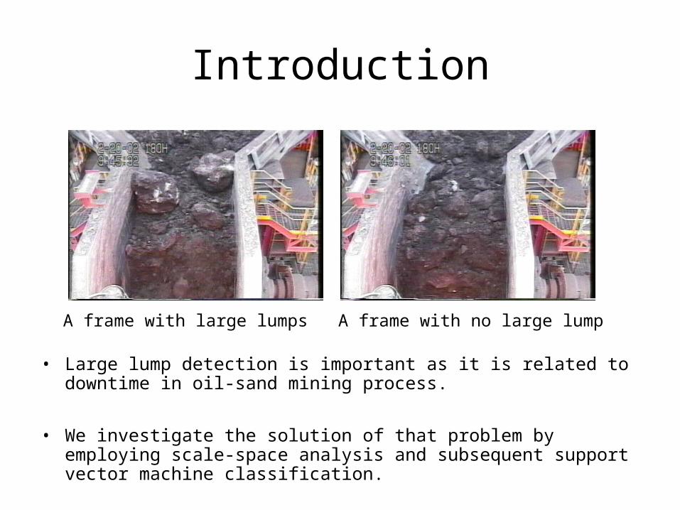
Introduction
• Large lump detection is important as it is related to downtime in oil-sand mining process.
• We investigate the solution of that problem by employing scale-space analysis and subsequent support vector machine classification.
A frame with large lumps A frame with no large lump
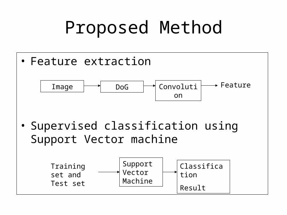
• Feature extraction
• Supervised classification using Support Vector machine
Proposed Method
Image DoG Convolution
Support Vector Machine
Classification
Result
Training set and Test set
Feature
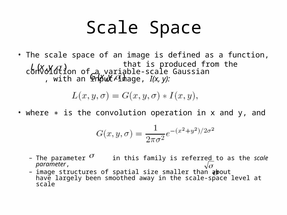
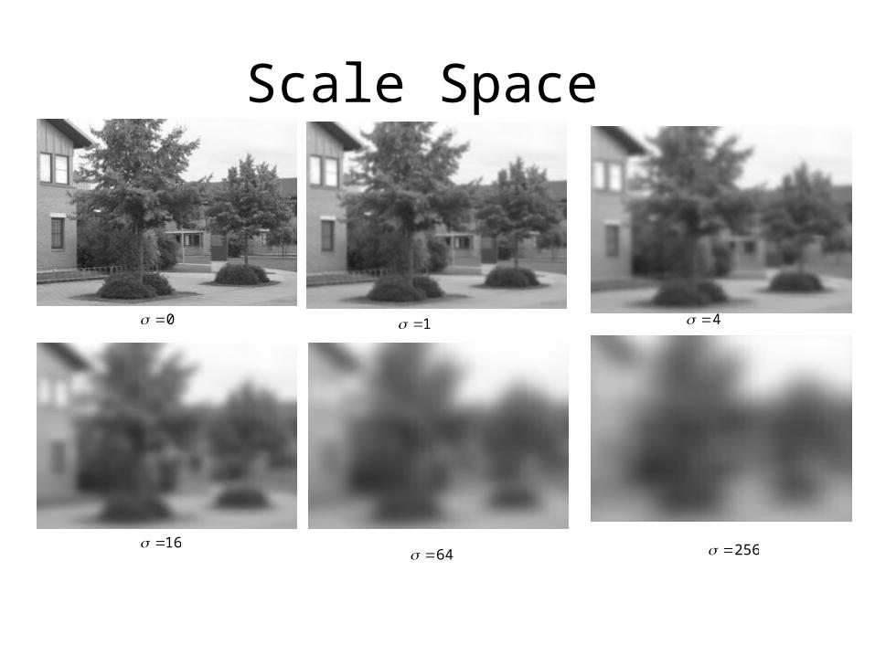
Scale Space
• The scale space of an image is defined as a function, that is produced from the convolution of a
variable-scale Gaussian , with an input image, I(x, y):
• where is the convolution operation in x and y, and∗
– The parameter in this family is referred to as the scale parameter, – image structures of spatial size smaller than about have largely
been smoothed away in the scale-space level at scale
),,( yxG),,( yxL
Scale Space
0
1
1 4
64 25616
Difference of Gaussian
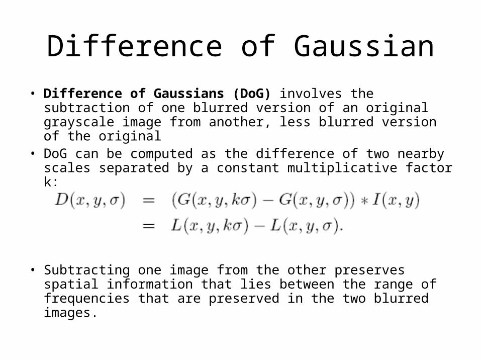
• Difference of Gaussians (DoG) involves the subtraction of one blurred version of an original grayscale image from another, less blurred version of the original
• DoG can be computed as the difference of two nearby scales separated by a constant multiplicative factor k:
• Subtracting one image from the other preserves spatial information that lies between the range of frequencies that are preserved in the two blurred images.
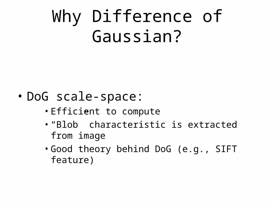
Why Difference of Gaussian?
• DoG scale-space:• Efficient to compute
• “Blob” characteristic is extracted from image
• Good theory behind DoG (e.g., SIFT feature)
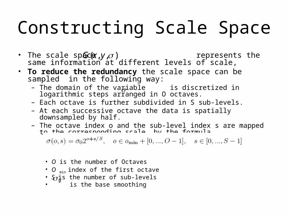
Constructing Scale Space• The scale space represents the same information at different
levels of scale,• To reduce the redundancy the scale space can be sampled in the
following way:– The domain of the variable is discretized in logarithmic steps arranged in O
octaves. – Each octave is further subdivided in S sub-levels.– At each successive octave the data is spatially downsampled by half. – The octave index o and the sub-level index s are mapped to the corresponding
scale by the formula
• O is the number of Octaves• O min index of the first octave • S is the number of sub-levels• is the base smoothing
),,( yxG
0
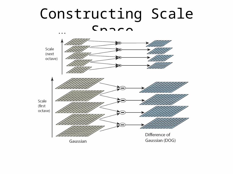
Constructing Scale Space…
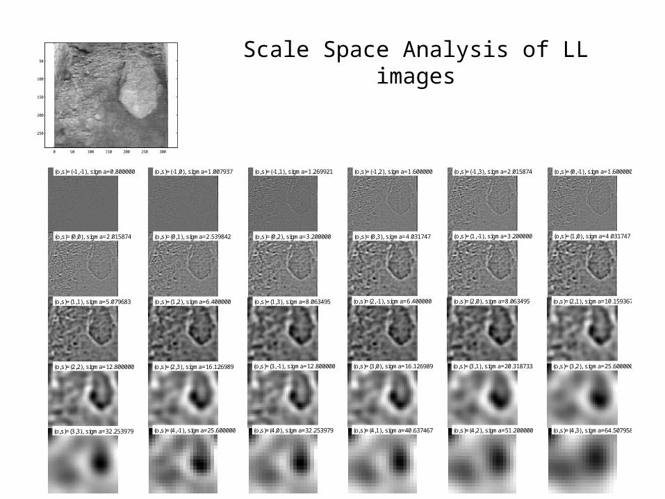
Scale Space Analysis of LL images
(o,s)=(-1,-1), sigma=0.800000 (o,s)=(-1,0), sigma=1.007937 (o,s)=(-1,1), sigma=1.269921 (o,s)=(-1,2), sigma=1.600000 (o,s)=(-1,3), sigma=2.015874 (o,s)=(0,-1), sigma=1.600000
(o,s)=(0,0), sigma=2.015874 (o,s)=(0,1), sigma=2.539842 (o,s)=(0,2), sigma=3.200000 (o,s)=(0,3), sigma=4.031747 (o,s)=(1,-1), sigma=3.200000 (o,s)=(1,0), sigma=4.031747
(o,s)=(1,1), sigma=5.079683 (o,s)=(1,2), sigma=6.400000 (o,s)=(1,3), sigma=8.063495 (o,s)=(2,-1), sigma=6.400000 (o,s)=(2,0), sigma=8.063495 (o,s)=(2,1), sigma=10.159367
(o,s)=(2,2), sigma=12.800000 (o,s)=(2,3), sigma=16.126989 (o,s)=(3,-1), sigma=12.800000 (o,s)=(3,0), sigma=16.126989 (o,s)=(3,1), sigma=20.318733 (o,s)=(3,2), sigma=25.600000
(o,s)=(3,3), sigma=32.253979 (o,s)=(4,-1), sigma=25.600000 (o,s)=(4,0), sigma=32.253979 (o,s)=(4,1), sigma=40.637467 (o,s)=(4,2), sigma=51.200000 (o,s)=(4,3), sigma=64.507958
0 50 100 150 200 250 300
50
100
150
200
250
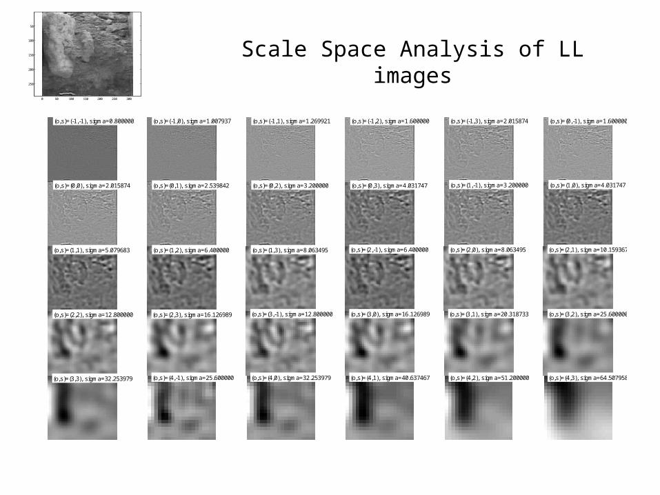
Scale Space Analysis of LL images
(o,s)=(-1,-1), sigma=0.800000 (o,s)=(-1,0), sigma=1.007937 (o,s)=(-1,1), sigma=1.269921 (o,s)=(-1,2), sigma=1.600000 (o,s)=(-1,3), sigma=2.015874 (o,s)=(0,-1), sigma=1.600000
(o,s)=(0,0), sigma=2.015874 (o,s)=(0,1), sigma=2.539842 (o,s)=(0,2), sigma=3.200000 (o,s)=(0,3), sigma=4.031747 (o,s)=(1,-1), sigma=3.200000 (o,s)=(1,0), sigma=4.031747
(o,s)=(1,1), sigma=5.079683 (o,s)=(1,2), sigma=6.400000 (o,s)=(1,3), sigma=8.063495 (o,s)=(2,-1), sigma=6.400000 (o,s)=(2,0), sigma=8.063495 (o,s)=(2,1), sigma=10.159367
(o,s)=(2,2), sigma=12.800000 (o,s)=(2,3), sigma=16.126989 (o,s)=(3,-1), sigma=12.800000 (o,s)=(3,0), sigma=16.126989 (o,s)=(3,1), sigma=20.318733 (o,s)=(3,2), sigma=25.600000
(o,s)=(3,3), sigma=32.253979 (o,s)=(4,-1), sigma=25.600000 (o,s)=(4,0), sigma=32.253979 (o,s)=(4,1), sigma=40.637467 (o,s)=(4,2), sigma=51.200000 (o,s)=(4,3), sigma=64.507958
0 50 100 150 200 250 300
50
100
150
200
250
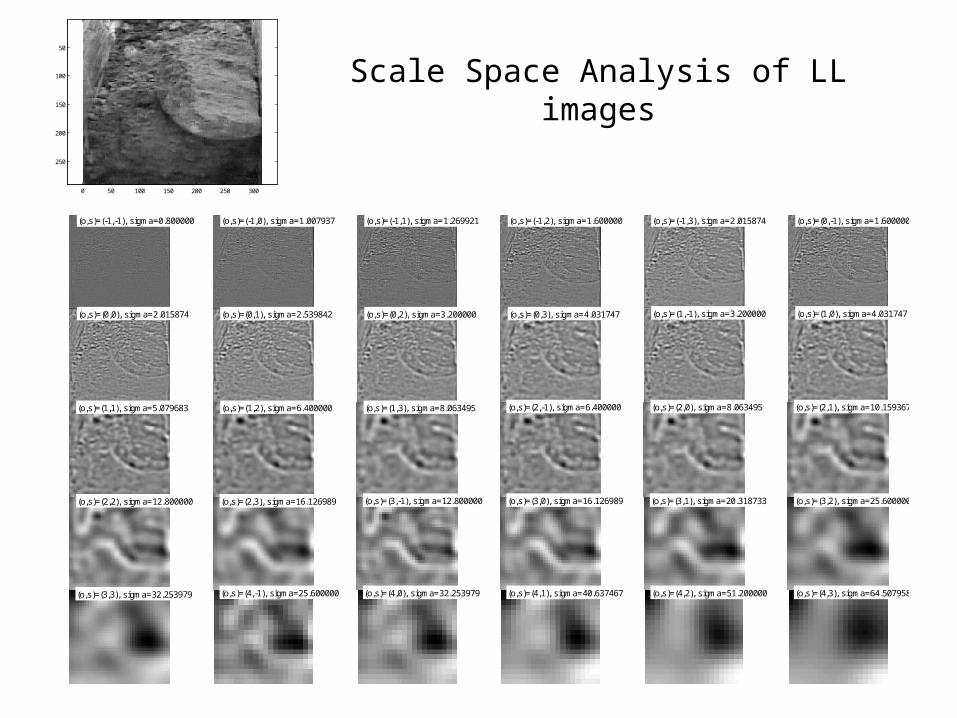
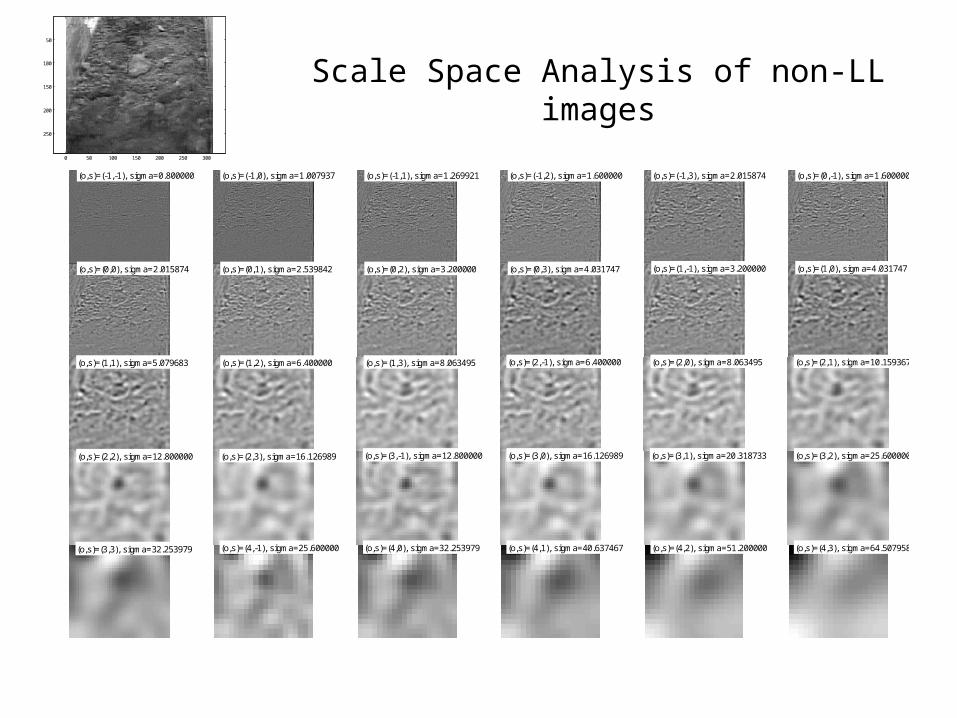
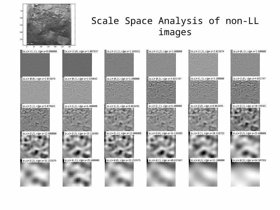
Scale Space Analysis of non-LL images
(o,s)=(-1,-1), sigma=0.800000 (o,s)=(-1,0), sigma=1.007937 (o,s)=(-1,1), sigma=1.269921 (o,s)=(-1,2), sigma=1.600000 (o,s)=(-1,3), sigma=2.015874 (o,s)=(0,-1), sigma=1.600000
(o,s)=(0,0), sigma=2.015874 (o,s)=(0,1), sigma=2.539842 (o,s)=(0,2), sigma=3.200000 (o,s)=(0,3), sigma=4.031747 (o,s)=(1,-1), sigma=3.200000 (o,s)=(1,0), sigma=4.031747
(o,s)=(1,1), sigma=5.079683 (o,s)=(1,2), sigma=6.400000 (o,s)=(1,3), sigma=8.063495 (o,s)=(2,-1), sigma=6.400000 (o,s)=(2,0), sigma=8.063495 (o,s)=(2,1), sigma=10.159367
(o,s)=(2,2), sigma=12.800000 (o,s)=(2,3), sigma=16.126989 (o,s)=(3,-1), sigma=12.800000 (o,s)=(3,0), sigma=16.126989 (o,s)=(3,1), sigma=20.318733 (o,s)=(3,2), sigma=25.600000
(o,s)=(3,3), sigma=32.253979 (o,s)=(4,-1), sigma=25.600000 (o,s)=(4,0), sigma=32.253979 (o,s)=(4,1), sigma=40.637467 (o,s)=(4,2), sigma=51.200000 (o,s)=(4,3), sigma=64.507958
0 50 100 150 200 250 300
50
100
150
200
250
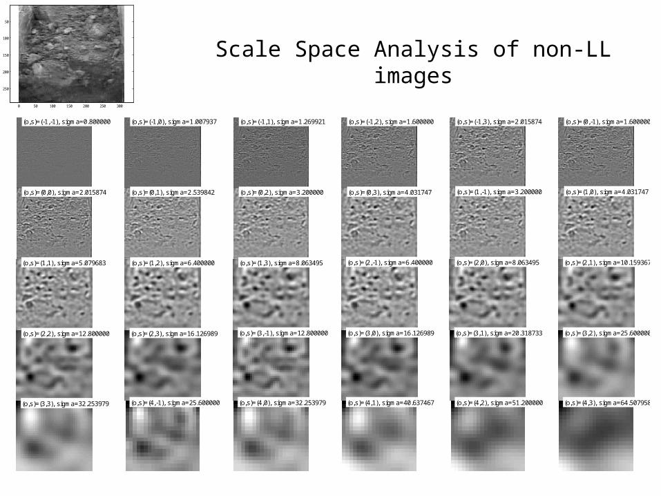
Scale Space Analysis of non-LL images
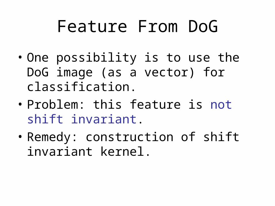
Feature From DoG
• One possibility is to use the DoG image (as a vector) for classification.
• Problem: this feature is not shift invariant.
• Remedy: construction of shift invariant kernel.
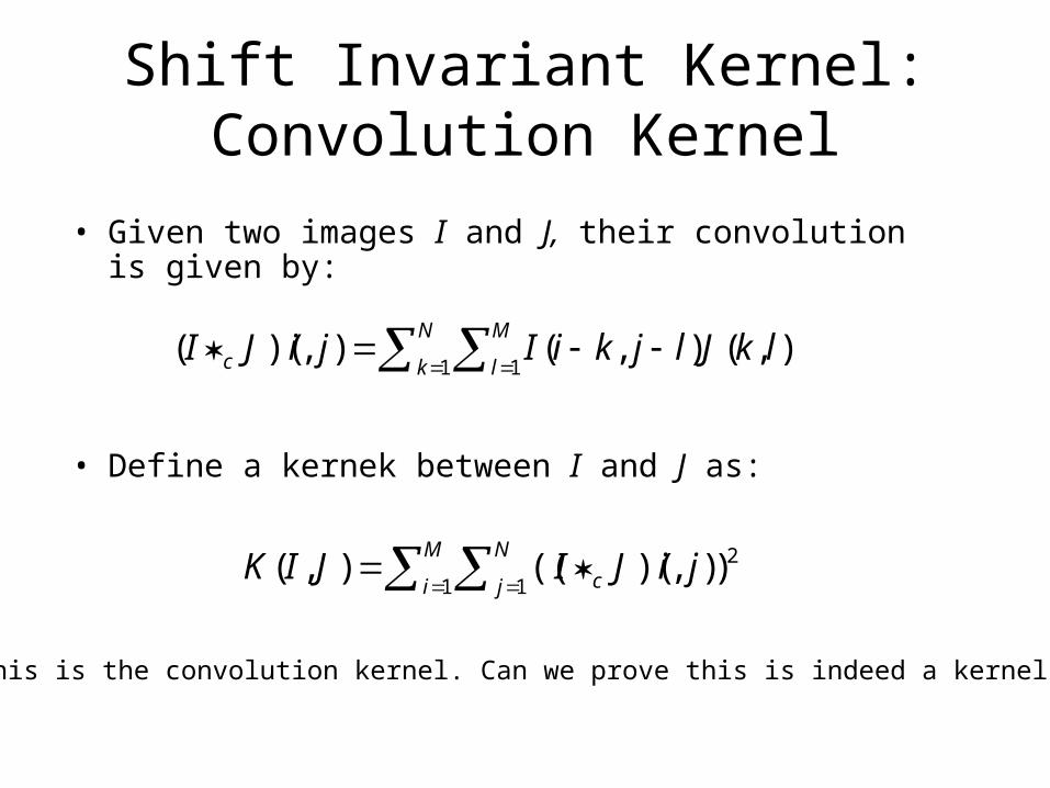
Shift Invariant Kernel: Convolution Kernel
• Given two images I and J, their convolution is given by:
• Define a kernek between I and J as:
N
k
M
lc lkJljkiIjiJI1 1
),(),(),)((
2
1 1)),)(((),(
M
i
N
j c jiJIJIK
This is the convolution kernel. Can we prove this is indeed a kernel?
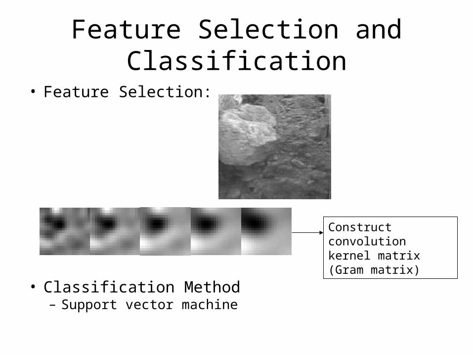
Feature Selection and Classification
• Feature Selection:
• Classification Method – Support vector machine
Construct convolution kernel matrix (Gram matrix)
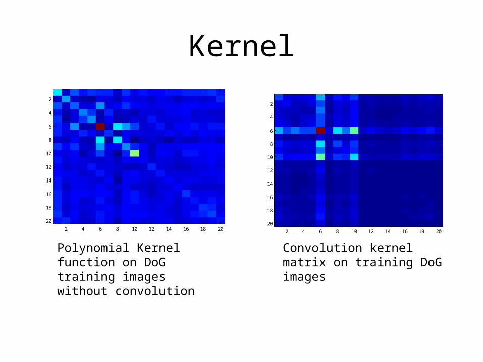
Kernel
2 4 6 8 10 12 14 16 18 20
2
4
6
8
10
12
14
16
18
20
2 4 6 8 10 12 14 16 18 20
2
4
6
8
10
12
14
16
18
20
Polynomial Kernel function on DoG training images without convolution
Convolution kernel matrix on training DoG images

Supervised Classification
• Classification Method- Support Vector Machine (SVM) with polynomial kernel– Using cross validation we got polynomial kernel of
degree 2 gives best results.
• Training set -20 image– 10 large lump images– 10 non large lump images
• Test Set -2446 images (training set including)– 45 large lumps
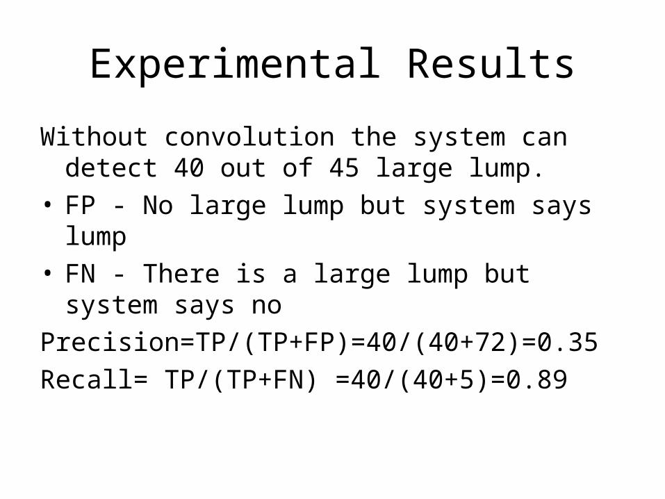
Experimental Results
Without convolution the system can detect 40 out of 45 large lump.
• FP - No large lump but system says lump• FN - There is a large lump but system says no
Precision=TP/(TP+FP)=40/(40+72)=0.35
Recall= TP/(TP+FN) =40/(40+5)=0.89
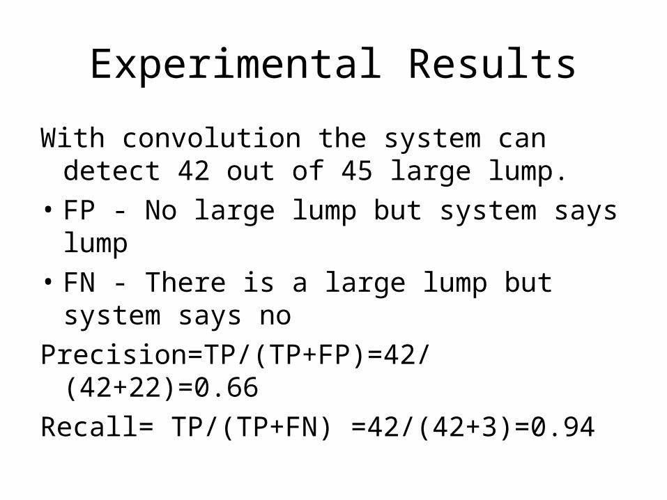
Experimental Results
With convolution the system can detect 42 out of 45 large lump.
• FP - No large lump but system says lump
• FN - There is a large lump but system says no
Precision=TP/(TP+FP)=42/(42+22)=0.66
Recall= TP/(TP+FN) =42/(42+3)=0.94
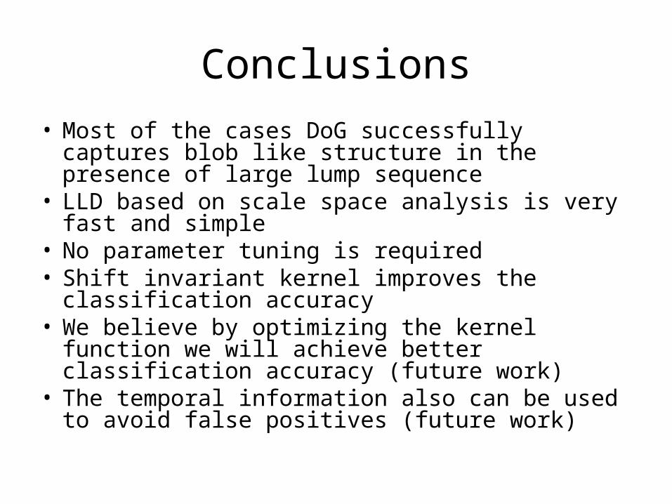
Conclusions
• Most of the cases DoG successfully captures blob like structure in the presence of large lump sequence
• LLD based on scale space analysis is very fast and simple
• No parameter tuning is required• Shift invariant kernel improves the classification
accuracy• We believe by optimizing the kernel function we will
achieve better classification accuracy (future work)• The temporal information also can be used to avoid
false positives (future work)
References
[1] Huilin Xiong Swamy M.N.S. Ahmad, M.O., “Optimizing the kernel in the empirical feature space”, IEEE Transactions on Neural Networks, 16(2), pp. 460-474, 2005.
[2] G. Lanckriet, N. Cristianini, P. Bartlett, L. E. Ghaoui, and M. I. Jordan, “Learning the kernel matrix with semidefinte programming,” J. Machine Learning Res., vol. 5, 2004.
[3] N. Cristianini, J. Kandola, A. Elisseeff, and J. Shawe-Taylor, “On kernel target alignment,” in Proc. Neural Information Processing Systems (NIPS’01), pp. 367–373.
[4] D. Lowe, "Object recognition from local scale-invariant features". Proceedings of the International Conference on Computer Vision pp. 1150–1157.,1999
Thanks