HAL Id: hal-01004965https://hal.archives-ouvertes.fr/hal-01004965

Submitted on 24 Jun 2019

HAL is a multi-disciplinary open accessarchive for the deposit and dissemination of sci-entific research documents, whether they are pub-lished or not. The documents may come fromteaching and research institutions in France orabroad, or from public or private research centers.

L’archive ouverte pluridisciplinaire HAL, estdestinée au dépôt et à la diffusion de documentsscientifiques de niveau recherche, publiés ou non,émanant des établissements d’enseignement et derecherche français ou étrangers, des laboratoirespublics ou privés.

A variational formulation for the incrementalhomogenization of elasto-plastic composites

L. Brassart, Laurent Stainier, I. Doghri, L. Delannay

To cite this version:L. Brassart, Laurent Stainier, I. Doghri, L. Delannay. A variational formulation for the incrementalhomogenization of elasto-plastic composites. Journal of the Mechanics and Physics of Solids, Elsevier,2011, 59 (12), pp.2455-2475. �10.1016/j.jmps.2011.09.004�. �hal-01004965�

A variational formulation for the incremental homogenization ofelasto-plastic composites

L. Brassart a, L. Stainier b, I. Doghri a, L. Delannay aa Universite catholique de Louvain, iMMC, 4 Av. Georges Lemaıtre, B-1348 Louvain-la-Neuve, Belgium b Ecole Centrale de Nantes, GeM (UMR 6183 CNRS), 1 Rue de la Noe, BP 92101, F-44321 Nantes, France

Keywords:MicromechanicsPlasticityHeterogeneous mediaParticle-reinforced composites

This work addresses the micro–macro modeling of composites having elasto-plasticconstituents. A new model is proposed to compute the effective stress–strain relationalong arbitrary loading paths. The proposed model is based on an incrementalvariational principle (Ortiz, M., Stainier, L., 1999. The variational formulation ofviscoplastic constitutive updates. Comput. Methods Appl. Mech. Eng. 171, 419–444)according to which the local stress–strain relation derives from a single incrementalpotential at each time step. The effective incremental potential of the composite is thenestimated based on a linear comparison composite (LCC) with an effective behaviorcomputed using available schemes in linear elasticity. Algorithmic elegance of the time-integration of J2 elasto-plasticity is exploited in order to define the LCC. In particular,the elastic predictor strain is used explicitly. The method yields a homogenized yieldcriterion and radial return equation for each phase, as well as a homogenized plasticflow rule. The predictive capabilities of the proposed method are assessed againstreference full-field finite element results for several particle-reinforced composites.

1. Introduction

The prediction of the effective behavior of composite materials with elasto-plastic components is efficiently addressedby micromechanical approaches. According to the latter, the macroscopic mechanical response is defined as the relationbetween volume averages of stress and strain fields at the lower scale. Such modeling explicitly accounts for internalstresses which in turn affect the overall (anisotropic) yield surface and hardening. This paper focuses on the developmentof a semi-analytical homogenization model suitable for large-scale simulations of composite parts and structures.

In the linear elastic regime, the effective stress–strain relation is fully characterized by the overall stiffness tensor, to becomputed once and for all from the elastic constants of the components given a statistical description of themicrostructure. The problem can be equivalently restated into that of determining per-phase averages of the stress(or equivalently strain) field. Among well-known schemes one may cite Hashin–Shtrikman bounds (Hashin and Shtrikman,1963; Willis, 1977), or the self-consistent (Kroner, 1958; Hill, 1965b) and Mori–Tanaka (Mori and Tanaka, 1973;Benveniste, 1987) approximations.

1

In contrast, when plastic deformation develops, mechanical properties do not remain homogeneous within phases, andthe local behavior becomes stress-dependent and history-dependent. Consequently, localization models valid in linearelasticity can no longer be applied. A workaround consists in considering a uniform plastic strain for each phase. Theproblem can then be handled within the framework of the transformation field analysis (TFA) (Dvorak and Benveniste,1992; Dvorak, 1992) and elastic localization rules are applicable, considering the plastic strain as a (given) eigenstrain.Updates of the plastic strain are computed at each time step from the constitutive equations of the phase using the firstmoment of the stress within the phase. However, the method yields too stiff predictions (Suquet, 1997; Chaboche et al.,2001, 2005) unless each plastic region is subdivided into sub-domains in order to capture plastic strain heterogeneities,which obviously increases the model complexity. Still treating the plastic strain as an eigenstrain, Buryachenko (1999)developed alternative elastic interaction laws based on a statistical approach, and used second moments of the stress toevaluate the yield condition in each phase.

An alternative strategy consists in linearizing the local stress–strain relation around some reference state (usuallychosen as the average deformation in the phase). This defines instantaneous, uniform properties for each phase. In theincremental method of Hill (1965a), tangent operators are used for the localization step in order to account for plasticaccommodation in the redistribution of the stress and strain (increments) among the phases (see also Hutchinson, 1970;Turner and Tome, 1994). Following Hill, other formulations based on linearized stress–strain relations were proposed, suchas secant methods (Berveiller and Zaoui, 1979; Tandon and Weng, 1988) and non-incremental tangent formulations forviscoplasticity (Hutchinson, 1976; Molinari et al., 1987; Lebensohn and Tome, 1993). An affine formulation for rate-independent elasto-plasticity was also proposed by Masson et al. (2000). Hill’s incremental formulation is particularly wellsuited for elasto-plasticity, as it preserves the incremental structure of the constitutive equations at both phase andmacroscopic levels. On the contrary, secant methods apply to plastic behavior only within a total deformation formalism.

It is well-recognized that both classical tangent and secant formulations yield too stiff responses (Gilormini, 1995;Suquet, 1996, 1997), and may even violate rigorous bounds obtained in the context of nonlinear elasticity by variationalapproaches, like those of Ponte Castaneda (1991). The reason for the overestimation might be attributed to the use ofuniform linearized properties for each plastic phase. This observation motivated the development of methods which usesecond moments of the stress (or strain) to account for field fluctuations within the phases. A modified secant theory wasproposed by Suquet (1995), which actually coincides with the variational procedure of Ponte Castaneda (1991) (Suquet,1995; Ponte Castaneda and Suquet, 1998). In the context of incremental tangent methods, overly stiff predictions may beavoided by defining the linearized properties using isotropic tangent moduli, instead of anisotropic ones (Gonzalez andLLorca, 2000; Doghri and Ouaar, 2003). This heuristic approach provides accurate predictions in many cases (Doghri andFriebel, 2005; Chaboche et al., 2005; Pierard et al., 2007). Some theoretical justifications for the use of isotropized tangentoperators are found in Chaboche and Kanoute (2003), Chaboche et al. (2005), and Pierard and Doghri (2006).

Recently, Lahellec and Suquet (2007a,b) proposed an incremental variational formulation for materials with a hereditarybehavior described by two potentials: a free energy and a dissipation function. It exploits an incremental variationalformulation for the local behavior (Ortiz and Stainier, 1999) according to which the stress can be derived from a singleincremental pseudo-potential. The effective behavior of the heterogeneous medium is then estimated following avariational formulation of the homogenization problem at each time step. A linear comparison composite (LCC) is definedbased on a linearization of the dissipation potential and the introduction of piecewise uniform, reference internal variables.The proposed linearizations inspire respectively from the variational procedure of Ponte Castaneda (1991) (Lahellec andSuquet, 2007a) and the second-order method of Ponte Castaneda (1996) (Lahellec and Suquet, 2007b). The approach seemsvery promising, although estimates were so far presented within the context of nonlinear viscoelasticity only.

The present work is also based on the incremental variational principle of Ortiz and Stainier (1999), but the adoptedstrategy to introduce the LCC is different from Lahellec and Suquet. The new procedure exploits the concept of trial straininvolved in the return mapping algorithm of J2 elasto-plasticity. The paper is organized as follows. Section 2 is a short,original presentation of the incremental variational principle of Ortiz and Stainier (1999) applied to small strain elasto-plasticity. In Section 3, the homogenization problem is formulated by adopting a variational formalism in a time-discretized setting. Section 4 proposes an alternative and yet equivalent formulation of the problem based on a LCC. Theformulation suggests an original localization rule based on the trial state. Based on this representation, a simple estimate isproposed in Section 5. Applications to two-phase particulate composites with highly contrasted phase properties arepresented in Section 6. The model provides satisfying predictions of the effective response in most cases, and is able tosustain cyclic loads.

Throughout the paper, Einstein’s convention is used, with indices ranging from 1 to 3, unless otherwise indicated. Theproducts of tensors are expressed as ðA : rÞij ¼ Aijklslk, ðr : rÞ ¼ sijsji, and ðr% rÞijkl ¼ sijskl. The symbols 1 and I stand forthe second and symmetric fourth order identity tensors, respectively. The spherical and deviatoric operators Ivol and Idev

are given by

Ivol & 131% 1, Idev & I'Ivol: ð1Þ

The von Mises measures of stress and strain are respectively given by

seq ¼ ð32 s : sÞ1=2 and eeq ¼ ð23e : eÞ1=2, ð2Þ

2

where s and e denote the deviatoric parts of r and e:

s¼ Idev : r, e¼ Idev : e: ð3Þ

2. Local constitutive equations

We focus on materials whose local response can be described by classical J2 elasto-plastic theory with isotropichardening. The behavior is assumed to be rate-independent and thermal effects are not considered. The constitutiveequations are written within the framework of Generalized Standard Media (Halphen and Nguyen, 1975; Germain et al.,1983), according to which state laws and complementary laws for the evolution of the internal variables respectivelyderive from a free energy and a dissipation function.

Time integration of the constitutive equations along a given path of applied deformation is performed according to anincremental variational principle. Numerous authors contributed to the development of variational principles equivalentto the incremental formulation of elasto-plasticity (e.g. Mialon, 1986; Comi et al., 1991; Martin et al., 1996; Carini, 1996;Ortiz and Stainier, 1999; Miehe, 2002). In particular, Ortiz and Stainier (1999) proposed a unified formulation providingupdates for the internal variables in the general context of elasto-(visco)plasticity at finite strains. On a time interval,updates of internal variables are obtained from the minimization of a suitably chosen functional, involving the free energyand the dissipation function. A remarkable advantage of the formulation is that the minimized functional constitutes aunique potential for the stress. This feature is the cornerstone of the homogenization procedure proposed in the sequel.

This section gives an extensive description of the incremental variational principle of Ortiz and Stainier (1999) in thecase of small strain elasto-plasticity. In particular, the classical radial return scheme is shown to derive from this principle.

2.1. Thermodynamic framework

Under the small displacement hypothesis, the (symmetric) total strain tensor e is classically decomposed into an elasticand a plastic part:

e¼ eeþep: ð4Þ

The chosen set of state variables comprises the total strain e, the plastic strain ep and an additional scalar variable pdescribing isotropic hardening and related to the accumulation of plastic deformation.

Contrarily to classical formulations (as described for instance in Lemaıtre and Chaboche, 1990; Maugin, 1992), no yieldfunction is explicitly introduced. Instead, kinematic restrictions related to the plastic flow are postulated a priori. Based onthe expected plastic flow kinematics in von Mises plasticity, the rate of plastic strain is split into a direction N andamplitude _p:

_ep ¼ _pN, ð5Þ

where N is a kinematic variable1 satisfying the following constraints:

trðNÞ ¼ 0 and N : N ¼ 32: ð6Þ

The constraints on N ensure incompressibility of the plastic flow and uniqueness of decomposition (5). With such norm ofN, it is easy to check that: _p ¼ ðð2=3Þ_ep : _epÞ1=2, so that the scalar variable p is the classical accumulated plastic strain. Thekinematic variable N will be specified later.

Supposing that the elastic response is independent of irreversible processes, the Helmholtz free energy (per unitvolume) admits the following additive decomposition:

cðe,ep,pÞ ¼ceðe'epÞþcpðpÞ: ð7Þ

The elastic part ce represents the energy stored within the material and recoverable through elastic relaxation. A linearresponse in the elastic regime is obtained by taking ce quadratic in the elastic strain:

ceðe'epÞ ¼ 12ðe'e

pÞ : Ce : ðe'epÞ, ð8Þ

where Ce is the elastic stiffness operator. The plastic part cp describing (isotropic) hardening is written as

cpðpÞ ¼Z p

0RðqÞ dq, ð9Þ

where R(q) represents the hardening stress (the function R is supposed to be given). Kinematic hardening can be modeledby including a dependence of the plastic potential on the plastic strain ep. However, kinematic hardening is not consideredin the homogenization model proposed here.

1 The kinematic variable N represents the direction of plastic flow. It should not be confused with some kinematic variable for the description ofkinematic hardening. The latter is not considered in the present work.

3

The state law for the stress is obtained from the free energy as

r¼@c@e

ðe,ep,pÞ ¼ '@c@ep

ðe,ep,pÞ ¼@ce

@eeðe'epÞ: ð10Þ

Hence, the stress is the force associated with both the total strain and the plastic strain. Similarly, the so-called hardeningstress is the thermodynamic force associated with the internal variable p:

R¼@c@p

ðe,ep,pÞ ¼@cp

@pðpÞ: ð11Þ

State laws (10) and (11) must be supplemented by a kinetic relation prescribing the evolution of the internal variable p(the evolution of ep being given by the flow rule (5)). The complementary law must ensure that the mechanical dissipationD is non-negative. Here, the dissipation expresses as (e.g. Lemaıtre and Chaboche, 1990):

D¼ r : _ep'R _pZ0: ð12Þ

The dissipation may conveniently be rewritten in a condensed form that accounts for the flow rule (5):

D¼ YðNÞ _p, ð13Þ

where the function Y is defined, for a given state fe,ep,pg, asYðNÞ ¼ r : N'R: ð14Þ

Expression (13) of the dissipation indicates that the new scalar quantity Y is the force conjugated to p, when it is computedfor the actual flow direction N. Then, the evolution law for p can be expressed as a kinetic relation between Y and _p. Basedon the theory of Generalized Standard Media, it is supposed to derive from a dissipation function fð _pÞ:

Y ¼@f@ _p

ð _pÞ or, equivalently _p ¼@fn

@YðYÞ, ð15Þ

where fn is the convex dual of f by Legendre transform:

fnðYÞ ¼ sup_pf _pY'fð _pÞg: ð16Þ

By choosing fð _pÞ non-negative, convex and such that fð0Þ ¼ 0, the mechanical dissipation (13) is necessarily positive.

Remark 1. The comparison between Y and a thermodynamic force can be further justified on energy basis. Considervirtual (and independent) perturbations p-pþdp and ep-epþdep, with dep & ~Ndp, ~N being an arbitrary flow direction.The total deformation is kept constant. The corresponding variation of the free energy is then

dc¼@ce

@ee:@ee

@ep: depþ

@cp

@pdp

! "&'Yð ~N Þdp: ð17Þ

Thus, the quantity Yð ~N Þdp measures the variation of free energy at constant total deformation, for a given variation of pand an arbitrary direction of plastic flow ~N .

The classical equations of rate-independent elasto-plasticity are retrieved by taking the dissipation function homo-geneous of degree one with respect to (w.r.t.) _p:

fð _pÞ ¼sY _p, _pZ0,

þ1 otherwise:

(

ð18Þ

Since f is not differentiable at _p ¼ 0, the partial derivative in (15) must be understood in the sense of sub-differential(Rockafellar, 1970; Moreau, 1976). The kinetic relation (15) yields

YosY 3 _p ¼ 0,

Y ¼ sY 3 _pZ0: ð19Þ

In other words, deformations are purely elastic when the forces are inside an elasticity domain ½0,sY ½. Plastic flow occurswhen the force Y reaches the yield stress sY . In addition, Y cannot leave the yield surface when plastic deformation occurs( _p40). On the other hand, negative values of _p are prohibited, as they would imply infinite dissipation. The function fð _pÞdefines a convex set whose indicator function is precisely the dual fn of f (see e.g. Maugin, 1992), which is here given by

fnðYÞ ¼0, YrsY ,

þ1 otherwise:

(ð20Þ

This convex set precisely coincides with the elasticity domain just introduced. Thus, the existence of an elasticity domainfollows from the definition of the dissipation function.

The kinematic variable N was not specified up to now. Actually, it can be shown that N is found by maximizing thedissipation at fixed p and _p. This follows from a continuous variational principle introduced by Ortiz and Stainier (1999),

4

which is not presented here for brevity. The kinematic variable will be specified within the discretized formulationpresenter hereafter.

2.2. Incremental variational principle

We now consider the problem of integrating the constitutive relations over a time increment ½tn,tnþ1). The state at tn issupposed to be given: fen,e

pn,png, so as the total deformation at tnþ1 : enþ1. We aim to compute the stress rnþ1, the plastic

strain epnþ1 and the accumulated plastic strain pnþ1 at tnþ1. We first assume that the rate of accumulated plastic strain _p isconstant over the time step and given by the ratio Dp=Dt, with Dð*Þ ¼ ð*Þnþ1'ð*Þn. Similarly, the plastic flow rule (5) isdiscretized as

Dep ¼DpN, ð21Þ

where N is an (a priori unknown) constant plastic flow direction for the time step. Ortiz and Stainier (1999) proposed thefollowing incremental variational principle:

WDðenþ1Þ ¼ infDp,N

JDðenþ1,Dp,NÞ, ð22Þ

where the minimization w.r.t. N is performed under constraints (6) and

JDðenþ1,Dp,NÞ ¼cðenþ1,epnþ1,pnþ1Þ'cnþDtf Dp

Dt

! ", ð23Þ

where epnþ1 is obtained from the discretized flow rule (21) and cn is the free energy computed for the (given) statevariables at tn. Then, considering the stationarity conditions w.r.t. Dp and N in (22), the stress tensor at tnþ1 is given by

rnþ1 ¼dWD

denþ1ðenþ1Þ ¼

@JD@enþ1

ðenþ1,Dp,NÞ, ð24Þ

where Dp and N are the solutions of the minimization problem (22). Thus, the functionWD plays the role of an incrementalpotential for the stress. In the following we show that the optimality conditions w.r.t. Dp and N yield the classicalincremental relations of J2 plasticity. In particular, the well-known radial return scheme with its predictor and correctorsteps (Wilkins, 1964, see also Simo and Hughes, 1998 or Doghri, 2000) is retrieved.

Taking into account the discretized flow rule (21), the stationarity condition of JD w.r.t. Dp gives the discretized kineticrelation (15):

Ynþ1ðN,pnþ1Þ ¼@f@ _p

DpDt

! ", ð25Þ

where the function Ynþ1 is defined similarly as in the continuous case (14):Ynþ1ðN,pnþ1Þ & rnþ1 : N'Rðpnþ1Þ: ð26Þ

Note that rnþ1 now depends on N, since:

rnþ1 ¼@ce

@eeðeenþ1Þ with eenþ1 ¼ enþ1'epn'DpN: ð27Þ

Therefore, it is conveniently rewritten as

rnþ1 ¼ Ce : ðetrnþ1'DpNÞ ¼ rtrnþ1'DpðC

e : NÞ, ð28Þ

introducing the trial (or predictor) elastic strain etrnþ1 and the corresponding trial stress:

etrnþ1 & enþ1'epn, ð29Þ

rtrnþ1 & Ce : etrnþ1: ð30Þ

The minimization of JD w.r.t. N under constraints (6) is performed using Lagrange multipliers and it yields (seeAppendix A)

N ¼32

strnþ1

streq,nþ1

¼etr

etreq: ð31Þ

Expression (31) of the kinematic variable is obtained assuming isotropic elasticity, in which case the elastic stiffness tensoradmits the following decomposition:

Ce ¼ 3kIvolþ2mIdev, ð32Þ

where k and m are the elastic bulk and shear moduli, respectively.Substituting (31) into (26), the stationarity condition (25) for Dp becomes

'3metreq,nþ1þ3mDpþRðpnþ1Þþ@f@ _p

DpDt

! "¼ 0: ð33Þ

5

The problem of the non-smoothness of the dissipation function for Dp¼ 0 can be circumvented by first evaluating theslope of the functional JD for Dp¼ 0þ . If it is negative, that is

'3metreq,nþ1þRðpnÞþsY o0, ð34Þ

then the optimal Dp is positive, and satisfies the following equation:

'3metreq,nþ1þ3mDpþRðpnþDpÞþsY ¼ 0: ð35Þ

Otherwise, the optimal Dp is zero, as negative values are prohibited (they would lead to infinite dissipation), and the incrementis elastic. Therefore, the minimization problem associated with the incremental variational principle involves the evaluation of ayield criterion in terms of an elastic predictor, and a plastic correction step, exactly like in the classical return mapping.

Remark 2. The incremental functionals WD and JD are related to a time increment and they depend on the past loadinghistory. Therefore, they are not state functions. For this reason, WD should preferably be referred to as a pseudo-potentialfor the stress.

3. Homogenization

3.1. Local potential

We consider a representative volume element (RVE) V of a composite with N elasto-plastic phases r¼1,y,N. Each phaseoccupies a domain Vr of the RVE with volume fraction cr ¼ Vr=V and characteristic function wðrÞ, with wðrÞðxÞ ¼ 1 if x is inphase r, and 0 elsewhere. The local constitutive behavior is characterized by a free energy and a dissipation function:

cðx,e,ep,pÞ ¼XN

r ¼ 1

wðrÞðxÞcðrÞðe,ep,pÞ, fðx, _pÞ ¼XN

r ¼ 1

wðrÞðxÞfðrÞð _pÞ, ð36Þ

where

cðrÞðe,ep,pÞ ¼ceðrÞðe'epÞþcpðrÞðpÞ, ð37Þ

ceðrÞðe'epÞ ¼ 12ðe'e

pÞ : CeðrÞ : ðe'epÞ, ð38Þ

CeðrÞ ¼ 3kðrÞIvolþ2mðrÞIdev, ð39Þ

cpðrÞðpÞ ¼Z p

0RðrÞðqÞ dq, ð40Þ

fðrÞð _pÞ ¼ _psðrÞY if _pZ0, þ1 otherwise: ð41Þ

Adopting the incremental setting of Section 2.2, and assuming the local state at tn to be given, the internal variables epnþ1and pnþ1, as well as the kinematic variable N are determined from the solution of the following local minimizationproblem at a given material point:

WDðx,enþ1Þ ¼ infDp,N

JDðx,enþ1,Dp,NÞ, ð42Þ

where the minimization w.r.t. N is performed under constraints (6). The functional JD is given by

JDðx,enþ1,Dp,NÞ ¼cðx,enþ1,epnþ1,pnþ1Þ'cnðxÞþDtf x,

DpDt

! ", ð43Þ

where epnþ1 depends on Dp and N through the incremental flow rule (21). Note that JD (and thus WD) depend on x not onlythrough the characteristic functions wðrÞ in (36), but also through the fields epnðxÞ and pnðxÞ. The function (42) acts as apotential for the stress:

rnþ1 ¼@WD

@enþ1ðenþ1Þ: ð44Þ

3.2. Effective behavior

Let / *S and / *Sr denote a volume average over the RVE and phase r, respectively, with / *S¼PN

r ¼ 1 cr/ *Sr . Weaim to compute the effective stress response of the composite rðtÞ &/rðtÞS for a given history of prescribed deformationeðtÞ &/eðtÞS. In the time-discretized setting, the effective behavior of the composite at time tnþ1 can be determined fromthe effective incremental energy function (Miehe, 2002; Lahellec and Suquet, 2007a):

WDðenþ1Þ & infenþ 12Kðenþ 1Þ

/WDðx,enþ1ÞS, ð45Þ

6

where the set Kðenþ1Þ of admissible strain fields is defined as

Kðenþ1Þ ¼ fenþ1 ¼ 12ðð=uÞnþ1þð=uÞTnþ1Þ,/enþ1S¼ enþ1g, ð46Þ

where u denotes the displacement field within the RVE. For definiteness of problem (45), boundary conditions satisfyingthe constraint on the average of the strain field in (46) must be imposed on the boundary of the RVE. Linear displacementboundary conditions such that unþ1 ¼ enþ1 * x on @V may be adopted. Periodic boundary conditions or surface tractionboundary conditions could alternatively be considered, see for instance Miehe (2002).

Eq. (45) defines an effective incremental potential for the composite WD from which the macroscopic stress is derived:

rnþ1 ¼/rnþ1S¼@WD

@enþ1ðenþ1Þ: ð47Þ

A proof of the latter equality is given by Lahellec and Suquet (2007a) and reads as follows. First, the derivative of WD w.r.t.enþ1 is computed:

@WD

@enþ1ðenþ1Þ ¼

@JD@enþ1

ðx,enþ1,anþ1Þ :@enþ1

@enþ1

# $þ

@JD@anþ1

ðx,enþ1,anþ1Þ :@anþ1

@enþ1

# $, ð48Þ

where anþ1 collectively denotes Dp and N, solutions of the minimization problem (42) at tnþ1. The second term on theright vanishes due to the stationarity of JD w.r.t. anþ1 (implicitly taking the kinematic constraints on N into account) andthe first one gives, thanks to Hill’s Lemma (Hill, 1967):

rnþ1 :@enþ1

@enþ1

# $¼/rnþ1S :

@enþ1

@enþ1

# $¼/rnþ1S¼ rnþ1: ð49Þ

Making use of expressions (36), (42) and (43), the effective incremental potential (45) is rewritten as

WDðenþ1Þ ¼ infenþ 12Kðenþ 1Þ

infDp,N

XN

r ¼ 1

wðrÞðxÞ cðrÞðenþ1,epnþ1,pnþ1Þ'cðrÞ

n ðxÞþDtfðrÞ DpDt

! "% &( )* +: ð50Þ

The solution fields Dp and N fluctuate within the composite, depending on the local strain enþ1 and state variables at tn, epn

and pn. Obviously, an exact semi-analytical solution for problem (50) is out of range and approximations are required.A straightforward simplification to problem (50) consists in considering piecewise uniform internal variables. As shown

in Appendix B, such simplification leads to the transformation field analysis (TFA): the strain field is computed on acomparison composite characterized by the elastic moduli, with the plastic strain acting as an eigenstrain. Updates of theinternal variables result from the incremental variational principle and obey a radial return scheme for each phase.However, it is well known that the predictions of the TFA are too stiff when it is applied to two-phase systems, because it isbased on purely elastic accommodation.

The homogenization model presented in the sequel is based on different linearized interaction relations. Inspiring fromthe variational technique of Ponte Castaneda (1991, 1992), an original linearization strategy is presented, according towhich the effective potential (50) is reexpressed in terms of the effective potential of a linear comparison composite (LCC)characterized by secant operators for the trial strain–stress relation. Based on this formulation, estimates of the effectivebehavior are proposed. In the remainder of the paper, all quantities are evaluated at tnþ1 (subscripts (nþ1) omitted forsimplicity), unless otherwise indicated.

4. Variational procedure: definition of a linear comparison composite

4.1. Phase potential

As a starting point, we consider that the infimum over the kinematic variable N in (50) is satisfied at each materialpoint in the composite, so that expression (31) may be used. Then, the elastic strain can be expressed as a function of thetrial strain and Dp as

ee ¼ etr'Dep ¼ etr'DpN with N ¼etr

etreq: ð51Þ

It follows that the hydrostatic and equivalent elastic strains can be rewritten as

eem ¼ etrm and eeeq ¼ 1'Dpetreq

!etreq, ð52Þ

where the hydrostatic strain is defined as: em & 13 trðeÞ. Now, consider the following expression for the elastic free energy (38):

ceðrÞðeeÞ ¼ 92 k

ðrÞðeemÞ2þ32m

ðrÞðeeeqÞ2: ð53Þ

7

Introducing relations (52) into the latter expression, the elastic free energy can be reexpressed in terms of the trial strain.It yields

ceðrÞðeeÞ &CeðrÞðetr ,DpÞ ¼ 92k

ðrÞðetrmÞ2þ f ðrÞððetreqÞ2,DpÞ, ð54Þ

where the function f(r) is given by

f ðrÞððetreqÞ2,DpÞ ¼32mðrÞ 1'

DpffiffiffiffiffiffiffiffiffiffiffiffiðetreqÞ2

q

0

B@

1

CA

2

ðetreqÞ2 ¼32mðrÞð

ffiffiffiffiffiffiffiffiffiffiffiffiðetreqÞ2

q'DpÞ2, ð55Þ

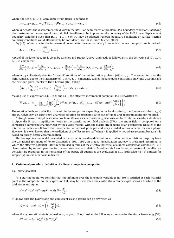
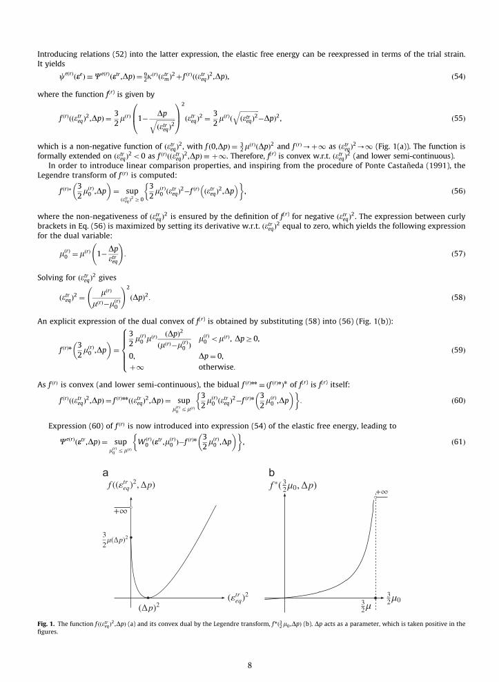
which is a non-negative function of ðetreqÞ2, with f ð0,DpÞ ¼ 32mðrÞðDpÞ2 and f ðrÞ-þ1 as ðetreqÞ2-1 (Fig. 1(a)). The function is

formally extended on ðetreqÞ2o0 as f ðrÞððetreqÞ2,DpÞ & þ1. Therefore, f(r) is convex w.r.t. ðetreqÞ2 (and lower semi-continuous).In order to introduce linear comparison properties, and inspiring from the procedure of Ponte Castaneda (1991), the

Legendre transform of f ðrÞ is computed:

f ðrÞ+32mðrÞ0 ,Dp

! "¼ sup

ðetreqÞ2 Z0

32mðrÞ0 ðetreqÞ2'f ðrÞ ðetreqÞ2,Dp

( )% &, ð56Þ

where the non-negativeness of ðetreqÞ2 is ensured by the definition of f(r) for negative ðetreqÞ2. The expression between curlybrackets in Eq. (56) is maximized by setting its derivative w.r.t. ðetreqÞ2 equal to zero, which yields the following expressionfor the dual variable:

mðrÞ0 ¼ mðrÞ 1'

Dpetreq

!: ð57Þ

Solving for ðetreqÞ2 gives

ðetreqÞ2 ¼mðrÞ

mðrÞ'mðrÞ0

!2

ðDpÞ2: ð58Þ

An explicit expression of the dual convex of f(r) is obtained by substituting (58) into (56) (Fig. 1(b)):

f ðrÞn32mðrÞ0 ,Dp

! "¼

32mðrÞ0 mðrÞ ðDpÞ2

ðmðrÞ'mðrÞ0 Þ

mðrÞ0 omðrÞ, DpZ0,

0, Dp¼ 0,

þ1 otherwise:

8>>>><

>>>>:

ð59Þ

As f ðrÞ is convex (and lower semi-continuous), the bidual f ðrÞnn & ðf ðrÞnÞn of f(r) is f(r) itself:

f ðrÞððetreqÞ2,DpÞ ¼ f ðrÞnnððetreqÞ2,DpÞ ¼ supmðrÞ0

rmðrÞ

32mðrÞ0 ðetreqÞ2'f ðrÞn

32mðrÞ0 ,Dp

! "% &: ð60Þ

Expression (60) of f ðrÞ is now introduced into expression (54) of the elastic free energy, leading to

CeðrÞðetr ,DpÞ ¼ supmðrÞ0

rmðrÞ

W ðrÞ0 ðetr ,mðrÞ

0 Þ'f ðrÞn32mðrÞ0 ,Dp

! "% &, ð61Þ

Fig. 1. The function f ððetreqÞ2 ,DpÞ (a) and its convex dual by the Legendre transform, f nð32m0 ,DpÞ (b). Dp acts as a parameter, which is taken positive in thefigures.

8

where W ðrÞ0 is similar in form to the elastic energy of a linear, isotropic material:

W ðrÞ0 ðetr ,mðrÞ

0 Þ ¼ 92 k

ðrÞðetrmÞ2þ32 m

ðrÞ0 ðetreqÞ2 ¼ 1

2 etr : CðrÞ

0 : etr ¼ 12ðe'e

pnÞ : C

ðrÞ0 : ðe'epnÞ, ð62Þ

with CðrÞ0 given by

CðrÞ0 ¼ 3kðrÞIvolþ2mðrÞ

0 Idev: ð63Þ

Therefore, the dual variable mðrÞ0 introduced by the Legendre transform plays the role of a shear modulus in a fictitious

linear elastic material with potential (62). Accordingly, it should be positive everywhere. It will be shown that it is indeedthe case according to the model proposed in the next section. Note that mðrÞ

0 fluctuates within phase r, according to itsexpression (57). On the other hand, the plastic strain epn plays the role of an eigenstrain field applied to the linearcomparison material.

The linearization suggested by the variational procedure can be interpreted as follows. Using expression (61) for theelastic part of the free energy, the local stress in the composite is given by

r¼@CeðrÞ

@etr:@etr

@ee¼ CðrÞ

0 : etr : ð64Þ

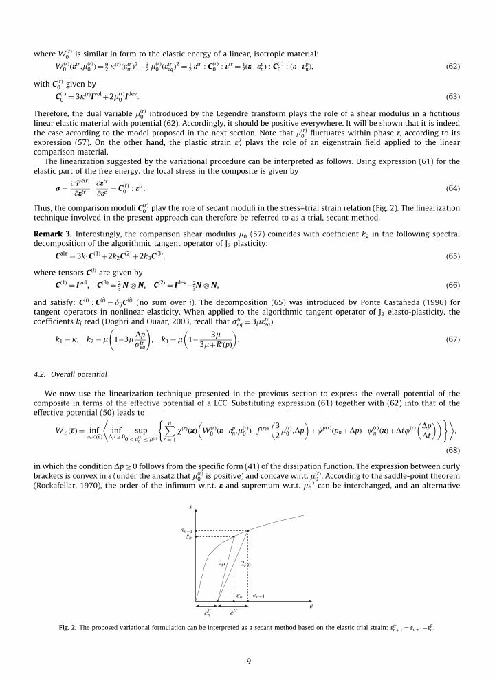
Thus, the comparison moduli CðrÞ0 play the role of secant moduli in the stress–trial strain relation (Fig. 2). The linearization

technique involved in the present approach can therefore be referred to as a trial, secant method.

Remark 3. Interestingly, the comparison shear modulus m0 (57) coincides with coefficient k2 in the following spectraldecomposition of the algorithmic tangent operator of J2 plasticity:

Calg ¼ 3k1Cð1Þ þ2k2C

ð2Þ þ2k3Cð3Þ, ð65Þ

where tensors CðiÞ are given by

Cð1Þ ¼ Ivol, Cð3Þ ¼ 23 N % N, Cð2Þ ¼ Idev'2

3N % N, ð66Þ

and satisfy: CðiÞ : CðjÞ ¼ dijCðiÞ (no sum over i). The decomposition (65) was introduced by Ponte Castaneda (1996) fortangent operators in nonlinear elasticity. When applied to the algorithmic tangent operator of J2 elasto-plasticity, thecoefficients ki read (Doghri and Ouaar, 2003, recall that str

eq ¼ 3metreqÞ

k1 ¼ k, k2 ¼ m 1'3m Dpstreq

!, k3 ¼ m 1'

3m3mþR0ðpÞ

! ": ð67Þ

4.2. Overall potential

We now use the linearization technique presented in the previous section to express the overall potential of thecomposite in terms of the effective potential of a LCC. Substituting expression (61) together with (62) into that of theeffective potential (50) leads to

WDðeÞ ¼ infe2KðeÞ

infDpZ0

sup0omðsÞ

0rmðsÞ

Xn

r ¼ 1

wðrÞðxÞ W ðrÞ0 ðe'epn,m

ðrÞ0 Þ'f ðrÞn

32mðrÞ0 ,Dp

! "þcpðrÞðpnþDpÞ'cðrÞ

n ðxÞþDtfðrÞ DpDt

! "! "( )* +

,

ð68Þ

in which the condition DpZ0 follows from the specific form (41) of the dissipation function. The expression between curlybrackets is convex in e (under the ansatz that mðrÞ

0 is positive) and concave w.r.t. mðrÞ0 . According to the saddle-point theorem

(Rockafellar, 1970), the order of the infimum w.r.t. e and supremum w.r.t. mðrÞ0 can be interchanged, and an alternative

Fig. 2. The proposed variational formulation can be interpreted as a secant method based on the elastic trial strain: etrnþ1 ¼ enþ1'epn .

9

representation is obtained:

WDðeÞ ¼ infDpZ0

sup0omðsÞ

0rmðsÞ

W 0ðe,mðsÞ0 Þþ

Xn

r ¼ 1

wðrÞðxÞ 'f ðrÞn32mðrÞ0 ,Dp

! "þcpðrÞðpnþDpÞ'cðrÞ

n ðxÞþDtfðrÞ DpDt

! "! "* +( )

, ð69Þ

where W 0 is the effective potential of a LCC characterized by phase potentials W ðrÞ0 :

W 0ðe,mðsÞ0 Þ ¼ inf

e2KðeÞ

Xn

r ¼ 1

wðrÞðxÞW ðrÞ0 ðe'epn,m

ðrÞ0 Þ

* +

: ð70Þ

The expression between curly brackets in (69) is not convex w.r.t. Dp, so that the order of the infimum and supremumoperations may not be inverted. Accounting for the stationarity w.r.t. the fields mðrÞ

0 and Dp, the overall stress of thecomposite is given by

r ¼@WD

@eðeÞ ¼

@W 0

@eðe,mðsÞ

0 Þ: ð71Þ

The formulation (69) of the homogenization problem, supplemented by the local flow rule (21), is completely equivalent tothe original one (50), and is therefore as complicated to solve. However, it involves the effective energy of a LCC, whichconstitutes the first step towards the derivation of estimates.

4.3. Approximation by piecewise uniform shear moduli

A straightforward (and probably unavoidable) approximation to formulation (69) consists in considering piecewiseuniform shear moduli within the LCC:

m0ðxÞ ¼XN

r ¼ 1

wðrÞðxÞmðrÞ0 , ð72Þ

where mðrÞ0 is now uniform in phase r. This corresponds to a restriction of the solutions space in the variational problem

(69). In (72), it is assumed that the spatial distribution of the phases in the LCC coincides with the one in the actualcomposite.2

Approximation (72) also implies piecewise uniformity of the optimal field DpðxÞ, solution of the variational problem(69). Indeed, consider the composite in a strain- and stress-free configuration at t¼t0, so that pn is initially piecewiseuniform (and zero). As all terms involving p and/or Dp in the functional between curly brackets in Eq. (69) are piecewiseuniform, it follows that DpðxÞ solution of the infimum problem at t1 is also piecewise uniform. Applying the samereasoning at each subsequent time step, the fields DpðxÞ, as well as pðxÞ at any time tnþ1 are necessarily piecewise uniform.

5. An estimate based on uniform eigenstrain

The piecewise uniformity of the shear moduli and the internal variable p (as a consequence) dramatically reduces thedifficulty of problem (69). However, the eigenstrain field epn in (70) fluctuates within each plastic phase, preventing a directapplication of linear estimates for thermoelastic composites. Therefore, an additional approximation is required, whichmight consist in considering a uniform, reference plastic strain at tn for each phase in expression (70). A rather intuitivechoice is to set the reference plastic strain equal to the average of the plastic strain in the phase. Unfortunately, resultsobtained so far under this assumption turned out to be inconsistent in most examples of particulate composites reinforcedby elastic inclusions (Brassart, 2011).

The estimate proposed and validated in the sequel is based on a different, and yet simpler modeling assumption of auniform reference plastic strain for the whole composite. The effective potential (70) of the LCC is then approximated as

W 0ðe,mðsÞ0 Þ , ~W 0ðe,mðsÞ

0 Þ ¼ infe2KðeÞ

Xn

r ¼ 1

wðrÞðxÞW ðrÞ0 ðe'epn,m

ðrÞ0 Þ

* +, ð73Þ

where epn is the reference plastic strain, given by

epn &/epnS: ð74Þ

Then, the effective potential of the LCC is simply given by~W 0ðe,mðsÞ

0 Þ ¼ 12ðe'/epnSÞ : C0 : ðe'/epnSÞ, ð75Þ

where C0 is the overall elastic stiffness of the LCC, to be computed from any linear scheme suited for the microstructureunder consideration.

2 This prescription is not absolutely necessary, nor necessarily optimal, as noted by Suquet (1993). However, the question of considering a LCC with amicrostructure different from the actual one is not investigated in the present work.

10

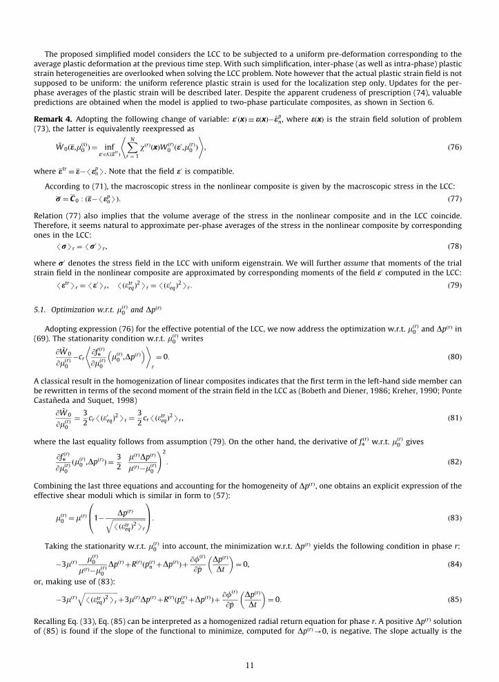
The proposed simplified model considers the LCC to be subjected to a uniform pre-deformation corresponding to theaverage plastic deformation at the previous time step. With such simplification, inter-phase (as well as intra-phase) plasticstrain heterogeneities are overlooked when solving the LCC problem. Note however that the actual plastic strain field is notsupposed to be uniform: the uniform reference plastic strain is used for the localization step only. Updates for the per-phase averages of the plastic strain will be described later. Despite the apparent crudeness of prescription (74), valuablepredictions are obtained when the model is applied to two-phase particulate composites, as shown in Section 6.

Remark 4. Adopting the following change of variable: e0ðxÞ & eðxÞ'epn, where eðxÞ is the strain field solution of problem(73), the latter is equivalently reexpressed as

~W 0ðe,mðsÞ0 Þ ¼ inf

e02Kðe tr Þ

XN

r ¼ 1

wðrÞðxÞW ðrÞ0 ðe0,mðrÞ

0 Þ

* +, ð76Þ

where etr & e'/epnS. Note that the field e0 is compatible.

According to (71), the macroscopic stress in the nonlinear composite is given by the macroscopic stress in the LCC:

r ¼ C 0 : ðe'/epnSÞ: ð77Þ

Relation (77) also implies that the volume average of the stress in the nonlinear composite and in the LCC coincide.Therefore, it seems natural to approximate per-phase averages of the stress in the nonlinear composite by correspondingones in the LCC:

/rSr ¼/r0Sr , ð78Þ

where r0 denotes the stress field in the LCC with uniform eigenstrain. We will further assume that moments of the trialstrain field in the nonlinear composite are approximated by corresponding moments of the field e0 computed in the LCC:

/etrSr ¼/e0Sr , /ðetreqÞ2Sr ¼/ðe0eqÞ2Sr : ð79Þ

5.1. Optimization w.r.t. mðrÞ0 and DpðrÞ

Adopting expression (76) for the effective potential of the LCC, we now address the optimization w.r.t. mðrÞ0 and DpðrÞ in

(69). The stationarity condition w.r.t. mðrÞ0 writes

@ ~W 0

@mðrÞ0

'cr@f ðrÞn

@mðrÞ0

mðrÞ0 ,DpðrÞ

( )* +

r

¼ 0: ð80Þ

A classical result in the homogenization of linear composites indicates that the first term in the left-hand side member canbe rewritten in terms of the second moment of the strain field in the LCC as (Bobeth and Diener, 1986; Kreher, 1990; PonteCastaneda and Suquet, 1998)

@ ~W 0

@mðrÞ0

¼32cr/ðe0eqÞ2Sr ¼

32cr/ðetreqÞ2Sr , ð81Þ

where the last equality follows from assumption (79). On the other hand, the derivative of f ðrÞn w.r.t. mðrÞ0 gives

@f ðrÞn

@mðrÞ0

ðmðrÞ0 ,DpðrÞÞ ¼

32

mðrÞDpðrÞ

mðrÞ'mðrÞ0

!2

: ð82Þ

Combining the last three equations and accounting for the homogeneity of DpðrÞ, one obtains an explicit expression of theeffective shear moduli which is similar in form to (57):

mðrÞ0 ¼ mðrÞ 1'

DpðrÞffiffiffiffiffiffiffiffiffiffiffiffiffiffiffiffiffiffiffiffiffi/ðetreqÞ2Sr

q

0

B@

1

CA: ð83Þ

Taking the stationarity w.r.t. mðrÞ0 into account, the minimization w.r.t. DpðrÞ yields the following condition in phase r:

'3mðrÞ mðrÞ0

mðrÞ'mðrÞ0

DpðrÞ þRðrÞðpðrÞn þDpðrÞÞþ@fðrÞ

@ _pDpðrÞ

Dt

! "¼ 0, ð84Þ

or, making use of (83):

'3mðrÞffiffiffiffiffiffiffiffiffiffiffiffiffiffiffiffiffiffiffiffiffi/ðetreqÞ2Sr

qþ3mðrÞDpðrÞ þRðrÞðpðrÞn þDpðrÞÞþ

@fðrÞ

@ _pDpðrÞ

Dt

! "¼ 0: ð85Þ

Recalling Eq. (33), Eq. (85) can be interpreted as a homogenized radial return equation for phase r. A positive DpðrÞ solutionof (85) is found if the slope of the functional to minimize, computed for DpðrÞ-0, is negative. The slope actually is the

11

left-hand side of (85). The unique yield criterion for phase r reads

'3mðrÞffiffiffiffiffiffiffiffiffiffiffiffiffiffiffiffiffiffiffiffiffi/ðetreqÞ2Sr

qþRðrÞðpðrÞn ÞþsðrÞ

Y o0: ð86Þ

In the yield criterion (86) the second moment /ðetreqÞ2Sr is computed on the LCC characterized by the elastic shear modulimðrÞ. Indeed, mðrÞ

0 -mðrÞ as DpðrÞ-0, according to expression (83). If the yield criterion (86) is not satisfied, the increment iselastic in phase r, and the minimum is achieved for DpðrÞ ¼ 0. Otherwise, the radial return condition (85) takes the familiarform (35):

'3mðrÞffiffiffiffiffiffiffiffiffiffiffiffiffiffiffiffiffiffiffiffiffi/ðetreqÞ2Sr

qþ3mðrÞDpðrÞ þRðrÞðpðrÞn þDpðrÞÞþsðrÞ

Y ¼ 0: ð87Þ

Since Eq. (87) may be rewritten asffiffiffiffiffiffiffiffiffiffiffiffiffiffiffiffiffiffiffiffiffi/ðetreqÞ2Sr

q¼DpðrÞ þ

13mðrÞ ðR

ðrÞðpðrÞn þDpðrÞÞþsðrÞY Þ, ð88Þ

the second term of the right hand side is always positive. Hence,ffiffiffiffiffiffiffiffiffiffiffiffiffiffiffiffiffiffiffiffiffi/ðetreqÞ2Sr

q4DpðrÞ and mðrÞ

0 is always positive, asannounced.

5.2. Homogenized flow rule

The proposed estimate of the composite mechanical response also requires computation of the phase average of theplastic strain (or plastic strain increment) at each time step:

/DepS¼XN

r ¼ 1

cr/DepSr ¼XN

r ¼ 1

crDpðrÞetr

etreq

* +

r

: ð89Þ

The average plastic strain update is computed by making use of the following observations. On the one hand, the phaseaverage of the stress is given by

/rSr ¼ CeðrÞ : /etr'DepSr ¼ CeðrÞ : /etrSr'2mðrÞ/DepSr : ð90Þ

On the other hand, according to (78), we also have

/rSr ¼/r0Sr ¼ CðrÞ0 : /e0Sr ¼ CeðrÞ : /e0Sr'2mðrÞDpðrÞ

/e0Srffiffiffiffiffiffiffiffiffiffiffiffiffiffiffiffiffiffiffiffiffi/ðe0eqÞ2Sr

q : ð91Þ

The last equality is obtained using expression (83) of the shear modulus mðrÞ0 . Making use of assumption (79), a direct

comparison of the last two expressions yields

/DepSr ¼DpðrÞetr

etreq

* +

r

¼DpðrÞ/etrSrffiffiffiffiffiffiffiffiffiffiffiffiffiffiffiffiffiffiffiffiffi/ðetreqÞ2Sr

q , ð92Þ

which defines an effective flow direction NðrÞ for phase r:

NðrÞ &/etrSrffiffiffiffiffiffiffiffiffiffiffiffiffiffiffiffiffiffiffiffiffi/ðetreqÞ2Sr

q : ð93Þ

Eq. (92) can be viewed as a homogenized plastic flow rule for the average plastic strain.

Remark 5. In general, NðrÞ : NðrÞa3=2. Instead:

NðrÞ : NðrÞ ¼32

ð/etrSrÞ2eq

/ðetreqÞ2Sr

, ð94Þ

where the second-order moment of etr is necessarily greater than the first-order moment, except in very specific situationswhere fields are homogeneous in each phase.

5.3. Summary of the homogenization procedure

Taking advantage of formulation (76) for the effective behavior of the LCC, algorithmic implementation is ratherstraightforward. We consider a composite in a strain- and stress-free configuration at t¼t0. On a time interval ½tn,tnþ1), historyvariables at tn are given for each phase r: /epnSr and /pnSr . Given e, the macroscopic strain at tnþ1, the problem is to computethe macroscopic stress r. In the proposed numerical procedure, we iterate on the value of the reference shear moduli mðrÞ

0 .

- Elastic predictor step. Taking mðrÞ0 ¼ mðrÞ:

1. Compute the effective stiffness C 0 according to the chosen homogenization scheme for a linear elastic composite.Next, compute /ðetreqÞ2Sr according to Eq. (81).

12

2. Evaluate the yield criterion (86) in each phase:

kðrÞðrÞ &'3mðrÞffiffiffiffiffiffiffiffiffiffiffiffiffiffiffiffiffiffiffiffiffi/ðetreqÞ2Sr

qþRðrÞðpðrÞn ÞþsðrÞ

Y :

3. If kðrÞZ0: the increment is elastic in phase r, and mðrÞ0 ¼ mðrÞ and DpðrÞ ¼ 0.

4. Otherwise, mðrÞ0 is smaller than mðrÞ and it must be found iteratively.

- Plastic correction step. Iteration (i) (upper index (i) omitted for simplicity). Compute the effective stiffness C 0 accordingto the chosen homogenization scheme for a linear elastic composite. For each phase r in which plastic yielding occurs:1. Compute /ðetreqÞ2Sr according to Eq. (81).2. Compute DpðrÞ according to Eq. (83):

DpðrÞ ¼mðrÞ'mðrÞ

0

mðrÞ

ffiffiffiffiffiffiffiffiffiffiffiffiffiffiffiffiffiffiffiffiffi/ðetreqÞ2Sr

q:

3. Compute the residual (radial return Eq. (87)):

FðrÞ & '3mðrÞffiffiffiffiffiffiffiffiffiffiffiffiffiffiffiffiffiffiffiffiffi/ðetreqÞ2Sr

qþ3mðrÞDpðrÞ þRðrÞðpðrÞn þDpðrÞÞþsðrÞ

Y :

Iterate on mðrÞ0 until the absolute value of the residual in each phase becomes lower than a given tolerance.

- After convergence. Compute the increment of average plastic strain:

/DepSr ¼DpðrÞ/etrSrffiffiffiffiffiffiffiffiffiffiffiffiffiffiffiffiffiffiffiffiffi/ðetreqÞ2Sr

q ,

and update the internal variables:

/epSr ¼/epnSrþ/DepSr ,

pðrÞ ¼ pðrÞn þDpðrÞ:

Finally, the macroscopic stress is obtained from the effective stiffness of the LCC as

r ¼ C 0 : ðe'/epnSÞ ¼/rS:

In cases where an expression for the effective stiffness C0 is available in closed form, the procedure is implemented usingthe Newton–Raphson method. In the examples of the next section, three iterations are typically sufficient to reachconvergence.

6. Application to two particle-reinforced composites

In this section we compare the predictions of the simplified model proposed in Section 5 to reference results obtainedfrom full-field finite element (FE) simulations for several two-phase composites. We consider composites made of a squarearray of spherical inclusions, which are frequently approximated by axisymmetric unit cells (Fig. 3(a)) allowing full-fieldcomputations at low cost. The geometry is meshed using the GMSH software (Geuzaine and Remacle, 2009), and a typicalmesh comprises approximately 1000 elements and 2700 nodes (Fig. 3(b)). A convergence study was successfullyconducted by comparing the predictions to those obtained with finer meshes (about 2500 elements). FE computationsare performed using ABAQUS 6.9 (2009) using quadratic CAX6 and CAX8 elements. Reference, FE predictions are labeled‘‘FE’’ in the figures.

Regarding the simplified model, two approaches have been pursued to solve the localization problem over the LCC. Onthe one hand, the LCC is homogenized ‘‘exactly’’ using the FE method. In this case, first- and second-order moments ofstress and strain fields involved in the procedure are computed from direct volume averaging of the local fields in the LCC.

Fig. 3. (a) Reference predictions for composites with periodic microstructure are obtained considering cylindrical unit cells. (b) FE computations areperformed using axisymmetric elements.

13

In this way, the linearization procedure, together with the other approximation introduced in Section 5, are assessed whileavoiding additional errors related to the use of an approximate linear homogenization scheme. This methodology wasalready used in order to evaluate the capabilities of linearization methods by Rekik et al. (2007) and Lahellec and Suquet(2007a). Corresponding results are labeled ‘‘VARþFE’’ in the figures.

Alternatively, (hopefully) reliable estimates of the effective response of inclusion-reinforced linear elastic compositesare provided by Hashin–Shtrikman (HS) lower bound (Hashin and Shtrikman, 1963; Willis, 1977). An advantage of the HSbounds is the relative simplicity of implementation: an expression of the effective stiffness of the LCC is then available inclosed-form. The predictions of the variational method combined with the HS lower bound are labeled ‘‘VARþHS-’’ in thefigures.

The composites are subjected to uniaxial tension in the z-direction. The boundary conditions applied to the unit cell arethe following:

u3ðr,z¼H=2Þ ¼ u3, 0oroR,

u3ðr,z¼ 0Þ ¼ 0, 0oroR,

u1ðr¼ 0,zÞ ¼ 0, 0ozoH=2,

u1ðr¼ R,zÞ ¼ u1, 0ozoH=2,

with H¼2R. The displacement u3 is prescribed, while u1 is a priori unknown as the r¼R boundary is traction-free. Loadinginvolves 50 time increments unless otherwise indicated.

6.1. Elastic inclusions, elasto-plastic matrix

The material under consideration is a metal matrix composite (MMC) with the following properties:

- Inclusions (phase 1): E¼400 GPa, n¼ 0:2.- Matrix (phase 2): E¼75 GPa, n¼ 0:3, sY ¼ 75 MPa, RðpÞ ¼ hpn, h¼400 MPa, n¼0.4 or n¼0.05.

Two volume fractions of inclusions are considered: c1¼0.15 and c1¼0.30. MMC’s with similar material properties werepreviously considered by several authors aiming to assess homogenization models (Segurado et al., 2002; Michel andSuquet, 2003; Doghri and Ouaar, 2003; Gonzalez et al., 2004; Chaboche et al., 2005; Pierard et al., 2007) so that thepredictive capabilities of the present approach can easily be evaluated w.r.t. those schemes.

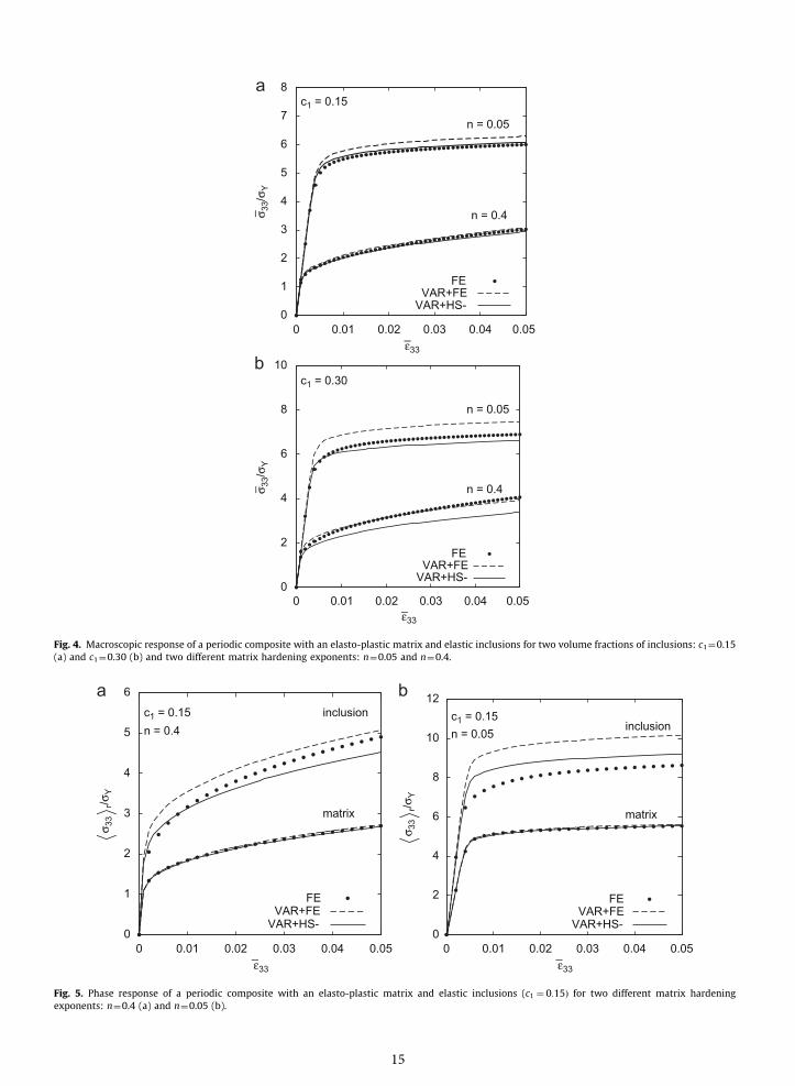
The effective response for both hardening exponents and volume fractions is presented in Fig. 4. The VARþFE modelgives satisfying predictions for both volume fractions in the case n¼0.4, while it overestimates the reference responsewhen n¼0.05. In the latter case, better predictions are obtained using HS lower bound to homogenize the LCC (VARþHS-model), due to the compensation of errors between the underestimation brought by the HS lower bound and theoverestimation due to the present choice of LCC. On the other hand, the prediction of the VARþHS-model are too soft inthe case c1¼0.30 and n¼0.4.

The accuracy of the model regarding the phase response is assessed in Fig. 5 taking c1¼0.15. For both hardeningexponents, the proposed estimate correctly predicts the matrix response, even without the additional underestimationbrought by the HS model. The evolution of the accumulated plastic strain in the matrix is also very well captured by thehomogenization models (not shown). The method is less accurate regarding the inclusion response. There is a largediscrepancy between VARþFE and VARþHS-results observed in the inclusions, while they are remarkably close in thematrix.

Previous examples showed that the model is less accurate when the matrix presents weak hardening. A limit case isobtained considering a perfectly plastic matrix: R(p)¼0 (other material properties left unchanged). As expected fromprevious observations, the VARþFE model overestimates the effective response (Fig. 6(a)), due to an unsuccessfulprediction of the inclusion response (Fig. 6(b)). Predictions are more accurate using HS lower bound to homogenizethe LCC.

Convergence of the model is analyzed in Fig. 7 for c1¼0.15 and n¼0.4, by successively considering 20, 50 and 100increments to achieve the total elongation. It has been checked against results obtained using a very large number ofincrements (up to 10 000) that the curve with 100 increments can be considered as a converged result. The scatterbetween the stress–strain curves presented in the figure is very low, as required. Obviously, sufficiently small loading stepsare needed to capture the elastic–plastic transition accurately. Similar conclusions hold for n¼0.05 and the case of aperfectly plastic matrix.

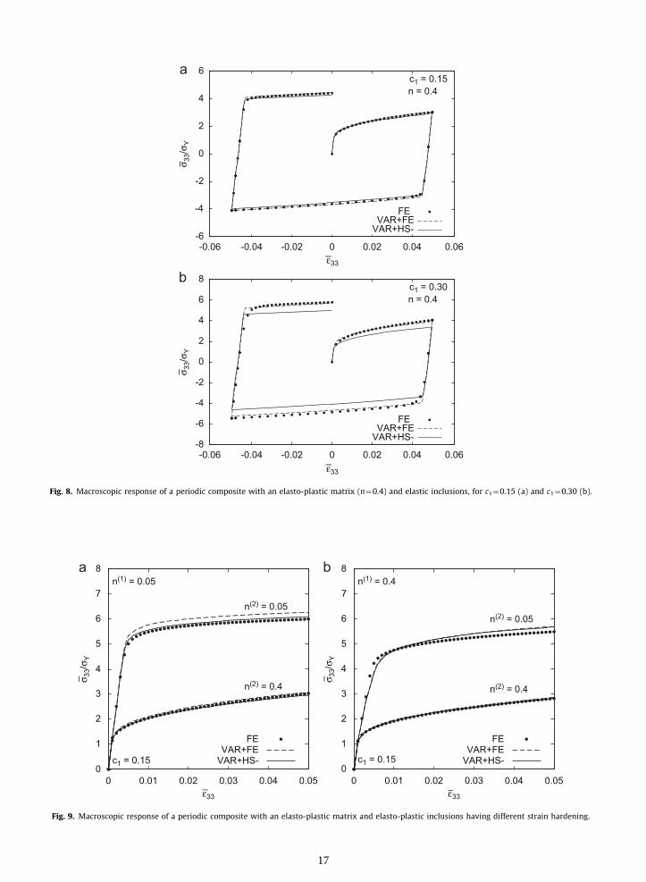
The variational procedure is able to simulate non-monotonic loadings. Examples of uniaxial tension/compression testsfor c1¼0.15 and c1¼0.30 are presented in Fig. 8, taking n¼0.4. The figure shows comparable accuracy of the proposedmodels in tension and compression. For c1¼0.30, the full-field simulation demonstrates a Baushinger effect (early andprogressive plastification in the unloading branches of the cycle). Such effect is related to the heterogeneity of the plasticstrain field which developed during the initial step of uniaxial tension. The proposed model predicts a sharp elastic–plastic

14

0

1

2

3

4

5

6

7

8

0 0.01 0.02 0.03 0.04 0.05

σ 33/σ

Y

ε33

n = 0.05

n = 0.4

c1 = 0.15

FEVAR+FE

VAR+HS-

0

2

4

6

8

10

0 0.01 0.02 0.03 0.04 0.05

σ 33/σ

Y

ε33

n = 0.05

n = 0.4

c1 = 0.30

FEVAR+FE

VAR+HS-

Fig. 4. Macroscopic response of a periodic composite with an elasto-plastic matrix and elastic inclusions for two volume fractions of inclusions: c1¼0.15(a) and c1¼0.30 (b) and two different matrix hardening exponents: n¼0.05 and n¼0.4.

0

1

2

3

4

5

6

0 0.01 0.02 0.03 0.04 0.05ε33 ε33

inclusion

matrix

c1 = 0.15n = 0.4

FEVAR+FE

VAR+HS-0

2

4

6

8

10

12

0 0.01 0.02 0.03 0.04 0.05

σ 33

r/σY

σ 33

r/σY

inclusion

matrix

c1 = 0.15n = 0.05

FEVAR+FE

VAR+HS-

Fig. 5. Phase response of a periodic composite with an elasto-plastic matrix and elastic inclusions (c1 ¼ 0:15Þ for two different matrix hardeningexponents: n¼0.4 (a) and n¼0.05 (b).

15

transition in compression, as the homogenized yield criterion (86) for the matrix phase accounts for isotropic hardeningonly. Nevertheless, the stress level after the effective elastic–plastic transition is correctly predicted by the VARþFE model.

6.2. Elasto-plastic inclusions, elasto-plastic matrix

We continue with a composite made of two elasto-plastic phases:

- Inclusions (phase 1): E¼400 GPa, n¼ 0:2, sY ¼ 75 MPa, Rð1ÞðpÞ ¼ hð1Þpnð1Þ, hð1Þ ¼ 1 GPa, nð1Þ ¼ 0:4 or nð1Þ ¼ 0:05.

- Matrix (phase 2): E¼75 GPa, n¼ 0:3, sY ¼ 75 MPa, Rð2ÞðpÞ ¼ hð2Þpnð2Þ, hð2Þ ¼ 400 MPa, nð2Þ ¼ 0:4 or nð2Þ ¼ 0:05.

The volume fraction of inclusions is c1¼0.15.The effective response of the composite is presented in Fig. 9 for all combinations of inclusion and matrix hardening

exponents. The responses for nð1Þ ¼ 0:05 in Fig. 9(a) are very close to those presented in Fig. 4(a) for composites reinforcedby elastic inclusions. Indeed, it can be checked that plastic deformations in the inclusions are negligible (although non-zero). On the contrary, when nð1Þ ¼ 0:4 (Fig. 9(b)), plastic deformations are important in both phases. Interestingly, theVARþFE and VARþHS-models predict almost identical effective response, whereas this is not necessarily true at thephase level.

0

0.2

0.4

0.6

0.8

1

1.2σ 3

3/σY

c1 = 0.15

FEVAR+FE

VAR+HS-0

0.5

1

1.5

2

0 0.001 0.002 0.003 0.004 0.005 0 0.001 0.002 0.003 0.004 0.005

σ 33

r/σY

ε33ε33

inclusion

matrix

c1 = 0.15

FEVAR+FE

VAR+HS-

Fig. 6. Macroscopic (a) and phase (b) response of a periodic composite with a perfectly plastic matrix (RðpÞ ¼ 0) and elastic inclusions (c1¼0.15).

0

0.5

1

1.5

2

2.5

3

0 0.01 0.02 0.03 0.04 0.05

σ 33/σ

Y

ε33

c1 = 0.15n = 0.4

VAR+HS-,∆ε33 = 2.5 × 10−3

∆ε33 = 1 × 10−3

∆ε33 = 5 × 10−4

Fig. 7. Macroscopic response of a periodic composite with an elasto-plastic matrix (n¼0.4) and elastic inclusions (c1 ¼ 0:15Þ as predicted by theVARþHS-model, successively taking 20, 50 and 100 strain increments to reach the final elongation.

16

-6

-4

-2

0

2

4

6

σ 33/σ

Y

ε33

c1 = 0.15n = 0.4

FEVAR+FE

VAR+HS-

-8

-6

-4

-2

0

2

4

6

8

-0.06 -0.04 -0.02 0 0.02 0.04 0.06

-0.06 -0.04 -0.02 0 0.02 0.04 0.06

σ 33/σ

Y

ε33

c1 = 0.30n = 0.4

FEVAR+FE

VAR+HS-

Fig. 8. Macroscopic response of a periodic composite with an elasto-plastic matrix (n¼0.4) and elastic inclusions, for c1¼0.15 (a) and c1¼0.30 (b).

0

1

2

3

4

5

6

7

8

0 0.01 0.02 0.03 0.04 0.05

σ 33/σ

Y

ε33

n(2) = 0.05

n(2) = 0.4

c1 = 0.15

n(1) = 0.05

FEVAR+FE

VAR+HS-0

1

2

3

4

5

6

7

8

0 0.01 0.02 0.03 0.04 0.05

σ 33/σ

Y

ε33

n(2) = 0.05

n(2) = 0.4

c1 = 0.15

n(1) = 0.4

FEVAR+FE

VAR+HS-

Fig. 9. Macroscopic response of a periodic composite with an elasto-plastic matrix and elasto-plastic inclusions having different strain hardening.

17

6.3. Perfectly plastic inclusions and matrix

Finally, we consider the case of two perfectly plastic phases: Rð1ÞðpÞ ¼ Rð2ÞðpÞ ¼ 0 with identical yield stresses but distinctelastic properties, identical to those considered before. The overall yield stress of the composite is obviouslysY ¼ sð1Þ

Y ¼ sð2ÞY , and the heterogeneous elastic properties should affect only the macroscopic yield strain. Unfortunately,

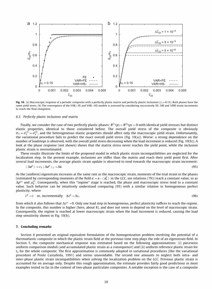
the variational procedure fails to predict the exact overall yield stress (Fig. 10(a)). Worse: a strong dependence on thenumber of loadsteps is observed, with the overall yield stress decreasing when the load increment is reduced (Fig. 10(b)). Alook at the phase response (not shown) shows that the matrix stress never reaches the yield point, while the inclusionplastic strain is overestimated.

These results illustrate the limits of the proposed model in which plastic strain incompatibilities are neglected for thelocalization step. In the present example, inclusions are stiffer than the matrix and reach their yield point first. Afterseveral load increments, the average plastic strain update is observed to tend towards the macroscopic strain increment:

/DepS¼ c1/DepS1-De: ð95Þ

As the (uniform) eigenstrain increases at the same rate as the macroscopic strain, moments of the trial strain in the phases(estimated by corresponding moments of the field e0 ¼ e'/epnS in the LCC, see relations (79)) reach a constant value, so asDpðrÞ and mðrÞ

0 . Consequently, when this ‘‘regime’’ stage is reached, the phase and macroscopic stress tend to a constantvalue. Such behavior can be intuitively understood comparing (95) with a similar relation in homogeneous perfectplasticity, where

_ep-_e or, incrementally Dep-De, ð96Þ

from which it also follows that Detr-0. Only one load step in homogeneous, perfect plasticity suffices to reach the regime.In the composite, this number is higher (here, about 8), and does not seem to depend on the level of macroscopic strain.Consequently, the regime is reached at lower macroscopic strain when the load increment is reduced, causing the loadstep sensitivity shown in Fig. 10(b).

7. Concluding remarks

Section 4 presented an original equivalent formulation of the homogenization problem involving the potential of athermoelastic composite in which the plastic strain field at the previous time step plays the role of an eigenstrain field. InSection 5, the composite mechanical response was estimated based on the following approximations: (i) piecewiseuniform comparison moduli (and accumulated plastic strain as a consequence) and (ii) uniform reference plastic strain fortn for the whole composite. The first approximation is commonly adopted in variational procedures (like the variationalprocedure of Ponte Castaneda, 1991) and seems unavoidable. The second one amounts to neglect both intra- andinter-phase plastic strain incompatibilities when solving the localization problem on the LCC. Previous plastic strain isaccounted for on average only. Despite this rough approximation, the estimate provides fairly good predictions in mostexamples tested so far in the context of two-phase particulate composites. A notable exception is the case of a composite

0

0.2

0.4

0.6

0.8

1

1.2σ 3

3/σY

ε33

c1 = 0.15

FEVAR+FE

VAR+HS-0

0.2

0.4

0.6

0.8

1

1.2

0 0.001 0.002 0.003 0.004 0.005 0 0.001 0.002 0.003 0.004 0.005

σ 33/σ

Y

ε33

∆ ε33 = 1 × 10−4

∆ ε33 = 5 × 10−5

∆ ε33 = 5 × 10−6

c1 = 0.15VAR+FE

VAR+HS-

Fig. 10. (a) Macroscopic response of a periodic composite with a perfectly plastic matrix and perfectly plastic inclusions (c1¼0.15). Both phases have thesame yield stress. (b) The convergence of the VARþFE and VARþHS-models is assessed by considering successively 50, 100 and 1000 strain incrementsto reach the final elongation.

18

with two perfectly plastic phases having the same yield stress (Section 6.3). In this case, neglecting inter-phase plasticincompatibilities leads to inconsistent results.

Important aspects of the proposed method are summarized:

- The model is designed for true elasto-plasticity, and does not require the approximation of visco-plasticity or perfectplasticity. One explicitly accounts for the existence of an elasticity domain, nonlinear hardening, and the hereditarybehavior. In particular, arbitrary loading paths are handled.

- The formulation suggests an original localization rule for elasto-plastic composites based on ‘‘trial secant’’ operatorscomputed for the second moments of the trial strain field. These operators are softer than the correspondingelastic ones.

- The algorithmic structure of the incremental equations of elasto-plasticity is preserved in the homogenization scheme.The model yields a homogenized yield criterion for each elasto-plastic phase, and a homogenized radial return equationfor the internal variable. Both the homogenized yield criterion and the return mapping equation are based on thesecond-order moment of the trial strain field as a result from the variational procedure. A homogenized flow rule forper-phase averages of the plastic strain was also derived.

Future developments of the approach should focus on the account of inter-phase plastic strain incompatibilities in thelocalization problem. This can be achieved considering piecewise uniform reference plastic strain in the thermoelasticproblem (70), instead of a uniform one. However, the definition of a proper uniform reference plastic strain for the phase isnot straightforward (Lahellec and Suquet, 2007a; Brassart, 2011), and is left for future work.

Acknowledgments

L.B. and L.D. are mandated by the National Fund for Scientific Research (FNRS, Belgium). The authors thank the reviewerfor a very constructive review which pointed out shortcomings in the initial manuscript, and N. Lahellec for helpfuldiscussions.

Appendix A. Computation of the kinematic variable using Lagrange multipliers

The kinematic variable N must minimize the functional JD (23) under constraints (6). The corresponding Lagrangianfunctional reads

Lðenþ1,pnþ1,N,l1,l2Þ ¼12ðetrnþ1'DpNÞ : Ce : ðetrnþ1'DpNÞþcpðpnþ1Þ'cnþDtf Dp

Dt

! "þl1 trðNÞþl2 N : N'

32

! ":

ð97Þ

The kinematic variable N must satisfy the following condition:@L@N

ðenþ1,pnþ1,N,l1,l2Þ ¼ 0, ð98Þ

that is,

0¼'DpCe : ðetrnþ1'DpNÞþl11þ2l2N ¼'Dpðrtrnþ1'DpðC

e : NÞÞþl11þ2l2N: ð99Þ

Additional hypotheses about the free-energy function are required in order to determine N. Here, isotropic elasticity isassumed, so that the elastic stiffness tensor may be decomposed into volumetric and deviatoric parts, see expression (32).In this case, condition (99) becomes

'Dp rtrnþ1'2mDpN

* +þl11þ2l2N ¼ 0: ð100Þ

The trace of the above expression is computed, leading to

l1 ¼ 13Dp trðrtr

nþ1Þ, ð101Þ

which, introduced in (100) yields

'Dpðrtrnþ1'

13 trðr

trnþ1ÞÞ1þ2mðDpÞ2Nþ2l2N ¼ 0, ð102Þ

which can be rewritten as

'Dpðstrnþ1Þ ¼'2mðDpÞ2N'2l2N: ð103Þ

This equation shows that the direction N is ‘‘aligned’’ with the tensor strnþ1. The normalizing condition in (6) finally gives

N ¼32

strnþ1

streq,nþ1

: ð104Þ

19

Appendix B. Link with the transformation field analysis (TFA)

A straightforward simplification to problem (50) would be to restrict the space of solutions for the internal andkinematic variables to piecewise uniform fields:

DpðxÞ ¼XN

r ¼ 1

wðrÞðxÞDpðrÞ, NðxÞ ¼XN

r ¼ 1

wðrÞðxÞNðrÞ, ð105Þ

with trðNðrÞÞ ¼ 0 and NðrÞ : NðrÞ ¼ 3=2. Consequently, the plastic strain tensor is also piecewise uniform:

epðxÞ ¼XN

r ¼ 1

wðrÞðxÞepðrÞ, ð106Þ

its update being given by the following discretized flow rule:

DepðrÞ ¼DpðrÞNðrÞ: ð107Þ

Using the trial fields (105) in (50) leads to an upper bound for the effective incremental potential (indices nþ1 are omittedfor simplicity):

WDðeÞr infe2KðeÞ

infDpðsÞ ,NðsÞ

XN

r ¼ 1

wðrÞðxÞ cðrÞðe,epðrÞ,pðrÞÞ'cðrÞn ðxÞþDtfðrÞ DpðrÞ

Dt

! "% &( )* +: ð108Þ

Permuting the order of the infimum operations over the strain field and the internal variables, the following alternativeexpression is obtained:

WDðeÞr infDpðsÞ ,NðsÞ

W 0ðe,epðsÞÞþXN

r ¼ 1

wðrÞðxÞ cpðrÞðpðrÞÞ'cðrÞn ðxÞþDtfðrÞ DpðrÞ

Dt

! "! "* +( )

, ð109Þ

where

W 0ðe,epðsÞÞ ¼ infe2KðeÞ

XN

r ¼ 1

wðrÞðxÞ12ðe'epðrÞÞ : Ce : ðe'epðrÞÞ

* +: ð110Þ

Consequently, the local stress and strain fields may be determined from an elastic analysis on a thermoelastic composite inwhich the piecewise uniform plastic strain acts as an eigenstrain. This is exactly the assumption sustaining the TFA.

The stationarity condition w.r.t. DpðrÞ in (109) yields the condition:

/YðNðrÞ,pðrÞÞSr ¼/rSr : NðrÞ'RðrÞðpðrÞÞ ¼

@fðrÞ

@ _pDpDt

! "* +

r

: ð111Þ

The constrained minimization w.r.t. NðrÞ is performed using Lagrange multipliers (see Appendix A), leading to

NðrÞ ¼/e'epðrÞn Sr

ð/e'epðrÞn SrÞeq: ð112Þ

Combining the last two equations, it is readily seen that DpðrÞ obeys the radial return scheme driven by the first moment ofthe stress in phase r of the thermoelastic composite.

References

ABAQUS 6.9, 2009. A General-purpose Finite Element Software. ABAQUS Inc., Pawtucket, RI, USA.Benveniste, Y., 1987. A new approach to the application of Mori–Tanaka’s theory in composite materials. Mech. Mater. 6, 147–157.Berveiller, M., Zaoui, A., 1979. An extension of the self-consistent scheme to plastically-flowing polycrystals. J. Mech. Phys. Solids 26, 325–344.Bobeth, M., Diener, G., 1986. Field fluctuations in multicomponent mixtures. J. Mech. Phys. Solids 34, 1–17.Brassart, L., 2011. Homogenization of Elasto-(visco)plastic Composites: History-dependent Incremental and Variational Approaches. Ph.D. Thesis, Ecole

Polytechnique de Louvain, Universite catholique de Louvain. URL /http://dial.academielouvain.be/handle/boreal:75974S.Buryachenko, V., 1999. Elastic–plastic behavior of elastically homogeneous materials with a random field of inclusions. Int. J. Plasticity 15, 687–720.Carini, A., 1996. Colonnetti’s minimum principle extension to generally non-linear materials. Int. J. Solids Struct. 33, 121–144.Chaboche, J.-L., Kanoute, P., 2003. Sur les approximations ‘‘isotrope’’ et ‘‘anisotrope’’ de l’operateur tangent pour les methodes tangentes incrementale et

affine. C. R. Mecanique 331, 857–864.Chaboche, J.L., Kanoute, P., Roos, A., 2005. On the capabilities of mean-field approaches for the description of plasticity in metal matrix composites. Int. J.

Plasticity 21, 1409–1434.Chaboche, J.-L., Kruch, S., Maire, J., Pottier, T., 2001. Towards a micromechanics based inelastic and damage modeling of composites. Int. J. Plasticity 17,

411–439.Comi, C., Corigliano, A., Maier, G., 1991. Extremum properties of finite-step solutions in elastoplasticity with nonlinear hardening. Int. J. Solids Struct. 27,

965–981.Doghri, I., 2000. Mechanics of Deformable Solids: Linear and Nonlinear, Analytical and Computational Aspects. Springer.Doghri, I., Friebel, C., 2005. Effective elasto-plastic properties of inclusion-reinforced composites. Study of shape, orientation and cyclic response. Mech.

Mater. 37, 45–68.Doghri, I., Ouaar, A., 2003. Homogenization of two-phase elasto-plastic composite materials and structures: study of tangent operators, cyclic plasticity

and numerical algorithms. Int. J. Solids Struct. 40, 1681–1712.

20

Dvorak, G., 1992. Transformation field analysis of inelastic composite materials. Proc. R. Soc. London A 437, 311–327.Dvorak, G., Benveniste, Y., 1992. On transformation strains and uniform fields in multiphase elastic media. Proc. R. Soc. London A 437, 291–310.Germain, P., Nguyen, Q., Suquet, P., 1983. Continuum thermodynamics. J. Appl. Mech. 50, 1010–1020.Geuzaine, C., Remacle, J.-F., 2009. Gmsh: a three-dimensional finite element mesh generator with built-in pre- and post-processing facilities. Int. J.

Numer. Meth. Eng. 79, 1309–1331.Gilormini, P., 1995. Insuffisance de l’extension classique du mod!ele auto-coherent au comportement non lineaire. C. R. Acad. Sci. Paris 320 (Serie IIb),

115–122.Gonzalez, C., LLorca, J., 2000. A self-consistent approach to the elasto-plastic behaviour of two-phase materials including damage. J. Mech. Phys. Solids 48,

675–692.Gonzalez, C., Segurado, J., LLorca, J., 2004. Numerical simulation of elasto-plastic deformation of composites: evolution of stress microfields and

implications for homogenization models. J. Mech. Phys. Solids 52, 1573–1593.Halphen, B., Nguyen, Q., 1975. Sur les materiaux standards generalises. J. Mec. 14, 39–63.Hashin, Z., Shtrikman, S., 1963. A variational approach to the theory of the elastic behavior of multiphase materials. J. Mech. Phys. Solids 11, 127–140.Hill, R., 1965a. Continuum micro-mechanics of elastoplastic polycrystals. J. Mech. Phys. Solids 13, 89–101.Hill, R., 1965b. A self-consistent mechanics of composite materials. J. Mech. Phys. Solids 13, 213–222.Hill, R., 1967. The essential structure of constitutive laws for metal composites and polycrystals. J. Mech. Phys. Solids 15, 79–95.Hutchinson, J.W., 1970. Elastic–plastic behaviour of polycrystalline metals and composites. Proc. R. Soc. London A 319, 247–272.Hutchinson, J.W., 1976. Bounds and self-consistent estimates for creep of polycrystalline materials. Proc. R. Soc. London A 348, 101–127.Kreher, W.S., 1990. Residual stresses and stored elastic energy of composites and polycrystals. J. Mech. Phys. Solids 38, 115–128.Kroner, E., 1958. Berechnung der elastischen konstanten des vielkristalls aus den konstanten des einkristalls. Z. Phys. 151, 504–518.Lahellec, N., Suquet, P., 2007a. On the effective behavior of nonlinear inelastic composites: I. Incremental variational principles. J. Mech. Phys. Solids 55,

1932–1963.Lahellec, N., Suquet, P., 2007b. On the effective behavior of nonlinear inelastic composites: II. A second-order procedure. J. Mech. Phys. Solids 55,

1964–1992.Lebensohn, R., Tome, C., 1993. A self-consistent anisotropic approach for the simulation of plastic deformation and texture development of polycrystals:

application to zirconium alloys. Acta Metall. Mater. 41, 2611–2624.Lemaıtre, J., Chaboche, J.-L., 1990. Mechanics of Solid Materials. Cambridge University Press.Martin, J.B., Kaunda, M.A.E., Isted, R., 1996. Internal variable formulations of elastic–plastic dynamic problems. Int. J. Impact Eng. 18, 849–858.Masson, R., Bornert, M., Suquet, P., Zaoui, A., 2000. An affine formulation for the prediction of the effective properties of nonlinear composites and

polycrystals. J. Mech. Phys. Solids 48, 1203–1227.Maugin, G.A., 1992. The Thermomechanics of Plasticity and Fracture. Cambridge University Press.Mialon, P., 1986. Elements d’analyse et de resolution numerique des relations de l’elasto-plasticite. EDF Bull. Dir. Etud. Rech. Ser. C 3, 57–89.Michel, J., Suquet, P., 2003. Nonuniform transformation field analysis. Int. J. Solids Struct. 40, 6937–6955.Miehe, C., 2002. Strain-driven homogenization of inelastic microstructures and composites based on an incremental variational formulation. Int. J.

Numer. Meth. Eng. 55, 1285–1322.Molinari, A., Canova, G., Azhi, S., 1987. A self-consistent approach to the large deformation polycrystal viscoplasticity. Acta Metall. Mater. 35, 2983–2994.Moreau, J., 1976. Application of convex analysis to the treatment of elasto-plastic systems. in: Germain, P., Nayroles, B. (Eds.), Applications of Methods of

Functional Analysis to Problems in Mechanics, Springer-Verlag.Mori, T., Tanaka, K., 1973. Average stress in matrix and average elastic energy of materials with misfitting inclusions. Acta Metall. 21, 571–574.Ortiz, M., Stainier, L., 1999. The variational formulation of viscoplastic constitutive updates. Comput. Methods Appl. Mech. Eng. 171, 419–444.Pierard, O., Doghri, I., 2006. Study of various estimates of the macroscopic tangent operator in the incremental homogenization of elastoplastic

composites. Int. J. Multiscale Comput. Eng. 4, 521–543.Pierard, O., Gonzalez, C., Segurado, J., LLorca, J., Doghri, I., 2007. Micromechanics of elasto-plastic materials reinforced with ellipsoidal inclusions. Int. J.

Solids Struct. 44, 6945–6962.Ponte Castaneda, P., 1991. The effective mechanical properties of nonlinear isotropic composites. J. Mech. Phys. Solids 39, 45–71.Ponte Castaneda, P., 1992. New variational principles in plasticity and their application to composite materials. J. Mech. Phys. Solids 40, 1757–1788.Ponte Castaneda, P., 1996. Exact second-order estimates for the effective mechanical properties of nonlinear composite materials. J. Mech. Phys. Solids 44,

827–862.Ponte Castaneda, P., Suquet, P., 1998. Nonlinear composites. Adv. Appl. Mech. 34, 171–302.Rekik, A., Auslender, F., Bornert, M., Zaoui, A., 2007. Objective evaluation of linearization procedures in nonlinear homogenization: a methodology and

some implications on the accuracy of micromechanical schemes. Int. J. Solids Struct. 44, 3468–3496.Rockafellar, R., 1970. Convex Analysis. Princeton University Press.Segurado, J., LLorca, J., Gonzalez, C., 2002. On the accuracy of mean-field approaches to simulate the plastic deformation of composites. Scr. Mater. 46,

525–529.Simo, J.C., Hughes, T., 1998. Computational Inelasticity. Springer.Suquet, P., 1993. Overall potentials and extremal surfaces of power law or ideally plastic materials. J. Mech. Phys. Solids 41, 981–1002.Suquet, P., 1995. Overall properties of nonlinear composites: a modified secant moduli theory and its link with Ponte Castaneda’s nonlinear variational

procedure. C. R. Acad. Sci. Paris 320 (Serie IIb), 563–571.Suquet, P., 1996. Overall properties of nonlinear composites: remarks on secant and incremental formulations. in: Zaoui, A., Pineau, A. (Eds.),

Micromechanics of Plasticity and Damage of Multiphase Materials, Kluwer Academic Publishers, Dordrecht, pp. 149–156.Suquet, P., 1997. Effective properties of nonlinear composites. In: Suquet, P. (Ed.), Continuum Micromechanics. CISM Lecture Notes, vol. 377. , Springer

Verlag, New York, pp. 197–264.Tandon, G.P., Weng, G.J., 1988. A theory of particle-reinforced plasticity. J. Appl. Mech. 55, 126–135.Turner, P., Tome, C.N., 1994. A study of residual-stresses in Zircaloy-2 with rod texture. Acta Metall. Mater. 42, 4143–4153.Wilkins, M., 1964. Calculation of elasto-plastic flow. in: Alder, B., et al. (Eds.), Methods of Computational Physics, Academic Press, New York.Willis, J.R., 1977. Bounds and self-consistent estimates for the overall moduli of anisotropic composites. J. Mech. Phys. Solids 25, 185–202.

21