Master equations and path-integral formulation ofvariational principles for reactions

GAVEAU, BernardUFR de Mathematique 925

Universite Pierre & Marie Curie75252 Paris Cedex 05, FRANCE

e-mail: gaveau@ccr.jussieu.fr

MOREAU, MichelLaboratoire des Physique Theoretique des Liquides

Universite Pierre & Marie Curie75252 Paris Cedex 05, FRANCEe-mail: moreau@lptl.jussieu.fr

TOTH, JanosDepartment of Analysis, Institute of Mathematics

Budapest University of Technology and EconomicsBudapest, Egry J. u. 1. H-1521 HUNGARY

e-mail: jtoth@math.bme.hu

April 2004

Abstract

The mesoscopic nonequlibrium thermodynamics of a reaction-diffusion sys-tem is described by the master equation. The information potential is defined asthe logarithm of the stationary distribution. The Fokker–Planck approximation andthe Wentzel–Kramers–Brillouin method give very different results. The informa-tion potential is shown to obey a Hamilton–Jacobi equation, and from this factgeneral properties of this potential are derived. The Hamilton–Jacobi equation isshown to have a unique regular solution. Using the path integral formulation of theHamilton–Jacobi approximation of the master equation it is possible to calculaterate constants for the transition from one well to another one of the information po-tential and give estimates of mean exit times. In progress variables, the Hamilton–Jacobi equation has always a simple solution which is a state function if and onlyif there exists a thermodynamic equilibrium for the system. An inequality betweenenergy and information dissipation is studied, and the notion of relative entropy isinvestigated. A specific two-variable system and systems with a single chemicalspecies are investigated in detail, where all the defined relevant quantities can becalculated explicitly.

1

1 Reaction-diffusion systems

A uniform reactive system can be represented by a system of volumeV at temperatureT containing several reactive variables (or internal species)Xm (m = 1, 2, . . . , M)possibly in an inert solventX0. The species can react according to an arbitrary numberof reversible reaction steps, labelled byr which can be represented in the form:

M∑m=1

αmr Xm ⇐⇒

M∑m=1

βmr Xm (r = 1, 2, . . . , R), (1)

where thestoichiometric coefficientsαmr andβm

r can be nonnegative integers. Thisformulation can be extended to a nonhomogeneous system, if one assumes [5, page169],[1], that the system is divided into cells small enough to be approximately homo-geneous, exchanging molecules by linear rate. The molecules of a given species receivedifferent labels in different cells, and diffusion is represented by the pseudo-chemicalreactionXm ⇐⇒ Xq, Xm andXq representing the same species in neighboring cells.(1) however can only occur between molecules within the same cell.

From a stochastic point of view, the system can be described by the probabilityP(X1, X2, . . . , XM ) = P(X, t) of finding Xm particles of themth species(m =1, 2, . . . , M) at timet, whereXm denotes the number of molecules of speciesXm.

We assume that the vectorX = (X1, X2, . . . , XM ) changes according to a Marko-vian jump process.

2 Master equation and Fokker–Planck equation

2.1 Master equation

The system described above evolves by various subprocesses, and we callWγ(X)the probability per unit time of the transitionX −→ X + γ with given vectors ofnonnegative integersγ. These vectors may be any of theelementary reaction vectorsβr − αr, αr − βr (r = 1, 2, . . . , R). The state of the system at timet is described bythe absolute probability distribution functionP(X, t) whose time evolution is given bythemaster equation

∂P (X, t)∂t

= (ΛP )(X, t) (2)

whereΛ is theevolution operator [26, 27, 29, 39, 40, 41]

(ΛP )(X, t) :=∑γ

[Wγ(X− γ)P(X− γ, t)−Wγ(X)P(X, t)] (3)

To calculate the large volume limit we introduce the concentration vector byx :=X/V , and define the probability density functionp through

P(B, t) =∫

B

p(x, t)dx (4)

2

for all the measurable subsetsB of the state space. Instead of the overall transitionratesWγ we can introduce the concentration dependent transition rates bywγ(x) :=Wγ(X)/V. Using these notations the master equation can be rewritten for the functionp as

∂p(x, t)∂t

= V∑γ

[wγ(x− γ

V)p(x− γ

V, t)− wγ(x)p(x, t)]. (5)

This formalism can also describe reaction-diffusion processes approximately using thetrick mentioned above.

2.2 Approximate Fokker–Planck equation

A standard approximation [41] of the master equation in the large volume limit is ob-tained by the Taylor expansion of the right hand side of Eq. (5) up to the terms of orderO(1/V ). This expansion gives theFokker–Planck equationfor p:

∂p(x, t)∂t

= −M∑

m=1

∂

∂xm(Amp)(x, t) +

12V

M∑m,q=1

∂2

∂xm∂xq(Dmqp)(x, t), (6)

where

Am(x) :=∑γ

γmwγ(x), Dmq(x) :=∑γ

γmγqwγ(x) (m = 1, 2, . . . , M). (7)

The first quantity may obviously be calledconditional expected velocity, and the sec-ond oneconditional expected variance velocity[6]. It is well-known that keepingterms of higher order may lead to inconsistent results. Moreover, the present approxi-mation does not respect the natural boundary conditions of the master equation. Boththe master equation and the Fokker–Planck equation are approximately consistent inmean (and they are exactly consistent, if only processes with linear rates are present)with the usual deterministic equation

dxdt

= A(x(t)) (8)

for the averagex of x. The exact equation for the moments of the distribution obeyingthe master equation can also be derived from the equation for the generating function,see [5, p. 110] and [46, p. 129–133]. E.g. instead of (8) we have

dxdt

= A(x(t)). (9)

2.3 Conservation laws and irreducibility

During a time interval[t, t + h] the change of the concentrations is

x(t + h)− x(t) =∑γ

γηγ , (10)

3

where theηγ are (integer valued) random variables indexed corresponding to nonzerotransition rateswγ . The stochastic processt 7→ x(t) will then satisfy some conserva-tion laws. More specifically, for each pointx0 of the concentration spaceRM let usdefine thestoichiometric compatibility class[5, 25]

S(x0) := x ∈ RM ;x = x0 +∑γ

γηγ ; ηγ ∈ R ∩ (R+0 )M , (11)

whereξγ are integers corresponding to nonzero transition rateswγ . The whole spaceRM is a union of stoichiometric compatibility classes, and the processt 7→ x(t) staysin S(x0) for all time (until the process is defined), ifx(0) = x0. We also suppose thateach stoichiometric compatibility class contains exactly one stationary solution (whichis not always so even in the deterministic case). Furthermore, we suppose that thestochastic model has a unique stationary solution for eachx0. This stationary distribu-tion will be denoted byp(x|x0), and it does not depend on the choice of the initial stateso far as it remains inS(x0). The master equation (5) induces another master equationin a smaller number of linearly independent variables on eachS(x0) (the other vari-ables are linear functions of these variables), but the stationary distribution is supposedto be unique. The deterministic motion also evolves inS(x0) what can easily seen byrewriting Eq. (8) into an integral equation form:

x(t) = x0 +∫ t

0

∑γ

γwγ(x(s))ds = x0 +∑γ

γ

∫ t

0

wγ(x(s))ds. (12)

Similar remarks are also valid for the stochastic process associated to the Fokker–Planck equation. From now on it will be assumed that there are no linear conservationlaws, a fact what can also be expressed that the master equation is irreducible. Thisassumption does not mean the restriction of generality because otherwise one can con-sider the master equation restricted to a stoichiometric compatibility class of the statespace. We shall also assume that the zeros of the vector field (of the deterministicmodel) are isolated (although sometimes we shall consider the multiple zero case) oneach setS(x0).

3 Hamilton–Jacobi theories

Let us recall an approximation originally introduced by Kubo et al. ([28]; see also [34],and more recently [51, 52, 53]), giving physically more realistic results (see Section 4and [11, 12]) than the usual Fokker–Planck approximation. Let us also mention thatour basic reference is [36].

3.1 Hamilton–Jacobi theory for the master equation

The idea of the approximation is to writep(x, t) in the form of Wentzel–Kramers–Brillouin (WKB) expansion, valid for largeV

p(x, t) = exp[−V Φ(x, t)][U0(x, t) +1V

U1(x, t) + . . . ], (13)

4

whereΦ, U0, U1 are unknown functions. Then, one uses the first term of this expansionin Eq. (5) and groups together terms containing decreasing powers ofV . The highestorder term inV is of the orderO(V ), and containsU0 as a factor. It is zero if and onlyif Φ satisfies the equation

∂Φ∂t

+∑γ

wγ [exp (∇Φ · γ)− 1] = 0. (14)

This is a Hamilton–Jacobi equation which can be integrated by the method of bichar-acteristics [2, 32]. The next term of orderO(1) in V in Eq. (5) when one uses theexpansion (13) gives a first order linear equation forU0 which is a sort oftransportequation:

∂U0

∂t+

∑γ

[exp (∇Φ · γ)

M∑m=1

∂

∂xm(γmwγU0)

]

+U0

∑γ

exp (∇Φ · γ)

(12

M∑m,q=1

γmγqwγ∂2Φ

∂xm∂xq

)= 0. (15)

3.2 Hamilton–Jacobi theory for the Fokker–Planck equation

For largeV , one can use the first term of the WKB-type expansion (here and above weleave including more terms for future investigations) forp in Eq. (6), i.e. to look forpin the form

p(x, t) = exp(−V Φ(FP)(x, t))[U (FP)0 (x, t) +

1V

U(FP)1 (x, t) + . . . ]. (16)

Upon inserting the above expansion (16) into Eq. (6) and comparing the various powersof V one obtains equations forΦ(FP) andU

(FP)0 :

∂Φ(FP)

∂t+

M∑m=1

Am∂Φ(FP)

∂xm+

12

M∑m,q=1

Dmq∂Φ(FP)

∂xm

∂Φ(FP)

∂xq= 0 (17)

∂U(FP)0

∂t+

M∑m=1

∂

∂xm

(AmU

(FP)0

)+

M∑m,q=1

∂Φ(FP)

∂xm

∂

∂xq

(DmqU

(FP)0

)

+12

(M∑

m,q=1

Dmq∂2Φ(FP)

∂xm∂xq

)U

(FP)0 = 0. (18)

Eq. (17) is a standard Hamilton–Jacobi equation (with a standard Hamiltonian,quadratic in the momentum), whereas Eq. (18) is a kind of transport equation. Eqs.(17) and (18) can be seen to be obtained from Eqs. (14) and (15) if one assumes that thederivatives∂Φ/∂xm are small, so that one is entitled to replaceexp (∇Φ · γ)−1 by itsTaylor expansion up to the second order. Then, Eq. (14) reduces immediately to (17)with Am andDmq as given in Eq. (7). This indicates that the Hamilton–Jacobi and

5

transport equations (17)–(18) are less precise than the Hamilton–Jacobi and transportequations (14)–(15) directly deduced from the master equation. In fact, their range ofvalidity is limited to neighborhoods of the stationary points (where∇Φ is zero) of theaction function Φ.

3.3 Stationary solutions

The stationary solution of the master equation or that of the Fokker–Planck equationwill also be looked for in the formp(x) ∼ exp[−V Φ(x)][U0(x) + 1

V U1(x) + . . . ].ThenΦ satisfies the stationary form of the time dependent Hamilton–Jacobi equations(14) or (17) andU0 satisfies the stationary form of the transport equations (Eqs. (15)or (18)). In both cases, the stationary Hamilton–Jacobi equation can be written as

H(x,∇Φ(x)) = 0, (19)

whereH is of the form

H(M)(x, ξ) =∑γ

wγ(x)[exp(ξ>γ)− 1] (20)

or

H(FP)(x, ξ) = ξ>A(x) +12ξ>D(x)ξ, (21)

for the master equation and for the Fokker–Planck equation, respectively, the variablesξm being the conjugate momenta ofxm. From Eq. (7) we deduce for smallξ

H(M)(x, ξ) = H(FP)(x, ξ) +O(|ξ|3). (22)

In the present work we shall only use the stationary equations, although there is somehope to extend these investigations to nonstationary cases. In some neighborhood ofsome stationary point of the vector fieldA it is always possible to study the stationarysolution of the master equation by using the Hamiltonian originated in the Fokker–Planck approximation (Fokker–Planck Hamiltonian, see [14, pp. 7742–7743]).

3.4 The particular case of one chemical species

Let us consider the case of a single chemical species, i.e. whenM = 1, and let ussuppose that the system evolves only by transitionsn −→ n ± 1. As before we go tothe large volume limit introducingx := X

V , p(x) := V P(X), w±(x) := 1V W±(X),

so that one obtains the exact master equation (5) and the Fokker–Planck equation (6)respectively, withA(x) = w+(x) − w−(x), D(x) = w+(x) + w−(x). The solution(13) of the master equation is ([11, 12, 34])

p(x) = U0(x) exp[−V Φ(x|a)] =C√

w+(x)w−(x)exp

(−V

∫ x

a

log(

w−w+

)),

6

wherea is an arbitrary nonnegative value andC is a normalization constant. Whenw+

andw− have no common zeros,p as given in (13) can be normalized with

C =

∫ +∞

0

exp(−V∫ x

alog

(w−w+

))

√w+(x)w−(x)

dx

−1

. (23)

The integral in (23) can be estimated by thesaddle point method. The main contribu-tion to the integral is obtained for a pointxs which is an absolute minimum ofΦ(x|a).If exactly one such point exists, we have

p(x) ∼ C0√w+(x)w−(x)

exp(−V

∫ x

a

log(

w−w+

)), (24)

whereC0 is now of the orderO(1/√

V ), if the minimum ofΦ is not degenerate. Whenthere are several attracting points ofA, say,x1

s, x2s, . . . , x

ls, . . ., one choosesxk

s in sucha way that for alll Φ(x(l)

s |x(k)s ) ≤ 0, and again one obtains (24).

Similarly, the stationary solution of the Fokker–Planck equation can be written as

p(x) ∼ U(FP)0 (x) exp[−V Φ(FP)(x|a)] =

C

D(x)exp

(2V

∫ x

a

A

D

), (25)

and is normalizable, providedD has no zero (orw+ andw− have no common zero),

with C =[∫ +∞

0

exp(2VR x

aAD )

D(x) dx]−1

. Again, C can be evaluated by the saddle point

method, the main contribution coming form the absolute minimumxs of Φ(FP)(a),which is an attracting point of the vector fieldA: p(x) ∼ C0√

V D(xs)exp

(2V

∫ x

xs

AD

).

Whenw+ andw− have a common zero,p given above is not normalizable, indicat-ing that the expression in (13) forp is not valid. This is exactly the case ofcriticality[17].

3.5 Comparison of asymptotic results

The two approximations given by (24) and (25) are close to each other for small valuesof dΦ/dx, or whenA(x) is small. In this case one haslog(w−

w+) ∼ − 2A

D . The approx-imation (25) coming from the Fokker–Planck equation is exact near a zero ofA. Butwhen there are several zeros, the approximation fails, because the eigenvalues and themean exit times calculated from the Fokker–Planck equation differ from the analogousquantities given by the master equation by an exponentially large factor [11, 12].

This indicates also that the limit theorems by Kurtz [31] are not applicable in thecase whenA has several zeros: they have been formulated for the case of detailedbalanced systems which are known to have a single asymptotically stable deterministicstationary point. These theorems state that the stochastic processx associated with themaster equation tend to the deterministic trajectory ofA(x) (starting from the sameinitial point), and that the deviation is Gaussian, but these theorems are valid uniformlyon finite time intervals. They cannot describe the situation for times likeexp(kV ). Inparticular, these theorems cannot describe chemically activated events like the passageover a potential barrier, and consider rate constants as given.

7

4 Construction, uniqueness and critical points ofΦ

General basic properties of solutionΦ to the Hamilton–Jacobi equation (19) given by(20) or (21) will be derived here and in the next section. The traditional method [2, 32]for constructingΦ does not work, but we shall still show a construction method andalso prove the uniqueness of the smooth solutionΦ. Finally, we also study the criticalpoints ofΦ. We shall treatH(M) andH(FP) together.

4.1 Lagrangians

With the Hamiltonian for the master equation and for the Fokker–Planck equation (20)and (21), respectively, the correspondingxm velocities are

xm(t) =∂H(M)(x(t), ξ)

∂ξm=

∑γ

γmwγ(x(t)) exp(ξ>γ),

xm(t) =∂H(FP)(x(t), ξ)

∂ξm= Am(x) +

M∑q=1

Dmq(x(t))ξq,

and the corresponding Lagrangians are

L(M)(x,v) :=∑γ

wγ(x)[(ξ>γ) exp(ξ>γ)− exp(ξ>γ) + 1], (26)

L(FP)(x,v) :=12(v −A(x))>D(x)−1(v −A(x)). (27)

In the Fokker–Planck case (27)ξ = D(x)−1(v − A(x)) (with v = x as usual),providedD(x) is nondegenerate, which is the case if we assume that there are no con-servation laws. Under the hypothesis of the nonexistence of linear mass conservationlawsL(M) andL(FP) are both nonnegative and both of them are zero if and only ifξ = 0. In the presence of conservation lawsD(x) is necessarily degenerate.

Actually, (27) is the Gaussian form of the Onsager-Machlup principle in our caseand a special (discrete) version of the Gyarmati principle for nonlinear conductionequations. See e.g. [4, 22, 23, 47].

4.2 Special paths

4.2.1 Deterministic paths

The deterministic paths dxdt = A(x(t)) x(0) = 0 are obviously solutions of both

Hamiltonian equations. Conversely, a patht 7→ (x(t), ξ(t)) which is a solution of theHamiltonian equations, such thatx(0) = 0, is the deterministic path, because of theuniqueness of paths under given initial conditions. Moreover, the Lagrangian is zeroalong a deterministic path, and conversely, and as a consequence, the variation of theactionΦ along a deterministic path is zero.

8

4.2.2 Antideterministic paths

Let us assume now thatΦ is a smooth solution of the Hamilton–Jacobi equation, anddefineξm(x) := ∂Φ

∂xm. A solutions 7→ (x(s), ξ(s)) of the system

dxm

ds=

∂H(x, ξ)∂ξm

ξm(s) = ξm(x(s)) (28)

is a Hamiltonian path because

dξm(s)ds

=∑ ∂ξm

∂xq

dxq

ds=

∑q

∂2Φ∂xm∂xq

∂H(x,∇Φ(x))∂ξq

= −∂H(x, ξ(x))∂xm

,

sinceH(x,∇Φ(x)) = 0, therefore ∂H∂xm

=∑

q∂H∂ξq

∂2Φ∂xm∂xq

= 0. Moreover,Φ isincreasing along such the paths because

dΦds

=∑m

∂Φ∂xm

dxm

ds=

∑m

ξm(s)dxm

ds= L ≥ 0.

The trajectories given by (28) will be calledantideterministic paths (for reasons tofollow).

4.3 Construction ofΦ

The traditional method to construct a solutionΦ of (19) (the action) is the following[2, 32]. One chooses a pointx(0) and considers a path(x(s), ξ(s)), a solution of theHamiltonian system

xm =∂H∂ξm

ξm = − ∂H∂xm

, (29)

with the conditions

x(0) = x(0), ξ(0) = ξ(0) x(t) = x H(x(0), ξ(0)) = 0. (30)

The unknowns areξ(0) andt, which will be implicitly fixed by condition (30). Thenthe function

Φ(x) :=∫ t

0

M∑m=1

ξmdxm (31)

is the solutionΦ(x|x(0)) of (19) where in Eq. (31) the integral is taken along the path(x(s), ξ(s)), satisfying Eqs. (29)–(30). But the functionΦ(x|x(0)) is not differentiableat x(0), since∇Φ(x|x(0)) = ξ → ξ0 asx → x0; but ξ0 depends on the path fromxto x0, so that∇Φ is, in general, not defined atx0,. In our situation wherep(x) ∼U0(x) exp[−V Φ(x)], we expectΦ(x) to be regular everywhere and to be peaked at apoint xM (at least), so that one cannot take for ourΦ a functionΦ(x|x0) constructedby the traditional method as above.

We shall now describe the correct construction ofΦ by a limiting process.

9

Let us consider a pointxs which is an attracting point of the vector fieldA. Wetake another pointx(0) and we construct the usual actionΦ(x|x(0)) using Hamiltonianpaths starting fromx(0), with energy 0. Forx(0) 6= xs this function is nontrivial and isnot differentiable atx(0). The functionΦ(x|xs) is now defined as

Φ(x|xs) := limx(0)→xs

Φ(x|x(0)). (32)

The functionΦ(x|xs) is not simply the functionΦ(x|x(0)) taken atx(0) = xs. The rea-son is that if we choosex(0) = xs, ξ0 should vanish in order thatH(x(0), ξ(0)) = 0.This is obvious forH(FP), and can be seen to be also valid forH(M) using the in-equalityea − 1 ≥ a. Therefore the trajectory never moves away fromx(0), and thetraditional action is 0. In general,Φ(x|xs) is a nontrivial function, which is differen-tiable atx(0) = xs, has a strict minimum atxs, which is a nondegenerate minimum,if xs is a nondegenerate attracting point of the vector fieldA. The existence of thelimit in (32) has been proven in [14, p. 7743–7745]. Moreover, we shall consider agiven pointx and a trajectory with energy 0 starting fromx(0) and arriving atx in acertain (unknown) timet. This trajectory has an initial momentumξ which is a func-tion ξ(x|x(0)). In the Fokker–Planck case we haveH(FP)[x(0), ξ(x|x(0))] = 0. Ifδ := x(0) − xs, thenA(x(0)) ∼ A(xs) + A′(xs)δ ' A′(xs)δ, if δ → 0, then fromthe definition ofH(FP) we have

12ξ>Dξ ' −A′(xs)δ · ξ. (33)

Assuming thatA′(xs) 6= 0 andD(xs) is invertible we deduce from (33) that

|ξ(x|x(0))| = O(δ), (34)

showing thatξ(x|x(0)) → 0 when x(0) → xs. From Eq. (34) and the definitionof the velocity we getx = A(x) + D(x)ξ. As we see that for the initial velocity|x(0)| = O(δ) holds, the time needed to joinx(0) along the Hamiltonian trajectoryof energy 0 will tend to infinity whenx(0) → xs. It is precisely because the initialmomentum is tending to zero that the limiting functionΦ(x|x(0)) will be differentiableatxs, whenx(0) → xs.

4.4 Uniqueness ofΦ

If Φ is a smooth solution of the Hamilton–Jacobi equation (eitherH(M) or H(FP)),andx0 is a minimum ofΦ, then the Taylor expansion ofΦ atx0 is uniquely determinedup to an additive constant [14, p. 7741]. In particular, ifΦ is an analytic solution nearx0, it is unique. As a consequence, there exists at most one functionΦ which is aglobal analytic solution of the Hamilton–Jacobi equation (up to an additive constant).Because of this fact we can determine the antideterministic path by using the analyticsolutionΦ of the Hamilton–Jacobi equation as in Paragraph 4.2.2, namely,

dxm(s)ds

=∂H[x(s), ξ(s)]

∂ξm, ξm(s) = ξm[x(s)] ≡ ∂Φ(x(s))

∂xm. (35)

10

4.5 Limiting behavior of trajectories

Consider the linear Fokker–Planck Hamiltonian with a constant positive matrixD andwith a linear vector fieldA(x) := A0x. Let (x(s), ξ(s)) be a trajectory withH = 0such thatx(0) = x(0), x(t) = x, wherex(0) andx are both nonzero. Then, ift → +∞, this trajectory has the following limit behavior:

1. for fixeds x(s) tends to the deterministic trajectoryx(s) starting fromx(0);

2. for fixed s x(t − s) tends to the antideterministic trajectoryx(t − s) definedby Eq. (35) ending atx.

4.6 Critical points of Φand zeros of the deterministic model (vector field)

The following facts are true [14, p. 7745]:

1. A nondegenerate critical point ofΦ is a zero of the deterministic vector fieldA (both forH(M) andH(FP)). A nondegenerate minimum ofΦ is a stableattracting pointA.

2. Conversely, forH(FP) the zeroes ofA are critical points ofΦ, and the stableattracting points ofA are minima ofΦ.

3. Conversely, forH(M) the stable attracting points ofA are minima ofΦ.

5 Path integrals for the master equationand Fokker–Planck equation

5.1 The stochastic process of the Fokker–Planck equation

It is well known that there exists a stochastic processt 7→ x(t) associated to theFokker–Planck equation (6). Theweight of a trajectory is, up to a normalization factor,

exp(−V

∫ t

0

L[x(s), x(s)]ds), (36)

whereL is the associated Lagrangian defined in (27). In a small time interval[t, t + h]the state moves by∆ := x(t + h) − x(t) according to the Gaussian law (dependingalso on the actual statex):

(V2π

)d/2

(det(D))1/2exp

[−V

2(∆h−A(x))>D(

∆h−A(x))

]. (37)

Consider now a dual variableξ of ∆ and compute the Laplace transformL(x, ξ, h)of the Gaussian distribution (37) with respect to∆. This is obviously a Gaussian inte-

11

gral in∆, namely,

L(x, ξ, h) =∫ (

V2π

)d/2

(det(D))1/2exp

[−V

2(∆h−A(x))>D(

∆h−A(x))

]exp(∆.ξ)d∆. (38)

The critical point which maximizes the exponent is1V Dξ + A(x)h, and the critical

value of the exponent becomesH(FP)(x, ξ)h so thatH(FP)(x, ξ) = L(x, ξ, h)/h.

5.2 Path integral for the master equation

For the master equation Eq. (2) the stochastic process is a pure jump process (whichsometimes specializes to a birth and death process), for which we cannot apply themethod of Subsection 5.1. Nevertheless, we shall see that this method is valid in thelarge volume limit. First, we shall describe the jump process of the master equation.At time t, the stochastic process of the number of species isN(t). The time evolutionis described as follows. During the time interval[t, t + h] the process stays in thestateN(t), then a jumpN(t) −→ N(t) + γ takes place with probability proportionalto Wγ(N). The h length of the interval is exponentially distributed with parameter∑

γ Wγ(N). It is proved [15, p. 7753] that

L(ξ,N, h) = exp[V hH(M)(

N

V, ξ)

], (39)

whereH(M) is the Hamiltonian (20) associated to the master equation.Inverting the Fourier transform of the probabilityq(x + ∆, h|x) of a transition

x −→ x + ∆ in timeh, we have, using (39)

q(x + ∆, h|x) =∫

exp(iξ.∆) exp[V hH(M)(x,− iξ

V)]

dξ

(2π)s(40)

=(

V

2π

)s ∫exp(V iξ.∆) + hH(M)(x,−iξ)dξ.

For largeV, this is again estimated by the saddle point method, so that up to pref-actors

q(x + ∆, h|x) ∼ exp[−V L(M)(x,

∆h

)h]

, (41)

whereL(M) is the Lagrangian associated toH(M) (and xm = ∂H(M)/∂ξm.) Thisis similar to theFeynman path integral [7]. Equation (41) shows that the transitionprobability is in the form of a standard path integral. Namely, the weight of a trajectory

is the exponentialexp(−V

∫ t

0L(x(s), x(s))ds

)up to prefactors. We have proved

[15, p. 7753] that Eq. (41) for the transition probability is consistent with the largevolume asymptotics of the stationary state. In [14] we have seen that the stationary stateis up to prefactors:p(x) ∼ exp(−V Φ(x)), whereΦ is the solution of the Hamilton–Jacobi equation (19). Then, up to a prefactor one has

∫q(x′, h|x)p(x) ∼ p(x′). Notice

that Eq. (41) is also consistent, because we have proved in [14] that the LagrangianL(M) is positive.

12

5.3 Interpretation: Typical paths in the large volume limit

Equations (36) and (41) have the same structure. They assert that in the large volumelimit the infinitesimal transition probability of an eventx −→ x′ in a time interval oflengthh is exp (−V L[x, (x′ − x/h)h]) , whereL is the Lagrangian of the correspond-ing theory. This means that a typical trajectory in the state space of concentrations willminimize the Lagrangian action and will be the first coordinate of a path[x(s), ξ(s)]satisfying the Hamiltonian equations of the corresponding Hamiltonian. This also im-plies that in the large volume limit the stochasticity is confined to the choice of initialmomenta,ξm, which will be the cause of the evolution of thexm.

6 A single chemical species:exact and approximate solutions

6.1 The master equation and its adjoint for exit times

Let us again investigate in detail the case when we have a single chemical species. Letthe number of particles beX, andV the volume. Suppose that system evolves only bytransitionsX −→ X ± 1 with probabilitiesW±(X) per unit time. LetΩ := [aV, bV ]be an interval of integers, andTΩ(X) for X ∈ Ω the average of the first exit time ofΩ, the stochastic process starting fromX. It is well known [9] thatTΩ(X) satisfies theadjoint equation of the master equation with the right hand side−1, i.e.

W+(X)[TΩ(X + 1)− TΩ(X)] + W−(X)[TΩ(X − 1)− TΩ(X)] = −1TΩ(X) = 0 for X /∈ Ω. (42)

Let us assume that the boundary pointaV is absorbing and thatbV is reflecting. Onecan find an exact formula for the solution of Eq. (42) [9]:

TΩ(X) =X∑

i=aV

ϕ(i)bV∑

j=i

1W−(j)ϕ(j)

with ϕ(i) :=bV∏

l=i

W+(l)W−(l)

. (43)

Let us callx := XV , so that forx ∈ [a, b] W±(X) = V w±(x), and then the contin-

uum limit is:

T (x) = V

∫ x

a

∫ b

y

dz

w−(z)exp

(V

∫ z

y

log(w+

w−))

dx′dy. (44)

6.2 Approximate solutions (simple domains)

We assume that[a, b] contains a single attracting pointxs of the vector fieldA =w+ −w−. In Eq. (44) the maximum of the argument in the exponential is obtained fory = a, z = xs, and up to a prefactor

TΩ(x) ∼ exp(V Φ(a|xs)), (45)

13

whereΦ(x|y) :=∫ x

ylog(w−

w+). We notice immediately thatΦ(a|xs) > 0, because

w+ > w− on [a, xs] (andw+ < w− on [xs, b].) Then,TΩ(x) does not depend onx inEq. (45).

As a comparison, we could use the Fokker–Planck equation associated to the masterequation. In that case we should solve(

A(x)∂

∂x+

12V

D(x)∂2

∂x2

)T

(FP)Ω (x) = −1 T

(FP)Ω (a) = 0

ddx

T(FP)Ω (b) = 0,

(46)

whereA = w+ − w−, D = w+ + w−. As T(FP)Ω (x) = 2V

∫ x

a

∫ b

y

exp(2VR z

yAD )

D(z) dzdy,

which can be approximated up to a prefactor by

T(FP)Ω (x) ∼ exp

(2V

∫ xs

a

A

D

). (47)

If we compare the asymptotic results given by Eqs. (45) and (47), we see thatTΩ

T(FP)Ω

∼ exp

V∫ xs

a

[log

(1+AD1−AD

)− 2A

D

], which is exponentially large with re-

spect to the volume.We can also consider the eigenvalue problems

Λ∗f1 = λ1f1 R∗f (FP)1 = λ

(FP)1 f

(FP)1

with the adjoint operatorΛ∗ of the master equation, and the adjoint operatorR∗ of theFokker–Planck equation. Because these eigenvalues areλ1 ∼ 1

TΩ, we see that

λ1

λ(FP)1

∼ exp(−V C), (48)

whereC is a certain positive constant.This means that the Fokker–Planck approximation overestimates the velocity of the

rate process, hence also the rate for crossing a barrier with respect to the more exactmaster equation.

6.3 Qualitative discussion of the typical trajectory

The typical trajectory of the stochastic process associated to the master equation orthe Fokker–Planck equation can be described as follows. Essentially, the evolutiont 7→ X(t) of the particle number is submitted to the ”force” exerted by the deter-ministic field A, which is attracting towardsxs, and by a diffusion force. The maincontribution to the calculation ofTΩ(x) comes from trajectories joining pointx ∈ Ωto point a in large times. By the results of Section 5 these trajectories are close toHamiltonian trajectories (either forH(M), or for H(FP)). For finite times, and fordetailed balanced systems by Kurtz theorem [31] such a trajectory is, however, closeto the deterministic trajectory, and so goes fromx to a small neighborhood ofxs. Atthat point, Kurtz’s theorem is no longer applicable, and we must follow the reasoningoutlined up to now. The trajectory finally returns to pointa; following essentially the

14

antideterministic trajectory (here this means the reverse of the deterministic trajectoryfrom a to xs). We shall see in Section 7 that this gives back Eqs. (45) or (48).

For example, ifA(x) = −αx (α > 0), andD is a positive constant, the equationof motion forH(FP)(x) = −αxp + 1

2Dp2 are: x = −αx + Dp p = αp.The trajectory which starts fromx(0) > 0 ats = 0, and arrives atx at timet, is

x(s) = x(0)e−αs + (x− x(0)e−αt)sh(αs)sh(αt)

.

Whenx(0)e−αt < x, this trajectory starts atx(0), goes towards0, reaches a minimumxmin ∼ 2

√xx(0)e−αt/2 (soxm tends to0 whent → +∞) and goes towardsx. In

a sense, whent → +∞, the trajectory loses more and more time around0 (see also[14, p. 7743] for a complete discussion). In the more complex case whereΩ = [a, b]contains more than one zero of the vector fieldA (again with absorbing boundarycondition ata and reflecting atb) equations (44) and (46) are still valid and exact.Depending on the position ofx with respect to the extrema ofΦ TΩ(x) has differentexpressions which may or may not depend onx ([15, pp. 7755–7756]).

7 Exit times and rate constants

We shall now extend the previous results about the exit time to the multidimensionalcase. Let us consider the situation of Subsection 5.2 in the large volume limit, so thatwe define the state space as the space of concentrationsx := X/V . We shall treattogether the Fokker–Planck dynamics and the master dynamics. LetΩ be a certaindomain in the space of concentrations and for a stochastic trajectory, starting fromx ∈ Ω let tΩ be the first exit time fromΩ. The complementary of the probabilitydistribution oftΩ and the average exit time are

τΩ(x, t) = P(tΩ > t|X(0) = x) (49)

TΩ(x, t) = 〈tΩ|X(0) = x〉 = −∫ x

0

t∂τΩ(x, t)

∂tdt. (50)

It is well known that [9]

∂τΩ(x, t)∂t

= Λ∗τΩ(x, t) τΩ(x, 0) = 1 τΩ(x, t) = 0 x ∈ ∂Ω, (51)

whereΛ∗ is the adjoint operator of the Fokker–Planck operator or of the master equa-tion operatorΛ.

Let us consider the eigenvaluesλn of Λ in Ω with absorbing conditions on∂Ω, or-dered by decreasing order (they are negative), and letϕn (resp.ϑn) be the correspond-ing eigenvectors ofΛ (resp.Λ∗): Λϕn = λnϕn Λ∗ϑn = λnϑn. The eigenvectors arenormalized so that

∫Ω

ϑn(x)ϕm(x)dx = δmn. Then,δ(x− x0) =∑

n ϕn(x)ϑn(x0).LetpΩ(t,x|x0) be the probability density of the processx(t) without leavingΩ, i.e.∫

Ω1pΩ(t,x|x0)dx is the probability of the event that the process is in the setΩ1 without

having left the domainΩ in the interval[0, t], under the condition that it has startedfrom x0 at time0, i.e.

∫Ω1

pΩ(t,x|x0)dx = P(x(t) ∈ Ω1, t ≤ tΩ|x(0) = x0), so that

15

pΩ(t,x|x0) =∑

n≤1 eλntϕn(x)ϑn(x0), τΩ(x0, t) =∑

n≤1 eλntϑn(x0)∫Ω

ϕn, andfinally,

TΩ(x0) = −∑

n

ϑn(x0)λn

∫

Ω

ϕn. (52)

7.1 Estimation of relevant parameters for simple domains

Let us assume in the present subsection thatΩ contains a single attracting pointxs

of the deterministic vector fieldA and no other zero ofA (except possibly on theboundary ofΩ).

It can be proved [15, p. 7754–7755] that for largeV

TΩ(x) ∼ exp(V minΦ(y|xs);y ∈ ∂Ω),

(up to a prefactor), andΦ(x|xs) is the nonconstant regular solution of the Hamilton–Jacobi equation vanishing atxs:

H(M)(x,∇Φ(x|xs)) = 0 Φ(xs|xs) = 0. (53)

We have also shown above that the functionΦ is unique. In particular,TΩ(x) is in-dependent fromx (up to a prefactor). Clearly, the prefactor is such thatTΩ(x) shouldtend to zero forx approaching the boundary ofΩ, but we are unable to give the formof this prefactor. Then, from Eq. (52) we see thatϑ1(x) ∼ K, whereK is an absoluteconstant (up to a prefactor). However, because of one of our normalization conditions∫Ω

ϕ1ϑ1 = 1, we see from Eq. (52) that

−λ1 ∼ 1TΩ(x)

∼ exp(−V minΦ(y|xs);y ∈ ∂Ω) (54)

and thatτΩ(x, t) = exp(λ1t).The estimation of the first eigenvalue in Eq. (54) has been given by several authors

for the Fokker–Planck dynamics [36, 50]. We remark that the proof in [36] is notlogically consistent, although the result is correct (see [15, pp. 7754–7755]). If weallow the domainΩ to contain several critical points ofΦ beyond a stable equilibriumpoint xs then the mean exit time depends on the starting point. The full discussion ofthe mean exit times is given in [15, pp. 7756–7757].

8 Progress variables

8.1 Fundamental processes and progress variables

Now we suppose that we have two kinds of chemical species in the vessel of fixedvolumeV :

1. Internal speciesdenoted byXm (m = 1, 2, . . . , M) which are varying freelyaccording to the chemical reactions in the vessel. The number of particles ofspeciesXm is denoted byXm and its concentration isxm := Xm/V as above.

16

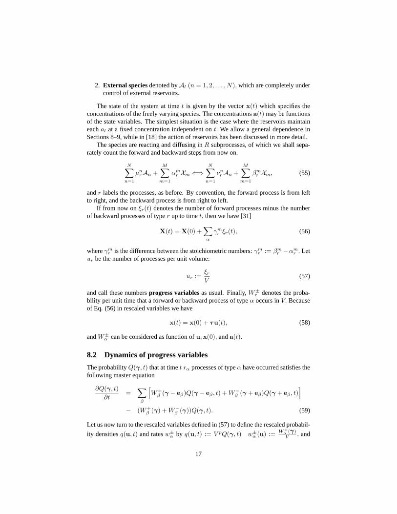
2. External speciesdenoted byAl (n = 1, 2, . . . , N), which are completely undercontrol of external reservoirs.

The state of the system at timet is given by the vectorx(t) which specifies theconcentrations of the freely varying species. The concentrationsa(t) may be functionsof the state variables. The simplest situation is the case where the reservoirs maintaineachal at a fixed concentration independent ont. We allow a general dependence inSections 8–9, while in [18] the action of reservoirs has been discussed in more detail.

The species are reacting and diffusing inR subprocesses, of which we shall sepa-rately count the forward and backward steps from now on.

N∑n=1

µnrAn +

M∑m=1

αmr Xm ⇐⇒

N∑n=1

νnr An +

M∑m=1

βmr Xm, (55)

andr labels the processes, as before. By convention, the forward process is from leftto right, and the backward process is from right to left.

If from now onξr(t) denotes the number of forward processes minus the numberof backward processes of typer up to timet, then we have [31]

X(t) = X(0) +∑α

γmr ξr(t), (56)

whereγmr is the difference between the stoichiometric numbers:γm

r := βmr −αm

r . Letur be the number of processes per unit volume:

ur :=ξr

V(57)

and call these numbersprogress variablesas usual. Finally,W±r denotes the proba-

bility per unit time that a forward or backward process of typeα occurs inV. Becauseof Eq. (56) in rescaled variables we have

x(t) = x(0) + τu(t), (58)

andW±α can be considered as function ofu,x(0), anda(t).

8.2 Dynamics of progress variables

The probabilityQ(γ, t) that at timet rα processes of typeα have occurred satisfies thefollowing master equation

∂Q(γ, t)∂t

=∑

β

[W+

β (γ − eβ)Q(γ − eβ , t) + W−β (γ + eβ)Q(γ + eβ , t)

]

− (W+β (γ) + W−

β (γ))Q(γ, t). (59)

Let us now turn to the rescaled variables defined in (57) to define the rescaled probabil-

ity densitiesq(u, t) and ratesw±α by q(u, t) := V pQ(γ, t) w±α (u) := W±α (γ)V , and

17

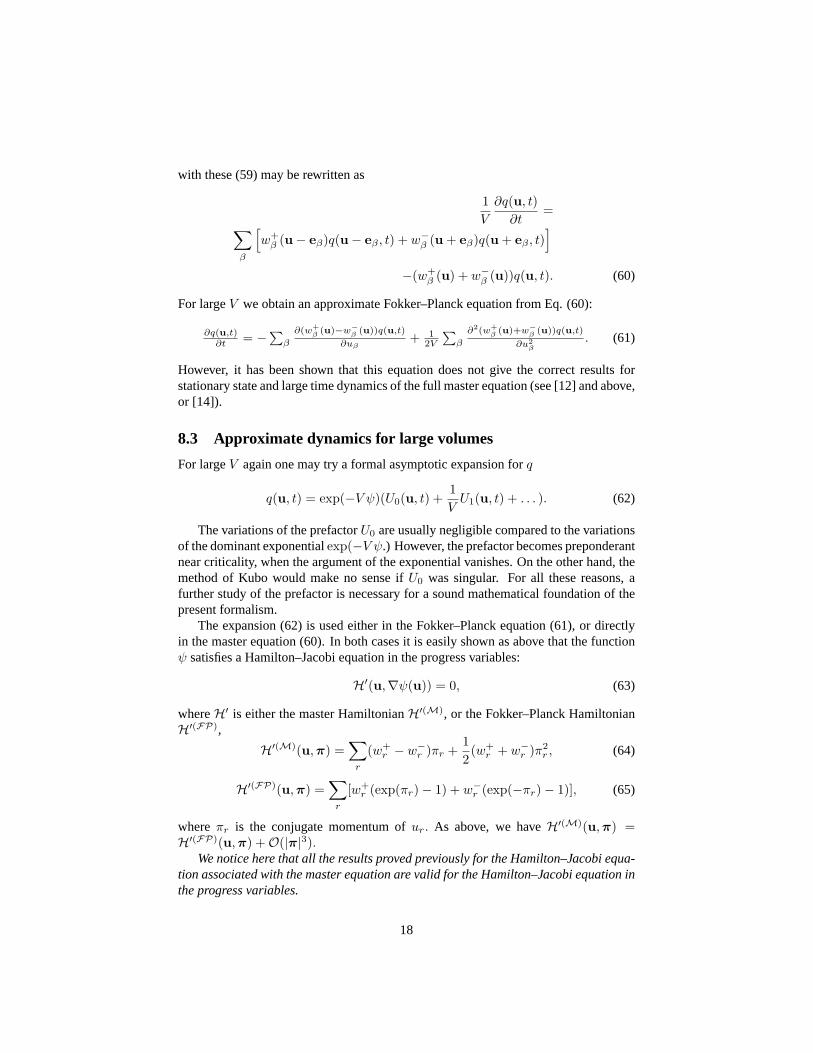
with these (59) may be rewritten as

1V

∂q(u, t)∂t

=∑

β

[w+

β (u− eβ)q(u− eβ , t) + w−β (u + eβ)q(u + eβ , t)]

−(w+β (u) + w−β (u))q(u, t). (60)

For largeV we obtain an approximate Fokker–Planck equation from Eq. (60):

∂q(u,t)∂t = −∑

β

∂(w+β (u)−w−β (u))q(u,t)

∂uβ+ 1

2V

∑β

∂2(w+β (u)+w−β (u))q(u,t)

∂u2β

. (61)

However, it has been shown that this equation does not give the correct results forstationary state and large time dynamics of the full master equation (see [12] and above,or [14]).

8.3 Approximate dynamics for large volumes

For largeV again one may try a formal asymptotic expansion forq

q(u, t) = exp(−V ψ)(U0(u, t) +1V

U1(u, t) + . . . ). (62)

The variations of the prefactorU0 are usually negligible compared to the variationsof the dominant exponentialexp(−V ψ.) However, the prefactor becomes preponderantnear criticality, when the argument of the exponential vanishes. On the other hand, themethod of Kubo would make no sense ifU0 was singular. For all these reasons, afurther study of the prefactor is necessary for a sound mathematical foundation of thepresent formalism.

The expansion (62) is used either in the Fokker–Planck equation (61), or directlyin the master equation (60). In both cases it is easily shown as above that the functionψ satisfies a Hamilton–Jacobi equation in the progress variables:

H′(u,∇ψ(u)) = 0, (63)

whereH′ is either the master HamiltonianH′(M), or the Fokker–Planck HamiltonianH′(FP),

H′(M)(u, π) =∑

r

(w+r − w−r )πr +

12(w+

r + w−r )π2r , (64)

H′(FP)(u, π) =∑

r

[w+r (exp(πr)− 1) + w−r (exp(−πr)− 1)], (65)

whereπr is the conjugate momentum ofur. As above, we haveH′(M)(u,π) =H′(FP)(u,π) +O(|π|3).

We notice here that all the results proved previously for the Hamilton–Jacobi equa-tion associated with the master equation are valid for the Hamilton–Jacobi equation inthe progress variables.

18

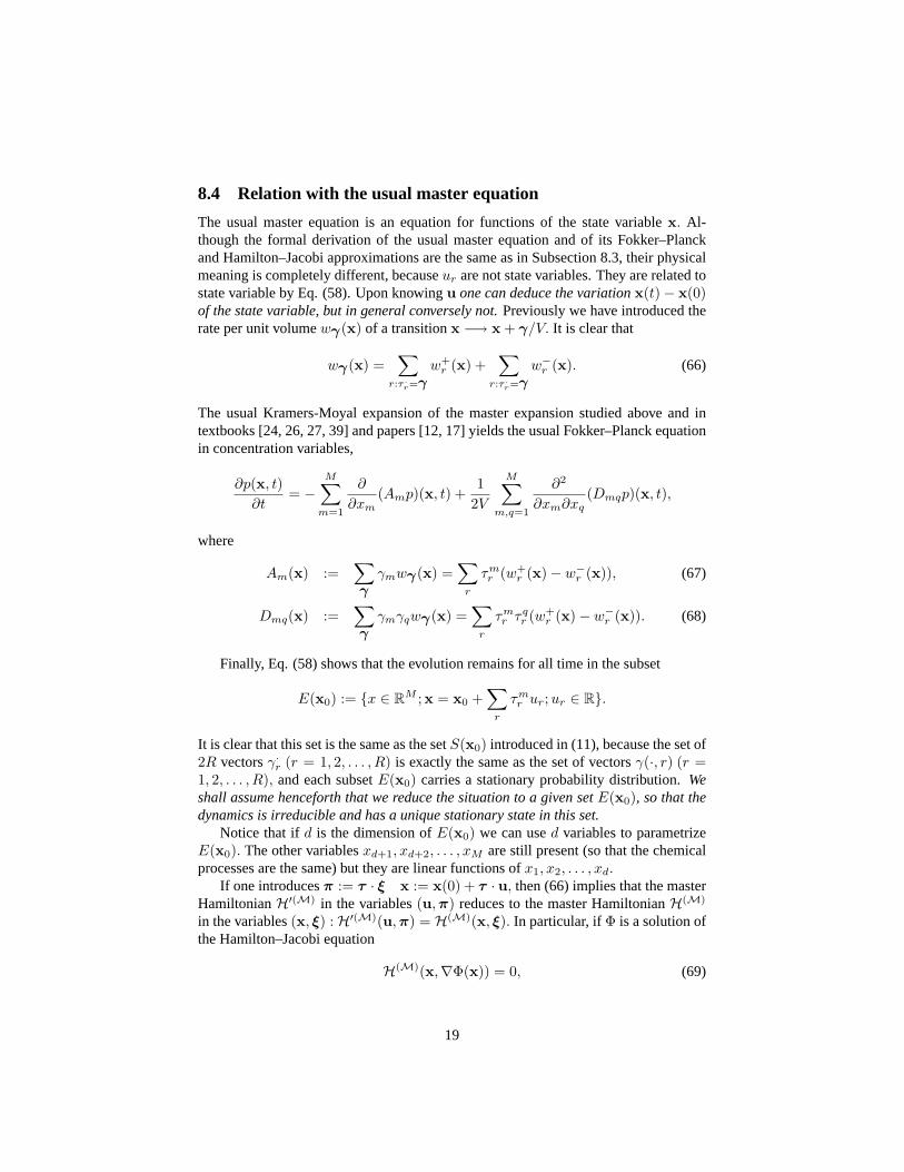
8.4 Relation with the usual master equation

The usual master equation is an equation for functions of the state variablex. Al-though the formal derivation of the usual master equation and of its Fokker–Planckand Hamilton–Jacobi approximations are the same as in Subsection 8.3, their physicalmeaning is completely different, becauseur are not state variables. They are related tostate variable by Eq. (58). Upon knowingu one can deduce the variationx(t)− x(0)of the state variable, but in general conversely not.Previously we have introduced therate per unit volumewγ(x) of a transitionx −→ x + γ/V. It is clear that

wγ(x) =∑

r:τ ·r=γw+

r (x) +∑

r:τ ·r=γw−r (x). (66)

The usual Kramers-Moyal expansion of the master expansion studied above and intextbooks [24, 26, 27, 39] and papers [12, 17] yields the usual Fokker–Planck equationin concentration variables,

∂p(x, t)∂t

= −M∑

m=1

∂

∂xm(Amp)(x, t) +

12V

M∑m,q=1

∂2

∂xm∂xq(Dmqp)(x, t),

where

Am(x) :=∑γ

γmwγ(x) =∑

r

τmr (w+

r (x)− w−r (x)), (67)

Dmq(x) :=∑γ

γmγqwγ(x) =∑

r

τmr τ q

r (w+r (x)− w−r (x)). (68)

Finally, Eq. (58) shows that the evolution remains for all time in the subset

E(x0) := x ∈ RM ;x = x0 +∑

r

τmr ur; ur ∈ R.

It is clear that this set is the same as the setS(x0) introduced in (11), because the set of2R vectorsγ·r (r = 1, 2, . . . , R) is exactly the same as the set of vectorsγ(·, r) (r =1, 2, . . . , R), and each subsetE(x0) carries a stationary probability distribution.Weshall assume henceforth that we reduce the situation to a given setE(x0), so that thedynamics is irreducible and has a unique stationary state in this set.

Notice that ifd is the dimension ofE(x0) we can used variables to parametrizeE(x0). The other variablesxd+1, xd+2, . . . , xM are still present (so that the chemicalprocesses are the same) but they are linear functions ofx1, x2, . . . , xd.

If one introducesπ := τ · ξ x := x(0) + τ · u, then (66) implies that the masterHamiltonianH′(M) in the variables(u, π) reduces to the master HamiltonianH(M)

in the variables(x, ξ) :H′(M)(u, π) = H(M)(x, ξ). In particular, ifΦ is a solution ofthe Hamilton–Jacobi equation

H(M)(x,∇Φ(x)) = 0, (69)

19

then the functionψ(u) := Φ(x(0) + τ · u) induces a solution of the Hamilton–Jacobiequation in the progress variable form:

H′(M)(u,∇ψ(u)) = 0, (70)

because∇ψ(u) = ∇Φ(x) · τ .But conversely, a solutionψ of the Hamilton–Jacobi equation (70) does not nec-

essarily produce a function in the state variablesx and a fortiori does not define asolution of Eq. (69).

8.5 Free energy and rate constantsin the unconstrained system

We consider now the vessel of volumeV, in which the2R processes take place, butnow we switch off the exchange of external speciesAn with the reservoirs (still main-taining the temperatureT constant), so thatthe concentrationsxm andan vary freelyaccording to the natural chemical processes(r = 1, 2, . . . , R) in the vessel. The statethen will reach a thermal equilibrium. At thermal equilibrium, the probability distribu-tion on the state space which consists now of the freely varying concentrationsxm andan is for largeV : peq(x,a) ∼ U0 exp(−V F (x,a)

kBT ), whereF is the free energy (of thestate(x,a)) per unit volume,kB is the Boltzmann constant,T is temperature, andU0

is a prefactor. At equilibrium, all processesr are supposed to satisfy detailed balance,as it is usual when dealing with realistic physical systems, written asymptotically forlargeV asw+

r (x,a) exp(− VkBT F (x,a)) = w−r (x,a) exp(− V

kBT F (x+ τ ·rV ,a+ t·r

V )),wheret := ν − µ. Therefore,

kBT log(w−rw+

r) =

∂F

∂x· τ +

∂F

∂a· t. (71)

For perfect gases or solutions one usually assumes that the rates are of themass actionform : w+

r (x) = k+r xα·

r w−r (x) = k−r xβ·r , wherek±r are temperature dependentrate coefficients. One can immediately check that the usual partial equilibrium form[13] of the free energy

F (x,a) =∑m

Fm(xm) +∑

n

Fn(an) (72)

(whereFm is the free energy of the ideal gas law at temperatureT and concentrationsx) does satisfy Eq. (71). In fact, the chemical potentials are

µm =∂F

∂xm=

dFm

dxm= kBT log(xm) + fm(T ), (73)

and Eq. (71) reduces to

kBT log(k+

r

k−r) =

∑m

τmr fm(T ) +

∑n

tnr fn(T ). (74)

20

Here eachfm is calculated using the partition functions of the internal degrees of free-dom of the speciesXm and Eq. (74) is the usual expression for the equilibrium constantKr,eq of the processr in term of the partition function of the internal degrees of free-dom of the species appearing in the given process.

In many circumstances, like for imperfect gases or solutions, electrolytes, etc. oneneeds a more general formulation of the free energyF, not necessarily of the form (72).This is why we shall work with the most general form of the free energy.

From Eq. (71) it follows for allr

w+r (x,a) exp

(1

kBT∂F (x,a))

∂ur− 1

)+ w−r (x,a) exp

(− 1

kBT∂F (x,a))

∂ur− 1

)= 0, (75)

where ∂F∂ur

=∑

m∂F

∂xmτmr + ∂F

∂untnr , so that 1

kBT F satisfies the Hamilton–Jacobi equa-

tion (63):H′(M)(u, 1kBT

∂F∂u ) = 0 withH′(M) given by (65), where inw±r the variables

arex = x(0) + τ · u a = a(0) + t · u.

9 Dissipation

9.1 Dissipation of information

From now on, we shall assume again that on a given setE(x0) the state of the vesselreaches a stationary statep(x) ∼ U0 exp(−V Φ(x)) with the concentrationsa beingentirely controlled by the reservoirs and having fixed variationsa(t).

The statex(t) macroscopically evolves according to the deterministic equationsdxdt = A(x) = τ · (w+(x(t))−w−(x(t))). The value of the state functionΦ evolvesas

dΦdt

= ∇Φ(x(t))x(t) =∑m,r

(w+r (x(t))− w+

r (x(t)))∂Φ∂ur

. (76)

We know from Subsection (8.5) thatH′(M)(u,∇Φ(u)) = 0. But ex − 1 ≥ x, so

that0 =∑

r

[w+

r (exp( ∂Φ∂ur

)− 1) + w−r (exp(− ∂Φ∂ur

)− 1)]≥ ∑

r(w+r −w+

r ) ∂Φ∂ur

. As

a consequence, we obtain the inequalitydΦdt ≤ 0, where equality is attained if and

only if w+r ∂Φ/∂ur = w−r ∂Φ/∂ur for eachr. In particular, if the deterministic state

reaches a stationary pointx(0), for which A(x(0)) = 0, thendΦ/dt = 0, and either∂Φ/∂ur = 0, or w+

r = w−r = 0.The quantitydΦ/dt computed along a deterministic trajectory is always negative.

It can be interpreted as a dissipation of information per unit time.In fact, V Φ(x) can be considered as the average information which is obtained

when the system is observed in the statex rather then being stochastically distributedwith the stationary probability distributionps(x) ∼ exp(−V Φ(x)), which is the stateof lowest information, when the system is coupled to the various reservoirs of heat andof chemical speciesAn. Along a deterministic pathΦ decreases with time while thestatex tends to a deterministic stationary state which is a local minimum ofΦ.

21

9.2 Dissipation of energy

The variation of free energy along the deterministic trajectory is

dF

dt=

∑

i

∂F

∂xi

dxi

dt+

∑

i

∂F

∂al

dal

dt, (77)

or,

dF

dt=

∑

i

∂F

∂xi

dxi

dt+

∑

i

∂F

∂al

[dal

dt

]

c

−∑

i

∂F

∂al

([dal

dt

]

c

− dal

dt

), (78)

where[dal

dt

]c

is the variation ofal due to the chemical processes. It turns out [18][p.

684] thatdFdt −w ≤ 0, wherew := −∑

l ml

([dal

dt

]c− dal

dt

), andthe quantitydF

dt −wis the dissipation of energy in the system per unit time.

9.3 Inequality between the dissipation of informationand that of energy

It is proved in Appendix A of [18] that the dissipation of information and the dissipationof energy satisfy the fundamental inequality1kBT

(dFdt − w

) ≤ dΦdt ≤ 0, so that in

absolute value the dissipation of information is always less than the dissipation ofenergy. Moreover, there is equality if and only if we have an equilibrium situation.

10 Acknowledgements

The present work has partly been supported by the National Science Foundation Hun-gary (Nos T037491 and T047132).

References

[1] Arnold, L.: On the consistency of the mathematical models of chemical reactions,In: Dynamics of synergetic systems, Ed. H. Haken, Springer, Berlin, 1980, pp.107-118.

[2] Courant, R. and Hilbert, D.:Methods of mathematical physics, Interscience, NewYork, 1953.

[3] Cover, T. M. and Thomas, J. A.:Elements of information theory, Wiley, NewYork, 1991.

[4] Englman, R. and Yahalom, A.: Variational procedure for time dependent pro-cesses,Physical Review E, 69 (2004), 026120(10 pages).

[5] Erdi, P., Toth, J.: Mathematical models of chemical reactions. Theory and ap-plications of deterministic and stochastic models, Princeton University Press,Princeton, 1989.

22

[6] Erdi, P., Toth, J.: Stochastic reaction kinetics—Nonequilibrium thermodynamicsof the state space?Reaction Kinetics and Catalysis Letters4 (1976), 81–85.

[7] Feynman, R. P. and Hibbs, A.:Quantum mechanics and path integrals, McGraw-Hill, New York, 1965.

[8] Forster, D.:Hydrodynamic fluctuations, broken symmetry, and correlation func-tions, Frontiers in physics, Vol. 47, Benjamin Cummings, Reading, MA, 1975.

[9] Gardiner, H.:Handbook of stochastic methods, Springer, Berlin, 1983.

[10] Gaveau, B., Martinas, K., Moreau, M., Toth, J.: Entropy, extropy and informationpotential in stochastic systems far from equilibrium,Physica A305(2002), 445–466.

[11] Gaveau, B.; Moreau, M. and Toth, J.: Decay of the metastable state: differ-ent predictions between discrete and continuous models,Letters in MathematicalPhysics37 (1996), 285–292.

[12] Gaveau, B.; Moreau, M. and Toth, J.: Master equation and Fokker–Planck equa-tion: Comparison of entropy and rate constants,Letters in Mathematical Physics40 (1997), 101–115.

[13] Gaveau, B.; Moreau, M. and Toth, J.: Dissipation of energy and information innonequilibrium reaction-diffusion systems,Physical Review E58 (11) (1998),5351–5354.

[14] Gaveau, B.; Moreau, M. and Toth, J.: Variational nonequilibrium thermodynam-ics of reaction-diffusion systems. I. The information potential,Journal of Chemi-cal Physics111(17) (1999), 7736–7747.

[15] Gaveau, B.; Moreau, M. and Toth, J.: Variational nonequilibrium thermodynam-ics of reaction-diffusion systems. II. Path integrals, large fluctuations and rateconstants,Journal of Chemical Physics111(17) (1999), 7748–7757.

[16] Gaveau, B.; Moreau, M. and Toth, J.:Path-integrals from peV to TeV, (Florence,August 1998), Casalbroni R., ed., World Scientific, Singapore, 1999, pp. 52.

[17] Gaveau, B.; Moreau, M. and Toth, J.: Information potential and transition tocriticality for certain two-species chemical systems,Physica A277(2000), 455–468.

[18] Gaveau, B.; Moreau, M. and Toth, J.: Variational nonequilibrium thermodynam-ics of reaction-diffusion systems. III. Progress variables and dissipation of energyand information,Journal of Chemical Physics115(2) (2001), 680–690.

[19] Gaveau, B. and Schulman, L. S.: Master equation based formulation of nonequi-librium statistical mechanics,Journal of Mathematical Physics37 (8) (1996),3897–3932.

23

[20] Gaveau, B. and Schulman, L. S.: A general framework for non-equilibrium phe-nomena: The master equation and its formal consequences,Phys. Lett. A229(6)(1997), 347–353.

[21] Gaveau, B. and Schulman, L. S.: Theory of nonequilibrium first-order phase tran-sitions for stochastic dynamics,Journal of Mathematical Physics39 (3) (1998),1517–1533.

[22] Gyarmati, I.: On the governing principle of dissipative processes and its extensionto nonlinear problems,Annalen der Physik, 23 (1969), 353–378.

[23] Gyarmati, I.: Non-equilibrium thermodynamics. Field theory and variationalprinciples, Springer Verlag, 1970.

[24] De Groot, S. R. and Mazur, P.:Nonequilibrium thermodynamics, Dover, NewYork, 1984.

[25] Horn, F. J. M. and Jackson, R.: General mass action kinetics,Archive for RationalMechanics and Analysis47 (1972), 81–116.

[26] Keizer, J.: Statistical thermodynamics of nonequilibrium processes, Springer,New York, 1987.

[27] Kubo, R.:Statistical mechanics, North Holland, Amsterdam, 1988.

[28] Kubo, R.; Matsuo, K. and Kitahara, K.: Fluctuation and relaxation of macrovari-ables,Journal of Statistical Physics, 9 (1973), 51–96.

[29] Kubo, R.; Toda, M. and Hashitsume, N. In:Statistical physics II, Springer, NewYork, 1986.

[30] Kullback, S.:Information theory and statistics, Wiley, New York, 1959.

[31] Kurtz, T. G.: The relationship between stochastic and deterministic models inchemical reactions,Journal of Chemical Physics57 (1973), 2976–2978.

[32] Landau, L. D. and Lifsic, E. M.:Mechanics: Volume 1, Butterworth-Heinemann;3rd edition, 1976.

[33] Landau, L. and Lifsic, E. M.:Statistical physics, Pergamon, Oxford, 1980.

[34] Lemarchand, H.: Asymptotic solution of the master equation near a nonequilib-rium transition,Physica A101(1980), 518–534.

[35] Lemarchand, H. and Nicolis, G.: Stochastic analysis of symmetry-breaking bi-furcations: master equation approach,Journal of Statistical Physics, 37 (1984),609–629.

[36] Ludwig, D.: Persistence of dynamical systems under random perturbations,SIAMRev.17 (1975), 605–640.

[37] Moreau, M.:Letters in Mathematical Physics1 (1975), 7.

24

[38] Moreau, M.: Note on the entropy production in a discrete Markov system,Journalof Mathematical Physics19 (12) (1978), 2494–2498.

[39] Nicolis, G. and Prigogine, I.:Self-organization in nonequilibrium systems, Wiley,New York, 1977.

[40] Prigogine, I.:Nonequilibrium statistical mechanics, Wiley, New York, 1962.

[41] Prigogine, I. and Nicolis, G.: In:From theoretical physics to biology, Ed. M.Marois, Karger, Basel, 1973.

[42] Ruelle, D.:Statistical mechanics, Benjamin, New York, 1970.

[43] Schulman, L. S.: In:Finite size scaling and numerical simulation of statisticalsystems, Privman, V. ed., World Scientific, Singapore, 1990.

[44] Sieniutycz, S.: Some thermodynamic aspects of development and bistability incomplex multistage systems,Open Sys. & Information Dyn.7 (2000), 309–326.

[45] Sieniutycz, S.: Optimality of nonequilibrium systems and problems of statisticalthermodynamics,International Journal of Heat and Mass Transfer, 45 (2002),1545–1561.

[46] Toth, J. andErdi, P.: Indispensability of stochastic models, In:Nonlinear dynam-ics and exotic kinetic phenomena in chemical systems,(Gy. Bazsa ed.) Debrecen,Budapest, Godollo, 1992, pp. 117–143 (in Hungarian).

[47] Van, P.: On the structure of the ’Governing Principle of Dissipative Processes’,Journal of Non-equilibrium Thermodynamics21 (1) (1996) 17–29.

[48] Van, P. and Muschik, W.: The structure of variational principles in non-equilibrium thermodynamics,Physical Review E52 (4) (1995), 3584–3590.

[49] Van, P. and Nyıri, B.: Hamilton formalism and variational principle construction,Annalen der Physik(Leipzig)8 (1999), 331–354.

[50] Ventsel, A. and Freidlin, M.: On small random perturbation of dynamical sys-tems,Russian Math. Surveys25 (1970), 1–55.

[51] Vlad, M. O. and Ross, J.: Fluctuation-dissipation relations for chemical systemsfar from equilibrium,Journal of Chemical Physics100(10) (1994), 7268–7278.

[52] Vlad, M. O. and Ross, J.: Random paths and fluctuation-dissipation dynamics forone-variable chemical systems far from equilibrium,Journal of Chemical Physics100(10) (1994), 7279–7294.

[53] Vlad, M. O. and Ross, J.: Thermodynamic approach to nonequilibrium chemicalfluctuations,Journal of Chemical Physics100(10) (1994), 7295–7309.

[54] Zheng, Q.; Ross, J.; Hunt, K. L. C. and Hunt, P. M.: Stationary solutions of themaster equation for single and mulitintermediate autocatalytic chemical systems,Journal of Chemical Physics96 (1) (1992), 630–641.

25