Variational Formulation & the Galerkin Method
50
Institute of Structural Engineering Page 1 Method of Finite Elements I Variational Formulation & the Galerkin Method Dr. Konstantinos Agathos Institute of Structural Engineering ETH Zürich 8 April 2020
Transcript of Variational Formulation & the Galerkin Method
Institute of Structural Engineering Page 1
Method of Finite Elements I
Variational Formulation & the Galerkin Method
Dr. Konstantinos Agathos
Institute of Structural Engineering ETH Zürich
8 April 2020
Institute of Structural Engineering Page 2
Method of Finite Elements I
Today’s Lecture Contents:
• Introduction
• Strong form
– Strong form of a 1D bar
– Strong form solution for a 1D bar
• Weak form
– Potential minimization
– Principle of Virtual Work
– Galerkin Method
– Weak form solution
Institute of Structural Engineering Page 3
Method of Finite Elements I
Learning goals:
• Understanding strong and weak forms through a simple example
• Demonstrating the equivalence between the two as well as the differences
• Demonstrating the equivalence between alternative weak formulations
• Understanding the advantages of weak formulations in the development of approximate solution methods
Institute of Structural Engineering Page 4
Method of Finite Elements I
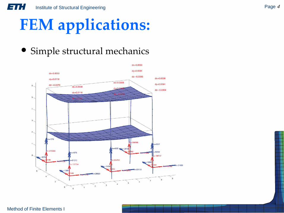
FEM applications:
• Simple structural mechanics
Institute of Structural Engineering Page 5
Method of Finite Elements I
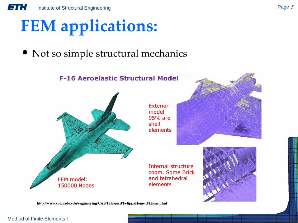
FEM applications:
• Not so simple structural mechanics
Institute of Structural Engineering Page 6
Method of Finite Elements I
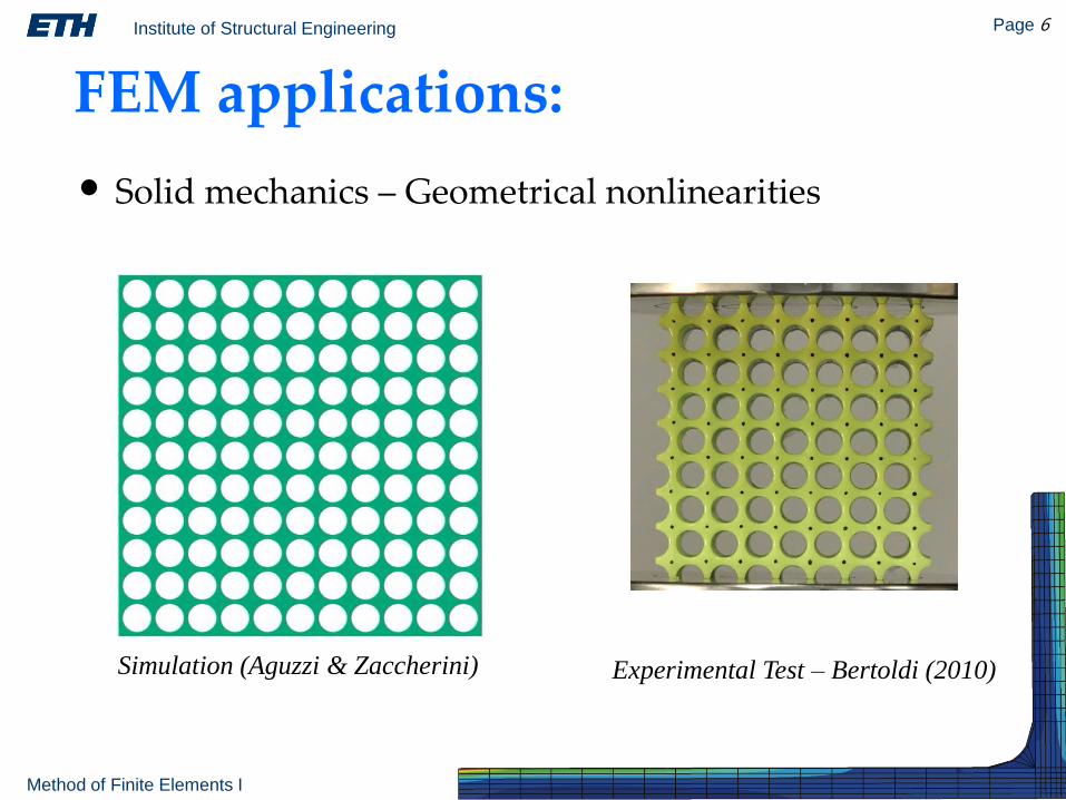
FEM applications:
• Solid mechanics – Geometrical nonlinearities
Experimental Test – Bertoldi (2010) Simulation (Aguzzi & Zaccherini)
Institute of Structural Engineering Page 7
Method of Finite Elements I
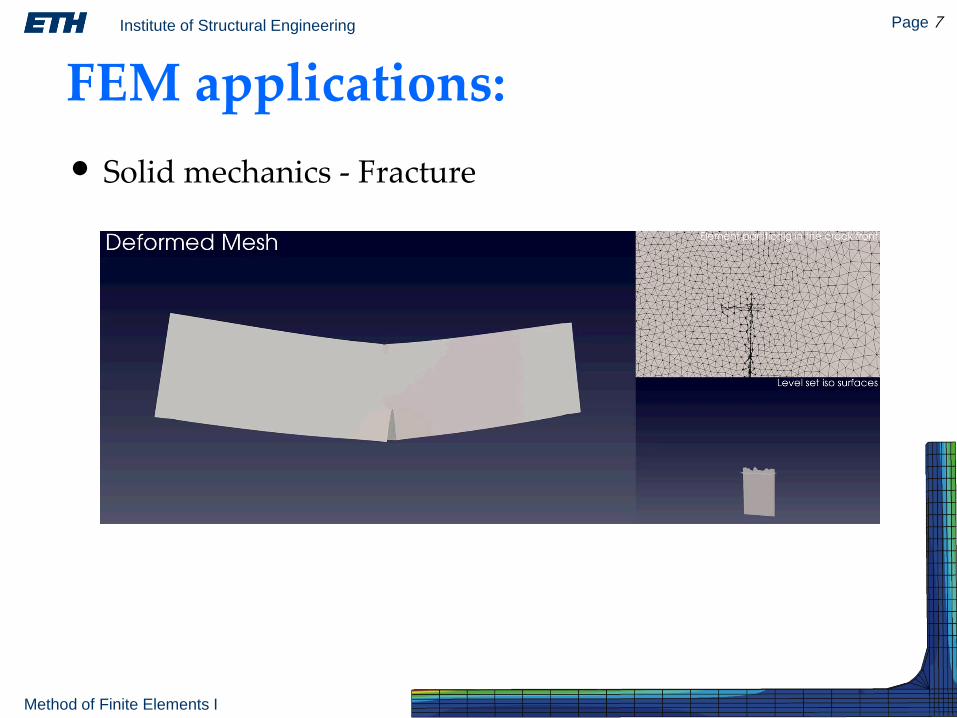
FEM applications:
• Solid mechanics - Fracture
Institute of Structural Engineering Page 8
Method of Finite Elements I
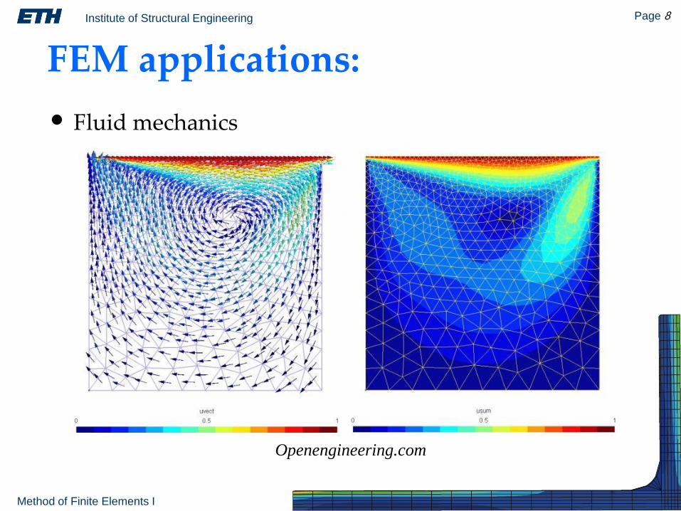
FEM applications:
• Fluid mechanics
Openengineering.com
Institute of Structural Engineering Page 9
Method of Finite Elements I
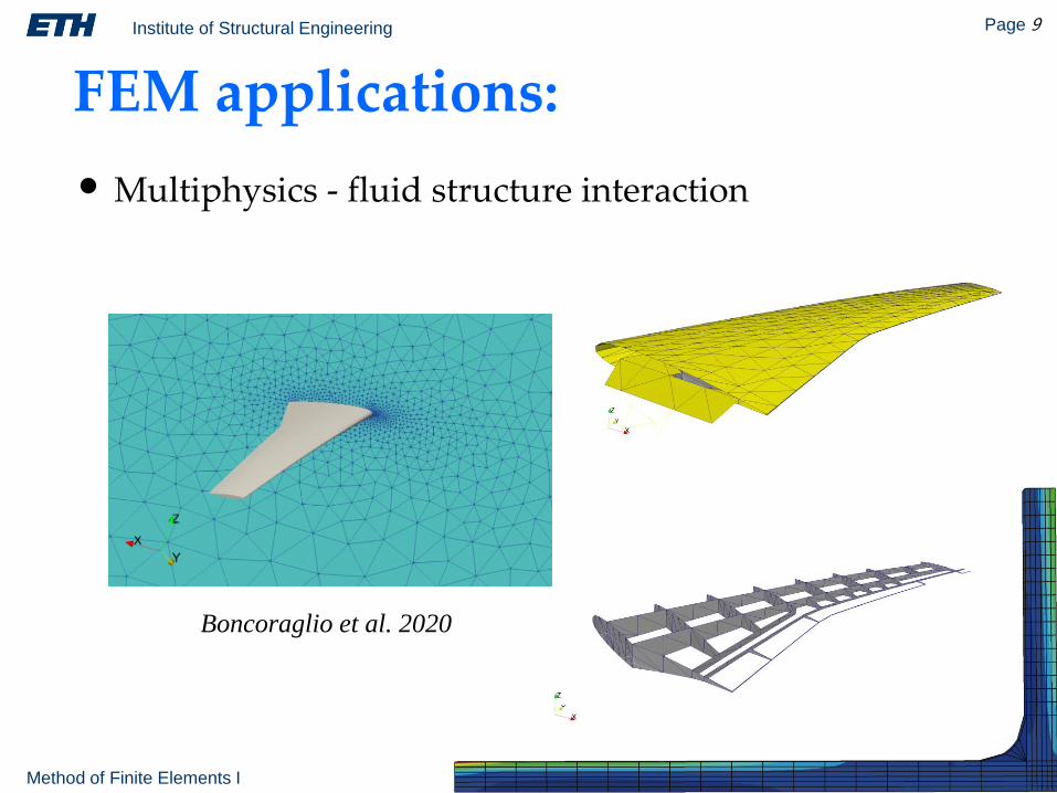
FEM applications:
• Multiphysics - fluid structure interaction
Boncoraglio et al. 2020
Institute of Structural Engineering Page 10
Method of Finite Elements I
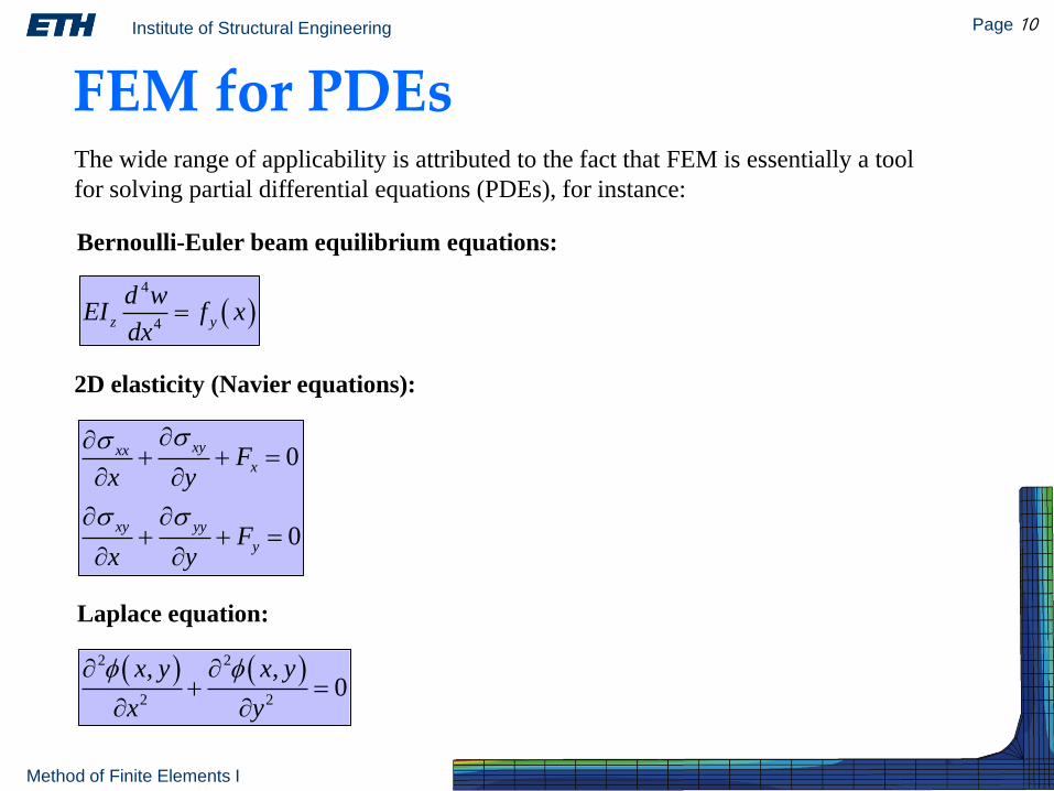
FEM for PDEsThe wide range of applicability is attributed to the fact that FEM is essentially a tool
for solving partial differential equations (PDEs), for instance:
Bernoulli-Euler beam equilibrium equations:
2D elasticity (Navier equations):
Laplace equation:
4
4z y
d wEI f x
dx
0
0
xyxxx
xy yy
y
Fx y
Fx y
2 2
2 2
, ,0
x y x y
x y
Institute of Structural Engineering Page 11
Method of Finite Elements I
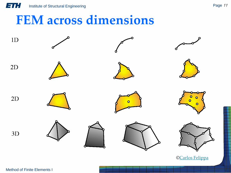
©Carlos Felippa
FEM across dimensions
Institute of Structural Engineering Page 12
Method of Finite Elements I
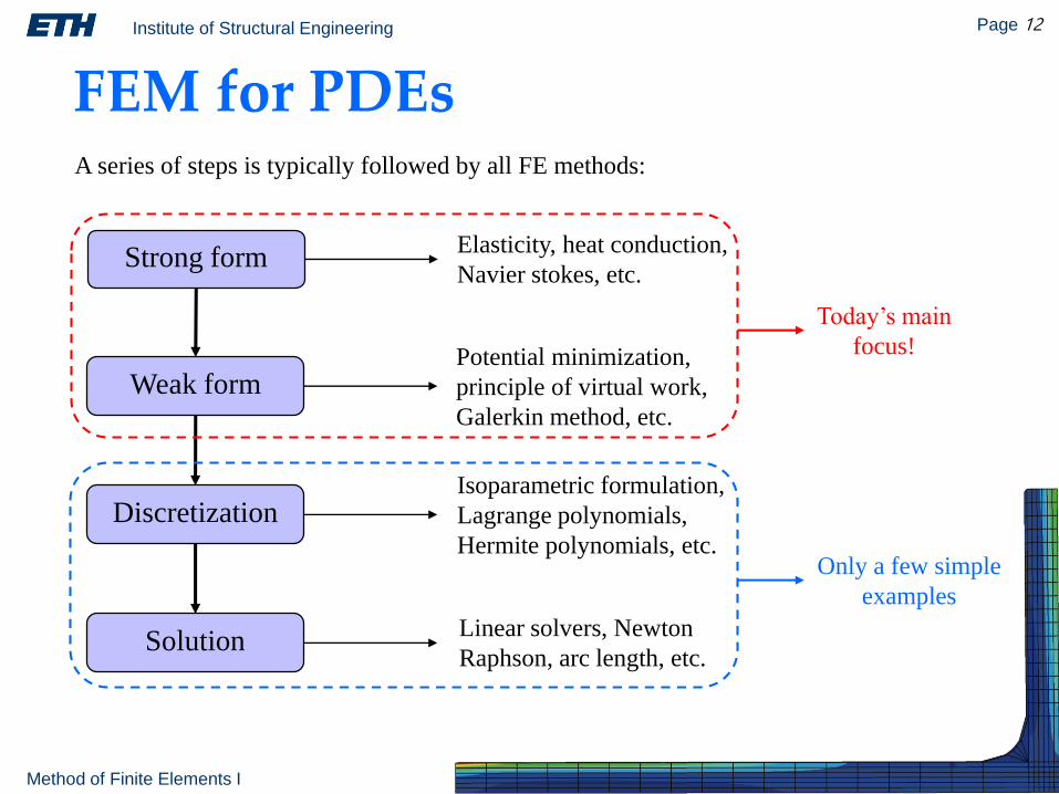
FEM for PDEsA series of steps is typically followed by all FE methods:
Strong form
Weak form
Discretization
Solution
Elasticity, heat conduction,
Navier stokes, etc.
Potential minimization,
principle of virtual work,
Galerkin method, etc.
Isoparametric formulation,
Lagrange polynomials,
Hermite polynomials, etc.
Linear solvers, Newton
Raphson, arc length, etc.
Today’s main
focus!
Only a few simple
examples
Institute of Structural Engineering Page 13
Method of Finite Elements I
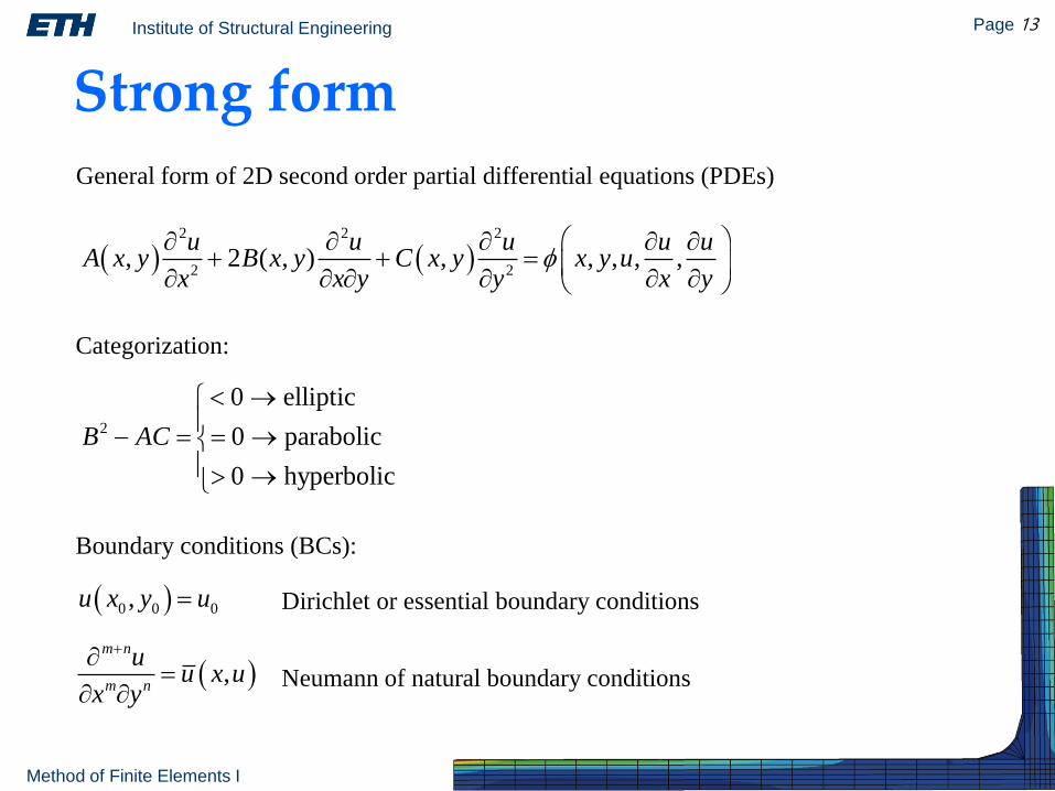
Strong formGeneral form of 2D second order partial differential equations (PDEs)
2 2 2
2 2, 2 ( , ) , , , , ,
u u u u uA x y B x y C x y x y u
x x y y x y
Dirichlet or essential boundary conditions
2
0 elliptic
0 parabolic
0 hyperbolic
B AC
Categorization:
0 0 0,u x y u
,m n
m n
uu x u
x y
Boundary conditions (BCs):
Neumann of natural boundary conditions
Institute of Structural Engineering Page 14
Method of Finite Elements I
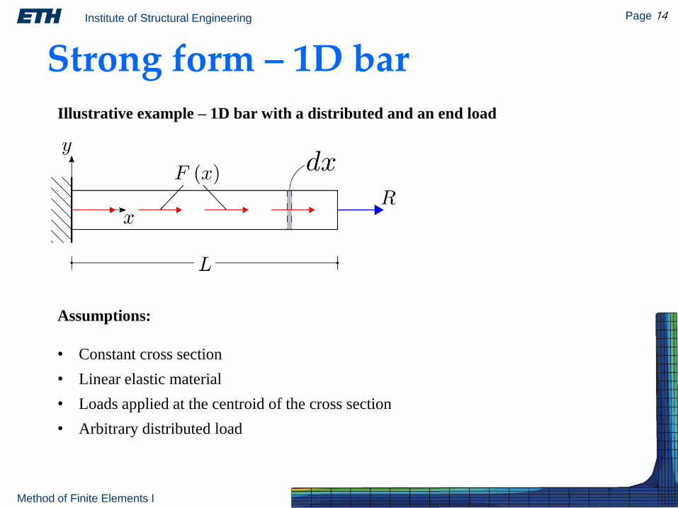
Strong form – 1D bar
Assumptions:
• Constant cross section
• Linear elastic material
• Loads applied at the centroid of the cross section
• Arbitrary distributed load
Illustrative example – 1D bar with a distributed and an end load
Institute of Structural Engineering Page 15
Method of Finite Elements I
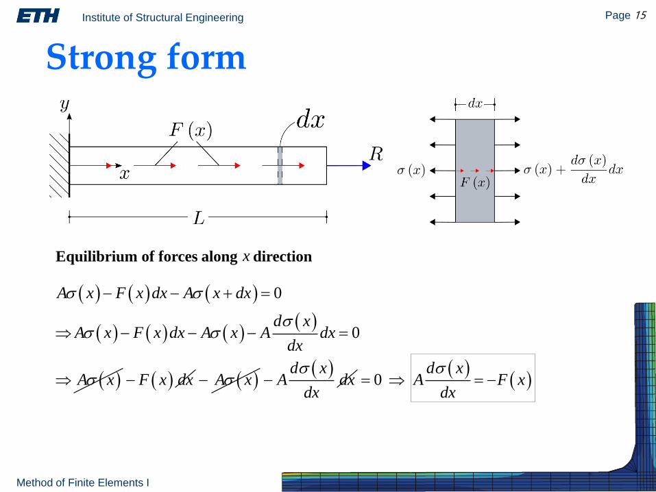
Equilibrium of forces along directionx
0
0
A x F x dx A x dx
d xA x F x dx A x A dx
dx
A x
F x dx A x d x
A dxdx
0
d xA F x
dx
Strong form
Institute of Structural Engineering Page 16
Method of Finite Elements I
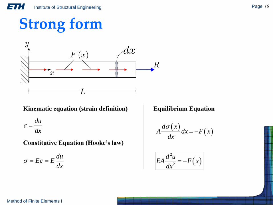
Constitutive Equation (Hooke’s law)
duE E
dx
Kinematic equation (strain definition)
du
dx
Equilibrium Equation
2
2
d xA dx F x
dx
d uEA F x
dx
Strong form
Institute of Structural Engineering Page 17
Method of Finite Elements I
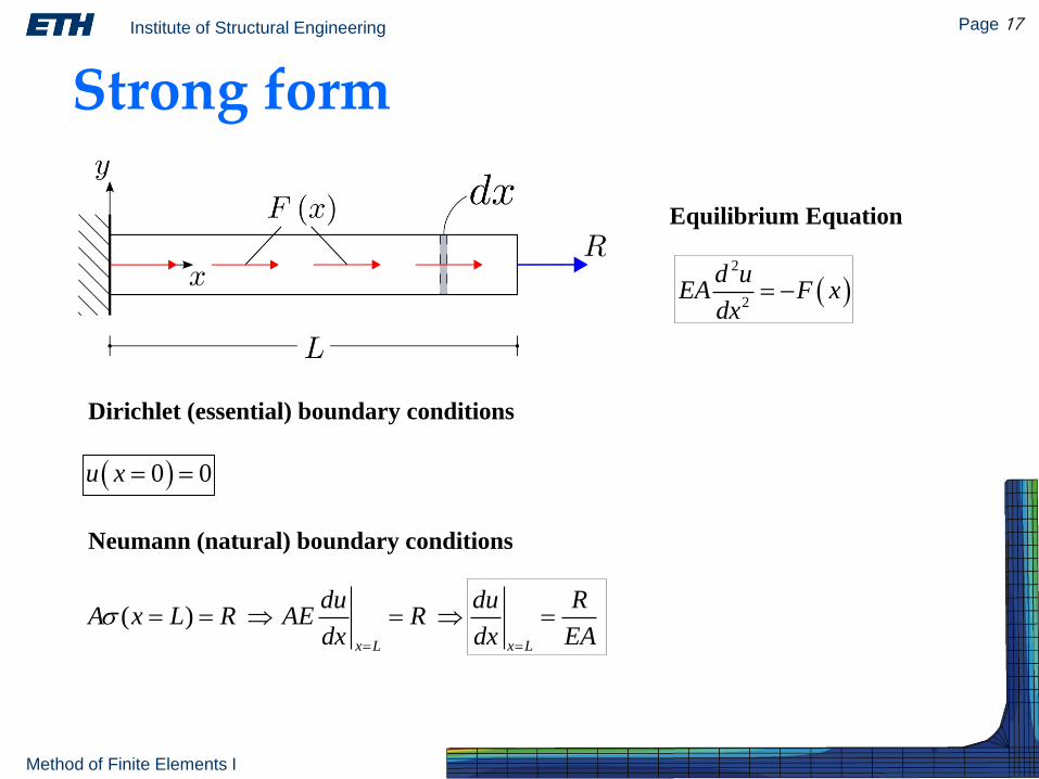
Neumann (natural) boundary conditions
( )x L x L
du du RA x L R AE R
dx dx EA
Dirichlet (essential) boundary conditions
0 0u x
Equilibrium Equation
2
2
d uEA F x
dx
Strong form

Institute of Structural Engineering Page 18
Method of Finite Elements I
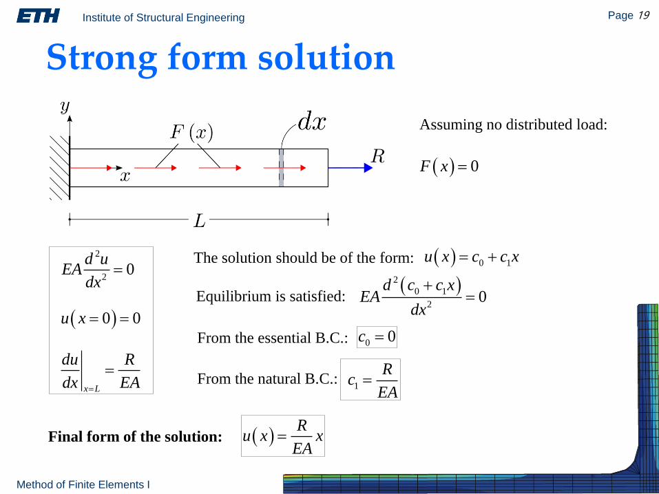
Strong form solution
Assuming no distributed load:
0F x
2
20
d uEA
dx
x L
du R
dx EA
0 0u x
Institute of Structural Engineering Page 19
Method of Finite Elements I
Strong form solution
Assuming no distributed load:
0F x
2
20
d uEA
dx
x L
du R
dx EA
0 0u x
The solution should be of the form: 0 1u x c c x
Equilibrium is satisfied: 2
0 1
20
d c c xEA
dx
From the essential B.C.: 0 0c
From the natural B.C.:1
Rc
EA
Final form of the solution: R
u x xEA
Institute of Structural Engineering Page 20
Method of Finite Elements I
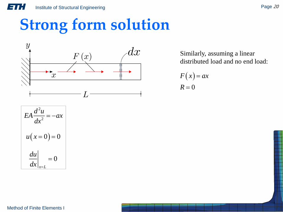
Strong form solution
Similarly, assuming a linear
distributed load and no end load:
0
F x ax
R
2
2
d uEA ax
dx
0x L
du
dx
0 0u x
Institute of Structural Engineering Page 21
Method of Finite Elements I
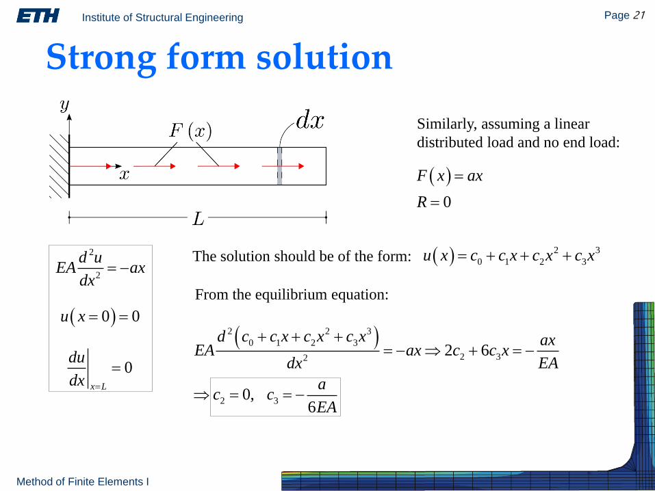
Strong form solution
Similarly, assuming a linear
distributed load and no end load:
0
F x ax
R
2
2
d uEA ax
dx
0x L
du
dx
0 0u x
The solution should be of the form: 2 3
0 1 2 3u x c c x c x c x
From the equilibrium equation:
2 2 3
0 1 2 3
2 32
2 3
2 6
0,6
d c c x c x c x axEA ax c c x
dx EA
ac c
EA
Institute of Structural Engineering Page 22
Method of Finite Elements I
2 3
0 1 2 3u x c c x c x c x
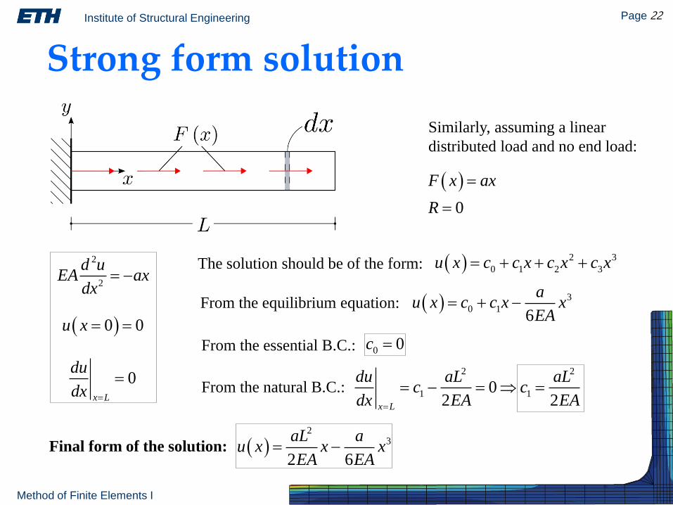
Strong form solution
Similarly, assuming a linear
distributed load and no end load:
0
F x ax
R
2
2
d uEA ax
dx
0x L
du
dx
0 0u x
The solution should be of the form:
From the equilibrium equation: 3
0 16
au x c c x x
EA
From the essential B.C.: 0 0c
From the natural B.C.:2 2
1 102 2x L
du aL aLc c
dx EA EA
Final form of the solution: 2
3
2 6
aL au x x x
EA EA
Institute of Structural Engineering Page 23
Method of Finite Elements I
Strong form solution
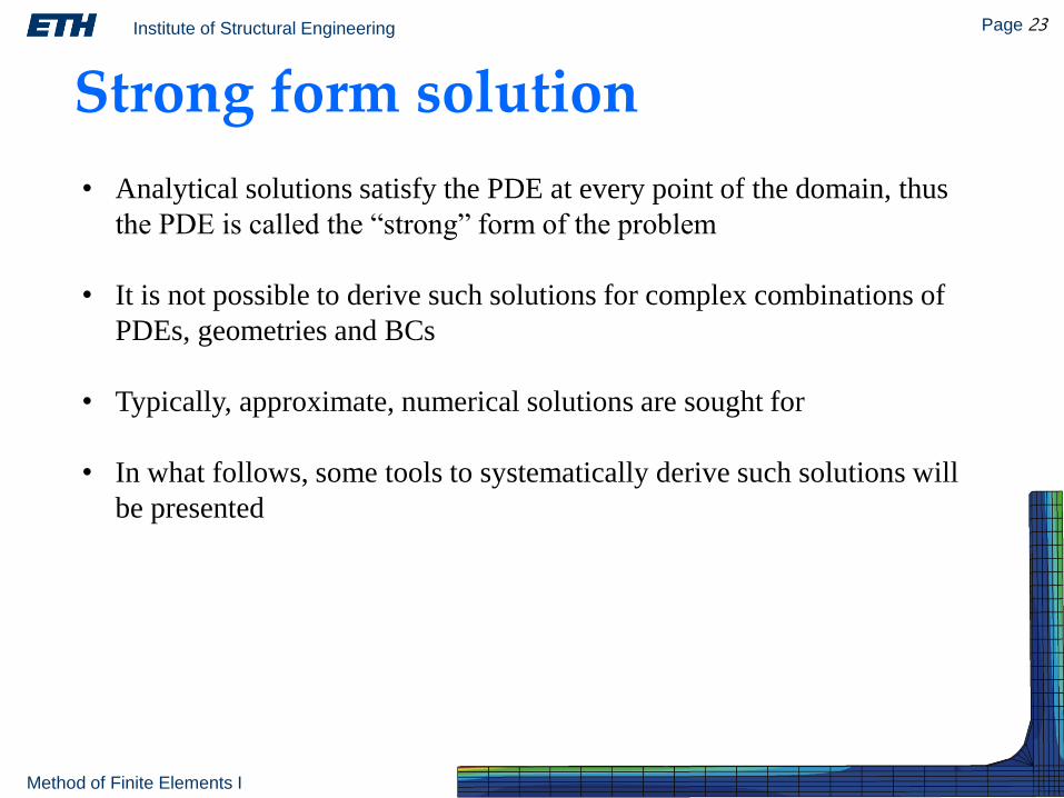
• Analytical solutions satisfy the PDE at every point of the domain, thus
the PDE is called the “strong” form of the problem
• It is not possible to derive such solutions for complex combinations of
PDEs, geometries and BCs
• Typically, approximate, numerical solutions are sought for
• In what follows, some tools to systematically derive such solutions will
be presented
Institute of Structural Engineering Page 24
Method of Finite Elements I
Potential minimization
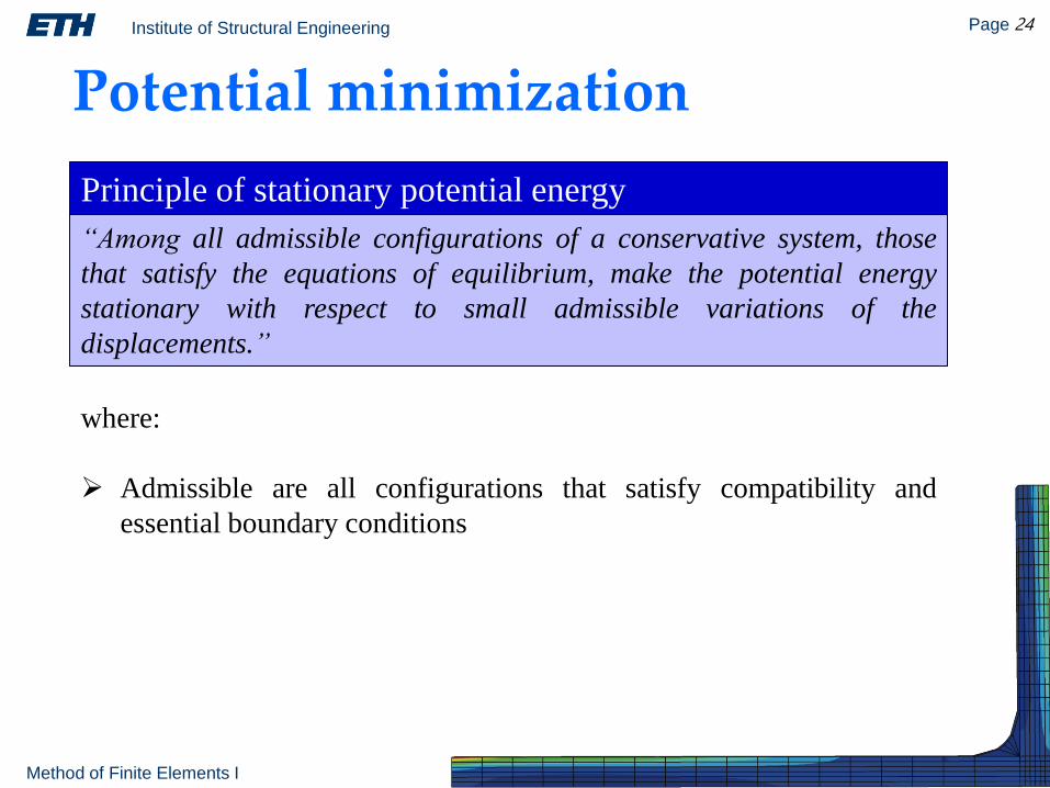
Principle of stationary potential energy
“Among all admissible configurations of a conservative system, those
that satisfy the equations of equilibrium, make the potential energy
stationary with respect to small admissible variations of the
displacements.”
where:
Admissible are all configurations that satisfy compatibility and
essential boundary conditions
Institute of Structural Engineering Page 25
Method of Finite Elements I
Potential minimization
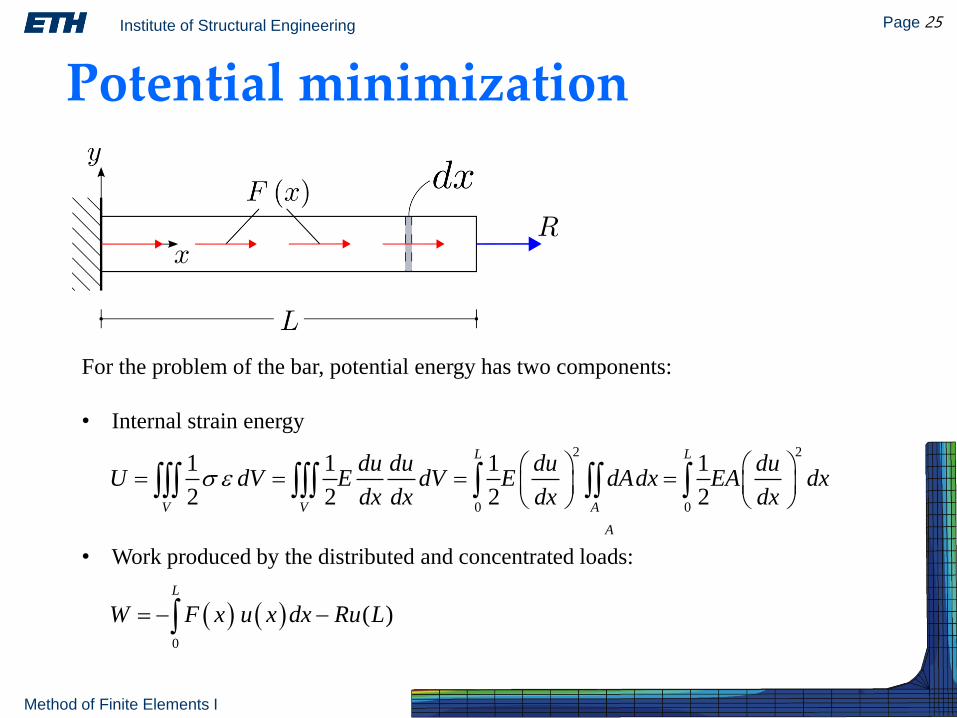
For the problem of the bar, potential energy has two components:
• Internal strain energy
• Work produced by the distributed and concentrated loads:
2 2
0 0
1 1 1 1
2 2 2 2
L L
V V A
A
du du du duU dV E dV E dAdx EA dx
dx dx dx dx
0
( )
L
W F x u x dx Ru L
Institute of Structural Engineering Page 26
Method of Finite Elements I
Potential minimization
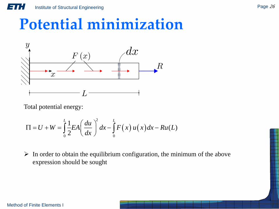
Total potential energy:
In order to obtain the equilibrium configuration, the minimum of the above
expression should be sought
2
0 0
1( )
2
L Ldu
U W EA dx F x u x dx Ru Ldx
Institute of Structural Engineering Page 27
Method of Finite Elements I
Potential minimization
The expression derived for the total potential energy is a functional, i.e. a mapping
from a function space to the real numbers.
In simpler words:
• Functions take numbers as input and return numbers as output, i.e. they map
numbers to numbers
• Functionals take functions as input and return numbers as output, i.e. they map
functions to numbers
To minimize a functional, we need some additional definitions
Institute of Structural Engineering Page 28
Method of Finite Elements I
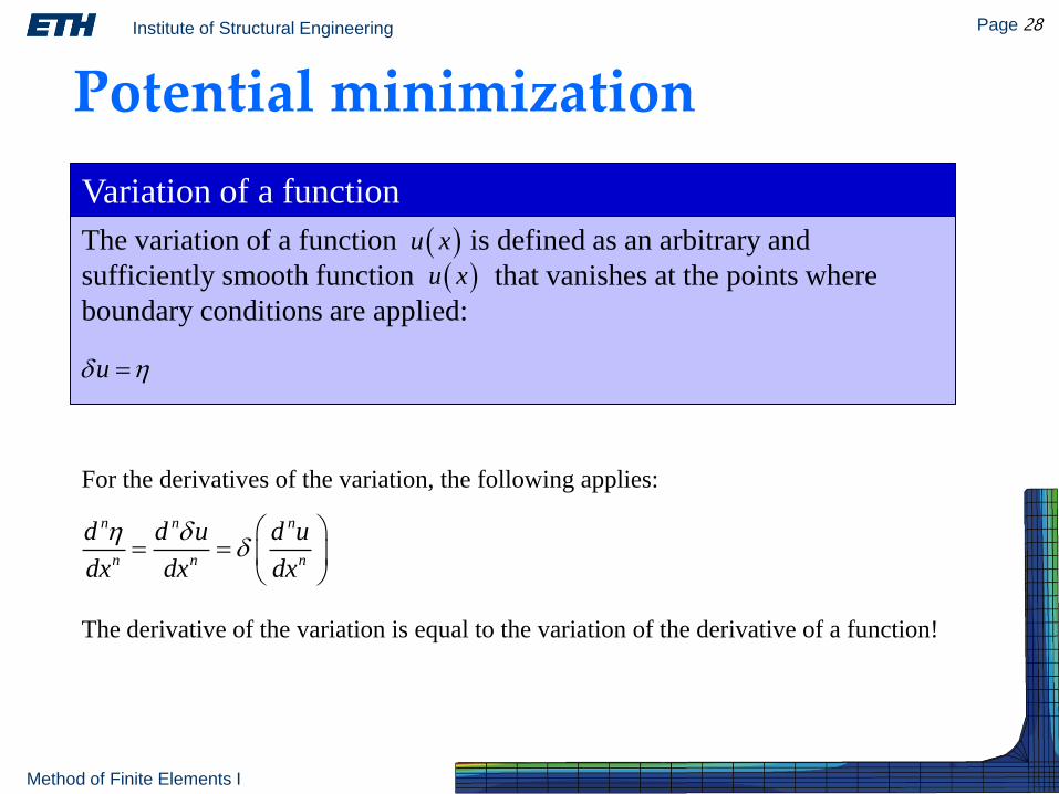
For the derivatives of the variation, the following applies:
The derivative of the variation is equal to the variation of the derivative of a function!
Potential minimization
Variation of a function
The variation of a function is defined as an arbitrary and
sufficiently smooth function that vanishes at the points where
boundary conditions are applied:
n n n
n n n
d d u d u
dx dx dx
u
u x
u x
Institute of Structural Engineering Page 29
Method of Finite Elements I
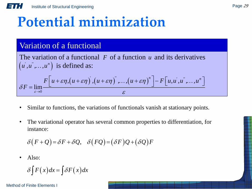
Potential minimization
Variation of a functional
The variation of a functional of a function and its derivatives
is defined as:
0
, , , , , , , ,lim
n nF u u u u F u u u uF
F u
, , , nu u u
• Similar to functions, the variations of functionals vanish at stationary points.
• The variational operator has several common properties to differentiation, for
instance:
• Also:
,F Q F Q FQ F Q Q F
F x dx F x dx
Institute of Structural Engineering Page 30
Method of Finite Elements I
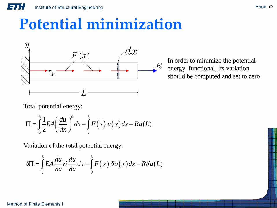
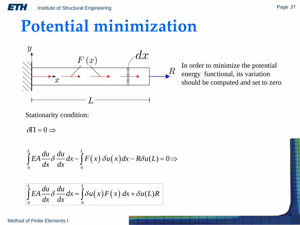
Potential minimization
Total potential energy:
Variation of the total potential energy:
2
0 0
1( )
2
L Ldu
EA dx F x u x dx Ru Ldx
In order to minimize the potential
energy functional, its variation
should be computed and set to zero
0 0
( )
L Ldu du
EA dx F x u x dx R u Ldx dx
Institute of Structural Engineering Page 31
Method of Finite Elements I
Potential minimization
Stationarity condition:
In order to minimize the potential
energy functional, its variation
should be computed and set to zero
0 0
0 0
0
( ) 0
( )
L L
L L
du duEA dx F x u x dx R u L
dx dx
du duEA dx u x F x dx u L R
dx dx
Institute of Structural Engineering Page 32
Method of Finite Elements I
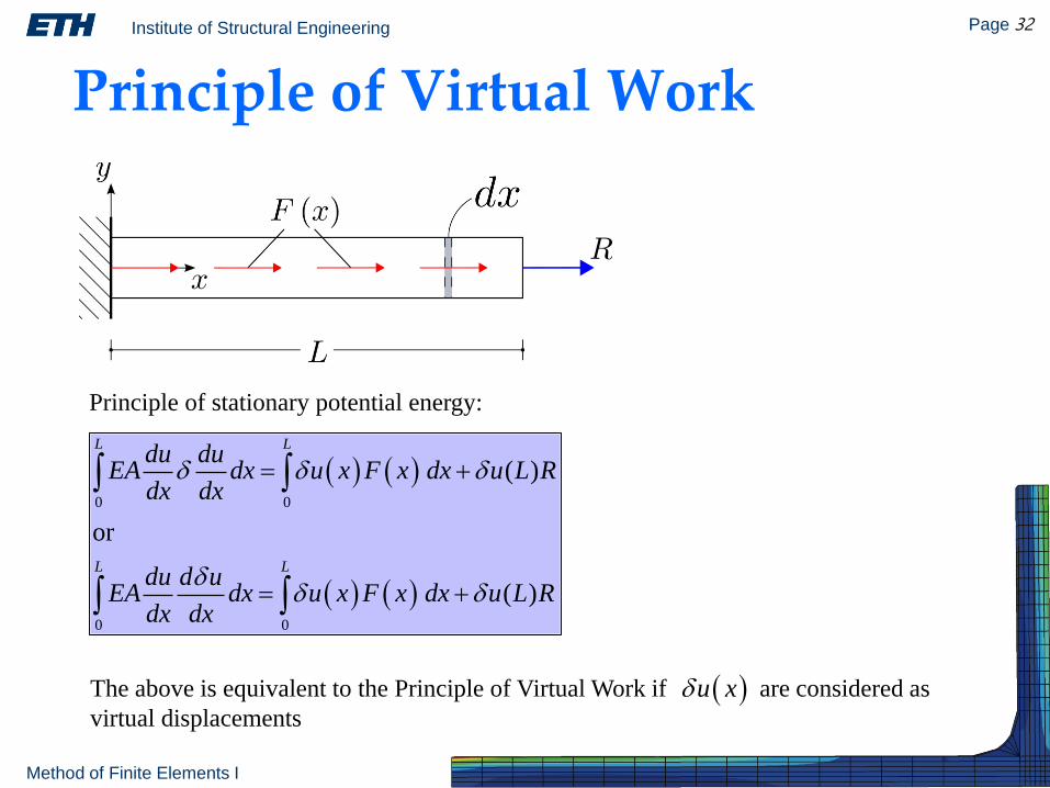
Principle of Virtual Work
Principle of stationary potential energy:
0 0
0 0
( )
or
( )
L L
L L
du duEA dx u x F x dx u L R
dx dx
du d uEA dx u x F x dx u L R
dx dx
The above is equivalent to the Principle of Virtual Work if are considered as
virtual displacements u x
Institute of Structural Engineering Page 33
Method of Finite Elements I
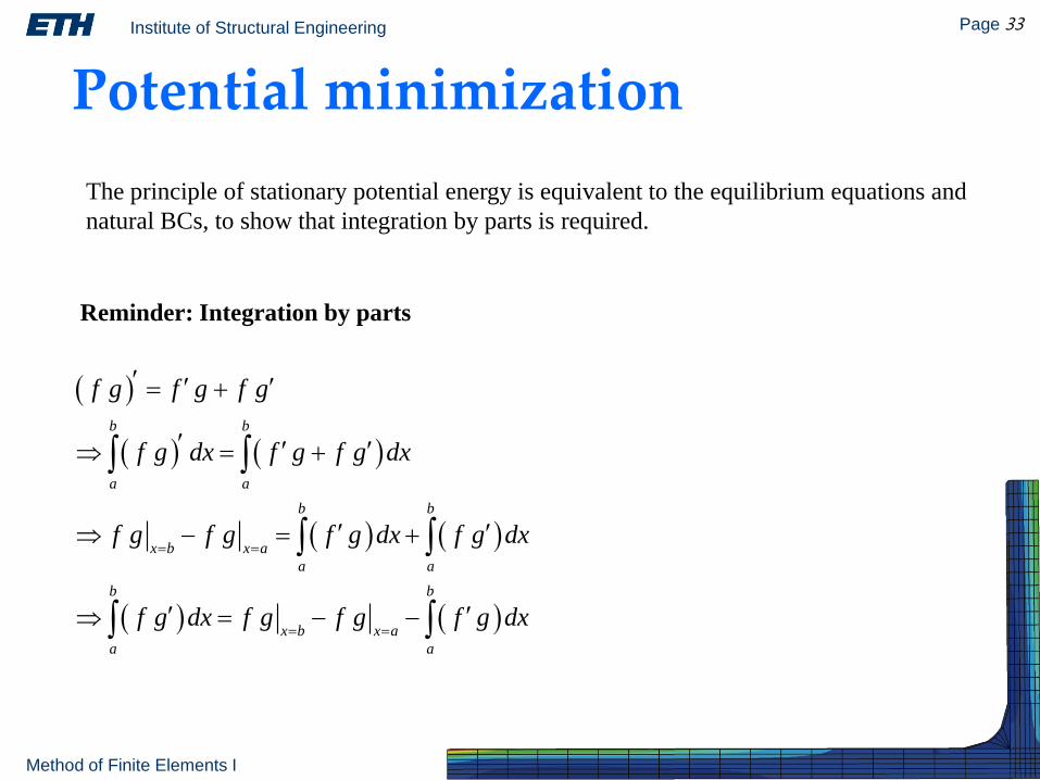
b b
a a
b b
x b x a
a a
b b
x b x a
a a
f g f g f g
f g dx f g f g dx
f g f g f g dx f g dx
f g dx f g f g f g dx
Reminder: Integration by parts
Potential minimization
The principle of stationary potential energy is equivalent to the equilibrium equations and
natural BCs, to show that integration by parts is required.

Institute of Structural Engineering Page 34
Method of Finite Elements I
Potential minimizationPrinciple of stationary potential energy:
0 0
( ) 0
L Ldu du
EA dx u x F x dx u L Rdx dx
Integration by parts for the first term:
2
2
0 0
0
0
0
L L
g g g
gf f f fx L x
x L x
du du du du d uEA dx EA u EA u EA u dx
dx dx dx dx dx
du duEA u L EA u
dx dx
2
2
0
Ld u
EA u dxdx
why?
Institute of Structural Engineering Page 35
Method of Finite Elements I
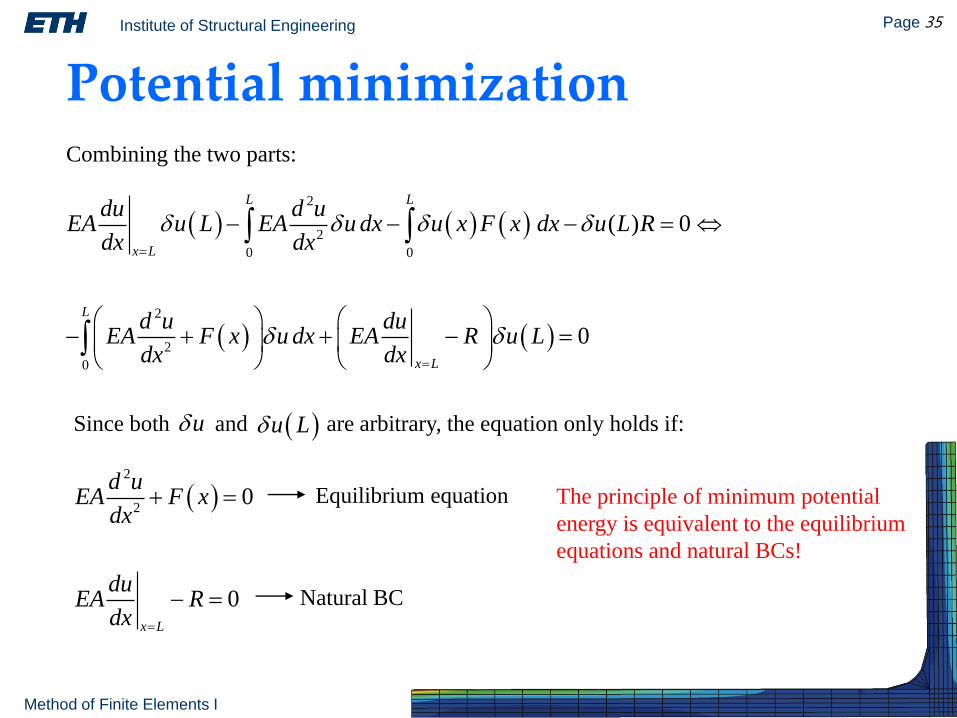
Potential minimization
2
2
0 0
2
2
0
( ) 0
0
L L
x L
L
x L
du d uEA u L EA u dx u x F x dx u L R
dx dx
d u duEA F x u dx EA R u L
dx dx
Combining the two parts:
Since both and are arbitrary, the equation only holds if:u u L
2
20
0x L
d uEA F x
dx
duEA R
dx
Equilibrium equation
Natural BC
The principle of minimum potential
energy is equivalent to the equilibrium
equations and natural BCs!
Institute of Structural Engineering Page 36
Method of Finite Elements I
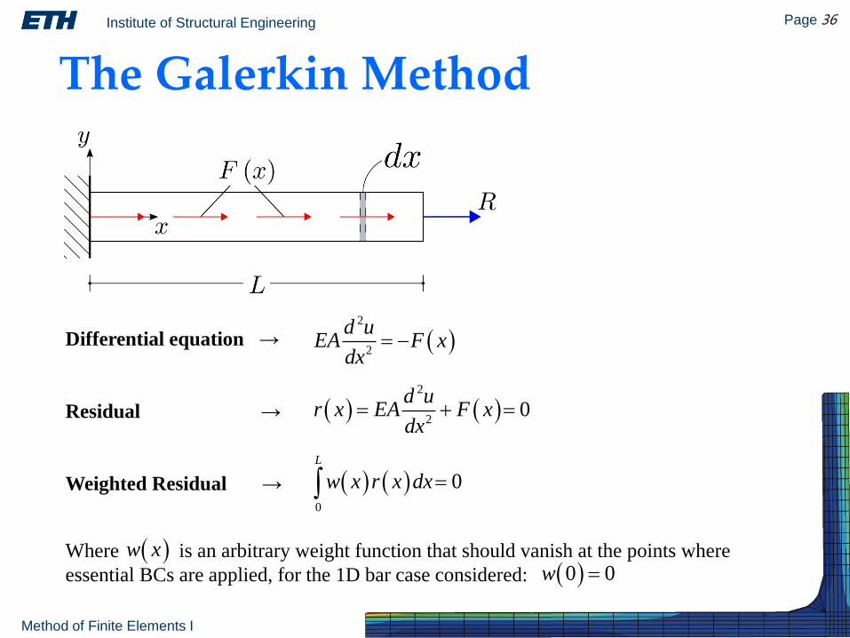
The Galerkin Method
2
2
d uEA F x
dx Differential equation →
Residual →
Weighted Residual →
2
20
d ur x EA F x
dx
0
0
L
w x r x dx
w xWhere is an arbitrary weight function that should vanish at the points where
essential BCs are applied, for the 1D bar case considered: 0 0w
Institute of Structural Engineering Page 37
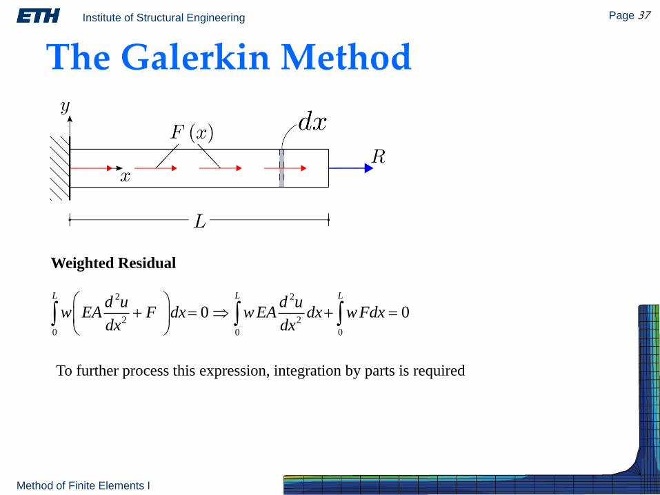
Method of Finite Elements I
2 2
2 2
0 0 0
0 0
L L Ld u d u
w EA F dx wEA dx wFdxdx dx
The Galerkin Method
Weighted Residual
To further process this expression, integration by parts is required
Institute of Structural Engineering Page 38
Method of Finite Elements I
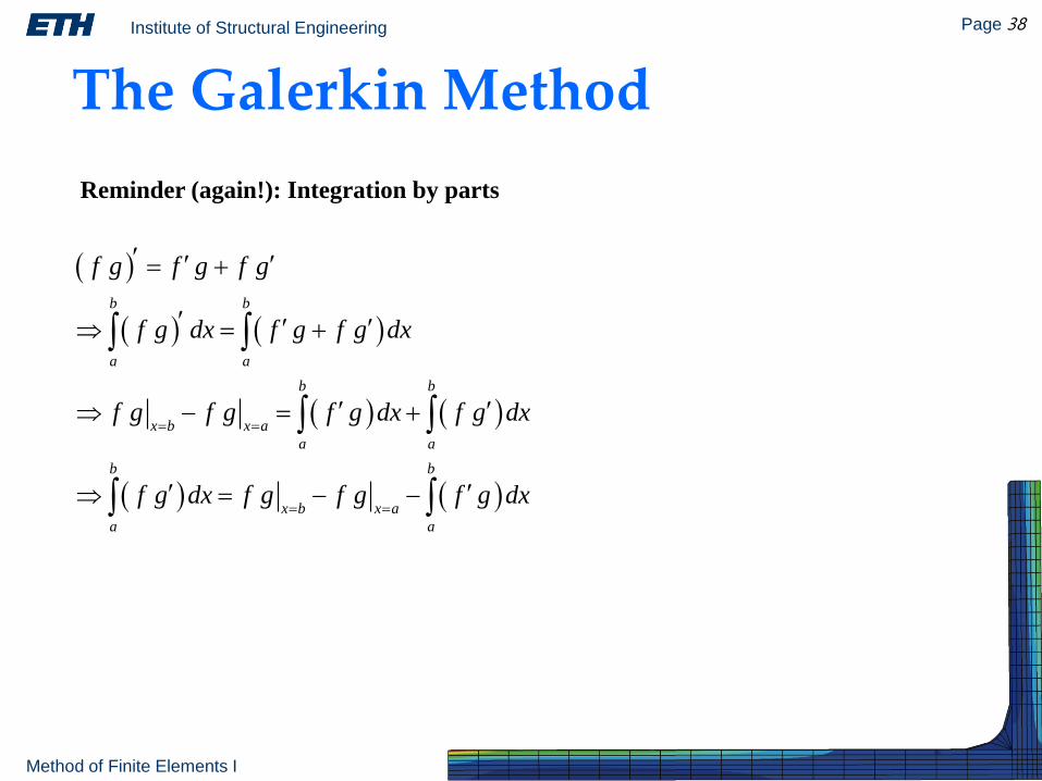
b b
a a
b b
x b x a
a a
b b
x b x a
a a
f g f g f g
f g dx f g f g dx
f g f g f g dx f g dx
f g dx f g f g f g dx
Reminder (again!): Integration by parts
The Galerkin Method
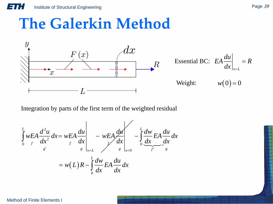
Institute of Structural Engineering Page 39
Method of Finite Elements I
2
2
0
0
L
f f f
g g gx L x
d u du duwEA dx wEA wEA
dx dx dx
0
0
L
gf
L
dw duEA dx
dx dx
dw duw L R EA dx
dx dx
The Galerkin Method
Integration by parts of the first term of the weighted residual
0 0w
x L
duEA R
dx
Essential BC:
Weight:
Institute of Structural Engineering Page 40
Method of Finite Elements I
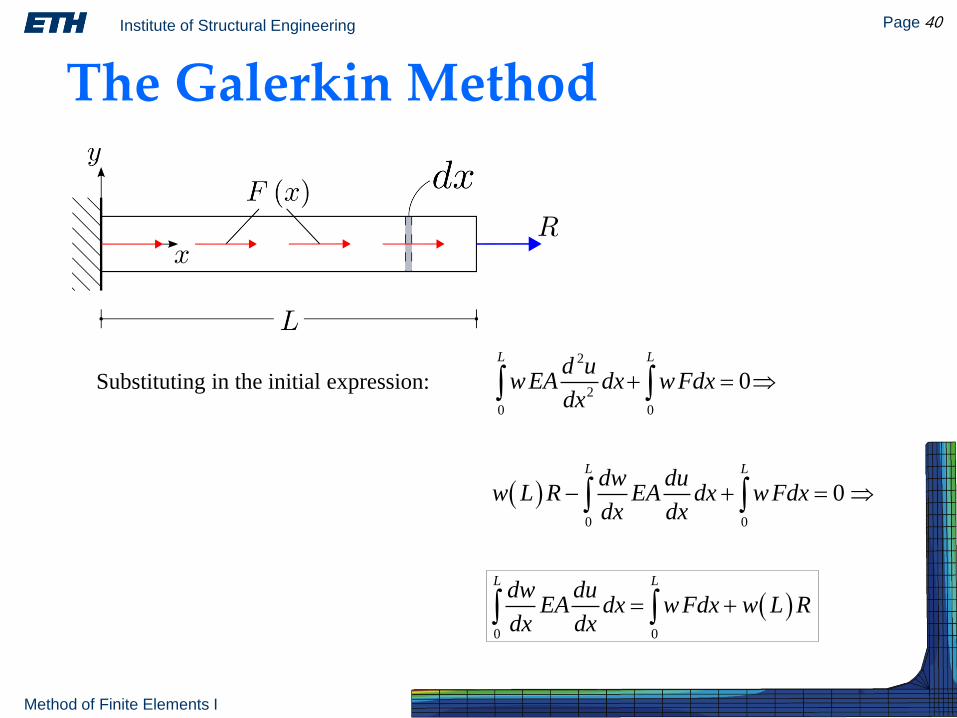
The Galerkin Method
Substituting in the initial expression:
2
2
0 0
0 0
0 0
0
0
L L
L L
L L
d uwEA dx wFdx
dx
dw duw L R EA dx wFdx
dx dx
dw duEA dx wFdx w L R
dx dx
Institute of Structural Engineering Page 41
Method of Finite Elements I
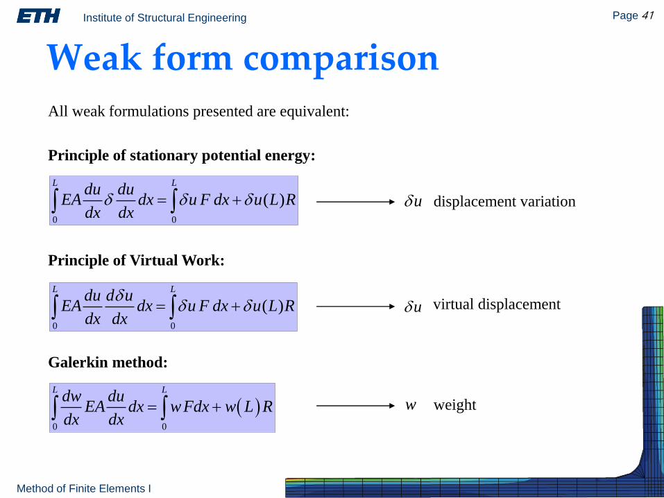
Weak form comparison
0 0
L Ldw du
EA dx wFdx w L Rdx dx
0 0
( )
L Ldu du
EA dx u F dx u L Rdx dx
0 0
( )
L Ldu d u
EA dx u F dx u L Rdx dx
Principle of stationary potential energy:
Principle of Virtual Work:
Galerkin method:
All weak formulations presented are equivalent:
u
u
w
displacement variation
virtual displacement
weight
Institute of Structural Engineering Page 42
Method of Finite Elements I
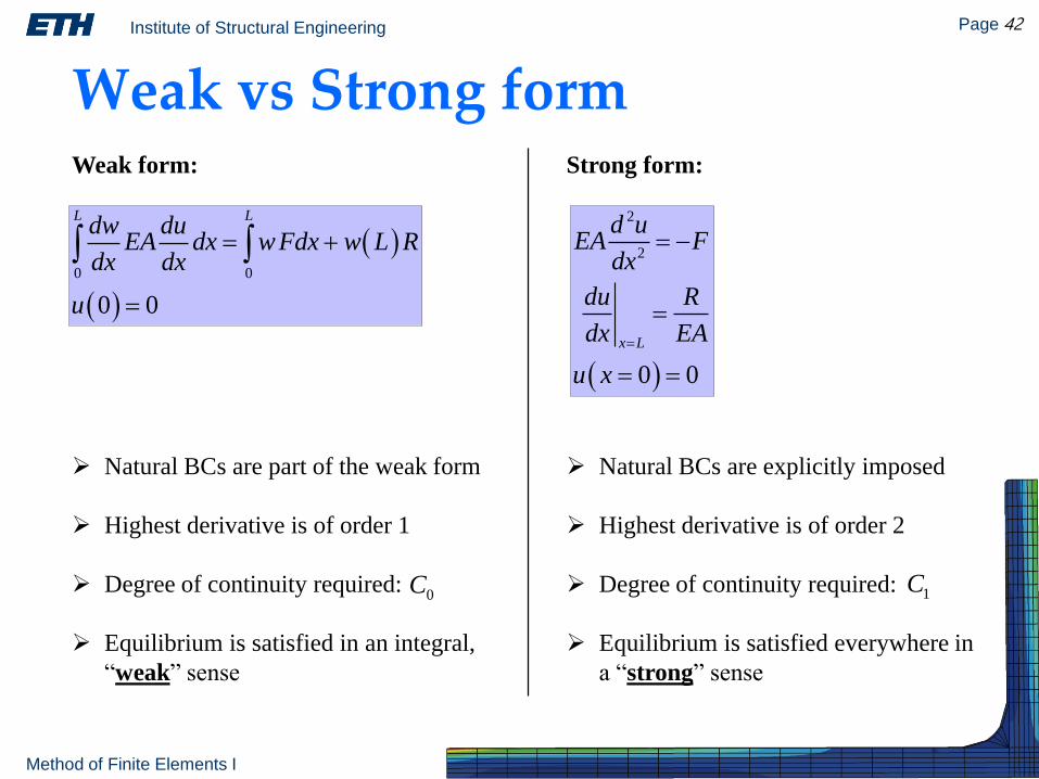
Weak vs Strong form
0 0
0 0
L Ldw du
EA dx wFdx w L Rdx dx
u
Weak form:
2
2
0 0
x L
d uEA F
dx
du R
dx EA
u x
Strong form:
Natural BCs are part of the weak form
Highest derivative is of order 1
Degree of continuity required:
Equilibrium is satisfied in an integral,
“weak” sense
Natural BCs are explicitly imposed
Highest derivative is of order 2
Degree of continuity required:
Equilibrium is satisfied everywhere in
a “strong” sense
0C 1C
Institute of Structural Engineering Page 43
Method of Finite Elements I
Weak form solution
A general process:
Assume a general form for the solution
Plug into weak form
Obtain unknown coefficients
In this process:
The problem formulation poses restrictions with respect to possible forms of the
solution
The weak form is much less restrictive than the corresponding strong form
Institute of Structural Engineering Page 44
Method of Finite Elements I
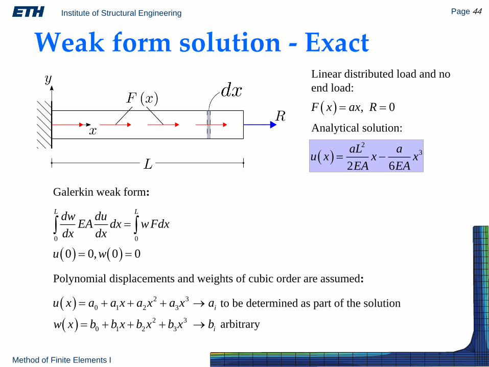
Weak form solution - ExactLinear distributed load and no
end load:
, 0F x ax R
2
3
2 6
aL au x x x
EA EA
Analytical solution:
0 0
0 0, 0 0
L Ldw du
EA dx wFdxdx dx
u w
to be determined as part of the solution
Polynomial displacements and weights of cubic order are assumed:
2 3
0 1 2 3
2 3
0 1 2 3
i
i
u x a a x a x a x a
w x b b x b x b x b
Galerkin weak form:
arbitrary
Institute of Structural Engineering Page 45
Method of Finite Elements I
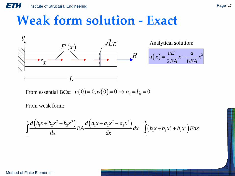
Analytical solution:
Weak form solution - Exact
2
3
2 6
aL au x x x
EA EA
From weak form:
From essential BCs: 0 00 0, 0 0 0u w a b
2 3 2 3
1 2 3 1 2 3 2 3
1 2 3
0 0
L Ld b x b x b x d a x a x a xEA dx b x b x b x Fdx
dx dx
Institute of Structural Engineering Page 46
Method of Finite Elements I
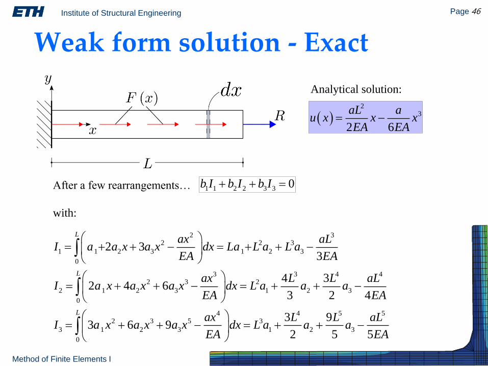
Weak form solution - Exact
After a few rearrangements…
with:
1 1 2 2 3 3 0b I b I b I
2 32 2 3
1 1 2 3 1 2 3
0
3 3 4 42 3 2
2 1 2 3 1 2 3
0
4 4 5 52 3 5 3
3 1 2 3 1 2 3
0
2 33
4 32 4 6
3 2 4
3 93 6 9
2 5 5
L
L
L
ax aLI a a x a x dx La L a L a
EA EA
ax L L aLI a x a x a x dx L a a a
EA EA
ax L L aLI a x a x a x dx L a a a
EA EA
Analytical solution:
2
3
2 6
aL au x x x
EA EA
Institute of Structural Engineering Page 47
Method of Finite Elements I
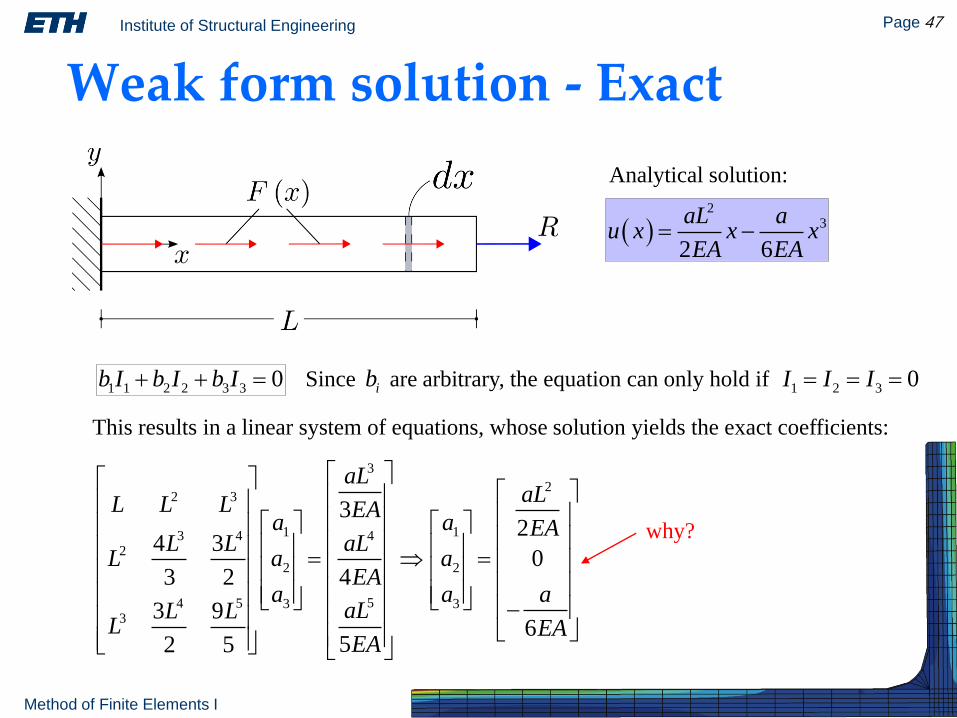
Weak form solution - Exact
Since are arbitrary, the equation can only hold if1 1 2 2 3 3 0b I b I b I ib 1 2 3 0I I I
This results in a linear system of equations, whose solution yields the exact coefficients:
3
22 3
1 13 4 42
2 2
54 5 3 33
32
4 30
3 2 4
3 96
52 5
aLaLL L L EA
a a EAL L aL
L a aEA
a a aaLL L
L EAEA
Analytical solution:
2
3
2 6
aL au x x x
EA EA
why?
Institute of Structural Engineering Page 48
Method of Finite Elements I
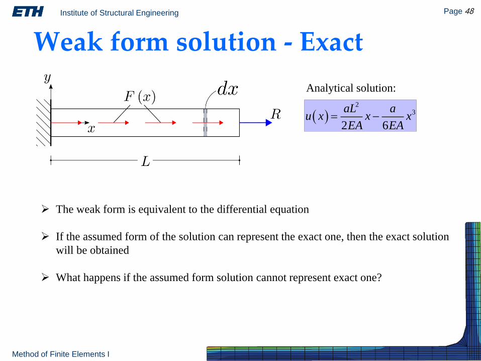
Weak form solution - Exact
Analytical solution:
2
3
2 6
aL au x x x
EA EA
The weak form is equivalent to the differential equation
If the assumed form of the solution can represent the exact one, then the exact solution
will be obtained
What happens if the assumed form solution cannot represent exact one?
Institute of Structural Engineering Page 49
Method of Finite Elements I
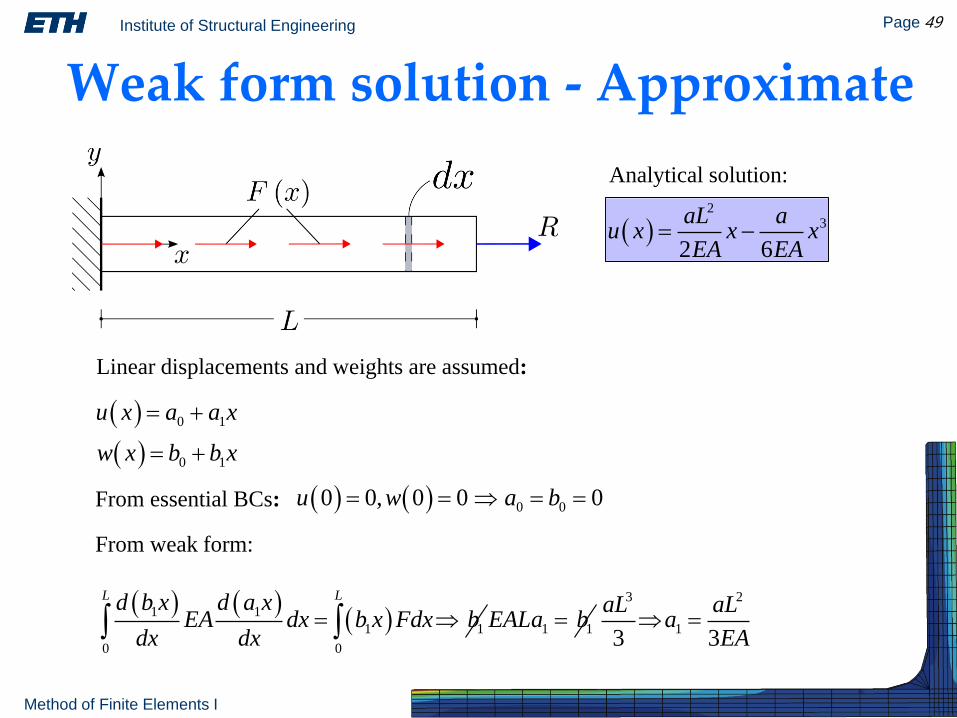
Weak form solution - Approximate
Analytical solution:
2
3
2 6
aL au x x x
EA EA
Linear displacements and weights are assumed:
0 1
0 1
u x a a x
w x b b x
From weak form:
From essential BCs: 0 00 0, 0 0 0u w a b
1 1
1 1
0 0
L Ld b x d a xEA dx b x Fdx b
dx dx 1 1EALa b
3 2
13 3
aL aLa
EA
Institute of Structural Engineering Page 50
Method of Finite Elements I
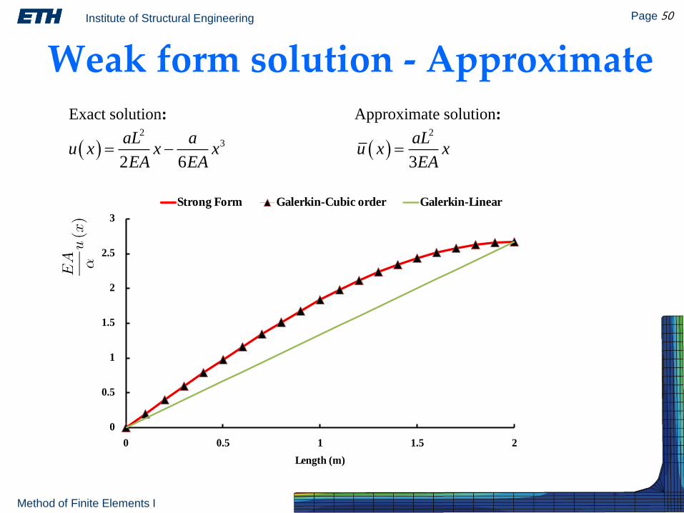
Weak form solution - ApproximateExact solution:
2
3
aLu x x
EA
23
2 6
aL au x x x
EA EA
Approximate solution:
0
0.5
1
1.5
2
2.5
3
0 0.5 1 1.5 2
Length (m)
Strong Form Galerkin-Cubic order Galerkin-Linear


![GRIFFITHS VARIATIONAL MULTISYMPLECTIC FORMULATION FOR LOVELOCK … · 2019-11-19 · arXiv:1911.07278v1 [math-ph] 17 Nov 2019 GRIFFITHS VARIATIONAL MULTISYMPLECTIC FORMULATION FOR](https://static.fdocuments.in/doc/165x107/5e8987e208730c54b21eb349/griffiths-variational-multisymplectic-formulation-for-lovelock-2019-11-19-arxiv191107278v1.jpg)