Eigenvalues of the curl operator: variational formulation and ...

IntroductionThe mathematical problem

The variational problemSpectral analysis

Finite element approximationNumerical results

Eigenvalues of the curl operator:variational formulation and numerical

approximation

Alberto Valli

Dipartimento di Matematica, Universita di Trento, Italy

A. Valli Eigenvalus of the curl




Joint paper with:

Ana Alonso RodrıguezDipartimento di Matematica, Universita di Trento, Italy

Jessika CamanoDepartamento de Matematica y Fısica Aplicadas, UniversidadCatolica de la Santısima Concepcion, Chile

Rodolfo RodrıguezDepartamento de Ingenierıa Matematica, Universidadde Concepcion, Chile

Pablo VenegasDepartamento de Matematica, Universidad del Bıo Bıo, Chile





Outline

1 Introduction

2 The mathematical problem

3 The variational problem

4 Spectral analysis

5 Finite element approximation

6 Numerical results





Introduction





Physical framework

By the Lorentz law the density of the magnetic force is given byF = J× B, where J is the current density and B is the magneticinduction.

Linear isotropic media: B = µH (the scalar function µ beingthe magnetic permeability).

Eddy current or static approximation: J = curl H.

If curl H = λH (λ a scalar function) the magnetic force vanishes:

F = curl H× µH = λH× µH = 0 .





Physical framework (cont’d)

Fields satisfying curl H = λH are called force-free fields. If λis a constant are called linear force-free fields.

[Clearly, the most interesting case is for λ not identically vanishing.]

[In fluid dynamics, force-free fields are called Beltrami fields, and aBeltrami field u that is divergence-free and tangential to theboundary is a steady solution of the Euler equations forincompressible inviscid flows (with pressure given by p = −|u|2/2).]





Physical framework (cont’d)

A couple of interesting physical remarks:

a field which is divergence-free and tangential to the boundary(e.g., the magnetic field), and which minimizes the magneticenergy with fixed helicity is a linear force-free field [Woltjer(1958)];

linear force-free fields are time-asymptotic configurations(they remain force-free as time changes) [Jette (1970)].

[Helicity of a vector field v in a domain Ω, i.e.,

H(v) =1

4π

∫Ω

∫Ω

v(x)× v(y) · x− y

|x− y|3dxdy ,

is a “measure of the extent to which the field lines wrap and coilaround one another” (Cantarella et al. (2000:a); other physicalremarks can be found there and in Cantarella et al. (2000:b)).]





The mathematical problem





Mathematical framework

Let us focus now on the mathematical aspects of this problem.

A linear force-free field is an eigenfunction of the curl operator:

curl u = λu .

It is thus interesting to see when it is possible to define self-adjointrealizations of the curl operator. The starting point is clearly theGreen’s formula (here and in the sequel we write Γ = ∂Ω)∫

Ω(v · curl w − curl v ·w) =

∫Γ

v × n ·w ,

and the analysis is driven by the need of obtaining∫

Γ v× n ·w = 0.





The spectral problem: Ω simply-connected

It is clear that∫

Γ v × n ·w = 0 when v × n = 0 on Γ. However,this boundary condition is too strong for the spectral problem.

Weaker boundary conditions can be devised (see, e.g., Kress (1972,1986); Picard (1976, 1998); Yoshida and Giga (1990)).

When Ω is a simply-connected domain, it is sufficient to assumethat curl v · n = 0 on Γ. Since for an eigenfunction u of the curloperator the condition u · n = 0 implies curl u · n = 0, it is thusnatural to consider the spectral problem

curl u = λu in Ωdiv u = 0 in Ωu · n = 0 on Γ .

(1)

The numerical approximation of (1) has been analyzed inRodrıguez and Venegas (2014).





The spectral problem: Ω not simply-connected

The condition curl v · n = 0 is not enough if the physical domain isnot simply-connected.

A possible additional condition is the following (see, e.g., Kress(1972, 1986); Picard (1976, 1998); Yoshida and Giga (1990)): thecurl operator is self-adjoint if curl v · n = 0 on Γ (which isequivalent to curl v⊥∇H1(Ω)) and curl v⊥KT , where KT is thespace of the so-called harmonic Neumann fields h (those fieldssatisfying curl h = 0 in Ω, div h = 0 in Ω and h · n = 0 on Γ).This space KT is finite dimensional, its dimension being the firstBetti number of Ω; it is trivial for a simply-connected domain Ω.

It can be proved that H0(curl; Ω) = ∇H1(Ω)⊥⊕ KT .

The numerical approximation of the eigenvalues and eigenfunctionsof this problem has been studied in Lara et al. (2016).





The spectral problem: Ω not simply-connected (cont’d)

It is worth noting that the condition curl v⊥KT is not essential,but only sufficient for the proof that the curl operator isself-adjoint.

In this respect, an in-depth analysis has been recently presented inHiptmair et al. (2012). The authors, by incorporating in problem(1) additional conditions related to the first homology group of Γ,devise suitable self-adjoint realizations of the curl operator.





Homological tools

Let us show how this family of eigenvalue problems can bedescribed.We first need to recall some geometrical results. Let g be the firstBetti number Ω; then the first Betti number of Γ is equal to 2g .From algebraic topology we know that:

on Γ there are 2g non-bounding cycles γjgj=1 ∪ γ′jgj=1, that

are the generators of the first homology group of Γ

γjgj=1 are the generators of the first homology group of Ω′,

with Ω′ = B \ Ω, B being an open ball containing Ω (tangentvector on γj denoted by tj);

γ′jgj=1 are the generators of the first homology group of Ω

(tangent vector on γ′j denoted by t′j);





Homological tools (cont’d)

in Ω there exist g ‘cutting’ surfaces Σjgj=1, that areconnected orientable Lipschitz surfaces satisfying Σj ⊂ Ω and∂Σj ⊂ Γ, such that every curl-free vector in Ω has a globalpotential in the ‘cut’ domain Ω0 := Ω \

⋃gj=1 Σj ; each surface

Σj satisfies ∂Σj = γj , ‘cuts’ the corresponding cycle γ′j anddoes not intersect the other cycles γ′i for i 6= j ;

in Ω′ there exist g ‘cutting’ surfaces Σ′jgj=1, that are

connected orientable Lipschitz surfaces satisfying Σ′j ⊂ Ω′ and∂Σ′j ⊂ Γ, such that every curl-free vector in Ω′ has a global

potential in the ‘cut’ domain (Ω′)0 := Ω′ \⋃g

j=1 Σ′j ; eachsurface Σ′j satisfies ∂Σ′j = γ′j , ‘cuts’ the corresponding cycleγj , and does not intersect the other cycles γi for i 6= j .





Homological tools (cont’d)

[Some misunderstanding appears when looking back at theliterature on this topic; it is thus interesting to make clear that:

the statement concerning the ‘cutting’ surfaces Σj does notmean that the ‘cut’ domain Ω0 is simply-connected nor that itis homologically trivial: an example in this sense is furnishedby Ω = Q \ K , where Q is a cube and K is the trefoil knot.]





A typical geometrical situation

Figure: Toroidal domain. Σ1 and Σ′1 represent the ’cutting’ surfaces of Ω

and Ω′, respectively.





New homological conditions

Hiptmair et al. (2012), have shown that the curl operator isself-adjoint in the space of vector fields v with curl v · n = 0 on Γand such that

∮γi

v · ti = 0 for 1 ≤ i ≤ g1 and∮γ′j

v · t′j = 0 for

g1 + 1 ≤ j ≤ g , where g1 is a fixed number satisfying 0 ≤ g1 ≤ g .

If curl v · n = 0 on Γ the choice g1 = g , namely,∮γi

v · ti = 0for 1 ≤ i ≤ g1 = g , is equivalent to the previous conditioncurl v⊥KT [we wll return on this point in the sequel].





New homological conditions (cont’d)

However,

the most interesting physical case is the one given by thechoice g1 = 0, i.e., the additional conditions are given by∮γ′j

v · t′j = 0 for 1 ≤ j ≤ g .

In fact, in this case the eigenfunction associated to the eigenvalueof minimum absolute value realizes the minimum of the magneticenergy with fixed helicity.





The eigenvalue problem

Summing up, we consider the following eigenvalue problem:

Problem 1. Find λ ∈ C and u ∈ L2(Ω)3, u 6= 0, such that

curl u = λu in Ω

divu = 0 in Ω

u · n = 0 on Γ∮γi

u · ti = 0 1 ≤ i ≤ g1∮γ′j

u · t′j = 0 g1 + 1 ≤ j ≤ g ,

(2)

where 0 ≤ g1 ≤ g .





A basis for KT

A basis of the space KT is given byρj

gj=1

, where ρj = ∇φj (the

L2(Ω)3-extension of ∇φj), and φj is the unique solution of

∆φj = 0 in Ω \ Σj ,∂nφj = 0 on ∂Ω ,[[ ∂nφj ]]Σj

= 0 ,

[[φj ]]Σj= 1 .

In a similar way we construct a basisρ′j

g

j=1of the space of

harmonic Neumann vector fields K′T associated to the domainΩ′ = B \ Ω.





The meaning of the line integrals

By the Stokes theorem and integration by parts we can see thatthe meaning of the line integrals is:∮

γiu · ti =

∫Σi

curl u · ni =∫

Σicurl u · ni [[φi ]]Σi

=∫

Ω\Σicurl u · ∇φi =

∫Ω curl u · ∇φi

=∫

Ω curl u · ρi =∫

Γ n× u · ρi ,

and similarly ∮γ′j

u · t′j = −∫

Γ n× u · ρ′j .





The “orthogonality” relations

In particular, the fundamental “orthogonality” relations∮γiρs · ti =

∫Γ n× ρs · ρi = 0∮

γ′jρ′s · t′j = −

∫Γ n× ρ′s · ρ′j = 0∮

γ′iρs · t′i = −

∫Γ n× ρs · ρ′i = δs,i∮

γjρ′s · tj =

∫Γ n× ρ′s · ρj = δs,j

(3)

hold true, together with∮γi∇ω · ti =

∫Γ n×∇ω · ρi = 0∮

γ′j∇ω · t′j = −

∫Γ n×∇ω · ρ′j = 0 .

(4)





The variational problem





Variational formulation

Some function spaces:

X = v ∈ H(curl; Ω) : curl v · n = 0 on Γ ,

X 0 = v ∈ X :∮γi

v · ti = 0 for i = 1, . . . , g1 ,

X ? = v ∈ X :∮γ′j

v · t′j = 0 for j = g1 + 1, . . . , g ,

Z = X 0 ∩X ? ,

Q = ∇H1(Ω)⊕ span ρ1, . . . ,ρg1 .

The following equality holds trueQ = X ? ∩ H(curl 0; Ω) = Z ∩ H(curl 0; Ω) . (5)

(for the second equality, the key point is that the cycles γi arebounding in Ω!).





Variational formulation (cont’d)

A saddle-point formulation of Problem 1 is devised by looking for avector field u in Z and a Lagrange multiplier q (associated to thedivergence-free and boundary constraints) in Q. It reads:

Problem 2. Find λ ∈ C and (u,q) ∈ Z ×Q, u 6= 0, such that∫Ω

curl u · curl v +

∫Ω

q · v = λ

∫Ω

u · curl v ∀ v ∈ Z (6a)∫Ω

u · p = 0 ∀p ∈Q . (6b)





Variational formulation (cont’d)

It is worth noting that the Lagrange multiplier q in Problem 2is vanishing. Moreover, an eigenvalue λ must be differentfrom 0.

In fact, taking v = q ∈Q ⊂ Z in (6a) it follows q = 0. Hence, ifwe suppose λ = 0, we obtain curl u = 0 in Ω, and consequentlyu ∈Q by equality (5). Choosing p = u in (6b) it follows u = 0,and we conclude that λ = 0 is not admissible.





Equivalence of the eigenvalue problems

Lemma

If (λ,u), λ 6= 0, is a solution to Problem 1, then (λ,u, 0) is asolution to Problem 2. If (λ,u,q) is a solution to Problem 2, thenq = 0 and (λ,u) is a solution to Problem 1.





Equivalence of the eigenvalue problems (cont’d)

From Problem 1 to Problem 2

If (λ,u), λ 6= 0, is a solution to Problem 1, then clearly (6a) issatisfied with q = 0. Since u ∈ H0(div 0; Ω), it follows that u isorthogonal to the gradients. Therefore, recalling that p ∈Q canbe written as p = ∇ψ +

∑g1

i=1 αiρi , we have only to prove that∫Ω u · ρi = 0 for i = 1, . . . , g1. We have already seen that∮

γiu · ti =

∫Ω curl u · ρi ,

hence the condition∮γi

u · ti = 0 can be interpreted as

λ∫

Ω u · ρi = 0, and the thesis follows because λ 6= 0. 2

[Here we have also seen that∮γi

u · ti = 0 for each i = 1, . . . , g

means curl u⊥KT ...]A. Valli Eigenvalus of the curl





From Problem 2 to Problem 1

If (λ,u,q) is a solution to Problem 2, we have already seen thatq = 0. Moreover, taking in (6b) p ∈ ∇H1(Ω) ⊂Q it followsdivu = 0 in Ω and u · n = 0 on Γ. Therefore, we only need toprove that curl u = λu in Ω.By integrating by parts (6a) we find curl(curl u− λu) = 0 in Ωand ∫

Γ(curl u− λu) · n× v = 0 (7)

for each v ∈ Z.We know that curl u− λu = ∇ϕ+

∑gs=1 βsρs , as curl u− λu is

curl-free. Moreover, for v ∈ Z we have on Γ

n× v = n× (∇ω +

g1∑k=1

ζkρk +

g∑l=g1+1

ηlρ′l) .






Thus, using the “orthogonality” relations (3) and (4) for ρi andρ′j , it follows that curl u− λu = ∇ϕ+

∑g1

i=1 βiρi ∈Q.

Therefore by (6b) u is orthogonal to λu− curl u and we have

0 =∫

Ω λu · (λu− curl u)

=∫

Ω(λu− curl u) · (λu− curl u)

+∫

Ω curl u · (λu− curl u) .

The last integral vanishes due to (6a), thus it follows curl u = λuin Ω. 2





Spectral analysis





The solution operator

In order to obtain a spectral characterization of Problem 2 weintroduce the following solution operator:

T : Z −→ Z ,f 7−→ Tf := w ,

where (w,q) ∈ Z ×Q is the solution of∫Ω

curl w · curl v +

∫Ω

q · v =

∫Ω

f · curl v ∀ v ∈ Z (8a)∫Ω

w · p = 0 ∀p ∈Q . (8b)





The solution operator: well-posedness

The well-posedness of T follows by these three lemmas.

Lemma (Poincare)

The seminorm

‖|w‖| =‖curl w‖2

0,Ω + ‖divw‖20,Ω +

∑g1

i=1

∣∣∫Ω w · ρi

∣∣2+∑g

j=g1+1

∣∣∣∮γ′j w · t′j∣∣∣2 1/2

is equivalent to the norm in X ∩ H0(div ; Ω).

Proof. By contradiction, in a somehow standard way. The mainpoint is showing that a harmonic Neumann field w with∑g1

i=1

∣∣∫Ω w · ρi

∣∣2 = 0 and∑g

j=g1+1

∣∣∣∮γ′j w · t′j∣∣∣2 = 0 is null. 2





The solution operator: well-posedness (cont’d)

Lemma (ellipticity in the kernel)

There exists α > 0 such that∫Ω|curl v|2 ≥ α‖v‖2

curl,Ω ∀v ∈ V ,

where

V =

v ∈ Z :

∫Ω

v · p = 0 ∀p ∈Q.

Proof. By the Poincare lemma, as an element v ∈ V satisfiesdiv v = 0 in Ω, v · n = 0 on Γ,

∫Ω w · ρi = 0 for i = 1, . . . , g1 (as it

is orthogonal to Q) and∮γ′j

w · t′j = 0 for j = g1 + 1, . . . , g (as it

belongs to Z). 2





The solution operator: well-posedness (cont’d)

Lemma (inf–sup condition)

There exists β > 0 such that

supv∈Z,v 6=0

∣∣∫Ω v · p

∣∣‖v‖curl,Ω

≥ β ‖p‖0,Ω ∀p ∈ Q .

Proof. Just take v = p ∈Q ⊂ Z, and note that curl v = 0. 2

Thus problem (8) is well-posed (Babuska–Brezzi theory forsaddle-point problems).





Looking for the eigenvalues of T

We have that Tu = µu, with µ 6= 0, if and only if (λ,u, 0) is asolution of Problem 2, with λ = 1/µ.

We thus focus on the spectrum of T. The following result is easilyproved:

Lemma

The Lagrange multiplier q in (8a) is null

Tf ∈ H(curl; Ω) ∩ H0(div 0; Ω) andcurl Tf ∈ H(curl; Ω) ∩ H0(div 0; Ω)

T is compact

(curl Tf − f) ∈Q.





Symmetry of the curl operator

For the analysis of the spectral problem the fundamental theoremis:

Theorem (Symmetry of the curl)

For all v, w ∈ Z, ∫Ω

(curl w · v −w · curl v) = 0.





Symmetry of the curl operator (cont’d)

Proof. Since∫Ω

curl w · v −∫

Ωw · curl v =

∫Γ(n×w) · v ,

the point is to show that∫

Γ(n×w) · v = 0. Recall that w ∈ Z canbe written on Γ as

n×w = n× (∇ω +

g1∑k=1

ζkρk +

g∑l=g1+1

ηlρ′l) ,

and analogously v ∈ Z. Moreover it is easily proved that∫Γ(n×∇ω) · ∇θ =

∫Ω

(curl∇ω) · ∇θ = 0 .

Hence, using the orthogonality relations (3) and (4), the resultfollows at once. 2





Self-adjointness of the operator T

The symmetry of the curl operator has this easy but pivotalconsequence:

Theorem

The operator T : Z → Z is self-adjoint.





Self-adjointness of the operator T (cont’d)

Proof. We know that (curl Tf − f) and (curl Tg − g) belong toQ. Since Tf, Tg satisfy (8b) we have that∫

Ω Tf · g =∫

Ω Tf · g +∫

Ω Tf · (curl Tg − g)

=∫

Ω Tf · curl Tg =∫

Ω curl Tf · Tg

=∫

Ω(f − curl Tf) · Tg +∫

Ω curl Tf · Tg

=∫

Ω f · Tg ,

having used the symmetry of the curl operator in Z.On the other hand, from (8a) and the symmetry again, we obtain∫

Ω curl Tf · curl g =∫

Ω f · curl g =∫

Ω curl f · g

=∫

Ω curl f · curl Tg ,

which ends the proof. 2





Spectral analysis of the operator T

We are now in a position to obtain a spectral characterization of T.

Theorem

The spectrum of T is given by sp(T)=0 ∪ µn∞n=1, where

µ0 = 0 is an infinite-multiplicity eigenvalue (and its associatedeigenspace is Q)

µn∞n=1 is a sequence of finite-multiplicity eigenvalues whichconverges to 0 and the associated eigenfunctions un∞n=1 area Hilbertian basis of Z.





Spectral analysis of the operator T (cont’d)

Proof. The spectral result is classical; we only need to prove thatKerT=Q. We easily have

KerT =

f ∈ Z :

∫Ω

f · curl v = 0 ∀ v ∈ Z⊂Q .

Conversely, f ∈Q ⊂ Z satisfies curl f = 0 in Ω, thus by thesymmetry of the curl operator for all v ∈ Z it holds∫

Ω f · curl v =∫

Ω curl f · v = 0. 2





Finite element approximation





Nedelec finite elements

We consider a family of triangulations Th of the polyhedral domainΩ. For k ≥ 1 and T ∈ Th

Pk is the set of polynomials of degree not greater than k

Pk is the subset of homogeneous polynomials of degree k

N k(T ) = Pk−1(T )3 ⊕ p ∈ Pk(T )3 : p(x) · x = 0.The corresponding global space to approximate H(curl; Ω) is thewell-known Nedelec finite element space:

N kh = vh ∈ H(curl; Ω) : vh ∈ N k(T ) ∀T ∈ Th.





Discrete spaces

Whence, the natural approximation space for Z is

Zh = Z ∩N kh ,

namely,

Zh = vh ∈ N kh : curl vh · n = 0 on Γ,∮

γivh · ti = 0 for i = 1, . . . , g1∮

γ′jvh · t′j = 0 for j = g1 + 1, . . . , g .





Discrete spaces (cont’d)

To discretize the Lagrange multiplier q ∈Q we use the finiteelement space

Qh = Zh ∩ H(curl 0; Ω) .

Note that

Qh = vh ∈ N kh : curl vh = 0 in Ω,∮

γ′jvh · t′j = 0 , for j = g1 + 1, . . . , g ,

since the cycles γi are bounding in Ω and therefore a curl-freevector field has vanishing line integral on them.





The discrete problem

We are now in position to introduce a finite element discretizationof Problem 2.

Problem 3. Find λh ∈ C and (uh,qh) ∈ Zh ×Qh, uh 6= 0, suchthat∫

Ωcurl uh · curl vh +

∫Ω

qh · vh = λh

∫Ω

uh · curl vh ∀ vh ∈ Zh∫Ω

uh · ph = 0 ∀ph ∈Qh .

As for the continuous problem we have that the Lagrangemultiplier qh is null and that the eigenvalues satisfy λh 6= 0.





The discrete solution operator

We also consider the corresponding discrete solution operator:

Th : Z −→ Z ,f 7−→ Thf := wh ,

where (wh,qh) ∈ Zh ×Qh is the solution of

∫Ω

curl wh · curl vh +

∫Ω

qh · vh =

∫Ω

f · curl vh ∀ vh ∈ Zh∫Ω

wh · ph = 0 ∀ph ∈Qh .





The discrete solution operator: well-posedness

We need to satisfy the Babuska–Brezzi conditions.

Lemma (discrete ellipticity in the kernel)

There exists α > 0, independent of h, such that∫Ω|curl vh|2 ≥ α‖vh‖2

curl,Ω ∀vh ∈ Vh,

where

Vh =

vh ∈ Zh :

∫Ω

vh · ph = 0 ∀ph ∈Qh

.

Proof. More technical than in the continuous case, but along awell-established path. 2





The discrete solution operator: well-posedness (cont’d)

Lemma (discrete inf-sup condition)

There exists β > 0, independent of h, such that

supvh∈Zh,vh 6=0

∣∣∫Ω vh · ph

∣∣‖vh‖curl;Ω

≥ β ‖ph‖0,Ω , ∀ph ∈ Qh.

Proof. As in the continuous case, the inf–sup condition is easilychecked by taking vh = ph ∈Qh ⊂ Zh. 2





Convergence of the solution operators

The classical theory for compact operators can be used to provethat the eigenvalues and eigenfunctions of Problem 2 arewell-approximated by those of Problem 3. To this aim, afundamental result is:

Lemma (Convergence in norm)

There exists C > 0, independent of h, such that for all f ∈ Z

‖(T− Th)f‖curl;Ω ≤ Chmins,k‖f‖curl;Ω .

Proof. For f ∈ Z we have that Tf ∈ H(curl; Ω) ∩ H0(div 0; Ω)and curl Tf ∈ H(curl; Ω) ∩ H0(div 0; Ω); hence it is enough to usea Cea-type estimate and the fact that the Lagrange multipliersvanish. 2





Convergence results

The convergence results are:

let λ be an eigenvalue of Problem 2 with multiplicity m andE ⊂ Z the corresponding eigenspace; then, there exist exactly

m eigenvalues λ(1)h , . . . , λ

(m)h of Problem 3 which converge to

λ as h→ 0

let Eh be the direct sum of the eigenspaces corresponding to

λ(1)h , ..., λ

(m)h ; then δ(E,Eh)→ 0 as h→ 0, where

δ(E,Eh) := maxδ(E,Eh), δ(Eh,E) ,

with δ(M,N) := sup x∈M‖x‖=1

dist(x ,N).





Error estimates

The following error estimates hold true:

Theorem

Let r > 0 be such that E ⊂ H r (curl; Ω). There exist constantsC1, C2 > 0, independents of h, such that, for small h,

δ(E,Eh) ≤ C1hminr ,k , (9)

and|λ− λ(i)

h | ≤ C2h2 minr ,k, i = 1, ...,m . (10)





Numerical results





Test 1: Domain with first Betti number g = 1 and g1 = 1.

Ω is a toroidal domain of rectangular cross section0.005 ≤ R ≤ 1 and −1/2 ≤ z ≤ 1/2

the least positive eigenvalue is λ ≈ 1.73457π ≈ 5.449 (ofmultiplicity 2) [Morse (2007)]

we use the lowest-order Nedelec elements N 1h on tetrahedra.





Nh λh,1 λh,2

10286 5.624 5.62518993 5.562 5.56438304 5.517 5.51860758 5.500 5.500λext 5.452 5.449

order 2.12 2.12

λ 5.449 5.449

Table: Test 1. Smallest positive eigenvalues computed on differentmeshes.





Test 2: Domain with first Betti number g = 1 and g1 = 0.

Ω as in the Figure below (r1 = 1 and r2 = 0.5)

no analytical solution is available

we use the lowest-order Nedelec elements N 1h on tetrahedra.

Figure: Test 2. Half of the toroidal domain for the numerical test.





Nh λh,1 λh,2 λh,3 λh,4 λh,5

15554 5.066 6.633 6.636 6.710 6.71633901 4.986 6.438 6.441 6.505 6.50665720 4.958 6.372 6.376 6.432 6.433

129187 4.931 6.311 6.312 6.367 6.368195745 4.919 6.282 6.282 6.336 6.336247239 4.915 6.272 6.272 6.326 6.326λext 4.896 6.231 6.228 6.280 6.281

order 2.22 2.31 2.25 2.28 2.31

Table: Test 2. Smallest positive eigenvalues computed on differentmeshes.





104

105

106

102

101

100

err

or

N

Error

Fitted linear model

Figure: Test 2. Error curve for the smallest positive eigenvalue: loglogplot of the computed error |λh,1 − λext| versus the number of tetrahedraNh.





Figure: Test 2. Beltrami field corresponding to the smallest positiveeigenvalue.





A remark:

except for the smallest eigenvalue λh,1, the eigenvalues aresimilar to those computed by Lara et al. (2016) for the caseg = 1 and g1 = 1

the smallest eigenvalue is the most interesting one from thephysical point of view, as the associated eigenfunction realizesthe minimum of the magnetic energy with fixed helicity.





Test 3: Domain with first Betti number g = 2 and different valuesof g1.

Ω as in the Figure below

no analytical solution is available

we use the lowest–order Nedelec elements on hexahedra.

Figure: Test 3. Two-fold toroidal domain for the numerical test.





Nh λh,1 λh,2 λh,3 λh,4 λh,5 λh,6 λh,7

1280 9.345 9.456 11.471 11.559 12.209 12.238 12.4144320 8.946 9.047 10.784 10.843 11.406 11.423 11.568

10240 8.815 8.912 10.561 10.611 11.149 11.162 11.29720000 8.756 8.851 10.460 10.506 11.033 11.044 11.17534560 8.724 8.819 10.406 10.449 10.971 10.981 11.110λext 8.658 8.754 10.297 10.342 10.850 10.858 10.988

order 2.13 2.16 2.16 2.19 2.19 2.19 2.22

Table: Test 3. Smallest positive eigenvalues computed on differentmeshes for the problem corresponding to the case g = 2, g1 = 0.





103

104

10510

2

101

100

101

err

or

N

Fitted linear model

Error

Fitted linear model

Error

Fitted linear model

Error

Figure: Test 3. Error curve for the three smallest positive eigenvalue forthe problem corresponding to the case g = 2, g1 = 0: loglog plot of thecomputed error |λh,1 − λext| versus the number of hexahedra Nh.





Nh λh,1 λh,2 λh,3 λh,4 λh,5 λh,6

1280 9.412 11.465 11.559 12.206 12.234 12.4144320 9.007 10.779 10.843 11.403 11.421 11.568

10240 8.874 10.557 10.611 11.146 11.160 11.29720000 8.814 10.456 10.506 11.030 11.043 11.17534560 8.781 10.402 10.449 10.968 10.980 11.110λext 8.714 10.293 10.342 10.846 10.857 10.988

order 2.13 2.16 2.19 2.19 2.19 2.22

Table: Test 3. Smallest positive eigenvalues computed on differentmeshes for the problem corresponding to the case g = 2, g1 = 1.





Nh λh,1 λh,2 λh,3 λh,4 λh,5

1280 11.462 11.559 12.203 12.230 12.4144320 10.776 10.843 11.399 11.419 11.568

10240 10.554 10.611 11.141 11.159 11.29720000 10.454 10.506 11.025 11.042 11.17534560 10.399 10.449 10.962 10.979 11.110λext 10.291 10.342 10.841 10.856 10.988

order 2.16 2.19 2.19 2.19 2.22

Table: Test 3. Smallest positive eigenvalues computed on differentmeshes for the problem corresponding to the case g = g1 = 2.





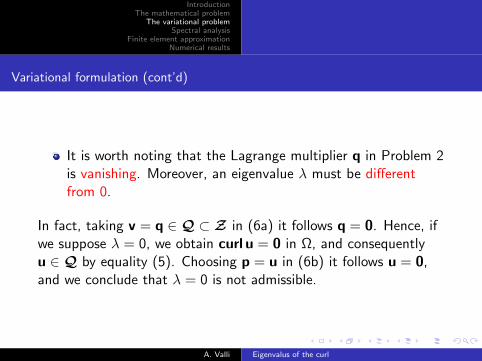
Figure: Test 3. Left to right. Eigenfunctions corresponding to theeigenvalues λh,1 = 8.815 and λh,2 = 8.912 for the case g = 2, g1 = 0(mesh with Nh = 10240).





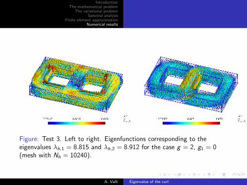
Figure: Test 3. Left to right. Eigenfunctions corresponding to theeigenvalues λh,3 = 10.561 and λh,4 = 10.611 for the case g = 2, g1 = 0(mesh with Nh = 10240).





Figure: Test 3. Eigenfunction corresponding to the eigenvalueλh,1 = 8.874 for the case g = 2, g1 = 1 (mesh with Nh = 10240).





References

J. Cantarella, D. DeTurck, H. Gluck and M. Teytel,Isoperimetric problems for the helicity of vector fields and theBiot–Savart and curl operators, J. Math. Phys., 41 (2000:a),5615–5641.

J. Cantarella, D. DeTurck and H. Gluck, The spectrum of thecurl operator on spherically symmetric domains, Phys.Plasmas, 7 (2000:b), 2766–2775.

R. Hiptmair, P.R. Kotiuga and S. Tordeux, Self-adjoint curloperators, Ann. Mat. Pura Appl. (4), 191 (2012), 431–457.

A.D. Jette, Force-free magnetic fields in resistivemagnetohydrostatics, J. Math. Anal. Appl., 29 (1970),109–122.





References (cont’d)

R. Kress, Ein Neumannsches Randwertproblem bei kraftfreinenFeldern, Meth. Verf. Math. Phys., 7 (1972), 81–97.

R. Kress, On constant-alpha force-free fields in a torus, J.Engrg. Math., 20 (1986), 323–344.

E. Lara, R. Rodrıguez and P. Venegas, Spectral approximationof the curl operator in multiply connected domains, DiscreteContin. Dyn. Syst. Ser. S, 9 (2016), 235–253.

E.C. Morse, Eigenfunctions of the curl in annular cylindricaland rectangular geometry, J. Math. Phys., 48 (2007), pp. 11,083504.

R. Picard, Ein Randwertproblem in der Theorie kraftfreierMagnetfelder, Z. Angew. Math. Phys., 27 (1976), 169–180.





References (cont’d)

R. Picard, On a selfadjoint realization of curl and some of itsapplications, Ricerche Mat., 47 (1998), 153–180.

R. Rodrıguez and P. Venegas, Numerical approximation of thespectrum of the curl operator, Math. Comp., 83 (2014),553–577.

L. Woltjer, A theorem on force-free magnetic fields, Proc.Nat. Acad. Sci. U.S.A., 44 (1958), 489–491.

Z. Yoshida and Y. Giga, Remarks on spectra of operator rot,Math. Z., 204 (1990), 235–245.





Proof. We define the following operator:

R : Vh −→ H(curl; Ω) ,vh 7−→ Rvh = vh −Φvh ,

with Φvh ∈Q is such that∫Ω

Φvh · p =

∫Ω

vh · p ∀p ∈Q .

From the inclusions Q ⊂ Z and Zh ⊂ Z we have at onceRvh ∈ Z, and from the definition of Φvh it follows Rvh⊥Q.





Consequently, Rvh ∈ V ⊂ H(curl; Ω) ∩ H0(div 0; Ω) ⊂ Hs(Ω)3 fors > 1/2. In addition, curl(Rvh) = curl vh ∈ curl(N k

h ). Hence wehave that INh (Rvh) is well-defined, and

‖Rvh − INh (Rvh)‖0,Ω ≤ C hs‖Rvh‖s,Ω + h‖curl(Rvh)‖0,Ω .(11)

Since Rvh ∈ V we obtain

‖Rvh‖s,Ω ≤ C‖Rvh‖Y ≤ C‖curl(Rvh)‖0,Ω. (12)

Employing the previous result and (11), we have

‖Rvh − INh (Rvh)‖0,Ω ≤ C (hs + h)‖curl(Rvh)‖0,Ω. (13)





The Nedelec interpolant INh Φvh is defined byINh Φvh = INh vh − INh (Rvh) = vh − INh (Rvh) and, sincecurl INh (Rvh) = curl vh, it follows that curl(INh Φvh) = 0 in Ω.Furthermore,

∮γ′j

INh Φvh · t′j =∮γ′j

Φvh · t′j = 0 for j = g1 + 1, . . . , g ,

as Φvh ∈Q. In conclusion, INh Φvh ∈Qh.Employing this result and the fact that INh vh = vh, we obtain

‖vh‖20,Ω =

∫Ω

vh · INh vh =

∫Ω

vh ·(

INh (Rvh) + INh Φvh

)=

∫Ω

vh · INh (Rvh) ,

as vh ∈ Vh. Using inequalities (13) and (12), and the fact thatcurl(Rvh) = curl vh in Ω, we obtain





‖vh‖0,Ω ≤ ‖INh (Rvh)‖0,Ω ≤ ‖Rvh − INh (Rvh)‖0,Ω + ‖Rvh‖0,Ω

≤ C (hs + h)‖curl vh‖0,Ω + C‖curl vh‖0,Ω

≤ C‖curl vh‖0,Ω,

which concludes the proof. 2





Proof. First note that, by proceeding as in the proof ofLemma 11, we have that, for all f ∈ E,

‖(T− Th)f‖curl;Ω ≤ Chminr ,k (‖Tf‖r ,Ω + ‖curl Tf‖r ,Ω)

≤ Chminr ,k supg∈E

‖Tg‖r ,Ω + ‖curl Tg‖r ,Ω‖g‖curl;Ω

‖f‖curl;Ω

≤ C ′hminr ,k‖f‖curl;Ω ,(14)

where we have used the fact that E is finite dimensional for thelast inequality. Therefore (9) follows from (14) and Babuska andOsborn [Chap. II, Theor. 7.1].





To prove (10), let f, g ∈ E ⊂ V be two eigenfunctions. Then, inparticular, g satisfies

curl g = λg in Ω . (15)

If we define u := Tf and uh := Thf, then the following identitiesare satisfied∫

Ωcurl u · curl v =

∫Ω

f · curl v ∀v ∈ Z∫Ω

curl uh · curl vh =

∫Ω

f · curl vh ∀vh ∈ Zh .

Subtracting both identities, we obtain∫Ω

curl(u− uh) · curl vh = 0 ∀vh ∈ Zh. (16)





In addition, let w := Tg and wh := Thg. Then we have analogousidentities for g and, in particular,∫

Ωcurl w · curl v =

∫Ω

g · curl v ∀v ∈ Z. (17)

Thus, thanks to (15), the fact that u, uh, g ∈ Z, Lemma 6, (16)and (17), we obtain∫

Ω(T− Th)f · g = λ−1∫

Ω(u− uh) · curl g

= λ−1∫

Ω curl(u− uh) · g

= λ−1∫

Ω curl(u− uh) · curl(w −wh)

= λ−1∫

Ω curl((T− Th)f) · curl((T− Th)g) .





Using Cauchy–Schwarz inequality and (14) we get∣∣∫Ω(T− Th)f · g

∣∣ ≤ λ−1‖(T− Th)f‖curl;Ω‖(T− Th)g‖curl;Ω

≤ Cλ−1h2 minr ,k‖f‖curl;Ω‖g‖curl;Ω.(18)

On the other hand, thanks to (16), Cauchy–Schwarz inequality,(14), Lemma 5 and Monk [Theorem 5.41], we obtain∣∣∫

Ω curl(T− Th)f · curl g∣∣ =

∣∣∫Ω curl(u− uh) · curl g

∣∣=∣∣∣∫Ω curl(u− uh) · curl(g − INh g)

∣∣∣≤ Chminr ,k ‖f‖curl;Ω hminr ,k(‖g‖r ;Ω + ‖curl g‖r ,Ω)

≤ C ′h2 minr ,k ‖f‖curl;Ω ‖g‖curl;Ω .(19)





Thus, from (18) and (19) we conclude that

supf,g∈E

∣∣∫Ω(T− Th)f · g +

∫Ω curl(T− Th)f · curl g

∣∣‖f‖curl;Ω‖g‖curl;Ω

≤ Ch2 minr ,k .

Estimate (10) follows from Babuska and Osborn [Chap. II, Theor.7.3] and the fact that T is self adjoint. 2


Eigenvalues of the curl operator: variational formulation and ...

Documents

Transcript of Eigenvalues of the curl operator: variational formulation and ...