A simultaneous successive linear estimator and a guide for

hydraulic tomography analysis

Jianwei Xiang,1 Tian-Chyi J. Yeh,1,2 Cheng-Haw Lee,2 Kuo-Chin Hsu,2

and Jet-Chau Wen3

Received 22 May 2008; revised 8 December 2008; accepted 23 December 2008; published 28 February 2009.

[1] In this study, a geostatistically based estimator is developed that simultaneouslyincludes all observed transient hydrographs from hydraulic tomography to mapaquifer heterogeneity. To analyze tomography data, a data preprocessing procedure(including diagnosing and wavelet denoising analysis) is recommended. A least squaresapproach is then introduced to estimate effective parameters and spatial statistics ofheterogeneity that are the required inputs for the geostatistical estimator. Since waveletdenoising does not completely remove noise from observed hydrographs, a stoppingcriterion is established to avoid overexploitation of the imperfect hydrographs. Theestimator and the procedures are then tested in a synthetic, cross-sectional aquifer withhierarchical heterogeneity and a vertical sandbox with prearranged heterogeneity. Resultsof the test indicate that with this estimator and preprocessing procedures, hydraulictomography can effectively map hierarchical heterogeneity in the synthetic aquifer as wellas in the sandbox. In addition, the study shows that using the estimated hydraulicconductivity and specific storage fields of the sandbox, the classic groundwater flowmodel accurately predicts temporal and spatial distributions of drawdown induced by anindependent pumping event in the sandbox. On the other hand, the classic groundwaterflow model yields less satisfactory results when equivalent homogeneous properties ofthe sandbox are used.

Citation: Xiang, J., T.-C. J. Yeh, C.-H. Lee, K.-C. Hsu, and J.-C. Wen (2009), A simultaneous successive linear estimator and a guide

for hydraulic tomography analysis, Water Resour. Res., 45, W02432, doi:10.1029/2008WR007180.

1. Introduction

[2] Classical aquifer test which involves one pumpingwell and an observation well has been shown to yieldambiguously averaged hydraulic properties of an aquifer,which vary with the location of observation and pumpingwells, and heterogeneity [Wu et al., 2005; Liu et al., 2007;Straface et al., 2007; Kuhlman et al., 2008]. To avoidobtaining the ambiguously averaged estimates and to providehigh-resolution aquifer characterization, a new aquifer char-acterization technology, known as hydraulic tomography(HT), has recently been developed [e.g., Tosaka et al., 1993;Gottlieb and Dietrich, 1995; Vasco et al., 2000; Yeh andLiu, 2000; Bohling et al., 2002; Brauchler et al., 2003; Zhuand Yeh 2005, 2006]. Although the ability of HT remainsto be fully assessed under field conditions, results fromsandbox experiments by Liu et al. [2002], Illman et al.[2007, 2008], and Liu et al. [2007] are encouraging.These studies showed that the transient HT can identify

not only the pattern of the heterogeneous hydraulic con-ductivity (K) field, but also the variation of specificstorage (Ss) in the sandbox. Moreover, these estimatedK and Ss fields from the HT sandbox experiments furtherpredicted the drawdown evolution caused by a pumpingtest that was not used in the HT analysis. Likewise, arecent application of HT to a well field at MontaltoUffugo Scalo, Italy, produced an estimated transmissivityfield that is deemed to be consistent with the geology ofthe site [Straface et al., 2007]. Bohling et al. [2007] andLi et al. [2007] also showed promising results of HT intheir field experiments.[3] Most of HT analyses in the past have used the

sequential successive linear estimator (SSLE) of Yeh andLiu [2000] or Zhu and Yeh [2005], which includes data setsfrom HT surveys sequentially. Illman et al. [2008] reportedthat the order of test data included in SSLE affected the finalestimates. In addition, little efforts in the past have focusedon investigation of effects of noise in well hydrographson the analysis of HT and development of methods forremoving the noise. In this paper, we thereby develop ageostatistically based method for identifying the subsurfaceheterogeneity pattern using all the data collected from aHT survey simultaneously, similar to the approaches byVesselinov et al. [2001], Li et al. [2007], Fienen et al.[2008], or Li et al. [2008], which are built upon the quasi-linear geostatistical approach [Kitanidis, 1995]. Moreover, acriterion for the nonlinear estimator is developed to deter-

1Department of Hydrology and Water Resources, University of Arizona,Tucson, Arizona, USA.

2Department of Resources Engineering, National Cheng Kung University,Tainan, Taiwan.

3Department of Environmental and Safety Engineering, Research Centerfor Soil and Water Resources and Natural Disaster Prevention, NationalYunlin University of Science and Technology, Touliu, Taiwan.

Copyright 2009 by the American Geophysical Union.0043-1397/09/2008WR007180$09.00

W02432

WATER RESOURCES RESEARCH, VOL. 45, W02432, doi:10.1029/2008WR007180, 2009ClickHere

for

FullArticle

1 of 14

mine the appropriate level of improvement of estimationwhen hydrographs are infested with noise. We also proposea procedure for preprocessing HT data before application ofthe estimator. This estimator and procedure were tested in asynthetic aquifer with hierarchical heterogeneity [Barrashand Clemo, 2002; Ye et al., 2005], and then applied to asandbox experiment, which involves unknown measure-ment errors and where our mathematical model may notcorrectly describe the flow process model errors.

2. Methodology

2.1. Governing Groundwater Flow Equations

[4] A strategy for modeling groundwater flow in saturated,heterogeneous, porous media with incomplete specificationof aquifer characteristics is the stochastic conditional meanapproach [e.g., Yeh et al., 1996]. That is, the flow processis governed by the following partial differential equationinvolving conditional means:

r � K xð Þrh½ � þ Q xp� �

¼ Ss xð Þ @h@t

; ð1Þ

subject to boundary and initial conditions:

h G1j ¼ h1; K xð Þrh½ � � n G2

j ¼ q; and h t¼0 ¼ h0j ; ð2Þ

where, in equation (1), h is conditional effective total head(L), x is the spatial coordinate (x = {x, y}, (L), and yrepresents the vertical coordinate and is positive upward) inthe two-dimensional, cross-sectional aquifers examined inthis paper, Q(xp) is the pumping rate (1/T) at the location xp,K(x) is the conditional effective saturated hydraulic con-ductivity (L/T), and Ss(x) is the conditional effective spe-cific storage (1/L). In equation (2), h1 is the prescribed totalhead at Dirichlet boundary G1, q is the specific discharge(L/T) at Neumann boundary G2, n is a unit vector normalto G2, and h0 represents the initial total head. The definitionsof variables in the conditional mean equations are identicalto those in a deterministic groundwater flow equation if allthe parameters, boundary and initial conditions are fullyspecified [Yeh et al., 1996]. In this paper, these governingequations are used to simulate the flow field during theHT survey and are solved by a 2-D finite element model(VSAFT2) developed by Yeh et al. [1993].

2.2. Simultaneous Successive Linear Estimator

[5] Instead of incorporating data sequentially into theestimation as is done in SSLE, a simultaneous successivelinear stochastic estimator (SimSLE) is developed to includeall drawdown data from different pumping tests during a HTsurvey simultaneously to estimate hydraulic properties ofaquifers. Simultaneous inclusion of the data offers someadvantages over the SSLE approach (see discussion section).Below is a brief description of the SimSLE.[6] With given unconditional mean and spatial covariance

functions of the hydraulic properties (prior joint probabilitydistribution, implicitly Gaussian), the SimSLE starts withcokriging (a stochastic linear estimator) to estimate theconditional expected value of the property conditioned onf *(xi) (i.e., perturbations of log hydraulic property, K and/or

Ss) measured at ith location (i = 1, . . . Nf, where Nf is thetotal number of f measurements) and the observed head atlocation xj at time t‘ during kth pumping test, denoted byh*(k, xj, t‘). The linear estimator is

f 1ð Þ x0ð Þ ¼XNf

i¼1

l0i f * xið Þ þXNp

k¼1

XNh kð Þ

j¼1

XNt k;jð Þ

‘¼1

� m0k j ‘ h* k; xj; t‘� �

he k; xj; t‘� �� �

; ð3Þ

where f (1)(x0) is the cokriged f value at location x0; he(k, xj,t‘) is the simulated head at the observation location and timeof the pumping test, based on effective properties of anequivalent homogeneous medium; Np is the total number ofpumping tests; Nh(k) is the total number of observationlocations for kth pumping test; Nt (k, j) is the total number ofhead measurements in time at jth observation locationduring kth pumping test. The cokriging weight (l0i) repre-sents contribution of measurement f * at ith location to theestimate at location x0. The contribution to the estimatefrom the observed head h*(k, xj, t‘) is denoted by m0kj‘.These weights are obtained by solving the following systemof equations:

XNf

i¼1

l0iRff xm; xið Þ þXNp

k¼1

XNh kð Þ

j¼1

XNt k;jð Þ

‘¼1

� m0kj‘Rhf k; xj; t‘� �

; xm� �

¼ Rff x0; xmð ÞXNf

i¼1

l0iRhf p; xr; tq� �

; xi� �

þXNp

k¼1

XNh kð Þ

j¼1

XNt k;jð Þ

‘¼1

� m0kj‘Rhh p; xr; tq� �

; k; xj; t‘� �� �

¼ Rhf p; xr; tq� �

; x0� �

; ð4Þ

in whichm = 1, . . . Nf, p = 1, . . . Np, r = 1, . . . Nh(p) and ‘ andq = 1, . . .Nt(p, r). Our prior knowledge of the spatial structure(the unconditional covariance function) of f is given by Rff.Rhh and Rhf are the unconditional covariance of h andthe unconditional cross covariance of f and h, respectively,which are determined by a first-order analysis with the givenRff. That is,

Rhf k; xi; t‘ð Þ; xmð Þ ¼XNe

j¼1

J k; xi; t‘ð Þ; xj� �

Rff xj; xm� �

k ¼ 1; . . .Np; i ¼ 1; . . .Nh kð Þ; ‘ ¼ 1; . . .Nt k; ið Þ; m ¼ 1; . . .Ne

ð5Þ

Rhh u; xi; tq� �

; k; xj;t‘� �� �

¼XNe

m¼1

Rhf u; xi; tq� �

; xm� �

J ðk; xj;t‘�;xm

� �Tu and k ¼ 1; . . .Np; i and j ¼ 1; . . .Nh u or kð Þ;q and ‘ ¼ 1; . . .Nt u or k; ið Þ; ð6Þ

where J((k, xj, t‘), xm) is the sensitivity of head at jthlocation at time t‘ for kth pumping test with respect to thechange of parameter at mth location; Ne is the number ofelements in the study domain. The sensitivity matrix isevaluated using an adjoint state approach (see Zhu and Yeh[2005] for details).

ð4Þ

ð5Þ

ð6Þ

2 of 14

W02432 XIANG ET AL.: SIMULTANEOUS SUCCESSIVE LINEAR ESTIMATOR W02432

[7] After obtaining the new estimate for all the elementsusing cokriging, the conditional covariance of f, eff

(1)(xm, xq),is then determined by

e 1ð Þff xm; xq� �

¼ Rff xm; xq� �

XNf

k¼1

lmkRff xk ; xq� �

XNp

k¼1

XNh kð Þ

j¼1

XNt k;jð Þ

‘¼1

mmkj‘Rhf k; xj; t‘� �

; xq� �

; ð7Þ

where m and q = 1, . . . Ne. The conditional covariancereflects the effect of data on the reduction of uncertainty inthe estimated parameter field. Subsequently, the estimatedlog perturbations of the property fields are added to the logof the effective properties, F(x), then converted to thearithmetic scale, and used to solve equation (1) withboundary and initial conditions for the conditional effectivehead fields, h(1)(k, xj, t‘), of each pumping test.[8] Following cokriging, a linear estimator of the follow-

ing form,

f rþ1ð Þ x0ð Þ ¼ f rð Þ x0ð Þ þXNp

k¼1

XNh kð Þ

j¼1

XNt k;jð Þ

‘¼1

� w rð Þ0kj‘ h* k; xj; t‘

� � h rð Þ k; xj; t‘

� �h i; ð8Þ

is used to improve the estimate for iteration r > 1, wherew0kj‘(r) is the weight term, representing the contribution of the

difference between the observed and simulated conditionalheads (i.e., h*(k, xj, t‘) and h(r)(k, xj, t‘), respectively) atiteration r at location xj of the kth pumping test at time t‘ tothe estimate at location x0. The weights are determined bysolving the following system of equations:

XNp

k¼1

XNh kð Þ

j¼1

XNt k;jð Þ

‘¼1

w rð Þ0kj‘ e rð Þ

hh p; xm; tq� �

; k; xj; t‘� �� �h

þ Q rð Þdkj‘i

¼ e rð Þhf p; xm; tq

� �; x0

� �; ð9Þ

where p = 1, . . . Np, m = 1, . . . Nh(p) and q = 1, . . . Nt(p, m).The terms ehh

(r) and efh(r) are the conditional covariance and the

conditional cross covariance at iteration (r), which areevaluated using equations (5) and (6) using the conditionalcovariance of f (i.e., eff

(r) which is obtained from equation (7)for the first iteration). A dynamic stabilizer, Q(r), is added tothe diagonal elements of ehh

(r) (dkjl is a Dirac delta, equal to 1when k = j = l and zero otherwise) to stabilize the solution toequation (9). The dynamic stabilizer at iteration, r, is themaximum value of the diagonal elements of ehh

(r) at thatiteration times a user-specified multiplier [see Yeh et al.,1996]. After completion of the estimation using equation (8)for all elements in the domain, the conditional covariance off is updated subsequently as given below:

e rþ1ð Þff xm; xnð Þ ¼ e rð Þ

ff xm; xnð Þ

XNp

k¼1

XNh kð Þ

j¼1

XNt k;jð Þ

‘¼1

wmkj‘erð Þhf k; xj; t‘

� �; xn

� �; ð10Þ

where n and m = 1, . . . Ne.

[9] The iteration steps of SimSLE are the same as those inthe SLE algorithm used by Yeh et al. [1996]. For noise-freehydrographs, the convergence is achieved if (1) change invariances that represent spatial variability of the estimatedhydraulic properties between current and last iterations issmaller than a specified tolerance (i.e., the spatial varianceof the estimates stabilizes), implying that the SimSLE cannotimprove the estimation any further and (2) change of simu-lated heads between successive iterations is smaller than thetolerance, indicating that the estimates will not significantlyimprove the head field. If one of the two criteria is met, theestimates are considered to be optimal and the iterations areterminated.[10] Head observations from laboratory or field experi-

ments often contain noise (i.e., signals caused by processesnot modeled by the governing flow equation, such as Earthtide and others including measurement errors) in addition toeffects of hierarchical heterogeneity. Such unresolved noisescan lead to divergence of inverse solutions (i.e., unrealisticestimates). As a consequence, an important issue that oughtto be addressed is to what degree should the observed headbe used to improve estimates of the hydraulic properties.Stabilization of mean square error of the simulated headduring iteration should address the issue. Consider the meansquare error of the head:

E h* k; x; tð Þ h rð Þ k; x; tð Þ� �2

� ¼ E h k; x; tð Þ þ tð Þ h rð Þ k; x; tð Þ

� �2�

¼ E h k; x; tð Þ h rð Þ k; x; tð Þ� �2

� þE t2

�¼ e rð Þ

hh k; x; tð Þ þ s2t ; ð11Þ

in which the observed head at location x and time t duringkth pumping event is denoted by h*(k, x, t); the cor-responding simulated head based on the estimated para-meters at rth iteration is given by h(r)(k, x, t). Equation (11)assumes that the observed head consists of the noise freehead, h(k, x, t), and random noise, t, with variance st

2. Theterm ehh

(r)(k, x, t) denotes the theoretical residual headvariance for the noise free case at rth iteration (i.e., thediagonal term in equation (6)), which should decrease andapproach zero with iterations because of improvement ofthe parameter estimates. Therefore, the mean square errorfor cases with noise should asymptotically converge to st

2

as the number of iterations increases. More importantly,equation (11) suggests that once ehh

(r)(k, x, t) becomes smallerthan st

2 (i.e., the mean square error stabilizes), the iterationshould stop to avoid overusage of imperfect head data (i.e.,updating the estimate with noise). Consequently, for caseswhere the observed head is not noise free, we use thestabilization of the L2 norm of the conditional heads toterminate the iteration, i.e.,

L2cond rð Þ ¼ 1

N

XNi¼1

hi* hrð Þi

� �2

; ð12Þ

where h*i and hi(r) are observed and simulated heads,

respectively; i is the index denoting the observation in agiven time and location from a pumping test; N is the totalnumber of head observations from all the pumping tests.

W02432 XIANG ET AL.: SIMULTANEOUS SUCCESSIVE LINEAR ESTIMATOR

3 of 14

W02432

Hereafter, we will refer to equation (12) as to the conditionalL2 norm.

2.3. Preprocessing Data for SimSLE

2.3.1. Diagnosis of Bias[11] The first step in preprocessing HT data for the

SimSLE analysis is to qualitatively check for any bias orinconsistency in the data. We suggest this be accomplishedby a simple rule-of-thumb approach: plotting hydrographs(drawdown time data) for each pumping test. For example,arrival time of a given drawdown should increase withdistance from the pumping well unless there are physicallyexplainable anomalies (e.g., fracture zones or other fast flowpaths). Plots of evolution of contour surface of the draw-down induced by each pumping test generally should followbehaviors of drawdown in homogeneous aquifers [e.g.,Bakr et al., 1978] although details are different. Data withsignificant anomalies should be examined for possibleoperational causes (e.g., mislabeling monitoring ports orwells, leakage between packers, malfunctioning of equip-ment, or other factors). If the operational causes can beidentified, the data sets should be corrected or excluded.Repeating the HT experiment also facilitates a viablediagnosis. Drawdown-log time plots should also revealpossible boundary effects and they are useful in assigningthe type of boundary conditions of the modeling domain.2.3.2. Wavelet Denoising[12] Next, we tackle data noise or signals or perturbations

caused by factors other than aquifer heterogeneity. Toeliminate the noise, a denoising method based on waveletanalysis [e.g., Mallat, 1999; Zhang et al., 2006] wasdeveloped. A wavelet analysis is similar to Fourier analysisin the sense that it breaks a signal down into its constituentparts for analysis. In contrast to the Fourier transform, thewavelet transform allows exceptional localization in boththe time domain via translations of the mother wavelet, andthe scale (frequency) domain via dilations, when analyzingsignals of a nonstationary nature. Software from http://www.mathworks.com was used. Different families of

wavelets were tested in this study and we found that theDaubechies 4 wavelet is effective for our cases.[13] The wavelet denoising procedure used in this study

comprises the following steps: (1) applying the wavelettransform to the noisy hydrograph to produce waveletcoefficients, (2) selecting an appropriate threshold limitand a threshold method to remove the noise, (3) inversingthe wavelet transform of thresholded wavelet coefficients togenerate a denoised hydrograph, and (4) calculating thevariance of the difference between the denoised hydrographsand those of the equivalent homogenous medium. Thisvariance should be approximately equal to the theoreticalhead variance from the first-order analysis. If this criterionis not met, repeat steps 2 and 3. Generally speaking,distinguishing noise from the effects of heterogeneity in ahydrograph can be highly subjective unless characteristicsof noise or heterogeneity are known a priori.

2.4. Signal-to-Noise Ratio

[14] Following wavelet denoising, we examined the signal-to-noise ratio (SNR) of each well hydrograph. The SNR is anelectrical engineering concept, which is defined as the ratio ofsignal amplitude to noise amplitude. In our study, it is definedas the ratio between the maximum drawdown of the denoisedhydrograph and the standard deviation of noise. That is,

SNR ¼ signal

noise¼ hd x; 0ð Þ hd x; tð Þj jð Þmax

Sn

; ð13Þ

where j j denotes the absolute value; hd denotes the headafter denoising; and Sn represents the standard deviationof noise, which is estimated from the wavelet denoisingprocedure. In signal processing, signals with SNR of 100 orgreater are considered to be good signals. For hydrologicprocesses, we found that hydrographs with an average SNR of7.13 or greater are effective for our synthetic case. Figure 1ashows an original hydrograph from Illman et al. [2007,2008] and Liu et al. [2007] and the corresponding denoisedhydrograph; the SNR is 17.75. The denoised hydrograph

Figure 1. Typical hydrographs and corresponding denoised hydrographs (solid black line) in thesandbox experiments [Liu et al., 2007]: (a) SNR 17.75 and (b) SNR 4.41. Notice vertical exaggeration.

4 of 14

W02432 XIANG ET AL.: SIMULTANEOUS SUCCESSIVE LINEAR ESTIMATOR W02432

therefore is considered useful and it improves the estimates.On the other hand, a hydrograph with low-SNR data (4.41)(Figure 1b), especially near the falling and rising limbs ofthe graph (reflecting effects of pumping and recovery,respectively), was discarded since it did not improve theestimates. Low-SNR data at early time and recovery canlead to erroneous estimates of the Ss field. As a rule ofthumb, the SNR should be much greater than 1 such that thetrend of drawdown induced by pumping is evident afterdenoising. However, a more in-depth analysis is needed toestablish a rigorous criterion.

2.5. Estimation of Effective Properties and Variances

[15] Afterward, desirable hydrographs from the HT wereselected to estimate unconditional effective K and Ss of anequivalent homogeneous medium with the known pumpingrates. This task was accomplished by minimizing thesquared difference between the observed head values andthose obtained from simulations based on the homogeneityassumption using the VSAFT2:

Xnpi¼1

Xnhj¼1

Xntk¼1

hijk* Hijk

� �2¼ min

K;Ss: ð14Þ

In the above equation, h*ijk denotes observed head at kthtime, jth observation location, and ith pumping test, and thecorresponding simulated head using the unconditionaleffective K and Ss is indicated by H ijk. Minimization ofequation (14) was performed using a standard nonlinearleast squares (i.e., Gauss-Newton) approach in conjunctionwith the Levenberg-Marquardt algorithm [Press et al.,1992]. Sensitivity matrices were evaluated by solving thesensitivity equation (i.e., differentiation of equation (1) withrespect to the parameter).[16] Subsequently, square of the difference between the head

observed and the head in the equivalent homogeneousmediumis used to compute the sample variance of the observed headat the given location and time. This sample head varianceis in turn used to estimate the variance of the hydraulicproperties by minimizing the following objective function:

Xnpi¼1

Xnhj¼1

Xntk¼1

s2ijk s2

ijk

� �2

¼ minimum; ð15Þ

where sijk2 is the sample head variance and sijk

2 is the theo-retical head variance at kth time, jth observation location, andith pumping test. This theoretical head variance is evaluatedusing the first-order approximation (i.e., equation (6)) withgiven variance of the hydraulic properties. The Levenberg-Marquardt algorithm was used to seek the variances of theproperties that minimize equation (15). Relative change ofequation (15) between successive iterations is used as con-vergence criterion. These estimated effective hydraulic prop-erties and variances are used as prior information required bySimSLE for estimating the spatially varying K and Ss fields.

3. Applications to a Synthetic Aquifer

3.1. Description of the Aquifer and HT Test

[17] To test our SimSLE and the data preprocessingprocedure for the HT analysis, a two-dimensional, cross-

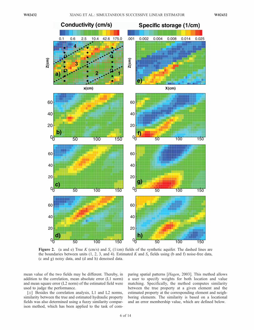
sectional, synthetic aquifer of the same length and height asthe sandbox experiment conducted by Illman et al. [2007,2008] and Liu et al. [2007] was used. The dimensions of thesandbox were 193.0 cm in length, 82.6 cm in height, and10.2 cm in depth. Twenty four locations were selected (solidcircles in Figure 2a) to serve as pressure monitoring portsduring four pumping tests at four locations (open circles inFigure 2a). Both sides of the aquifer were set to the sameconstant boundary condition with a total head of 200 cm,while the bottom and top boundaries were set to be no-fluxboundaries. The initial total head was assigned to be 200 cm.This aquifer was discretized into 741 elements and 800 nodeswith element dimensions of 4.10 cm � 4.13 cm.[18] The synthetic aquifer was created to imitate a geologic

formation of hierarchical heterogeneity, consisting of fourunits with a bedding dip angle of 20�. The ln K and ln Ssfields within each unit were assumed to be normally distrib-uted random fields with different means and variances (seeTable 1). An exponential model was used as the spatialcovariance functions of the fields with correlation scales of200 cm in the bedding direction and 12 cm in the directionperpendicular to bedding. Different random seed numberswere used to create the ln K and ln Ss fields (Figures 2a and 2e,respectively) so that they are independent of each other.[19] Four pumping tests in this aquifer were simulated

using a time step of 0.25 s for a period of 15 s at which thedrawdown reached a steady state condition because of thesmall size of the aquifer. Each pumping test had a pumpingrate of 0.3 cm3/s and drawdown at all 24 wells wererecorded. These simulated drawdown-time data sets wereregarded as noise-free hydrographs. These noise-free hydro-graphs were subsequently corrupted by adding normallydistributed white noise with a standard deviation of 0.07 cmto represent measurement errors and these corrupted hydro-graphs are denoted as noisy hydrographs. Finally, thewavelet denoising procedure was applied to these noisyhydrographs to obtain the so-called denoised hydrographs.The SNR values of the 96 corrupted hydrographs were foundmuch greater than 1 and all the hydrographs were includedin the following HT analysis.[20] To investigate the ability of SimSLE to estimate the

heterogeneous K and Ss fields, drawdowns at 5 times (fourearly times at 0.5 s, 1.75 s, 2.25 s and 3 s; and one later timeat 15 s) from the noise-free, noisy, and denoised HThydrographs were used. Such a choice of sampling timesstems from the finding by Wu et al. [2005] that thedrawdown at early time is highly correlated with the Ssfield and only weakly and negatively correlated with the Kfield in the area between the pumping and the observationlocations. At large time, the drawdown is correlated at variousdegrees with K values in the area within the cone ofdepression but not the Ss field. In the estimation, K and Ssvalues at the top observation port in the left column inFigure 2a were assumed to be known and they were used asthe hard data for conditioning the estimation in all the cases.

3.2. Performance Assessment

[21] Performance of our estimator for the synthetic aquifercase was evaluated using the standard correlation coefficient(1 � jrj � 0) which measures the similarity between the trueand the estimated fields. A correlation coefficient close to 1means the two fields are similar in pattern, even though the

W02432 XIANG ET AL.: SIMULTANEOUS SUCCESSIVE LINEAR ESTIMATOR

5 of 14

W02432

mean value of the two fields may be different. Thereby, inaddition to the correlation, mean absolute error (L1 norm)and mean square error (L2 norm) of the estimated field wereused to judge the performance.[22] Besides the correlation analysis, L1 and L2 norms,

similarity between the true and estimated hydraulic propertyfields was also determined using a fuzzy similarity compar-ison method, which has been applied to the task of com-

paring spatial patterns [Hagen, 2003]. This method allowsa user to specify weights for both location and valuematching. Specifically, the method computes similaritybetween the true property at a given element and theestimated property at the corresponding element and neigh-boring elements. The similarity is based on a locationaland an error membership value, which are defined below.

Figure 2. (a and e) True K (cm/s) and Ss (1/cm) fields of the synthetic aquifer. The dashed lines arethe boundaries between units (1, 2, 3, and 4). Estimated K and Ss fields using (b and f) noise-free data,(c and g) noisy data, and (d and h) denoised data.

6 of 14

W02432 XIANG ET AL.: SIMULTANEOUS SUCCESSIVE LINEAR ESTIMATOR W02432

[23] An exponential function based on the statisticalspatial model for the hydraulic properties was used to definea locational membership

Vl ¼ exp

ffiffiffiffiffiffiffiffiffiffiffiffiffiffiffiffiffiffiffiffiffiffiffiffiffiffiffiffiffiffiffilx

lx

�2

þ ly

ly

�2s0

@1A: ð16Þ

In which lx and ly are the separation distance between twocompared elements in the x and y directions; lx and ly arethe correlation scale of the true property field in the x and ydirections, respectively. Equation (16) implies that thesimilarity decreases with an increase of the ratio of theseparation distance to the correlation scale.[24] The standard deviation of the true property (STD) is

used as an error limit and to define the value of the errormembership:

Vv ¼1:0 vj j

STD

vj jSTD

< 1

0vj j

STD� 1;

8>><>>: ð17Þ

where v is the difference between the true property at a givenelement and the estimated property at a selected element.That is, if the difference of two properties is greater than thestandard deviation, the two properties are judged to becompletely different. Otherwise, a linear decay is used todetermine the error membership value.[25] The true property of an element in the domain is then

compared with the estimated property of the same elementand with the estimated property of neighboring elements(within the correlation scales). Equations (16) and (17) areemployed to determine the locational and error membershipvalues. For each pair of the true and the estimated property,a similarity value is then computed by multiplying thelocational membership with the error membership. Onlythe maximum value among the similarity values of all pairsis retained for the selected element. Next, the maximumsimilarity between the estimated property at that element

with the true property at the corresponding element andat neighboring elements is determined. The similarity valuebetween the true and the estimated properties of thiselement is then defined by the average of the two maximumsimilarities. This procedure is applied to all the elements inthe synthetic domain. Finally, a domain similarity is definedas the average element similarity of all elements in thedomain.

3.3. Results

[26] Table 2 tabulates the estimated effective K and Ssvalues for an equivalent homogeneous and isotropic porousmedium of the synthetic aquifer, using the noise-free, noisy,and denoised hydrographs. Estimated variances of ln K andln Ss over the entire aquifer are also listed in Table 2, whichwere obtained using equation (15) with visually estimatedcorrelation scales (100 cm and 33 cm, in the direction paralleland perpendicular to bedding, respectively) and the knowndip angle. Table 2 shows that the estimated effective proper-ties based on the noise-free, noisy, and denoised hydrographsare similar. Estimated effective K values are found to beslightly greater than the geometric mean while the effectiveSs values are in agreement with the arithmetic mean of thecorresponding values of the four units. Apparently, noisedoes not have significant effects on the estimates of theeffective properties since this is an overdetermined inverseproblem (i.e., more data than parameters need to be esti-mated and the problem is well posed [Yeh et al., 2007]. Theleast squares approach is expected to be sufficient andeffective.[27] As shown in Table 2, estimated variances of ln K and

ln Ss with equation (15) are smaller than the true ones, likelydue to insufficient head data. The nonstationary nature ofthe drawdown (i.e., its variance depends on the spatially andtemporally varying mean gradient) demands a large numberof head data at the same radial distance from the pumpingwells to obtain a representative sample head variance inequation (15).[28] To illustrate the effectiveness of wavelet denoising,

480 pairs of observed heads before and after denoising atthe 24 ports at 5 sampling times during the 4 pumping testsand corresponding simulated heads based on effective K andSs are plotted as red circles in Figures 3a and 3b, respec-tively. Pluses in Figure 3 correspond to the simulated headsplus and minus one standard deviation of the theoreticalhead perturbation caused by heterogeneity, ehh

(0)(k, x, t). Acomparison of Figures 3a and 3b shows that the waveletdenoising removed most of perturbations of the total headsbetween 199.5 cm and 200 cm, which are not significantlyaffected by the pumping test. Head data after denoisingare generally within one standard deviation of the theoret-ical head perturbation caused by heterogeneity, suggesting

Table 2. Estimated Effective Hydraulic Properties and Estimated Spatial Variances of the Properties in the Synthetic

Aquifer Using Noise-Free, Noisy, and Denoised Hydrographsa

Cases Effective ln K (cm/s) Variance ln K Effective ln Ss (1/cm) Variance ln Ss Iterations

Synth (noise free) 1.422 0.679 5.114 0.442 16Synth noise 1.414 0.520 5.181 0.154 17Synth denoised 1.431 0.571 5.084 0.329 23

aThe number of iterations required to reach to the convergence of the solution is listed in the last column.

Table 1. Means and Variances of the Generated ln K and ln Ss

Field in Each Unit of the Synthetic Aquifer and Over the Entire

Aquifer

Unit 1 Unit 2 Unit 3 Unit 4 Overall

ln KMean 2.03 0.85 2.46 0.67 1.39Variance 1.01 0.17 2.00 0.46 2.18

ln SsMean 6.06 4.82 6.43 5.06 5.61Variance 0.05 0.24 0.01 0.08 0.66

W02432 XIANG ET AL.: SIMULTANEOUS SUCCESSIVE LINEAR ESTIMATOR

7 of 14

W02432

the remaining perturbations are likely effects of aquiferheterogeneity.[29] Table 3 lists values of unconditional L1 and L2

norms of the hydraulic head, which are defined as

L1un ¼1

N

XNi¼1

hi hi�� ��

L2un ¼1

N

XNi¼1

hi hi�� ��2;

where h is the simulated head in the equivalent homogeneousaquifer using the effective parameter values derived fromthe noise-free hydrographs; h is the noise-free, noisy, ordenoised heads of the heterogeneous aquifer, at the 5selected times during the four pumping tests (i.e., N = 480).These statistics aim to measure effects of the hierarchicalheterogeneity (i.e., spatial variability or structured noise),measurement noise, and noise residuals in hydrographs afterwavelet denoising. As expected, the noise-free hydrographhas the smallest unconditional L1 and L2 norms, reflectingthe effect of heterogeneity only. L1 and L2 norms are highestfor the noisy hydrographs where head perturbations areresults of both heterogeneity and the white noise. Values ofL1 and L2 norms in the last row of Table 3 for the denoisedhydrographs are between those of noise-free and noisyhydrographs, indicative of only partial removal of noise bythe wavelet denoising procedure. On the basis of the L2values, 92% of the perturbations in the noisy hydrographsare effects of hierarchical heterogeneity and the remaining8% are random noise. The wavelet denoising procedureremoved 80% of the random noise.

[30] Estimating 741 pairs of Ks and Ss of the syntheticaquifer on the basis of the 480 drawdowns and one pair ofKs and Ss hard data set is an underdetermined (i.e., over-parameterized or ill-posed [see Yeh et al., 2007]) inverseproblem. That is, the number of the parameters to beestimated is larger than the number of data sets available.While SLE aims to seek the estimate of the conditionaleffective parameters [Yeh et al., 1996] for underdeterminedproblems, the noise or unresolved noise may lead toanomalously high or low estimates. To circumvent thisproblem, the criterion based on the stabilization of theconditional L2 norm of the head (i.e., equation (12)) wasemployed.[31] The conditional L2 norms for noise-free, noisy, and

denoised cases are shown in Figure 4 as a function of thenumber of iterations, while corresponding behaviors of theln K and ln Ss estimates in terms of their spatial variancesare illustrated in Figures 5a and 5b, respectively. Asexpected, in the noise-free case, the L2 decreased from0.0374 cm2 (the unconditional L2, representing effects ofheterogeneity only, see Table 3) exponentially as expected forthe theoretical head variance (equation (11) with st

2 = zero).

Figure 3. Effectiveness of wavelet denoising. A plot of 480 pairs of heads (a) before and (b) afterdenoising and simulated heads (red circles) based on effective K and Ss of the synthetic aquifer; plusesdenote the simulated heads ±1 standard deviation of head variation induced by heterogeneity.

Table 3. Unconditional L1 and L2 Norms of the Head Based on

Equation (18) for the Noise-Free, Noisy, and Denoised Cases of the

Synthetic Aquifer Experiments

L1 L2

Noise free 0.102 0.0374Noisy 0.124 0.0405Denoised 0.109 0.0380

Figure 4. Conditional L2 norms of the head as a functionof iteration for noise-free, noisy, and denoised data sets forthe synthetic aquifer case.

ð18Þ

8 of 14

W02432 XIANG ET AL.: SIMULTANEOUS SUCCESSIVE LINEAR ESTIMATOR W02432

Such a decrease suggests continuous improvements of theestimates and thus the predicted heads during iteration.Improvement of the estimates can also be seen in Figures 5aand 5b.According to Figures 5a and 5b, the variances, basedon noise-free hydrographs, started from zero since the firstguesses were the effective K and Ss, and then increasedas point measurements of K and Ss and head informationwere included via cokriging. These variances continued toincrease after the first iteration because of the successivelinear estimation, which successively approximates thenonlinear relation between the head information and thehydraulic properties. Subsequently, these variancesapproached some stable values, indicating that usefulnessof the observed head information was exhausted as the L2decreased to a very small value. Notice that the spatialvariances of the final estimates are smaller than the truevariances, suggesting that the estimated fields are smootherthan the true fields. This is expected since SimSLE seeksthe conditional effective properties. The estimates at thetenth iteration were chosen as our final estimates on thebasis of change in variances of the estimates.[32] Figure 4 shows that for the case where hydrographs

were noisy, the L2 norm decreased from 0.0405 cm2

(representing effects of heterogeneity plus noise) and stabi-lized at the fourth iteration to the value of 0.0033 cm2, whichis close to the noise level we imposed (i.e., 0.0049 cm2).The difference between the true noise level and the L2 normis expected since L2 norm represents only a sample varianceof the noise. Likewise, the variance of the estimated ln K(Figure 5a) fluctuated at the fourth iteration, then increasedand exceeded the true variance for the noise hydrographs.

The variance of the estimated ln Ss generally increasedcontinuously and rapidly, indicative of divergence of thesolution (Figure 5b) due to inclusion of noise in theestimation. Therefore, the final estimate was obtained atthe fourth iteration where the L2 norm stabilized and beforethe estimates were ‘‘overimproved.’’[33] As illustrated in Figure 4, the conditional L2 norm

for the denoised case diminished from the unconditionalL2 norm, 0.038 cm2 (comprising the effects from bothheterogeneity and noise residuals after wavelet denoising).Then, it stabilized around the fifth iteration at a value of0.0006 cm2, which is smaller than that for the noisyhydrographs since noise was partially removed by thewavelet denoising procedure. The variances of the estimatedfields however still increased with iterations similar to thosebased on noisy hydrographs. According to the L2 stoppingcriterion, the final estimates were those at the sixth iteration.The variance of the estimated ln K for this case is slightlygreater than its true variance and that of the estimated lnSs is smaller than its true variance.[34] A visual comparison between the true heterogeneous

K and Ss fields (Figures 2a and 2e, respectively) and thefinal estimated fields based on the noise-free hydrographs atthe tenth iteration (Figure 2b for K and Figure 2f for Ss)suggests that SimSLE depicts hierarchical spatial variationof hydraulic parameters (i.e., variation between units as wellas that within a unit). The estimated K and Ss fields at thefourth iteration using the noisy head values are shown inFigures 2c and 2g, respectively, while the estimated K and

Figure 5. Variances of the estimated (a) ln K and (b) ln Ssfields versus the number of iterations for different scenariosassociated with the synthetic aquifer.

Table 4. Performance Assessment Statistics of Results From the

Synthetic Aquifer

L1 L2 Correlation Similarity Iterations

Noise FreeK 0.469 0.405 0.909 0.889 10Ss 0.279 0.140 0.900 0.859 10

NoisedK 0.643 0.686 0.856 0.833 4Ss 0.635 0.666 0.589 0.757 4

DenoisedK 0.635 0.678 0.857 0.851 6Ss 0.536 0.421 0.722 0.762 6

Table 5. Means and Variances of True and Estimated Hydraulic

Properties of Each Zone Using Noise-Free, Noisy, and Denoised

Hydrographs

Unit

Log Hydraulic Conductivity Log-Specific Storage

TrueNoiseFree Noisy Denoised True

NoiseFree Noisy Denoised

Mean1 2.03 1.86 1.95 2.13 6.06 5.78 6.34 6.592 0.85 1.04 1.43 1.28 4.82 4.78 5.18 5.083 2.46 2.60 2.64 2.60 6.43 6.20 5.85 6.074 0.67 0.40 0.40 0.64 5.06 5.05 5.16 4.53

Variance1 1.01 0.82 0.31 0.67 0.05 0.06 1.60 0.442 0.17 0.59 0.50 1.04 0.24 0.38 0.58 0.943 2.00 1.47 1.22 1.55 0.01 0.09 0.27 0.464 0.46 0.73 0.71 0.57 0.08 0.15 1.46 0.39

W02432 XIANG ET AL.: SIMULTANEOUS SUCCESSIVE LINEAR ESTIMATOR

9 of 14

W02432

Ss fields based on denoised hydrographs at the sixthiteration are shown in Figures 2d and 2f, respectively.[35] Performance metrics for these cases are reported in

Table 4. According to these metrics, the estimated Ss fieldcan be as good as the estimated K field if the noise-freehydrographs were used. However, it is much worse than theestimated K field if the noisy hydrographs were used. Thisresult confirms that estimation of the Ss field is more proneto effects of noise in hydrographs [e.g., Li et al., 2007]. Incomparison to results of the noise-free case, the estimated Kand Ss fields using the noisy data and the conditional L2

norm as the stopping criterion are smoother but still retainthe general pattern of heterogeneity. The performancemetricsalso indicate that denoised data can improve the estimates,revealing more details of heterogeneity. But the estimatedfields are still inferior to those obtained from noise-free data,suggesting that the wavelet denoising procedure apparentlyis useful but cannot restore the true hydrograph. Difficultiesin estimating Ss field can be attributed to the fact that earlytime drawdown needed for estimating the Ss field is oftensmall in magnitude. Its SNR is very small once noise isimposed.

Figure 6. Comparison of head and streamlines at t = 1.5 s after pumping in the synthetic aquifer with(a) true and (b) effective parameters and estimated K and Ss fields based on (c) noisy and (d) denoisedhydrographs. The statistical metrics are based on the true head field in Figure 6a.

Figure 7. Schematic setup and discretization of the sandbox used in the experiment of Liu et al. [2007]and Illman et al. [2007]. Open circles are pumping ports; both solid and open circles are used asobservation ports. The solid square denotes the pumping port for the validation purpose. The openrectangles are the low-permeability zones.

10 of 14

W02432 XIANG ET AL.: SIMULTANEOUS SUCCESSIVE LINEAR ESTIMATOR W02432

[36] Table 4 also shows that for evaluation of the esti-mates over the entire domain, the similarity analysis yieldsa similar result as other metrics. Nevertheless, we believethat the similarity analysis would have been useful had wetargeted the analysis at some specific feature in the domain.[37] Table 5 tabulates means and variances of true and

estimated hydraulic properties of each zone using noise-free,noisy, and denoised hydrographs. It further corroboratesthe early conclusion that the hydraulic tomography and theSimSLE can depict the hierarchical (nonstationary) hetero-geneity satisfactorily.[38] Finally, we compare snapshots of simulated heads

and streamlines in the aquifer with true and estimatedparameter fields at 1.5 s after pumping (i.e., early time atwhich Ss plays an important role) at the center of the aquifer.These simulated fields using true K and Ss parameters areshown in Figure 6a; the fields resulting from the effectiveK and Ss fields are plotted in Figure 6b; Figure 6c illustratesthose fields derived from the estimated K and Ss fields usingnoisy data; results based on the parameter fields derivedfrom denoised hydrographs are demonstrated in Figure 6d.A visual comparison of Figures 6a–6c and the correlation,L1, and L2 values of the head field listed in Figure 6 furthersubstantiate the usefulness of the HT analysis and denoisingprocedure.

4. Application to a Laboratory SandboxExperiment

4.1. Preprocessing Data

[39] The laboratory sandbox experiment (see Figure 7)conducted by Liu et al. [2007] and Illman et al. [2007,2008] involved 8 pumping tests. Drawdown data from the47 ports excluding the pumping port were collected for eachpumping test and they were denoised using the waveletdenoising procedure. Data from two pumping tests (at ports2 and 5) which have small SNRs that yielded anomalousdrawdown contours and did not improve the estimates butcaused their divergence were discarded. Only the remaining6 pumping test data sets were used for the HT analysis. Tocondition the estimation, one K and Ss values from in situslug test measurements at port 1 (Figure 7) [Liu et al., 2007]were used as the hard data; effective K and Ss (0.1268 cm/sand 8.73 � 104 1/cm) were derived from minimization of

equation (14); the variances of ln K and ln Ss were estimatedusing equation (15) to be 2.0 and 0.1, respectively. Thecorrelation scales were assessed subjectively on the basis ofthe heterogeneity pattern of the laboratory sandbox (namely,70 cm and 20 cm in the horizontal and vertical directions,respectively).[40] During the HT experiment, the total head at the two

side boundaries of the sandbox varied slightly (maximum0.13 cm). To eliminate the effect of a time varying boundarycondition, the actual drawdown at observation locationsminus the observed boundary drawdown was used as cor-rection to the observed drawdowns. These observed draw-downs were subtracted from an assigned initial total heads(200 cm) to obtain the observed total heads for the HTanalysis. Five observed total heads at 0.75 s, 1.50 s, 2.25 s,3.00 s, and 15.00 s from each observation port during eachpumping test were selected for the HT analysis.

4.2. Results

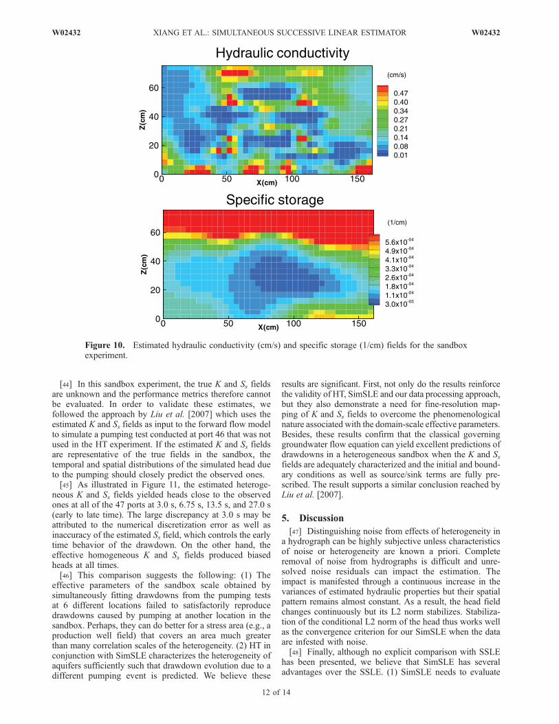
[41] A plot of variances of the estimated ln K and ln Ssfields as a function of the iteration number is illustrated inFigure 8. The variances increased continuously indicatingeffects of unresolved noise. The final estimates were chosenon the basis of the stabilization of the conditional L2 normof the head during iteration (Figure 9), which suggest thatthe best estimates are at the sixth iteration.[42] Figure 10 shows the distributions of the estimated K

and Ss fields, respectively. In Figure 10, six low-K zones inthe sandbox (Figure 7) are vividly portrayed by the esti-mated K field, but the low-K zones close to the bottom arefuzzy. The low resolution at the bottom is due to the no-fluxboundary at the bottom where the flow generally follows theboundary, and where the pressure excitations were notsampled because of absence of monitoring ports betweenthe low-K zones and the bottom boundary–consistent withfindings by Illman et al. [2007, 2008] and Liu et al. [2007].[43] The estimated Ss field in Figure 10 on the other hand

does not reflect the pattern of the K field. Rather, the fieldreflects an overall trend that the Ss values of the medium atthe bottom are smaller than those on the top. This patternappears to be physically correct: sands at the bottom arecompressed more because of greater overlying materials.The result is also consistent with the estimated Ss field fromthe analysis of cross-hole aquifer tests by Liu et al. [2007].

Figure 8. Variances of estimated ln K and ln Ss as afunction of iteration for the sandbox experiment.

Figure 9. Conditional L2 norm of the head as a functionof iteration for the sandbox experiment.

W02432 XIANG ET AL.: SIMULTANEOUS SUCCESSIVE LINEAR ESTIMATOR

11 of 14

W02432

[44] In this sandbox experiment, the true K and Ss fieldsare unknown and the performance metrics therefore cannotbe evaluated. In order to validate these estimates, wefollowed the approach by Liu et al. [2007] which uses theestimated K and Ss fields as input to the forward flow modelto simulate a pumping test conducted at port 46 that was notused in the HT experiment. If the estimated K and Ss fieldsare representative of the true fields in the sandbox, thetemporal and spatial distributions of the simulated head dueto the pumping should closely predict the observed ones.[45] As illustrated in Figure 11, the estimated heteroge-

neous K and Ss fields yielded heads close to the observedones at all of the 47 ports at 3.0 s, 6.75 s, 13.5 s, and 27.0 s(early to late time). The large discrepancy at 3.0 s may beattributed to the numerical discretization error as well asinaccuracy of the estimated Ss field, which controls the earlytime behavior of the drawdown. On the other hand, theeffective homogeneous K and Ss fields produced biasedheads at all times.[46] This comparison suggests the following: (1) The

effective parameters of the sandbox scale obtained bysimultaneously fitting drawdowns from the pumping testsat 6 different locations failed to satisfactorily reproducedrawdowns caused by pumping at another location in thesandbox. Perhaps, they can do better for a stress area (e.g., aproduction well field) that covers an area much greaterthan many correlation scales of the heterogeneity. (2) HT inconjunction with SimSLE characterizes the heterogeneity ofaquifers sufficiently such that drawdown evolution due to adifferent pumping event is predicted. We believe these

results are significant. First, not only do the results reinforcethe validity of HT, SimSLE and our data processing approach,but they also demonstrate a need for fine-resolution map-ping of K and Ss fields to overcome the phenomenologicalnature associated with the domain-scale effective parameters.Besides, these results confirm that the classical governinggroundwater flow equation can yield excellent predictions ofdrawdowns in a heterogeneous sandbox when the K and Ssfields are adequately characterized and the initial and bound-ary conditions as well as source/sink terms are fully pre-scribed. The result supports a similar conclusion reached byLiu et al. [2007].

5. Discussion

[47] Distinguishing noise from effects of heterogeneity ina hydrograph can be highly subjective unless characteristicsof noise or heterogeneity are known a priori. Completeremoval of noise from hydrographs is difficult and unre-solved noise residuals can impact the estimation. Theimpact is manifested through a continuous increase in thevariances of estimated hydraulic properties but their spatialpattern remains almost constant. As a result, the head fieldchanges continuously but its L2 norm stabilizes. Stabiliza-tion of the conditional L2 norm of the head thus works wellas the convergence criterion for our SimSLE when the dataare infested with noise.[48] Finally, although no explicit comparison with SSLE

has been presented, we believe that SimSLE has severaladvantages over the SSLE. (1) SimSLE needs to evaluate

Figure 10. Estimated hydraulic conductivity (cm/s) and specific storage (1/cm) fields for the sandboxexperiment.

12 of 14

W02432 XIANG ET AL.: SIMULTANEOUS SUCCESSIVE LINEAR ESTIMATOR W02432

the adjoint state equation only once for a given observationlocation using newly estimated hydraulic property fieldsfrom all pumping tests since the adjoint state equation isindependent of the pumping rate and pumping location. Onthe other hand, using SSLE, one must solve the adjoint stateequation for each pumping test because the parameters inthe adjoint state equation are modified for each pumpingtest. (2) SimSLE avoids the loop iteration of SSLE, and thecomputational effort is thus reduced. (3) Adding data sets indifferent sequences in SSLE may lead to a slightly differentfinal result, which is more sensitive to the last data set [seeIllman et al., 2008]. This problem does not exist in SimSLE.(4) SimSLE uses all observations simultaneously, providingmore constrains for the inverse problem and thus convergesfaster than SSLE.[49] The disadvantages of SimSLE are as follows:

(1) Since all head data sets are used simultaneously andthe same convergence criteria are applied to reach the finalestimate in SimSLE, one bad data set may affect the overallquality of the estimate. Note that both SimSLE and SSLEresult in the same estimate if the data sets are free of errors.

(2) The memory requirement is greater because the sizes ofcovariance matrix of h and the cross-covariance matrix of fand h are larger than the corresponding matrices in SSLE.

6. Conclusion

[50] Results of this study show the following: (1) in spite ofnoise in hydrographs from a HT survey, the least squaresapproach can satisfactorily estimate effective hydraulic prop-erties of the synthetic aquifer with hierarchical heterogeneitybecause the inverse problem is well posed. (2) Accurateestimation of spatial variances of K and Ss from HT data isdifficult because of the nonstationary nature of the flow field,which demands a large amount of head data to obtainrepresentative sample head variances. (3) For ill-posedproblems, HT in conjunction with our SimSLE yield satis-factory estimates of the hierarchical K and Ss fields of thesynthetic aquifer. If hydrographs are corrupted with noise,the SNR is a useful measure of reliability of a corruptedhydrograph, and wavelet denoising the hydrographs is aviable means to improve the estimate. In addition, the use ofstabilization of the conditional L2 norm of head as a

Figure 11. Validation results: observed versus estimated heads (cm) at the 47 observation ports at fourdifferent times in the sandbox. Two simulated heads were considered: one using estimated effective Kand Ss fields from the equivalent homogeneous domain and the other using the estimated heterogeneousK and Ss fields derived from the analysis of HT.

W02432 XIANG ET AL.: SIMULTANEOUS SUCCESSIVE LINEAR ESTIMATOR

13 of 14

W02432

convergence criterion in SimSLE avoids overexploitation ofnoisy data. (4) HT surveys delineate detailed hydraulicheterogeneity in aquifers, which can be used to predictdifferent flow scenarios. That is, the estimate hydraulicproperties do not suffer from the phenomenological natureassociated with the domain-scale effective properties. Fi-nally, simultaneous inclusion of hydrographs from allpumping tests in the analysis offers some advantages overthe previous sequential approach but it suffers from therequirement of huge computational resources.

[51] Acknowledgments. The second author would like to acknowledgesupport from the National Cheng-Kung University during his visits in 2006,2007, and 2008. Support from the Strategic Environmental Research andDevelopment Program (SERDP) subcontracted through the University of Iowaas well as funding from the National Science Foundation (NSF) through grantsEAR-0229717, IIS-0431079, and EAR-0450388 are acknowledged.We thankconstructive and insightful suggestions by Anna Michalak, Walter Illman, andtwo anonymous reviewers as well as Resta Cheng for proofreading themanuscript.

ReferencesBakr, A. A., L. W. Gelhar, A. L. Gutjahr, and J. R. MacMillan (1978),Stochastic analysis of spatial variability in subsurface flows: 1. Compar-ison of one- and three-dimensional flows, Water Resour. Res., 14(2),263–271, doi:10.1029/WR014i002p00263.

Barrash, W., and T. Clemo (2002), Hierarchical geostatistics and multifaciessystems: Boise Hydrogeophysical Research Site, Boise, Idaho, WaterResour. Res., 38(10), 1196, doi:10.1029/2002WR001436.

Bohling, G. C., X. Zhan, J. J. Butler Jr., and L. Zheng (2002), Steady shapeanalysis of tomographic pumping tests for characterization of aquiferheterogeneities, Water Resour. Res., 38(12), 1324, doi:10.1029/2001WR001176.

Bohling, G. C., J. J. Butler Jr., X. Zhan, and M. D. Knoll (2007), A fieldassessment of the value of steady shape hydraulic tomography for char-acterization of aquifer heterogeneities, Water Resour. Res., 43, W05430,doi:10.1029/2006WR004932.

Brauchler, R., R. Liedl, and P. Dietrich (2003), A travel time based hy-draulic tomographic approach, Water Resour. Res., 39(12), 1370,doi:10.1029/2003WR002262.

Fienen, M. N., T. Clemo, and P. K. Kitanidis (2008), An interactive Bayesiangeostatistical inverse protocol for hydraulic tomography, Water Resour.Res., 44, W00B01, doi:10.1029/2007WR006730.

Gottlieb, J., and P. Dietrich (1995), Identification of the permeability dis-tribution in soil by hydraulic tomography, Inverse Probl., 11, 353–360,doi:10.1088/0266-5611/11/2/005.

Hagen, A. (2003), Fuzzy set approach to assessing similarity of categoricalmaps, Int. J. Geogr. Inf. Sci. , 17(3), 235 – 249, doi:10.1080/13658810210157822.

Illman, W. A., X. Liu, and A. Craig (2007), Steady-state hydraulic tomo-graphy in a laboratory aquifer with deterministic heterogeneity: Multi-method and multiscale validation of K tomograms, J. Hydrol., 341(3–4),222–234, doi:10.1016/j.jhydrol.2007.05.011.

Illman, W. A., A. J. Craig, and X. Liu (2008), Practical issues in imaginghydraulic conductivity through hydraulic tomography, Ground Water,46(1), 120–132, doi:10.1111/j.1745-6584.2007.00374.x.

Kitanidis, P. K. (1995), Quasi-linear geostatistical theory for inversing,Water Resour. Res., 31(10), 2411–2420, doi:10.1029/95WR01945.

Kuhlman, K. L., A. C. Hinnell, P. K. Mishra, and T.-C. J. Yeh (2008),Basin-scale transmissivity and storativity estimation using hydraulictomography, Ground Water, 46(5), 706–715, doi:10.1111/j.1745-6584.2008.00455.x.

Li, W., A. Englert, O. A. Cirpka, J. Vanderborght, and H. Vereecken (2007),Two-dimensional characterization of hydraulic heterogeneity by multiplepumping tests, Water Resour. Res., 43, W04433, doi:10.1029/2006WR005333.

Li, W., A. Englert, O. A. Cirpka, and H. Vereecken (2008), Three-dimen-sional geostatistical inversion of flowmeter and pumping test data,Ground Water, 46(2), 193–201, doi:10.1111/j.1745-6584.2007.00419.x.

Liu, S., T.-C. J. Yeh, and R. Gardiner (2002), Effectiveness of hydraulictomography: Sandbox experiments, Water Resour. Res., 38(4), 1034,doi:10.1029/2001WR000338.

Liu, X., W. A. Illman, A. J. Craig, J. Zhu, and T.-C. J. Yeh (2007), La-boratory sandbox validation of transient hydraulic tomography, WaterResour. Res., 43, W05404, doi:10.1029/2006WR005144.

Mallat, S. (1999), A Wavelet Tour of Signal Processing, 577 pp., Academic,San Diego, Calif.

Press, W. H., S. A. Teukolsky, W. T. Vetterling, and B. P. Flannery (1992),Numerical Recipes in FORTRAN 77: The Art of Scientific Computing,933 pp., Cambridge Univ. Press, New York.

Straface, S., T.-C. J. Yeh, J. Zhu, S. Troisi, and C. H. Lee (2007), Sequentialaquifer tests at a well field, Montalto Uffugo Scalo, Italy, Water Resour.Res., 43, W07432, doi:10.1029/2006WR005287.

Tosaka, H., K. Masumoto, and K. Kojima (1993), Hydropulse tomographyfor identifying 3-D permeability distribution, in Proceedings of the 4thAnnual International Conference on High Level Radioactive Waste Man-agement; Apr 26–30 1993; Las Vegas, NV, USA, High Level RadioactiveWaste Management, edited by B. M. Cole, pp. 955–959, Am. Soc. ofCiv. Eng., New York.

Vasco, D. W., H. Keers, and K. Karasaki (2000), Estimation of reservoirproperties using transient pressure data: An asymptotic approach, WaterResour. Res., 36(12), 3447–3465, doi:10.1029/2000WR900179.

Vesselinov, V. V., S. P. Neuman, andW. A. Illman (2001), Three-dimensionalnumerical inversion of pneumatic cross-hole tests in unsaturated fracturedtuff: 1. Methodology and borehole effects, Water Resour. Res., 37(12),3001–3017, doi:10.1029/2000WR000133.

Wu, C.-M., T.-C. J. Yeh, J. Zhu, T. H. Lee, N.-S. Hsu, C.-H. Chen, and A. F.Sancho (2005), Traditional analysis of aquifer tests: Comparing apples tooranges?,Water Resour. Res., 41, W09402, doi:10.1029/2004WR003717.

Ye, M., R. Khaleel, and T.-C. J. Yeh (2005), Stochastic analysis of moistureplume dynamics of a field injection experiment, Water Resour. Res., 41,W03013, doi:10.1029/2004WR003735.

Yeh, T.-C. J., and S. Liu (2000), Hydraulic tomography: Development of anew aquifer test method, Water Resour. Res., 36(8), 2095 – 2105,doi:10.1029/2000WR900114.

Yeh, T.-C. J., R. Srivastava, A. Guzman, and T. Harter (1993), A numericalmodel for two dimensional flow and chemical transport, Ground Water,31(4), 634–644, doi:10.1111/j.1745-6584.1993.tb00597.x.

Yeh, T.-C. J., M. Jin, and S. Hanna (1996), An iterative stochastic inversemethod: Conditional effective transmissivity and hydraulic head fields,Water Resour. Res., 32(1), 85–92, doi:10.1029/95WR02869.

Yeh, T.-C. J., C.-H. Lee, K.-C. Hsu, and Y.-C. Tan (2007), Fusion of activeand passive hydrologic and geophysical tomographic surveys: The futureof subsurface characterization, in Data Integration in Subsurface Hydrol-ogy, Geophys. Monogr. Ser., vol. 171, edited by D. W. Hyndman, F. D.Day-Lewis, and K. Singha, pp. 109–120, AGU, Washington, D. C.

Zhang, Q., R. Aliaga-Rossel, and P. Choi (2006), Denoising of gamma-raysignals by interval-dependent thresholds of wavelet analysis, Meas. Sci.Technol., 17, 731–735, doi:10.1088/0957-0233/17/4/019.

Zhu, J., and T.-C. J. Yeh (2005), Characterization of aquifer heterogeneityusing transient hydraulic tomography, Water Resour. Res., 41, W07028,doi:10.1029/2004WR003790.

Zhu, J., and T.-C. J. Yeh (2006), Analysis of hydraulic tomography usingtemporal moments of drawdown-recovery data, Water Resour. Res., 42,W02403, doi:10.1029/2005WR004309.

K.-C. Hsu and C.-H. Lee (corresponding author), Department of

Resources Engineering, National Cheng Kung University, Tainan, 701,Taiwan. (leech@mail.ncku.edu.tw)

J.-C. Wen, Department of Environmental and Safety Engineering,Research Center for Soil and Water Resources and Natural DisasterPrevention, National Yunlin University of Science and Technology, Touliu,Yunlin, 64045, Taiwan.

J. Xiang and T.-C. J. Yeh, Department of Hydrology and WaterResources, University of Arizona, Tucson, AZ 85721-0001, USA.

14 of 14

W02432 XIANG ET AL.: SIMULTANEOUS SUCCESSIVE LINEAR ESTIMATOR W02432