A Review of Urban Computing for Mobile Phone Traces ...ares.lids.mit.edu/fm/documents/review.pdfA...

A Review of Urban Computing for Mobile Phone Traces:Current Methods, Challenges and Opportunities

Shan JiangDepartment of Urban Studies

and PlanningMassachusetts Institute of

Technology, Cambridge, [email protected]

Gaston A. FioreDepartment of Aeronautics

and AstronauticsMassachusetts Institute of


Yingxiang YangDepartment of Civil and

Environmental EngineeringMassachusetts Institute of


Joseph Ferreira, Jr.Department of Urban Studies

and PlanningMassachusetts Institute of


Emilio FrazzoliDepartment of Aeronautics

and AstronauticsMassachusetts Institute of


Marta C. GonzálezDepartment of Civil and

Environmental EngineeringMassachusetts Institute of


ABSTRACTIn this work, we present three classes of methods to extrac-t information from triangulated mobile phone signals, anddescribe applications with different goals in spatiotemporalanalysis and urban modeling. Our first challenge is to re-late extracted information from phone records (i.e., a set oftime-stamped coordinates estimated from signal strengths)with destinations by each of the million anonymous users.By demonstrating a method that converts phone signals in-to small grid cell destinations, we present a framework thatbridges triangulated mobile phone data with previously es-tablished findings obtained from data at more coarse-grainedresolutions (such as at the cell tower or census tract levels).In particular, this method allows us to relate daily mobilitynetworks, called motifs here, with trip chains extracted fromtravel diary surveys. Compared with existing travel demandmodels mainly relying on expensive and less-frequent travelsurvey data, this method represents an advantage for apply-ing ubiquitous mobile phone data to urban and transporta-tion modeling applications. Second, we present a methodthat takes advantage of the high spatial resolution of thetriangulated phone data to infer trip purposes by examiningsemantic-enriched land uses surrounding destinations in in-dividual’s motifs. In the final section, we discuss a portablecomputational architecture that allows us to manage andanalyze mobile phone data in geospatial databases, and tomap mobile phone trips onto spatial networks such that fur-ther analysis about flows and network performances can bedone. The combination of these three methods demonstratethe state-of-the-art algorithms that can be adapted to tri-angulated mobile phone data for the context of urban com-puting and modeling applications.

KeywordsMobile Phones, Human Mobility, Human Activity, LandUse, Spatial Networks, GPS, Spatiotemporal Computation,Boston.______________________________Permission to make digital or hard copies of all or part of this work forpersonal or classroom use is granted without fee provided that copies are notmade or distributed for profit or commercial advantage and that copies bearthis notice and the full citation on the first page. Copyrights for componentsof this work owned by others than ACM must be honored. Abstracting withcredit is permitted. To copy otherwise, or republish, to post on servers or toredistribute to lists, requires prior specific permission and/or a fee. Requestpermissions from [email protected].

UrbComp’13, August 11–14, 2013, Chicago, Illinois, USA.Copyright© 2013 ACM 978-1-4503-2331-4/13/08 ...$15.00

1. INTRODUCTIONThe emergent field of Urban Computing seeks to develop

computational solutions that make cities more livable, moreefficient, and better positioned for the centuries ahead [2].An important aspect in this endeavor is to have good reliableestimates of when and how the millions of individuals thatcohabit a metropolis use their facilities. These daily set ofindividual choices are very diverse and difficult to infer inurban populations. One reason for this difficulty lies in thestochasticity of the options for activity types, travel modes,routes, sequences, and trip purposes that an individual canmake in a given city. However, despite some degree of changeand spontaneity, human mobility is, in fact, characterized bya deep-rooted regularity that allows us to detect predictabletrends of urban dynamics [43, 42, 19, 15, 4].

Increasing storage capacity and processor clouds makepossible to capture petabytes of digital traces from individu-al activities worldwide. Internet usage, credit card transac-tions, GPS-equipped vehicles, subway smart cards, amongothers, save in the cloud our time-stamped coordinates everytime we use them [28, 14, 38]. But few things are better sen-sors of our daily whereabouts than our mobile phones [27].A mobile phone tracks our location every time we text, callor web browse; and even passively when it communicates tothe cellular network access points. The recently improvedability to capture, store, and understand massive amountsof data is changing the methods for inferring human behav-ior [13]. As our data collection grows, so will the opportunityto find better methods to interpret and transmit the data ina world where people and machines are more interconnected.

The dynamics of a population’s daily movement is a com-plex system; still, there are several non-trivial features thathave been measured independently of the specific details ofthe urban group. These features are called universal in anal-ogy with reproducible phenomena that appear in the naturalsciences. Basic and common mechanisms are responsible forthe presence of each of those ubiquitous features in systemsgoverned by human activity. One widespread example thatuses these universal approaches includes gravity-like modelsto estimate the aggregate statistic in mobility and migra-tion among populations. It has been proved that a simplestochastic process can capture local mobility decisions thathelp us derive analytically commuting and mobility fluxes,requiring as an input-only information on the distributionof population and facilities [41] without details about indi-vidual demographics, socioeconomics or activity types. Theeffectiveness of this simplified model stems from the highcorrelation that exists among the aforementioned distribu-

tions and the resulting production and attraction of trips indiverse populations.

The findings of other kinds of essential characteristics inurban mobility serve as a powerful way to convert passivedata into useful models that help city planning. In thiswork, we will present methods that capture generalizablepatterns not in aggregated but in individual trips. Our goalis two-fold. First, we will review and illustrate some of the u-biquitous findings in human mobility, as captured by mobilephone data or travel surveys, introducing the methodolo-gy to treat the data. Second, we will present the currentcomputational challenges involved in treating these data forinferring trip purposes and road usage.

The first universal feature that we will explore is the pres-ence of preferential returns to visited locations mixed withthe exploration of new ones [42, 43]. The frequent return topreviously visited locations is captured by the average in-crease in the number of visited places over time as a resultof the exploration behavior to seek for new locations mixedwith the tendency for revisiting locations [42, 19]. Generalfindings for individual urban motion have to contain thesetwo principles that govern human mobility. A particularchallenge in this paper is how to reconcile previous findingsobserved at more aggregate spatial scales, such as use ofsubway stations [19] or mobile phone towers, with triangu-lated mobile phone data sets containing thousands of noisycoordinates per individual user [42, 29].

A second feature that we will measure from the triangulat-ed mobile phone data is the extraction of daily mobility mo-tifs. The organization of daily trips have revealed ubiquitousconfigurations that can be expressed as daily networks withnodes representing locations and directed edges represent-ing trips. The same distribution of trip configurations hasbeen found in different cities, and measured by both travelsurveys and mobile phone data [39]. Individuals make dailytrips to five or fewer locations using only 17 of the more than1 million possible network configurations. The basic mech-anism generating these networks is the circadian rhythm ofour daily movement and a perturbation factor expressed ina hidden Markov model. This factor implies that once in-dividuals are engaged in a single flexible activity that lastsat least 30 minutes, they are 10 times more likely to engagein an additional flexible activity that day, compared withthose people who have not yet left a fixed activity, such asthe workplace or home. The prevalence of the 17 trip con-figurations indicates that they represent “motifs”, which arenetwork patterns occurring with such frequency that the sta-tistical probability of their random occurrence is negligible.The presence of motifs indicates a basic principle that canbe used in predictive models of daily trip chains. Here weshow how to detect the stay points from triangulated mobilephone records that give rise to the daily motifs.

In the paper, we analyze triangulated mobile phone record-s for the Boston metropolitan area as a demonstration. InSections 2 and 3, we present the data characteristics and therequired computational methods to extract the two knownuniversal features of individual trips (i.e., the explorationscombined with preferential returns), as well as the dailymobility motifs compared with the travel survey data forBoston metropolitan area [32]. In Section 4, we discuss themethods and current challenges of how to combine the ex-tracted urban mobility features with land use informationto infer activities and types of destinations associated withthese trips. In Section 5, we present the methods to matchtrips captured by phones onto the spatial network. Ourgoal is to develop methods to reproduce previous findingson road usage with a platform that is computationally in-tegrated and publicly available. The results presented hereserve as a starting point for unified methods of analysis togreatly simplify the dimensionality of the data by captur-ing the essence of the information and reducing details thatwould generate overfitting. These outcomes enable convert-ing these data into valuable information with great benefitsfor urban applications.

2. DATA DESCRIPTION AND PREPROCESS-ING

Our dataset contains 834,690,725 anonymized mobile phonerecords from 1 million users in the Boston metropolitan area(around 19.35% of the population, from several carriers) fora period of two months in 2010. Each record contains anony-mous User ID, longitude, latitude, and time stamp of thephone activity. The coordinates of the records are estimat-ed by a standard triangulation algorithm (and the data donot include cell phone tower information). The accuracy ofthe location is about 200- to 300- meters, which is of higherresolution than representing locations by cell towers [44, 42,5]. This finer granularity enables us to identify locations ofusers more accurately and thus to adapt data preprocessingmethods that have been previously applied to GPS records[48, 47, 49, 17].

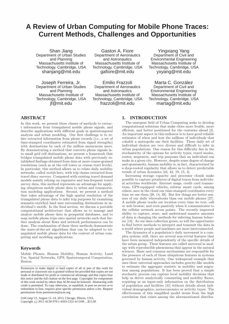
The first step in the data preprocessing is to identify stays(i.e., phone records made when users are engaging in activi-ties) and pass-by’s (i.e., records made during travelling) fromeach user’s trajectory. As illustrated in Fig. 2.1, a stay-pointis identified by a sequence of consecutive cell phone recordsbounded by both temporal and spatial constraints. The spa-tial constraint is the roaming distance when a user is stayingat a location, which should be related to the accuracy of thedevice collecting location data. In this study we set theroaming distance as 300 meters. The temporal constraintis the minimum duration spent at a location, which is mea-sured as the temporal difference between the first and thelast record in a stay. In this study, only records meeting thespatial constraint criterion and with duration more than 10minutes are counted as stays. Once a stay point is identified,its location is set as the centroid of all records belonging tothat stay. In Fig. 2.1 s1 is the centroid of p3, p4, and p5.

p1

p2

p3p4

p5

p6s1

s2s3

p7

r1

cell recordstay point

stay region

Figure 2.1: Illustration of the data preprocessingprocess. The green points are raw triangulated cellphone records. The red points are identified stay-points. The blue point is a stay region, which is acluster of stay-points.

The next step is to identify stay-regions from stay pointssince different stay-points identified from one user’s severaldifferent trajectories may refer to a same location, but thesestay-points’ coordinates are unlikely to be exactly the same.We use a grid-based clustering method to cluster stay-pointsto get stay-regions. As shown by Zheng et. al [47] the advan-tage of the grid-based clustering method over the k-meansalgorithm and the density-based OPTICS clustering algo-rithm is that it can constrain the output cluster sizes, whichis desirable when we know that each location should havea bounded size and the accuracy of the records is within acertain range. In this study the maximum stay region sizeis set to d = 300m to approximate the area that might like-ly be traversed on foot as part of an urban activity. Theprocedure to perform grid-based clustering is to first dividethe entire region into rectangular cells of size d/3. Next tomap all the stay-points to each cell. Then iteratively mergethe unlabeled cell with the maximum stay-points and itsunlabeled neighbours to a new stay-region. Once a cell isassigned to a stay region, it is marked as labeled. For thedetailed algorithm please refer to [47]. In Fig. 2.1, the three

stay-points are clustered to one stay-region r1.

3. UNIVERSAL PATTERNS OF INDIVIDU-AL MOBILITY

3.1 Exploration and Preferential ReturnsSeveral ubiquitous characteristics of individual human tra-

jectories have been found [4, 15, 42, 5], most of which areusing tower level cell phone records. One important aspectis to measure the degrees of predictability of human mobil-ity. Previous studies [43] found that, on average, 70% ofthe time the most visited location coincides with a user’sactual location at a given time of the day. The distributionsof travel distance (P (r)), inter-activity time (P (t)), radiusof gyration (rg), location visiting frequency (fk) and loca-tion exploration probability show that human trajectoriespresent statistical regularities that can be related via scal-ing laws. The location visiting frequency usually conformsto Zipf’s law [50]. This implies a hierarchical ranking in ourvisitation patterns that relates to the exploration and pref-erential return to certain locations, which is an ubiquitousmechanism in human mobility [42]. The more locations aperson has visited, the less likely s/he is going to visit a newlocation, or in other words, the more likely s/he is going toreturn to a previously visited location. This probability isproportional to the previous visiting frequency of that loca-tion. With data at the finer granularity level available, wewould like to test wether these scaling laws still hold on thestay locations extracted as described in the previous section.

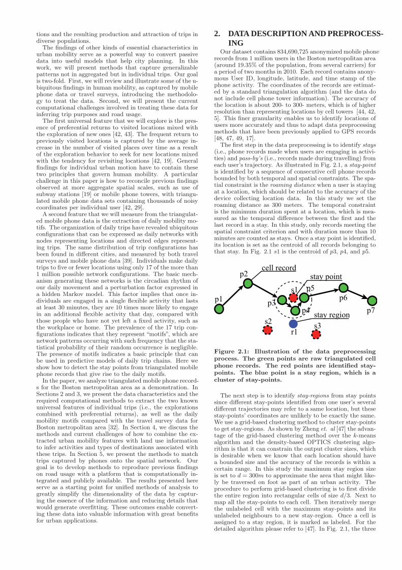
We begin our exploration by calculating the users’ mo-bility regularity R(t), which is defined as the probability offinding the user in her/his most visited location at hourlyinterval in a week. Fig. 3.1(a) shows that, under finer gran-ularity, there is a regularity for all users in a week. Theaverage regularity drops from 70% (in tower level data) to64% measured at the level of stay cells. As expected, theregularity is still higher during night and lower during theday. It’s also higher during weekends. The average numbersof visited locations, for all the users in each hour of a week,show exactly the opposite pattern of R.

Next, we examine how the users explore different location-s. The number of distinct locations visited over time, S(t)follows the following trend:

S(t) ∼ tµ, (1)

where µ = 0.6 ± 0.02 for tower-level cell phone data [42].Fig. 3.1(b) shows how S(t) vs. t changes for user groupsthat visited a different number of locations during the two-month period. As can be expected, user groups that visitedmore locations in the two-month period have higher slopes.For group s : 80− 100, µ = 0.66 while for group s : 20− 40,µ = 0.41. For all the users µ = 0.59, which agrees withprevious findings.

Next, we measure the visiting frequency f of the kth mostvisited locations, which follows the shape: fk ∼ k−ξ, withξ = 1.04 (Fig. 3.1(c)), which is slightly smaller than theone observed with higher granularity data, of ξ = 1.2; themulti-scale effects still deserve more thorough investigationand may be sensitive to the scale of stay regions.

Fig. 3.1(d) shows that if a user returns to a previouslyvisited location, the probability Π to return to that locationis proportional to that location’s previous visiting frequencyf . This evidence again supports the exploration and prefer-ential return mechanism in human mobility.

3.2 Daily MotifsIndividual daily mobility is well described by activity chain-

s that include the start time, the end time, and the locationof each activity within a day. Activity chains are usual-ly obtained from travel survey data, which is accurate butwith low sampling rate (around 1% of total households ina metropolitan area) and usually records only one day oftravel dairies per household [23]. Cell phone data has theopposite characteristics: not all stays in a day can be cap-

100

101

102

100

101

102

t(h)

S(t

)

s: 20−40s: 40−60s: 60−80s: 80−100

~ t~ t~ t~ t

0.66

0.59

0.52

0.41

100

101

10210

−3

10−2

10−1

100

k

f k

s: 20−40s: 40−60s: 60−80

s: 80−100

~ k-1.04

0 0.1 0.2 0.3 0.4 0.50

0.1

0.2

0.3

0.4

0.5

f

Π

b

c

0.5

0.6

0.7

0.8

Time(t)

R(t

)

M T W T F S S

d

a

Figure 3.1: Scaling laws of human dynamics. (a)The users’ mobility regularity R is higher duringnight and lower during day with the average val-ue 64%. (b) The number of distinct visited locationsS(t) follows S(t) ∼ tµ with µ = 0.66 for group s : 80−100and µ = 0.41 for group s : 20 − 40. (c) User groupswith different numbers of visited locations have thesame fk distribution: fk ∼ k−1.04, which is similarto previous findings using larger spatial granularity[15, 42, 19]. (d) The probability Π to return to alocation is proportional to that location’s previousvisitation frequency f .

tured in the cell phone data, but it has much longer periodsof sampling over larger fractions of the population–in thisstudy it contains 20% of the population in Boston over a 2month period. So a question arises: can the larger volumeand longer periods of observation make up for the less accu-racy in the cell phone data? We find that this is the case ifthe data is filtered in a proper way.

Larger volume of data enables us to filter out the noiseand select only users with enough information for detectingdaily trip chains. The sampling method requires: (1) To se-lect only frequent cell phone users with enough records; (2)To remove pass-by points which are only used during trav-el; (3) To eliminate signal transitions between neighboringlocations; (4) To detect individual trips only for days withat least 7 identifiable time-slot locations (a day is dividedinto 48 half hour slots); (5) To overcome the small numberof night calls, the location which is visited most frequentlyduring all nights between 12 am and 6 am of a single user, isassigned to be the user’s home location. For a detailed de-scription of the filtering process please refer to our previousstudy [39].

For each sampled individual trajectory, we construct atravel network in which nodes represent the visited stay-regions and directed edges stand for trips between them.We count the statistically significant configurations in thedata sets, which are called motifs, adopting the term fromnetwork science [31]. This notion is similar to the notionof activity chains. The difference is that here we distin-guish locations by the coordinates of the stay-region ratherthan the functionality of the location such as home, work,etc. This formulation is suitable for passive observationsof mobile phone data in which we have higher degrees ofuncertainty inferring trip purposes.

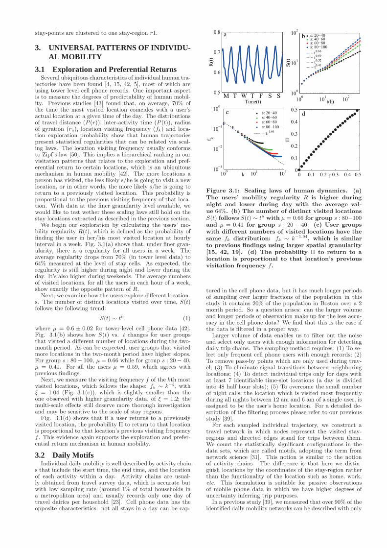
In a previous study [39], we measured that over 90% of theidentified daily mobility networks can be described with only

17 different motifs. We test this finding here by extractingmotifs for both cell phone users in our dataset and from the2010/2011 Massachusetts travel survey [32], which contains37, 023 people’s travel dairy over one day on a rolling ba-sis. Fig. 3.2 shows the distributions of the 17 motifs whichare similar for the two different data sources, and they alsoagree with the previous findings measured in Chicago andParis. This result shows the validity of the proposed methodfor triangulated cell phone data, which presents a good al-ternative for analyzing daily human mobility patterns andcomplements expensive surveys.

1 2 3 4 5 6 7 8 9 10 11 12 13 14 15 16 170%

10%

20%

30%

40%

motif ID

P(I

D)

Phone

Survey

Figure 3.2: Frequent daily motifs. The 17 most fre-quent motifs account for over 90% of the measureddaily trips. The distributions of the 17 motifs ex-tracted from cell phone data and the Massachusettstravel survey are similar, and also conform to previ-ous findings in Paris and Chicago [39].

4. INFERRING INDIVIDUAL ACTIVITIESAND TRAVEL

To make the million users’ mobile phone traces usefulfor urban land use, community planning and transportationplanning, it is crucial to answer one of the most importantquestions: “What are people doing in space and time?” [1,6, 16, 30, 24, 25, 26]. This question includes inferring thespatiotemporal activities that people engage in, and theirtravel (e.g., trip chaining, and road usage, etc.) induced bythe needs of pursuing activities [35].

In order to infer the types and patterns of activities ofanonymous individuals, by learning their historical presencein space and time and characteristics of their destinations(e.g., land use, points-of-interest (POIs)), we need to addressseveral challenges presented by the mobile phone records(for billing purposes) as opposed to by GPS data for whichmany algorithms and methods have been developed to studyhuman behavior [47, 17]. First, mobile phone data are per-ceived with indefinite gaps in space and time, while GPSdata are recorded with a high frequency such that they canbe treated as continuous trajectories. Second, the locationalaccuracy of mobile phone data is lower than the pinpointedGPS traces (depending on the technologies [36]).

In this section, we present a class of algorithms that aretailored to address the distinct characteristics of the mobilephone data (triangulated at 200- to 300-meter accuracy lev-el) such that we can use the filtered data to infer humanactivities and their travel in space and time. In contrastto the grid-based algorithm presented in Section 2, the onepresented here is designed to exploit the maximum spatialaccuracy possible. Comparing these two classes of data fil-tering methods is beyond the scope of this paper and willbe presented elsewhere.

4.1 Extracting Stay, Pass-by and Potential S-tay Areas

For the purpose of extracting individuals’ whereaboutsfrom phone records, including their stationary stay locations(so as to infer their activity types) and their moving pass-bylocations (so as to infer their travel path and road usage),

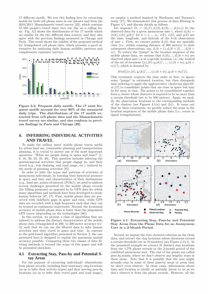
we employ a method inspired by Hariharan and Toyama’sstudy [17]. We demonstrate this process of data filtering inFigure 4.1, and discuss details as follows.

Let sequence Di = (di(1), di(2), di(3), ..., di(ni)) be theobserved data for a given anonymous user i, where di(k) =(t(k), x(k), y(k))′ for k = 1, ..., ni, t(k), x(k), and y(k) arethe time, longitude, and latitude of the k-th observationof user i. First, we extract points di(k) that are spatiallyclose (i.e. within roaming distance of 300 meters) to theirsubsequent observations, say, di(k + 1), di(k + 2), ..., di(k +m). To reduce the “jumps” in the location sequence of themobile phone data, we assume that di(k), ..., di(k + m) areobserved when user i is at a specific location, i.e., the medoidof the set of locations {(xi(k), yi(k))

′, ..., (xi(k +m), yi(k +m))′}, which is denoted by

Med({(xi(k), yi(k))′, ..., (xi(k +m), yi(k +m))′}).

This treatment respects the time order at first, to ignorenoisy “jumps” in estimated location, but then disregardstime ordering to apply the agglomerative clustering algorith-m [17] to consolidate points that are close in space but maybe far away in time. The points to be consolidated togetherform a cluster whose diameter is required to be no more thana certain threshold (set to be 500 meters). Again, we mod-ify the observation locations to the corresponding medoidsof the clusters (see Figures 4.1(a) and (b)). It turns outthat by these treatments, we greatly reduce the noise in thelocation sequences of the mobile phone data (i.e., errors insignal triangulations).

!(!(!(!(!(!(

!(!(!(!(!(!(!(!(

!(!(!(!(!(!(!(!(

!(!(!(!(!(!(!(!(!(!(!(!(!(!(!( !(!(!(!(!(!(!(!(!(!(!(!(!(!(!(!(!(!(!(

!(!(!(!(!(!(!(!(!(!(!(!(!(

!(!(!(!(!(!(!(!(!(!(!(!(!(

!(!(!(!(!(!(!(

!(!(!(!(!(!(!(

!(!(!(!(!(!(!(!(!(!(!(!(!(!(!(!(!(!(!(!(!(!(!(!(!(!(!(!(

!(!(!(

!(!(

!(!(!(!(!(!(!(!( !(!(!(!(

!(!( !(

!(!(!(

!(!(

!(

!(

!(!(

!(!( !(!(!(

!(!(

!(!(!(!(!(!(!(

!(

!(!(!(!(!(!(!(!(!(!(!(!(!(

!(!(!(!(!(!(

!(!(!(!(!(!(!(!(!(!(!(!(!(!(!(!(!(!(!(!(!(!(!(!(!(!(!(!(!(!(!(!(!(!(!(!(!(!(!(!(!(!(

!(!(!(!(!(!(!(!(!(!(!(!(!(!(!(!(!(!(!(!(!(!(!(!(

!(!(!(!(!(!(!(!(!(!(!(!(!(!(!(!(!(!(!(!(!(!(!(!(!(!(!(!(!(!(!(!(!(!(

!(!(!(

!(!(

!(

!(!(!(!(!(!(!(!(!(!(!(!(!(!(!(!(!(!(!(!(!(!(!(!(!(!(!(!(!(!(!(!(!(!(!(!(!(!(!(!(!(!(!(!(!(!(!(

!(

!(!(!(!(!(!(!(!(!(!(!(!(!(!(!(!(!(!(!(!(!(!(!(!(!(!(!(!(!(!(!(!(!(!(!(!(!(!(!(

!(!(

!(!(

!(!(!(!(!(!(!(!(!(

!(!(!(

!(

!(!(!(!(!(!(!(!(!(!(!(!(!(!(!(!(!(!(!(!(

!(!(

!(!(

!(!(!(!(!(!(!(!(!(!(!(!(!(!(!(

!(!(!(!(!(!(!(!(!(!(

!(!(!(!(!(!(!(!(!(!(!(!(!(!(!(!(!(!(!(!(!(!(!(!(!(!(!(!(!(!(!(!(!(!(!(!(

!(!(

!(!(!(!(!(!(!(!(!(!(!(

!(

!(!(!(!(!(!(!(!(

!(!(!(!(!(!(!(!(!(!(!(!(!(!(!(!(!(!(!(!(!(!(!(!(!(!(!(!(!(!(!(!(!(!(!(!(!(!(!(!(!(!(!(!(!(!(!(!(!(!(!(!(!(!(!(!(

!(

!(!(!(!(!(!(!(!(

!(!(!(!(!(!(

!(!(!(!(

!(!(!(

!(

!(!(!(!(

!(!(!(!(

!(!(!(!(!(!(!(!(!(!(!(!(!(!(!(!(!(

!(!(!(!(!(!(!(

!(!(!(!(!(

!(!(!(!(!(!(!(!(!(!(!(!(

!(!(

!(!(!(!(!(!(

!(

!(!(!(!(!(!(!(!(!(

!(!(!(!(!(!(

!(!(

!(!(

!(!(!(!(

!(!(!(

!(!(

!(!(!(!(

!(

!(!(!(

!(!(!(!(

!(!(!(!(!(!(

!(!(!(!(

!(

!(!(

!(!(!(!(!(!(!(!(

!(

!(!(

!(!(

!(!(

!( !(!(!(!(!(!(!(

!(!(!(!(!(!(!(!(!(!(

!(!(!(!(!(!(!(!(!(!(!(!(

!(!(!(!(!(

!(

!(!(

!(!(!(!(

!( !(!(!(!(

!(!(!(!(!(!(

!(!(!(!(!(

!(

!(!(!(!(!(

!(!(

!(!(

!(!(!(!(!(!(!(!(!(!(!(!(!(!(!(!(!(!(!(!(

!(!(!(!(

!(!(

!(!(

!(!(!(!(!(!(!(

!(!(

!(!(!(!(!(!(!(!(!(!(!(!(!(

!(!(!(!(!(!(!(!(

!(

!(

!(!(!(!(!(!(!(!(!(!(

!(

!(

!(!(

!(!(!(!(!(!(

!(!(!(!(!(!(!(!(!(!(

!(!(!(!(!(!(

!(!(!(!(!(!(!(!(!(!(

!(!(

!(

!(

!(

!(!(

!(

!(!(!(!(

!(!(!(!(!(!(!(!(!(!(!(!(

!(!(!(!(

!(!(

!(

!(

!(!(!(!(!(!(!(!(!(!(!(!(!(!(!(!(!(!(!(!(

!(!(

!(!(!(!(!(!(

!(!(!(!(!(!(!(!(!(!(!(!(!(!(!(!(!(!(!(!(

!(!(

!(

!( !(

!(!(!(!(

!(!(!(

!(

!(!(!(!(!(!(!(!(!(!(!(!(!(!(!(!(!(!(!(!(!(!(!(!(!(!(!(!(!(!(!(

!(!(!(!(!(!(

!(!(

!(!(

!(!(!(

!(!(

!(!(

!(

!(!(!(!(!(!(!(!(!(!(!(!(

!(!(

!(!(!(!( !(!(!(!(!(!(!(!(!(!(!(!(

!(!(!(!(!(!(!(!(!(!(

!(!(

!(!(

!(!(

!(

!(!(!(!(!(!(!(!(!(!(!(!(!(!(

!(

!(

!(!(!(!(!(!(!(!(!(!(!(

!(!(

!(!(

!(!(!(!(!(!(!(

!(!(

!(!(!(!(!(!(

!(!(

!(!(!(!(!(!(!(!(!(!(

!(

!(

!(!(!(!(

!(!(!(!(!(!(

!(!(!(

!(!(!(!(!(!( !(!(!(!(!(!(!(!(!(!(

!(!(

!(!(

!(!(

!(

!(!(

!(!(!(!(

!(

!(

!(!(!(!(!(

!(!(!(

!(!(!(!(!(!(!(!(!(

!(

!(!(

!(!(

!(!(!(!(!(!(!(!(

!(!(!(!(!(

!(!(

!(

!(!(!(!(!(!(!(!(!( !(!(!(!(!(!(!(!(!(!(!(!(!(!(!(!(!(!(!(!(!(!(!(!(

!(

!(!(!(!(!(!(!(!(!(!(!(!(!(!(!(!(!(

!(

!(!(!(!(!(!(!(!(

!( !(

!(

!(!(!(!(

!(

!(!(

!(!(!(!(!(!(

!(!(!(!(!(!(!(!(!(!(!(!(!(!(!(!(!(!(!(!(!(!(!(!(

!(!(!(!(!(!(

!(!(!(!(!(!(!(!(!(!(

!(!(!(!(!(!(!(!(

!(

!(!(

!(!(!(!(!(!(!(!(!(!(!(!(!(!(!(!(!(!(!(!(!(

!(!(

!(!(!(!(!(!(!(!(!(!(!(!(!(!(!(!(!(!(!(!(!(!(!(!(!(!(!(!(

!(!(

!(

!(

!(!(!(!(!(!(!(!(!(!(!(!(!(!(!(!(!(!(!(!(!(!(!(!(!(!(!(

!(!(

!(

!(

!(

!(!(!(!(

!(!(!(!(

!(!(!(!(!(!(!(!(!(!(!(!(!(!(

!(

!(!(

!(!(!(!(!(!(!(!(!(!(!(!(!(!(!(!(!(!(!(!(

!(!(!(

!(!(

!(!(

!(!(!(!(!(!(!(!(

!(

!(!(

!(!(

!(!(

!(!(!(!(!(!( !(!(

!(!(!(!(!(!(!(!(!(!(!(!(!(!(!(!(!(

!(!(!(!(!(!(!(!(

!(

!(

!(!(!(!(!(!(!(

!(!(

!(!(

!(!(!(!(!(!(!(!(!(!(!(!(

!(!(

!(

!(

!(

!(!(!(!(

!(!(!(!(!(!(!(!(!(!(!(

!(!(!(!(!(!(!(!(!(!(!(!(!(!(!(!(!(!(!(!(!(!(!(!(!(!(

!(!(

!(!(

!(!(

!(!(!(!(!(!(!(!(!(!(!(!(!(!(!(!(!(!(!(!(!(!(!(!(!(

!(!(!(!(

!(!(

!(!( !(!(!(

!(!(

!(

!(!(!(!(!(!(!(

!(!(!(!(!(

!(!(

!(!(!(!(!(!(!(!(!(!(!(

0 9 18 27 36Kilometers

!(!(!(!(!(!(

!(!( !(!(

!(!(!(!(

!(!(!(

!(

!(

!(!(

!(

!(!(!(!(!(!(!(!(

!(

!(!(!(!(!(

!( !( !(!(!(!(!(!(!(!(

!(

!(!(!(!(!(!(

!(

!(

!(

!( !(!(!(!(!(!(!(!(!(

!(

!(!(

!(!(!(!(!(!(!(!(!(!(

!(!(!(

!(!(

!(!(

!(!(!(

!(!(!(!(!(!(

!(

!(!(!(!(!(!(!(!(!( !(!(

!(!(!(!(!(!(!(!(!( !(!(!(!(

!(!(

!(!(

!(!(

!(!( !(!(

!(!(

!(!(

!(

!(!(!(!(

!(

!( !(

!( !(

!(

!(!(

!(

!(

!(!(

!(!(!(!(!(

!(!(

!(

!(!(!(!(!(

!(

!(

!(!(!(!(!(!(!(

!(

!(!(!(!( !(

!(

!(!(!(!(!(

!(!(!(!(!(!(!(!(!(!(!(!(!(

!(!(!(!(!(!(!(!(!(!(

!(

!(!(!(!(!(!(!(

!(!(!(

!(

!(

!(

!(!(!(!(!(

!(!(!(!(!(!(

!(!(

!(!( !(!(!(!(!(!(!(!(!(!( !(!(

!(!(

!(!(!(!(

!(

!(

!(!(

!(

!(

!(

!(

!(!(!(

!(

!(!(!(!(!(!(

!(

!(

!(!(

!(!(!(!(

!(!(!(!(

!(!(

!(

!(

!(

!(

!( !(!(!(!(!(!( !(

!(!(

!(!(!(!(!(

!(

!(!(!(!(!(

!( !(!(!(

!(!(!(

!(

!(!(!(!( !(!(!(!(!(

!(

!(!(!(!(!(!(!(!(

!(

!(

!(!(!(!(!(!(

!(!(!(!(!(!(!(!(

!(!(!(!(!(!(!(!( !(!(!(!(!(!(!(!( !(!(!(!(!(!(!(!(

!(!(

!(!(

!(!(

!(

!(!(!(!(

!(!(

!(

!(!(

!(

!(

!(!(

!(!(!(!(!(!(

!( !(

!(

!(!(

!(!(

!(

!(

!(!(

!(

!(

!(

!(

!(!(!(

!(

!(!(!(!(!(!(!(!(!(!(!(

!(!(!(!(!(!(!(!(!(

!(

!(!(!(!(!(!(!(!(!(!(!(!(!(!(!(!(!(!(!(!(!(!( !(!(

!(!(!(!(!(!(!(!(

!(!(

!(!(

!(!(

!(!(!(!(!(!(!(

!(

!(

!(

!(!(!(!(!(!(!(!(!(!(!(!(!(!(!(!( !(!(!(!(!(!(!(!(!(!(!(!(!(!(!(!(!(!(!(!(!(!(!(!(!(!(!(!(!(!(

!(

!(!(

!(!(

!(

!(!(!(

!(!(!(!(!(!(!(!(!(!(!(!(

!(

!(

!(

!(

!(

!(!(!(!(!(!(!(!(!(!(!(!(

!(

!(!(

!(

!(!(!(!(!(!(

!(!(

!( !(!(!(

!(!(!( !(!(

!(!(!(!(!(

!(

!(!(

!(

!(

!(

!(!(!(

!(!(

!(!(!(!(

!(

!( !(!(!(

!(

!(!(

!(!(!(

!(!(

!(!(

!(!(!( !(!(!(!(!(!(!(!(!(!(

!(

!(!(!(!(!(!(

!(!(

!(!(

!(

!(

!(

!(!(!(

!(

!(!(!(!(!( !(!(

!(!(!(!(

!(

!(!(!(!(

!(!(

!(!(!(!(!(!(

!(!(!(!(!(!(

!(

!(

!(

!(

!(!(

!(!(!(!(!(

!(!(!(!(

!(!(

!(

!(!(

!(!(!(!(!(!(

!(

!(

!(!(

!(!(!(!(!(!(

!(

!(

!(!(

!(!(

!(!(!(!(!(!(

!(

!(

!(!(!(

!(

!(!(!(

!(

!(!(

!(!(!(!(

!(

!(

!(!(!(

!(

!(!(!(!(!(!(!(!(

!(!(!( !(!(

!(

!(

!(

!(!(

!(

!(

!(

!(

!(

!(!(!(

!(

!(

!(!(

!(

!(!(!(!(!(!(

!(

!(!(!(!(!(

!(!(

!(!( !(

!(!(!(!(!(!(

!(

!(!( !(!(!(!(

!(

!(!(!(!(!(!(!(

!(

!(

!(!(

!(!(

!(

!(

!(

!(!(!(

!(!(!(!(

!(!(!(

!(

!(

!(

!(

!(!(

!(

!(!(!(!(!(!(!(

!( !(

!(!(

!(!(

!(!(!(

!(

!(!(!(

!(!(!(

!(

!(

!(!(

!(

!(

!(!(!(

!(!(!(!(!(

!(!(

!(!(

!(

!(!(!(

!(

!(!(

!(

!(!(!(!(!(!(!(!(!(!(!(!(!( !(

!(

!(!(!(!(

!(!(!(!(

!(!(!(!(

!(!(

!(

!(!(

!(!(!(!(!(!(!(!(

!(!(!(!(!(!(!(!(!(!(!(!(

!(

!(!(

!(

!(

!(

!(!(

!(!(

!(!( !(!(!(

!(!(!(!(!(!(!(

!(!(!(!(!(

!(!(

!(!(!(!(

!( !(!(!(

!(

!(!(

!(!(!(

!(!(!(!(!(!(

!(!(

!(

!(!(!(

!(

!( !(!(!(!(!(!(!(!(

!(

!(!(!(!(!(

!(!(!(!(

!(!(!(!(

!(!(!(!(!(!(!(!(!(!(

!(!(

!(!(!(!(

!(!(

!(!(!(!(!(!(!(!(!(!(!(!(

!(

!(!(

!(!(

!(

!(

!(!(!(!(!(

!(

!(

!(!(!(!(!(!(

!(!( !(

!(

!(

!(!(!(!(!(!(!(

!(!(!(

!(!(

!(

!(

!(!(!(!(

!(!(!(!(!(!(!(

!(

!(!(

!(

!(

!(

!(!(!(!(

!(

!(!(!(

!(

!(!(!(!(

!(

!(

!(!(!(!(!(!(!(!(!(!(!(!(!(!(!(!(!(!(!(!(!(!(!(!(!(!(

!(!(

!(!(

!(!(

!(!(!(!(!(!(!(!(!(!(!(!(!(!(!(!(!(!(!(!(!(

!(

!(!(!(

!(

!(!(

!(!(!(

!(

!(

!(!(

!(!(

!(!(!(!(

!(!(

!(

!(!( !(!(

@

@!

@

@@@

@

!

!@

!

@@@

!

@

!!

@ @!@ @

@@

@@@

@

!

@ @

@

!

@

!

!!

!

!@

!

@@

!

@

!!

@

@

@

@@

!@

@@

!

@

!!

@

@

@

@

@

@

@

!

@@!

!

@

! @!@@

@

@

!

@

!

@

@

@

!

@

!

@

!

@

@@

@

@@@

@@!

!

!

!

!@

@

@

!

@@

!!

@

!

!

@

@

@

!

@

@@

@!

@@

@

!@

!

@

@

@

@

@

@

!

@

!

@

@

@@ @@

!@

@

@

@

@!

@@

@@

!

@

@

!

@

!

@

@!

@

@ @@@@@

!

!

@@!

@

!

@

!

@

!@

@

@

!

@

!

@

!!

!

@@!

@!

@@

!

@@

@

!@!@!

@@

!

@

!

@

@

@

!

@

@@

@

@

!

!

@

!

@

!@

@!

@

!


!(!(!(!(!(!(

!(!( !(!(

!(!(!(!(

!(!(!(

!(

!(

!(!(

!(

!(!(!(!(!(!(!(!(

!(

!(!(!(!(!(

!( !( !(!(!(!(!(!(!(!(

!(

!(!(!(!(!(!(

!(

!(

!(

!( !(!(!(!(!(!(!(!(!(

!(

!(!(

!(!(!(!(!(!(!(!(!(!(

!(!(!(

!(!(

!(!(

!(!(!(

!(!(!(!(!(!(

!(

!(!(!(!(!(!(!(!(!( !(!(

!(!(!(!(!(!(!(!(!( !(!(!(!(

!(!(

!(!(

!(!(

!(!( !(!(

!(!(

!(!(

!(

!(!(!(!(

!(

!( !(

!( !(

!(

!(!(

!(

!(

!(!(

!(!(!(!(!(

!(!(

!(

!(!(!(!(!(

!(

!(

!(!(!(!(!(!(!(

!(

!(!(!(!( !(

!(

!(!(!(!(!(

!(!(!(!(!(!(!(!(!(!(!(!(!(

!(!(!(!(!(!(!(!(!(!(

!(

!(!(!(!(!(!(!(

!(!(!(

!(

!(

!(

!(!(!(!(!(

!(!(!(!(!(!(

!(!(

!(!( !(!(!(!(!(!(!(!(!(!( !(!(

!(!(

!(!(!(!(

!(

!(

!(!(

!(

!(

!(

!(

!(!(!(

!(

!(!(!(!(!(!(

!(

!(

!(!(

!(!(!(!(

!(!(!(!(

!(!(

!(

!(

!(

!(

!( !(!(!(!(!(!( !(

!(!(

!(!(!(!(!(

!(

!(!(!(!(!(

!( !(!(!(

!(!(!(

!(

!(!(!(!( !(!(!(!(!(

!(

!(!(!(!(!(!(!(!(

!(

!(

!(!(!(!(!(!(

!(!(!(!(!(!(!(!(

!(!(!(!(!(!(!(!( !(!(!(!(!(!(!(!( !(!(!(!(!(!(!(!(

!(!(

!(!(

!(!(

!(

!(!(!(!(

!(!(

!(

!(!(

!(

!(

!(!(

!(!(!(!(!(!(

!( !(

!(

!(!(

!(!(

!(

!(

!(!(

!(

!(

!(

!(

!(!(!(

!(

!(!(!(!(!(!(!(!(!(!(!(

!(!(!(!(!(!(!(!(!(

!(

!(!(!(!(!(!(!(!(!(!(!(!(!(!(!(!(!(!(!(!(!(!( !(!(

!(!(!(!(!(!(!(!(

!(!(

!(!(

!(!(

!(!(!(!(!(!(!(

!(

!(

!(

!(!(!(!(!(!(!(!(!(!(!(!(!(!(!(!( !(!(!(!(!(!(!(!(!(!(!(!(!(!(!(!(!(!(!(!(!(!(!(!(!(!(!(!(!(!(

!(

!(!(

!(!(

!(

!(!(!(

!(!(!(!(!(!(!(!(!(!(!(!(

!(

!(

!(

!(

!(

!(!(!(!(!(!(!(!(!(!(!(!(

!(

!(!(

!(

!(!(!(!(!(!(

!(!(

!( !(!(!(

!(!(!( !(!(

!(!(!(!(!(

!(

!(!(

!(

!(

!(

!(!(!(

!(!(

!(!(!(!(

!(

!( !(!(!(

!(

!(!(

!(!(!(

!(!(

!(!(

!(!(!( !(!(!(!(!(!(!(!(!(!(

!(

!(!(!(!(!(!(

!(!(

!(!(

!(

!(

!(

!(!(!(

!(

!(!(!(!(!( !(!(

!(!(!(!(

!(

!(!(!(!(

!(!(

!(!(!(!(!(!(

!(!(!(!(!(!(

!(

!(

!(

!(

!(!(

!(!(!(!(!(

!(!(!(!(

!(!(

!(

!(!(

!(!(!(!(!(!(

!(

!(

!(!(

!(!(!(!(!(!(

!(

!(

!(!(

!(!(

!(!(!(!(!(!(

!(

!(

!(!(!(

!(

!(!(!(

!(

!(!(

!(!(!(!(

!(

!(

!(!(!(

!(

!(!(!(!(!(!(!(!(

!(!(!( !(!(

!(

!(

!(

!(!(

!(

!(

!(

!(

!(

!(!(!(

!(

!(

!(!(

!(

!(!(!(!(!(!(

!(

!(!(!(!(!(

!(!(

!(!( !(

!(!(!(!(!(!(

!(

!(!( !(!(!(!(

!(

!(!(!(!(!(!(!(

!(

!(

!(!(

!(!(

!(

!(

!(

!(!(!(

!(!(!(!(

!(!(!(

!(

!(

!(

!(

!(!(

!(

!(!(!(!(!(!(!(

!( !(

!(!(

!(!(

!(!(!(

!(

!(!(!(

!(!(!(

!(

!(

!(!(

!(

!(

!(!(!(

!(!(!(!(!(

!(!(

!(!(

!(

!(!(!(

!(

!(!(

!(

!(!(!(!(!(!(!(!(!(!(!(!(!( !(

!(

!(!(!(!(

!(!(!(!(

!(!(!(!(

!(!(

!(

!(!(

!(!(!(!(!(!(!(!(

!(!(!(!(!(!(!(!(!(!(!(!(

!(

!(!(

!(

!(

!(

!(!(

!(!(

!(!( !(!(!(

!(!(!(!(!(!(!(

!(!(!(!(!(

!(!(

!(!(!(!(

!( !(!(!(

!(

!(!(

!(!(!(

!(!(!(!(!(!(

!(!(

!(

!(!(!(

!(

!( !(!(!(!(!(!(!(!(

!(

!(!(!(!(!(

!(!(!(!(

!(!(!(!(

!(!(!(!(!(!(!(!(!(!(

!(!(

!(!(!(!(

!(!(

!(!(!(!(!(!(!(!(!(!(!(!(

!(

!(!(

!(!(

!(

!(

!(!(!(!(!(

!(

!(

!(!(!(!(!(!(

!(!( !(

!(

!(

!(!(!(!(!(!(!(

!(!(!(

!(!(

!(

!(

!(!(!(!(

!(!(!(!(!(!(!(

!(

!(!(

!(

!(

!(

!(!(!(!(

!(

!(!(!(

!(

!(!(!(!(

!(

!(

!(!(!(!(!(!(!(!(!(!(!(!(!(!(!(!(!(!(!(!(!(!(!(!(!(!(

!(!(

!(!(

!(!(

!(!(!(!(!(!(!(!(!(!(!(!(!(!(!(!(!(!(!(!(!(

!(

!(!(!(

!(

!(!(

!(!(!(

!(

!(

!(!(

!(!(

!(!(!(!(

!(!(

!(

!(!( !(!(

!

!!

!

!!

!

!

!

!!

!

! !!

!

!

!!

! ! !! !

!!

!!

!!

!

!!

!

!

!

!

!!

!

!!

!

!!

!

!

!!

!

!

!

!!

!!

!!

!

!

!!

!

!

!

!

!

!

!

!

!!

!

!

!

! !!!!

!

!

!

!

!

!

!

!

!

!

!

!

!

!

!!

!

!!

!

!!!

!

!

!

!

!

!

!

!

!!

!!

!

!

!

!

!

!

!

!

!!

! !

!!

!

!!

!

!

!

!

!

!

!

!

!

!

!

!

!!

!!

!!

!

!

!

!!

!!

!

!

!

!

!

!

!

!

!

!!

!

! !!

!

!

!

!

!

!!!

!

!

!

!

!

!!

!

!

!

!

!

!

!!

!

!!!

!!

!!

!

!

!

!

!!

!

!!

!!

!

!

!

!

!

!

!

!

!!

!

!

!

!

!

!

!

!!

!!

!

!


!(!(

!(!(

!(

!(!(!(

!(!(

!(!(!(!(!(!(!(!(

!(

!(

!(

!(!(!(!(!(!(!(

!(

!(

!(!(

!(

!(

!(

!(

!(

!(

!(!(!( !(!(!(!(

!(

!(

!(

!(

!(

!(

!(

!(!(

!(

!(

!(

!(

!(!(!(

!(

!(

!(!(

!(!(!(

!(

!(

!(!( !(!(!(!(!(!(!( !(!(

!(

!(

!(!(

!(

!(

!(

!(!(!(!(!(

!(

!(

!(

!(

!(!(

!(!(

!(!(!(

!(

!(

!(

!(!(!(!(!(!(

!(

!(!(

!(

!(

!(

!(

!(

!(

!(

!(

!(!(

!(

!(

!(!(

!(

!(

!(

!(

!(

!(

!(

!(

!(!(!(

!(

!(

!(

!(

!(!(

!(!(!(!(

!(!(

!(

!(!(

!(

!(

!(!(

!(

!(

!(

!(!(!(

!(

!(

!(

!(

!(

!(!(!(

!(

!(!(!(!(!(!(!(!(!(

!(

!(!(!(

!(!(

!(!(

!(

!(

!(

!(!(!(!(!(

!(

!(!(!(!(!(!(!(

!(

!(!(!(!(!(!(!(!(

!(!(!(!(!(!(!(

!(!(!(!(!(

!(

!(!(!(!(!(!(!(!(!(!(!(!(

!(

!(

!(!(

!(!(

!(!(

!(!(

!(

!( !(

!(!(

!( !(!(

!(!(!(

!(!(!(

!(

!(!( !(!(

!(!(!(

!(

!(

!(

!(

!(

!(!(

!(

!(!(!(!(!(!(

!(

!(

!(

!(!(!(!(!(!(!(!(!(!(!(!(!(!(!(!(

!(

!(!(!(

!(

!(!(

!(

!(!(!(!(!(!(!(!(!(!(!(!(!(!(!(!(!(!(

!(

!(!(!(

!(

!(!(!(!(!(!(!(!(!(!(!(!(

!(

!(

!(

!(

!(

!(

!(

!(

!(!(!(!(

!(!(

!(

!(

!(!(

!(

!(!(

!(

!(!(!(!(

!(!(

!(!(!(!(!(!(!(

!(!(!(!(!(!(!(!(!(!(

!(

!(!(!(

!(!(!(

!(

!(

!(

!(!(!(

!(

!(!(!(!(!(

!(

!(

!(

!(!(

!(

!(

!(!( !(!(

!(!(!(!(!(

!(

!(

!(!(!(!(

!(

!(

!(!(!(

!(!(

!(

!(!(

!(!( !(!(!(!(

!(

!(

!(

!(!(

!(

!(

!(!(

!(

!(

!(!(

!(

!(

!(!(!(

!(

!(!( !(!(!(!(!(!(

!(

!(

!(

!(

!(

!(

!(

!(

!(

!(!(

!(

!(!(!(

!(

!(!(!(

!(!(

!(!(

!(

!(!(!(!(!(

!(

!(

!(

!(

!(

!(

!(

!(

!(

!(

!(!(!(!(

!(

!(

!(

!(

!(

!(

!(

!(!(

!(

!(!(!(!(!(

!(

!(

!(!(

!(

!(

!(

!(

!(

!(!(!(

!(!(

!(!(

!(

!(!(!(!(!(

!(!( !(

!(

!(!(!(!(

!(!(

!(!(!(!(!(!(

!(

!(

!(!(!(!(

!(

!(!(!(

!(

!(

!(

!(

!(!(

!(!(!(!(

!(

!(!(!(!(!(!(!(

!(!(!(!(!(

!(

!(!(

!(

!(

!(

!(!(

!(

!(

!(

!(

!(

!(!(!(

!(!(

!(!(

!(!(

!(!(

!(

!(

!(

!(!(!(

!(

!( !(!(!(

!(

!(

!(

!(

!(

!(

!(

!(

!(!(

!(

!(

!(

!( !(!(

!(

!(

!(!(!(!(!(!(!(!(

!(

!(!(!( !(

!(

!(

!(!(!(

!(!(

!(

!(

!(!(

!(

!(

!(!(!(

!(!(!(!(!(!(!(!(!(

!(

!(!(!(

!( !(

!(

!(

!(!(

!(

!(!(!(!(

!(

!(

!(

!(

!(

!(!(!(!(

!(

!(

!(!(

!(

!(

!(!(

!(!(

!( !(

!(!(!(

!(!(!(!(!(!(!(!(!(!(!(!(!(

!(

!(

!(

!(

!(

!(!(

!(

!(

!(

!(!(

!(!(

!(

!(!(!(!(#

!

#!

#

!

!@ !#

#

#@

@

!

!

!#

#

!

@

!

!

#

#

!

#

#

#

!

#

!

!

!

#

! @!

#

#

#

@

!

#

!

#

!

#

!

#

#@

#

#

!

!!!!!

!

@

!

#

##

@

!

#

!#

@

!

#

!

#

@

#

!

#

#

#

@

!!

!

#!

#

!

#

#!

#

!!

@

!

#

#!

#

!

#

!!

!

#

!

#

#

!##

#

!##

@

#

#

#

#

!

@

!!

#

!

0 0.8 1.6 2.4 3.2Kilometers

0 90 90 9

@@((((!!!!!!!

# Potential Stay

@ Passby! Observed Stay!( Phone Records

! Filtered Locations

(a) (b)

(c) (d)

Figure 4.1: Extracting Stay, Pass-by and PotentialStay Areas from the Phone Data for an AnonymousUser in a 2-Month Period.

Second, we impose the time duration criterion on the cleandata, and extract the stay locations whose durations exceeda certain threshold (set as 10 minutes) (see Figure 4.1(c)). Inthe presented example we extract 31 distinct stay locationsfrom the 1,776 phone records in the 2-month period of theexhibited anonymous user. The rest of the points are calledpass-by points, where we don’t observe any lengthy stays inthese areas. Note that it is possible that the user mightactually stay in some of these pass-by areas or areas thatwe don’t even observe. In these cases, information abouttime and location is totally or partially latent to us as wedon’t observe it from the phone records. However, all the

stay locations frequently visited by the user ought to beextracted from the mobile phone data, if the observationperiod is long enough.

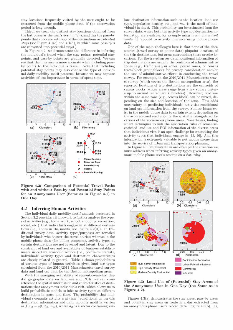
Third, we treat the distinct stay locations obtained fromthe last phase as the user’s destinations, and flag the pass-bypoints that collocate with any of the destinations as potentialstays (see Figure 4.1(c) and 4.1(d), in which some pass-by’sare converted into potential stays ).

In Figure 4.2, we demonstrate the difference in inferringthe individual’s travel when the stay points, potential staypoints, and pass-by points are gradually detected. We cansee that the inference is more accurate when including pass-by points to the individual’s travel. Note that includingpotential stay points may also change the type of individ-ual daily mobility motif patterns, because we may captureactivities of less importance in terms of spent time.

9:57

9:3020:14

14:59

11:52


9:579:30

21:03

14:5911:52

10:55


9:579:30

21:03

20:14

14:59

14:5813:55

11:14

11:13

11:11

11:0811:08

10:5510:23


# Potential Stay

@ Passby

! Observed Stay

!( Phone Records

Potential Routing

20:14

11:52

#

#C

D!

#

#

##

#!

!

#9:30A

B

E

20:14

21:03

10:55

9:57

11:5214:59

A B

C

D

E

(a) (b)

(c) (d)

Figure 4.2: Comparison of Potential Travel Pathswith and without Pass-by and Potential Stay Pointsfor an Anonymous User (Same as in Figure 4.1) inOne Day

4.2 Inferring Human ActivitiesThe individual daily mobility motif analysis presented in

Section 3.2 provides a framework to further analyze the type-s of activities (e.g., home, work, school, shopping, recreation,social, etc.) that individuals engage in at different destina-tions (i.e., nodes in the motifs, see Figure 4.2(d)). In tra-ditional survey data, activity types/purposes are revealedby individuals who answer the travel dairies; whereas in themobile phone data (for billing purposes), activity types atcertain destinations are not revealed and latent. Due to theconstraint of land use and availability of business establish-ments in certain economic sectors (i.e., points-of-interest),individuals’ activity types and destination characteristicsare closely related in general. Table 1 shows probabilitiesof various types of human activities given land use typescalculated from the 2010/2011 Massachusetts travel surveydata and land use data for the Boston metropolitan area.

With the emerging availability of semantic-enriched dig-ital geographic data on land use and POIs, we can crossreference the spatial information and characteristics of desti-nations that anonymous individuals visit, which allows us tobuild probabilistic models to infer activity types at differentdestinations in space and time. The probability that indi-vidual i commits activity a at time t conditional on her/hisdestination information and daily mobility motif is writtenas f(ait = a|t, dit,mid), where dit is a vector containing var-

ious destination information such as the location, land-usetype, population density, etc., and mid is the motif of indi-vidual i in day d. This probability can be estimated from thesurvey data, where both the activity type and destination in-formation are available, for example using multinomial logitmodel [3], applied to activity inference using mobile phonedata.

One of the main challenges here is that none of the datasources (travel survey or phone data) pinpoint locations ofthe trip destinations, but areas surrounding these precise lo-cations. For the travel survey data, locational information oftrip destinations are usually the centroids of administrativezones (e.g., traffic analysis zones, postal zones, or censustract/block group/block) for privacy consideration and/orthe ease of administrative efforts in conducting the travelsurvey. For example, in the 2010/2011 Massachusetts trav-el survey (which covers the Boston metropolitan area), thereported locations of trip destinations are the centroids ofcensus blocks (whose areas range from a few square meter-s up to around ten square kilometers). However, land usewithin the same zone (e.g., census block) can be mixed, de-pending on the size and location of the zone. This addsuncertainty in predicting individuals’ activities conditionalon land use information from the survey. Similar issues ex-ist in the mobile phone data to certain extent, depending onthe accuracy and resolution of the spatially triangulated lo-cations of the anonymous phone users. Nonetheless, findingsmart techniques to link the association rules of semantic-enriched land use and POI information of the diverse areasthat individuals visit is an open challenge for estimating theactivity types that individuals engage in [45, 46]. And thisinformation is extremely valuable to put mobile phone datainto the service of urban and transportation planning.

In Figure 4.3, we illustrate in one example the situation wemust address when inferring activity types given an anony-mous mobile phone user’s records on a Saturday.

10:55

0 0.25 0.5 0.75 1Kilometers

9:57

9:30

21:03

20:14

0 0.4 0.8 1.2 1.6Kilometers

!!

14:5911:52

0 0.2 0.4 0.6 0.8Kilometers

! ! ! ! ! ! ! !

! ! ! ! ! ! ! !

! ! ! ! ! ! ! !

! ! ! ! ! ! ! !

! ! ! ! ! ! ! !

! ! ! ! ! ! ! !

! ! ! ! ! ! ! !

! ! ! ! ! ! ! !

Multi-Family Residential

! ! ! ! ! ! ! ! !

! ! ! ! ! ! ! ! !

! ! ! ! ! ! ! ! !

! ! ! ! ! ! ! ! !

! ! ! ! ! ! ! ! !

High Density Residential

! ! ! !

! ! ! !

! ! ! !

! ! ! ! !

! ! ! ! !

Medium Density Residential

9:57

9:30

21:03

20:14

14:5911:52

10:55


Participation Recreation

Urban Public/Institutional

Commercial

Industrial

03030303

014

03

140

030303

5555

KiKi(a) (b)

(c) (d)

AB

C

D

E

C

D

A

B

E

Figure 4.3: Land Use of (Potential) Stay Areas ofthe Anonymous User in One Day (the Same as inFigure 4.2).

Figures 4.3(a) demonstrates the stay areas, pass-by areasand potential stay areas en route in a day extracted froman anonymous phone user’s record data. Figure 4.3(b), (c),

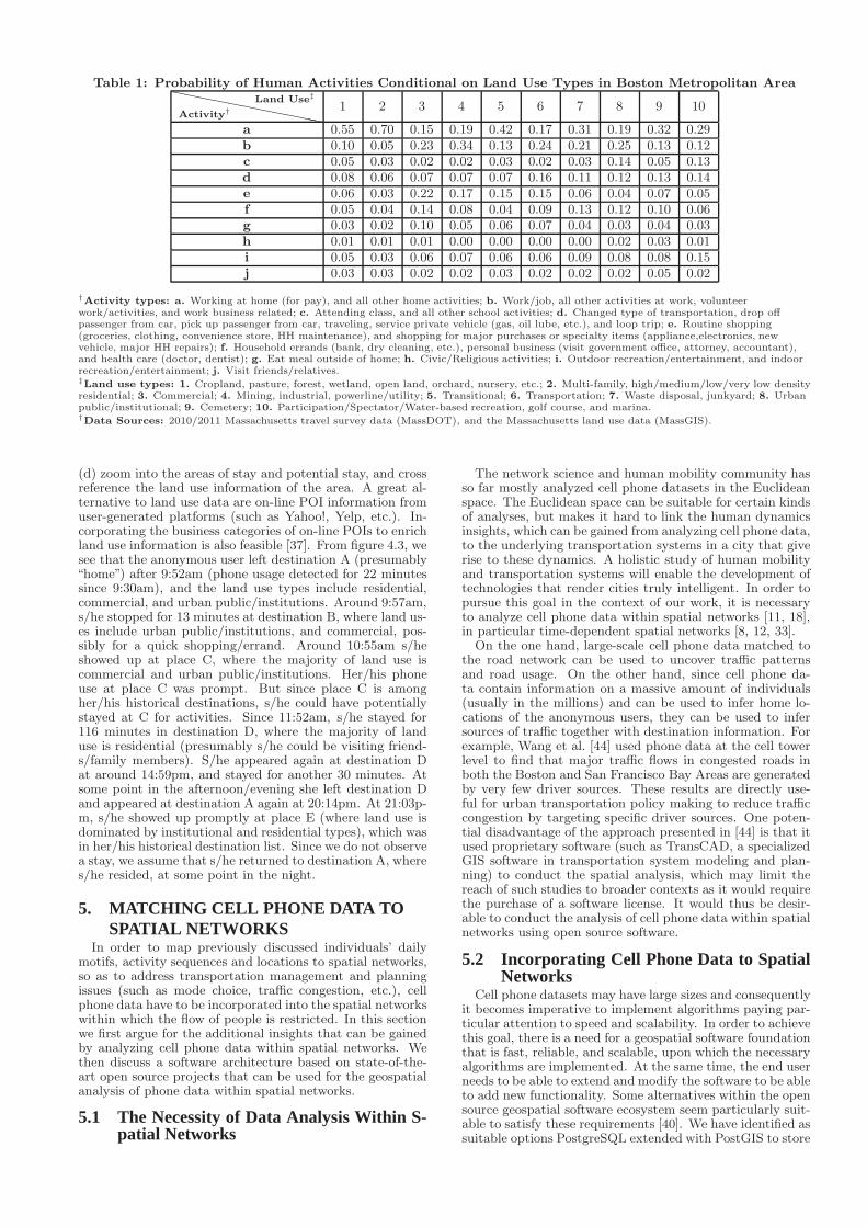
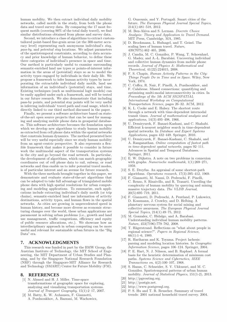
Table 1: Probability of Human Activities Conditional on Land Use Types in Boston Metropolitan Area``````````

Activity†

Land Use‡

1 2 3 4 5 6 7 8 9 10

a 0.55 0.70 0.15 0.19 0.42 0.17 0.31 0.19 0.32 0.29b 0.10 0.05 0.23 0.34 0.13 0.24 0.21 0.25 0.13 0.12c 0.05 0.03 0.02 0.02 0.03 0.02 0.03 0.14 0.05 0.13d 0.08 0.06 0.07 0.07 0.07 0.16 0.11 0.12 0.13 0.14e 0.06 0.03 0.22 0.17 0.15 0.15 0.06 0.04 0.07 0.05f 0.05 0.04 0.14 0.08 0.04 0.09 0.13 0.12 0.10 0.06g 0.03 0.02 0.10 0.05 0.06 0.07 0.04 0.03 0.04 0.03h 0.01 0.01 0.01 0.00 0.00 0.00 0.00 0.02 0.03 0.01i 0.05 0.03 0.06 0.07 0.06 0.06 0.09 0.08 0.08 0.15j 0.03 0.03 0.02 0.02 0.03 0.02 0.02 0.02 0.05 0.02

†Activity types: a. Working at home (for pay), and all other home activities; b. Work/job, all other activities at work, volunteerwork/activities, and work business related; c. Attending class, and all other school activities; d. Changed type of transportation, drop offpassenger from car, pick up passenger from car, traveling, service private vehicle (gas, oil lube, etc.), and loop trip; e. Routine shopping(groceries, clothing, convenience store, HH maintenance), and shopping for major purchases or specialty items (appliance,electronics, newvehicle, major HH repairs); f. Household errands (bank, dry cleaning, etc.), personal business (visit government office, attorney, accountant),and health care (doctor, dentist); g. Eat meal outside of home; h. Civic/Religious activities; i. Outdoor recreation/entertainment, and indoorrecreation/entertainment; j. Visit friends/relatives.‡Land use types: 1. Cropland, pasture, forest, wetland, open land, orchard, nursery, etc.; 2. Multi-family, high/medium/low/very low densityresidential; 3. Commercial; 4. Mining, industrial, powerline/utility; 5. Transitional; 6. Transportation; 7. Waste disposal, junkyard; 8. Urbanpublic/institutional; 9. Cemetery; 10. Participation/Spectator/Water-based recreation, golf course, and marina.†Data Sources: 2010/2011 Massachusetts travel survey data (MassDOT), and the Massachusetts land use data (MassGIS).

(d) zoom into the areas of stay and potential stay, and crossreference the land use information of the area. A great al-ternative to land use data are on-line POI information fromuser-generated platforms (such as Yahoo!, Yelp, etc.). In-corporating the business categories of on-line POIs to enrichland use information is also feasible [37]. From figure 4.3, wesee that the anonymous user left destination A (presumably“home”) after 9:52am (phone usage detected for 22 minutessince 9:30am), and the land use types include residential,commercial, and urban public/institutions. Around 9:57am,s/he stopped for 13 minutes at destination B, where land us-es include urban public/institutions, and commercial, pos-sibly for a quick shopping/errand. Around 10:55am s/heshowed up at place C, where the majority of land use iscommercial and urban public/institutions. Her/his phoneuse at place C was prompt. But since place C is amongher/his historical destinations, s/he could have potentiallystayed at C for activities. Since 11:52am, s/he stayed for116 minutes in destination D, where the majority of landuse is residential (presumably s/he could be visiting friend-s/family members). S/he appeared again at destination Dat around 14:59pm, and stayed for another 30 minutes. Atsome point in the afternoon/evening she left destination Dand appeared at destination A again at 20:14pm. At 21:03p-m, s/he showed up promptly at place E (where land use isdominated by institutional and residential types), which wasin her/his historical destination list. Since we do not observea stay, we assume that s/he returned to destination A, wheres/he resided, at some point in the night.

5. MATCHING CELL PHONE DATA TOSPATIAL NETWORKS

In order to map previously discussed individuals’ dailymotifs, activity sequences and locations to spatial networks,so as to address transportation management and planningissues (such as mode choice, traffic congestion, etc.), cellphone data have to be incorporated into the spatial networkswithin which the flow of people is restricted. In this sectionwe first argue for the additional insights that can be gainedby analyzing cell phone data within spatial networks. Wethen discuss a software architecture based on state-of-the-art open source projects that can be used for the geospatialanalysis of phone data within spatial networks.

5.1 The Necessity of Data Analysis Within S-patial Networks

The network science and human mobility community hasso far mostly analyzed cell phone datasets in the Euclideanspace. The Euclidean space can be suitable for certain kindsof analyses, but makes it hard to link the human dynamicsinsights, which can be gained from analyzing cell phone data,to the underlying transportation systems in a city that giverise to these dynamics. A holistic study of human mobilityand transportation systems will enable the development oftechnologies that render cities truly intelligent. In order topursue this goal in the context of our work, it is necessaryto analyze cell phone data within spatial networks [11, 18],in particular time-dependent spatial networks [8, 12, 33].

On the one hand, large-scale cell phone data matched tothe road network can be used to uncover traffic patternsand road usage. On the other hand, since cell phone da-ta contain information on a massive amount of individuals(usually in the millions) and can be used to infer home lo-cations of the anonymous users, they can be used to infersources of traffic together with destination information. Forexample, Wang et al. [44] used phone data at the cell towerlevel to find that major traffic flows in congested roads inboth the Boston and San Francisco Bay Areas are generatedby very few driver sources. These results are directly use-ful for urban transportation policy making to reduce trafficcongestion by targeting specific driver sources. One poten-tial disadvantage of the approach presented in [44] is that itused proprietary software (such as TransCAD, a specializedGIS software in transportation system modeling and plan-ning) to conduct the spatial analysis, which may limit thereach of such studies to broader contexts as it would requirethe purchase of a software license. It would thus be desir-able to conduct the analysis of cell phone data within spatialnetworks using open source software.

5.2 Incorporating Cell Phone Data to SpatialNetworks

Cell phone datasets may have large sizes and consequentlyit becomes imperative to implement algorithms paying par-ticular attention to speed and scalability. In order to achievethis goal, there is a need for a geospatial software foundationthat is fast, reliable, and scalable, upon which the necessaryalgorithms are implemented. At the same time, the end userneeds to be able to extend and modify the software to be ableto add new functionality. Some alternatives within the opensource geospatial software ecosystem seem particularly suit-able to satisfy these requirements [40]. We have identified assuitable options PostgreSQL extended with PostGIS to store

and manipulate the cell phone data and the spatial network-s, and pgRouting to add geospatial routing capabilities tothe database. Beyond the availability of numerous featuresthat make it possible to conduct various analyses, these opensource tools provide a great foundation upon which to im-plement extensions related to time dependency [34, 10, 9]and multimodality [7] for example.

PostgreSQL is a powerful, open source object-relationaldatabase system [22]. It is fully ACID compliant, has fullsupport for foreign keys, joins, views, triggers, and storedprocedures. It includes most SQL:2008 data types and alsosupports storage of binary large objects, including pictures,sounds, or video. It has native programming interfaces forPython, which is our programming language of choice foralgorithm implementation and analysis. It is highly scalablein terms of the quantity of data it can manage, with an un-limited maximum database size and a 32 TB maximum tablesize. The key component that makes PostgreSQL suitablefor geospatial analysis is PostGIS.

PostGIS is a spatial database extender for PostgreSQLthat adds support for geographic objects, allowing Post-greSQL to be used as a spatial database for geographic in-formation systems (GIS) [21]. PostGIS adds support for ge-ographic objects allowing location queries to be run in SQL.It adds extra types (geometry, geography, raster and other-s) as well as functions, operators, and index enhancementsthat apply to these spatial types. This PostgreSQL/PostGIScombination results in a fast, feature-rich, and robust spa-tial database management system. Navigation for road net-works requires complex routing algorithms that support turnrestrictions and ideally time-dependent attributes. Toward-s this end, geospatial routing can be done at the databaselevel with pgRouting.

pgRouting is a library that extends PostgreSQL/PostGISto support geospatial routing and adds routing functional-ity to the database [20]. It provides a variety of tools forshortest path search, including functions for Shortest PathDikstra, Shortest Path A-Star, Shortest Path Shooting-Star(routing with turn restrictions), Traveling Salesman Prob-lem (TSP), and Driving Distance calculation. The key valueof pgRouting is that it allows these high-level functions torun at the database level. Furthermore, the database rout-ing approach has two main advantages that make it suitablefor eventually incorporating time-dependency into the prob-lem. First, any data changes in the database will be takeninto account instantaneously by the routing engine. Second,the “cost” parameter can be dynamically calculated throughSQL and its value come from multiple fields or tables.

PostgresSQL/PostGIS are very useful not only to perfor-m routing queries through pgRouting, but also—togetherwith the python interface capabilities—to manage the rawdata (after some initial data filtering and processing) and tohandle the rest of the algorithms for converting the raw da-ta into manageable individuals’ daily traces, activities, andtrip destinations, etc. More specifically, the raw cell phonedata and the corresponding local road network can be storedin a PostgreSQL/PostGIS database. pgRouting can then beused to perform geospatial routing and enable the executionof analyses related to road usage as in [44] but based on anopen source software architecture. The different algorithmsto process the data as have been presented in the paper canbe implemented in Python and use the open-source Pythonmodule PyGreSQL to interface to the PostgreSQL database.As the data gets refined, the smaller subsets can be storedin new tables and data processing can proceed from thesesubsets.

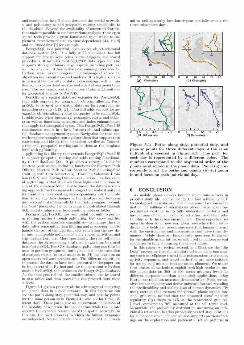
Figure 5.1 gives a preview of the advantages of analyzingcell phone data in a road network. In this figure we cansee the paths along stay, potential stay, and pass-by pointsfor the same person as in Figures 4.1 and 4.2 for three dif-ferent days. These paths give an approximate indication ofthe mobility of a person throughout time while taking intoaccount the dynamic constraints of the spatial networks (inthis case the road network) to which the human dynamicsare subjected. Notice how the home location of the individ-

ual as well as nearby locations repeat spatially among thethree subsequent days.

0 10 20 30 40 50Kilometers

0 8 16 24 32 40Kilometers

0 4 8KM

0 4 8KM

0 1.5 3 4.5 6 7.5Kilometers

0 0.5 1KM

0 4 8 12 16 20Kilometers

0 1.5 3KM

(a) (b)

(c) (d)

Figure 5.1: Paths along stay, potential stay, andpass-by points for three different days of the sameindividual presented in Figure 4.1. The path foreach day is represented by a different color. Thenumbers correspond to the sequential order of thepoints as observed in the phone data. Panel (a) cor-responds to all the paths and panels (b)–(c) zoomin and focus on each individual day.

6. CONCLUSIONAs mobile phone devices become ubiquitous sensors in

people’s daily life, companied by the fast advancing ICTtechnologies that make available fine-grained location infor-mation for millions of anonymous phone users, great op-portunities exist for us to fully understand patterns andmechanisms of human mobility, activities, and their rela-tionship with the urban environment. These opportunitiesopen the door to an new era, when researchers from inter-disciplinary fields can re-examine ways that human interactwith the environment and mechanisms that drive these dy-namics. While these are fundamental questions to answerfor sustainable urban future, we still need to address severalchallenges in fully embracing the opportunities.

In this paper, we review, extend, and illustrate the “BigData” processing that can translate voluminous urban sens-ing (such as cellphone traces) into parsimonious trip chains,activity sequences, and travel paths that are more suitablefor use by land use and transportation planners. We utilizethree classes of methods to exploit such high-resolution mo-bile phone data (at 200- to 300- meter accuracy level) fordifferent purposes in urban computing applications, usingBoston metropolitan area as a demonstration. First, we an-alyze human mobility and derive universal features revealingthe predictability and scaling laws of human dynamics. Byusing method that extracts individuals’ phone signals intosmall grid cells, we find that the measured users’ mobilityregularity R(t) drops to 64% at the represented grid cel-l level compared to 70% measured at the cell tower level.Meanwhile, the probability distribution measuring an indi-vidual’s returns to her/his previously visited stay locationsfor all phone users in our sample also supports previous find-ings on the exploration and preferential return patterns in

human mobility. We then extract individual daily mobilitynetworks, called motifs in the study, from both the phonedata and travel survey data. By comparing the 17 most fre-quent motifs (covering 90% of the total daily travel), we findsimilar distributions obtained from phone and survey data.

Second, we introduce a class of algorithms to extract custom-tailored point-based fine-grain areas (at the 300-meter accu-racy level) representing each anonymous individual’s stay,pass-by, and potential stay locations. We adjust parametersof the spatiotemporal constraints, according to data accura-cy and prior knowledge of human behavior, to define thesethree categories of individual’s presence in space and time.Our method is particularly useful to examine surroundingsemantic-enriched land use types or points-of-interest infor-mation in the areas of (potential) stays so as to model theactivity types engaged by individuals in their daily life. Wepropose a framework to infer human activity types by incor-porating the extractable individual daily motifs, land useinformation of an individual’s (potential) stays, and time.Existing techniques (such as multinomial logit models) canbe easily applied under such a framework, and will be testedin our future research. We also demonstrate that includingpass-by points, and potential stay points will be very usefulin inferring individuals’ travel path and road usage, which isdirectly linked to our third method discussed in the paper.

Finally, we present a software architecture based on state-of-the-art open source projects that can be used for manag-ing and analyzing mobile phone data in geospatial databas-es. This software architecture becomes the foundation uponwhich we develop new algorithms to study human mobilityas extracted from cell phone data within the spatial networksthat constrain human dynamics. The method presented herewill be very useful especially since we study human mobilityfrom an agent-centric perspective. It also represents a flex-ible framework that makes it possible to consider in futurework the multimodal aspect of the transportation systemsin the city and go beyond the road network. In particular,the development of algorithms, which can match geographiccoordinates out of cell phone data to rail, subway, or roadnetworks and thus enable us to infer potential travel modes,is of particular interest and an avenue for future research.

With the three methods brought together in this paper, wedemonstrate and evaluate state-of-the-art algorithms thatcan be adopted to take full advantage of triangulated mobilephone data with high spatial resolutions for urban comput-ing and modeling applications. To summarize, such appli-cations include extracting individual’s daily motifs (or tripchains), semantic-enriched land use information of activitydestinations, activity types, and human flows in the spatialnetworks. As cities are growing in unprecedented speed inhuman history, and become more diverse as economic struc-turing changes over the world, these urban applications areparamount in solving urban problems (i.e., growth and landuse management, traffic congestions, efficiency and equityof public resource allocations, etc.). We showcase how aninterdisciplinary approach in urban computing can be moreuseful and relevant for sustainable urban futures in the “BigData” era.

7. ACKNOWLEDGMENTSThis research was funded in part by the BMW Group, the

Austrian Institute of Technology, the MIT School of Engi-neering, the MIT Department of Urban Studies and Plan-ning, and by the Singapore National Research Foundation(NRF) through the Singapore-MIT Alliance for Researchand Technology (SMART) Center for Future Mobility (FM).

8. REFERENCES[1] N. Ahmed and H. J. Miller. Time-space

transformations of geographic space for exploring,analyzing and visualizing transportation systems.Journal of Transport Geography, 15(1):2–17, 2007.

[2] M. Batty, K. W. Axhausen, F. Giannotti,A. Pozdnoukhov, A. Bazzani, M. Wachowicz,

G. Ouzounis, and Y. Portugali. Smart cities of thefuture. The European Physical Journal Special Topics,214(1):481–518, 2012.

[3] M. Ben-Akiva and S. Lerman. Discrete ChoiceAnalysis: Theory and Application to Travel Demand.MIT Press, Cambridge, MA, 1985.

[4] D. Brockmann, L. Hufnagel, and T. Geisel. Thescaling laws of human travel. Nature,439(7075):462–465, 2006.

[5] J. Candia, M. C. Gonzalez, P. Wang, T. Schoenharl,G. Madey, and A.-L. Barabasi. Uncovering individualand collective human dynamics from mobile phonerecords. Journal of Physics A: Mathematical andTheoretical, 41(22):224015, 2008.

[6] F. S. Chapin. Human Activity Patterns in the City:Things People Do in Time and in Space. Wiley, NewYork, 1974.

[7] C. Coffey, R. Nair, F. Pinelli, A. Pozdnoukhov, andF. Calabrese. Missed connections: quantifying andoptimizing multi-modal interconnectivity in cities. InProceedings of the 5th ACM SIGSPATIALInternational Workshop on ComputationalTransportation Science, pages 26–32. ACM, 2012.

[8] K. L. Cooke and E. Halsey. The shortest routethrough a network with time-dependent internodaltransit times. Journal of mathematical analysis andapplications, 14(3):493–498, 1966.

[9] U. Demiryurek, F. Banaei-Kashani, and C. Shahabi.Efficient k-nearest neighbor search in time-dependentspatial networks. In Database and Expert SystemsApplications, pages 432–449. Springer, 2010.

[10] U. Demiryurek, F. Banaei-Kashani, C. Shahabi, andA. Ranganathan. Online computation of fastest pathin time-dependent spatial networks, pages 92–111.Advances in Spatial and Temporal Databases.Springer, 2011.

[11] E. W. Dijkstra. A note on two problems in connexionwith graphs. Numerische mathematik, 1(1):269–271,1959.

[12] S. E. Dreyfus. An appraisal of some shortest-pathalgorithms. Operations research, 17(3):395–412, 1969.

[13] F. Giannotti, M. Nanni, D. Pedreschi, F. Pinelli,C. Renso, S. Rinzivillo, and R. Trasarti. Unveiling thecomplexity of human mobility by querying and miningmassive trajectory data. The VLDB Journal,20(5):695–719, 2011.

[14] F. Giannotti, D. Pedreschi, A. Pentland, P. Lukowicz,D. Kossmann, J. Crowley, and D. Helbing. Aplanetary nervous system for social mining andcollective awareness. The European Physical JournalSpecial Topics, 214(1):49–75, 2012.

[15] M. Gonzalez, C. Hidalgo, and A. Barabasi.Understanding individual human mobility patterns.Nature, 453(7196):779–782, 2008.

[16] T. Hagerstrand. Reflections on ”what about people inregional science?”. Papers in Regional Science,66(1):1–6, 1989.

[17] R. Hariharan and K. Toyama. Project lachesis:parsing and modeling location histories. In GeographicInformation Science, pages 106–124. Springer, 2004.

[18] P. E. Hart, N. J. Nilsson, and B. Raphael. A formalbasis for the heuristic determination of minimum costpaths. Systems Science and Cybernetics, IEEETransactions on, 4(2):100–107, 1968.

[19] S. Hasan, C. Schneider, S. V. Ukkusuri, and M. C.Gonzalez. Spatiotemporal patterns of urban humanmobility. Journal of Statistical Physics, 151(1-2), 2013.

[20] http://pgrouting.org.[21] http://postgis.net.[22] http://www.postgresql.org.[23] P. S. Hu and T. R. Reuscher. Summary of travel

trends: 2001 national household travel survey. 2004.

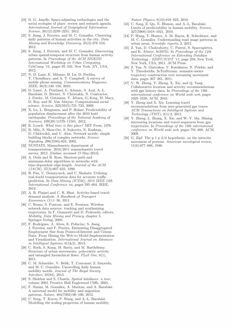
[24] D. G. Janelle. Space-adjusting technologies and thesocial ecologies of place: review and research agenda.International Journal of Geographical InformationScience, 26(12):2239–2251, 2012.

[25] S. Jiang, J. Ferreira, and M. C. Gonzalez. Clusteringdaily patterns of human activities in the city. DataMining and Knowledge Discovery, 25(3):478–510,2012.

[26] S. Jiang, J. Ferreira, and M. C. Gonzalez. Discoveringurban spatial-temporal structure from human activitypatterns. In Proceedings of the ACM SIGKDDInternational Workshop on Urban Computing,UrbComp ’12, pages 95–102, New York, NY, USA,2012.

[27] N. D. Lane, E. Miluzzo, H. Lu, D. Peebles,T. Choudhury, and A. T. Campbell. A survey ofmobile phone sensing. Communications Magazine,IEEE, 48(9):140–150, 2010.

[28] D. Lazer, A. Pentland, L. Adamic, S. Aral, A.-L.Barabasi, D. Brewer, N. Christakis, N. Contractor,J. Fowler, M. Gutmann, T. Jebara, G. King, M. Macy,D. Roy, and M. Van Alstyne. Computational socialscience. Science, 323(5915):721–723, 2009.

[29] X. Lu, L. Bengtsson, and P. Holme. Predictability ofpopulation displacement after the 2010 haitiearthquake. Proceedings of the National Academy ofSciences, 109(29):11576–11581, 2012.

[30] K. Lynch. What time is this place? MIT Press, 1976.[31] R. Milo, S. Shen-Orr, S. Itzkovitz, N. Kashtan,

D. Chklovskii, and U. Alon. Network motifs: simplebuilding blocks of complex networks. ScienceSignaling, 298(5594):824, 2002.

[32] NUSTATS. Massachusetts department oftransportation: 2010/2011 massachusetts travelsurvey. 2012. [Online; accessed 17-May-2013].

[33] A. Orda and R. Rom. Shortest-path andminimum-delay algorithms in networks withtime-dependent edge-length. Journal of the ACM(JACM), 37(3):607–625, 1990.

[34] B. Pan, U. Demiryurek, and C. Shahabi. Utilizingreal-world transportation data for accurate trafficprediction. In Data Mining (ICDM), 2012 IEEE 12thInternational Conference on, pages 595–604. IEEE,2012.

[35] A. R. Pinjari and C. R. Bhat. Activity-based traveldemand analysis. A Handbook of TransportEconomics, (1):1–36, 2011.

[36] C. Renso, S. Puntoni, and E. Frentzos. Wirelessnetwork data sources: tracking and synthesizingtrajectories. In F. Giannotti and D. Pedreschi, editors,Mobility, Data Mining and Privacy, chapter 3.Springer-Verlag, 2008.

[37] F. Rodrigues, A. Alves, E. Polisciuc, S. Jiang,J. Ferreira, and F. Pereira. Estimating DisaggregatedEmployment Size from Points-of-Interest and CensusData: From Mining the Web to Model Implementationand Visualization. International Journal on Advancesin Intelligent Systems, 6(1&2), 2013.

[38] C. Roth, S. Kang, M. Batty, and M. Barthelemy.Structure of urban movements: polycentric activityand entangled hierarchical flows. PLoS One, 6(1),2011.

[39] C. M. Schneider, V. Belik, T. Couronne, Z. Smoreda,and M. C. Gonzalez. Unravelling daily humanmobility motifs. Journal of The Royal SocietyInterface, 10(84), 2013.

[40] S. Shekhar and S. Chawla. Spatial databases: a tour,volume 2003. Prentice Hall Englewood Cliffs, 2003.

[41] F. Simini, M. Gonzalez, A. Maritan, and A. Barabasi.A universal model for mobility and migrationpatterns. Nature, 484(7392):96–100, 2012.

[42] C. Song, T. Koren, P. Wang, and A.-L. Barabasi.Modelling the scaling properties of human mobility.

Nature Physics, 6(10):818–823, 2010.[43] C. Song, Z. Qu, N. Blumm, and A.-L. Barabasi.

Limits of predictability in human mobility. Science,327(5968):1018–1021, 2010.

[44] P. Wang, T. Hunter, A. M. Bayen, K. Schechtner, andM. C. Gonzalez. Understanding road usage patterns inurban areas. Scientific reports, 2, 2012.

[45] Z. Yan, D. Chakraborty, C. Parent, S. Spaccapietra,and K. Aberer. SeMiTri. In Proceedings of the 14thInternational Conference on Extending DatabaseTechnology - EDBT/ICDT ’11, page 259, New York,New York, USA, 2011. ACM Press.

[46] Z. Yan, N. Giatrakos, V. Katsikaros, N. Pelekis, andY. Theodoridis. SeTraStream: semantic-awaretrajectory construction over streaming movementdata. pages 367–385, 2011.

[47] V. W. Zheng, Y. Zheng, X. Xie, and Q. Yang.Collaborative location and activity recommendationswith gps history data. In Proceedings of the 19thinternational conference on World wide web, pages1029–1038. ACM, 2010.

[48] Y. Zheng and X. Xie. Learning travelrecommendations from user-generated gps traces.ACM Transactions on Intelligent Systems andTechnology (TIST), 2(1):2, 2011.

[49] Y. Zheng, L. Zhang, X. Xie, and W.-Y. Ma. Mininginteresting locations and travel sequences from gpstrajectories. In Proceedings of the 18th internationalconference on World wide web, pages 791–800. ACM,2009.

[50] G. Zipf. The p 1 p 2/d hypothesis: on the intercitymovement of persons. American sociological review,11(6):677–686, 1946.

A Review of Urban Computing for Mobile Phone Traces ...ares.lids.mit.edu/fm/documents/review.pdfA...

Documents

Transcript of A Review of Urban Computing for Mobile Phone Traces ...ares.lids.mit.edu/fm/documents/review.pdfA...