Approximating the Performance of a Last Mile...

1

Approximating the Performance of a “Last Mile” Transportation System

Hai Wang and Amedeo Odoni

Massachusetts Institute of Technology Abstract: The Last Mile Problem (LMP) refers to the provision of travel service from the nearest public transportation node to a home or office. We study the supply side of this problem in a stochastic setting, with batch demands resulting from the arrival of groups of passengers at rail stations or bus stops who request last-mile service. Closed-form bounds and approximations are derived for the performance of Last Mile Transportations Systems as a function of the fundamental design parameters of such systems. An initial set of results is obtained for the case in which a fleet of vehicles of unit capacity provides the Last Mile service and each delivery route consists of a simple round-trip between the rail station and bus stop and the single passenger’s destination. These results are then extended to the general case in which the capacity of a vehicle is an arbitrary, but typically small (under 10) number. It is shown through comparisons with simulation results, that a particular strict upper bound and an approximate upper bound, both derived under similar assumptions, perform consistently and remarkably well for the entire spectrum of input values and conditions simulated. These expressions can therefore be used for the preliminary planning and design of Last Mile Transportation Systems, especially for determining approximately resource requirements, such as the number of vehicles/servers needed to achieve some pre-specified level of service.

Keywords: Last mile problem; queuing; batch demands; waiting time bounds; cyclic assignment.

1. Introduction and Literature Survey

The Last Mile Problem (LMP) refers to the provision of travel service from home or workplace to the nearest public transportation node (“first mile”) or vice versa (“last mile”). This public transportation node could be the nearest rapid transit rail station or a stop of a scheduled bus line. The unavailability of this type of service is one of the main deterrents to the use of public transport in urban areas, especially for certain demographic groups, such as schoolchildren, seniors and the disabled. Currently, the default solutions to the LMP are walking, taking a taxi, or driving a private vehicle.

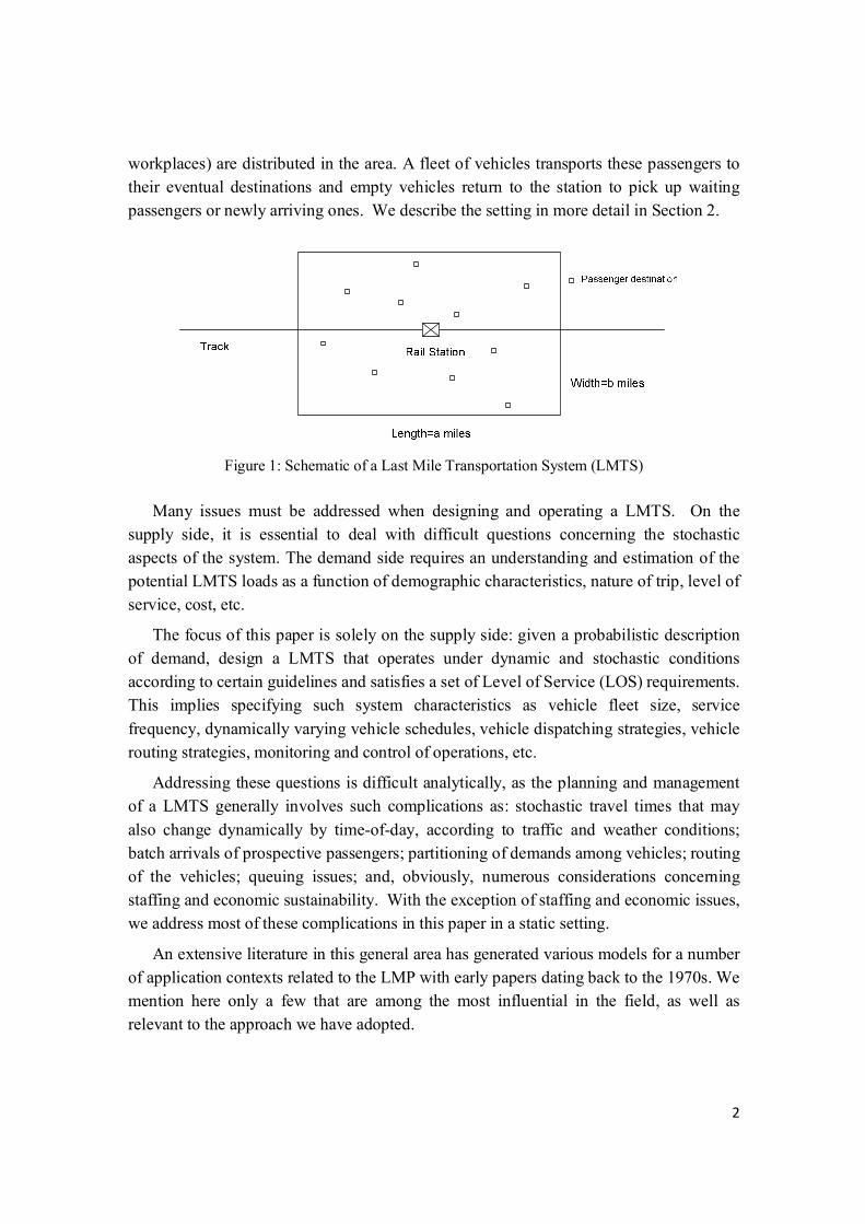
A conceptual Last Mile Transportation System (LMTS) is described schematically in Figure 1, which shows an urban area surrounding a public-transit rail station, where trains arrive and discharge passengers. The passengers’ final destinations (homes, offices and

2

workplaces) are distributed in the area. A fleet of vehicles transports these passengers to their eventual destinations and empty vehicles return to the station to pick up waiting passengers or newly arriving ones. We describe the setting in more detail in Section 2.

Figure 1: Schematic of a Last Mile Transportation System (LMTS)

Many issues must be addressed when designing and operating a LMTS. On the

supply side, it is essential to deal with difficult questions concerning the stochastic aspects of the system. The demand side requires an understanding and estimation of the potential LMTS loads as a function of demographic characteristics, nature of trip, level of service, cost, etc.

The focus of this paper is solely on the supply side: given a probabilistic description of demand, design a LMTS that operates under dynamic and stochastic conditions according to certain guidelines and satisfies a set of Level of Service (LOS) requirements. This implies specifying such system characteristics as vehicle fleet size, service frequency, dynamically varying vehicle schedules, vehicle dispatching strategies, vehicle routing strategies, monitoring and control of operations, etc.

Addressing these questions is difficult analytically, as the planning and management of a LMTS generally involves such complications as: stochastic travel times that may also change dynamically by time-of-day, according to traffic and weather conditions; batch arrivals of prospective passengers; partitioning of demands among vehicles; routing of the vehicles; queuing issues; and, obviously, numerous considerations concerning staffing and economic sustainability. With the exception of staffing and economic issues, we address most of these complications in this paper in a static setting.

An extensive literature in this general area has generated various models for a number of application contexts related to the LMP with early papers dating back to the 1970s. We mention here only a few that are among the most influential in the field, as well as relevant to the approach we have adopted.

3

The Dynamic Traveling Repairman Problem (DTRP) was introduced in two papers by Bertsimas and Van Ryzin. They consider the DTRP in the cases of a single-vehicle “fleet” [1] and of multiple vehicles [2]. The Dynamic Pick-up and Delivery Problem (DPDP) was studied by Swihart and Papastavrou [3], who derived bounds on the performance of several DPDP variants for light and heavy traffic. The Car Pooling Problem (CPP), introduced by Baldacci, Maniezzo and Mingozzi [4] also has features similar to the LMP – or, more exactly, to the First Mile Problem. This paper presents both exact and heuristic methods for solving the CPP based on integer programming formulations. Finally, a large number of papers have dealt with the Dial-a-Ride Problem (DARP) – see, e.g., Jaw, Odoni, Psaraftis and Wilson [15]. A fine critical review of the DARP literature by Cordeau and Laporte [5] underlines, among other points, the fact that this body of work does not address well some of the queuing aspects of the subject systems – a deficiency that this paper tries to remedy.

It should also be noted that similarities exist between the LMP and various queuing, dispatching, routing, and resource allocation problems arising in entirely different contexts such as the design of manufacturing systems, the operation of elevator banks, and the scheduling of school-bus systems.

The major difference between the LMP and the more “traditional” problems identified above is that, in the LMP, passengers arrive in (possibly large) batches, not singly. Moreover, the size of these batches is a random variable. Queuing systems with batch arrivals are notoriously difficult analytically. A further complication is that the “service times” of passengers are determined by the length (or the duration) of the routes traveled by the fleet of delivery vehicles. Thus, in designing a LMTS, it is necessary to consider simultaneously the problems of: allocating passengers among vehicles; routing the vehicles and estimating the lengths of the routes; and computing the queuing performance characteristics of the system.

The main body of this paper is organized as follows. In Section 2, we describe in more detail the version of the LMP problem that we are studying and discuss the associated fundamental assumptions. It will be seen that the problem analyzed is quite generic and that by relaxing one or more of the assumptions, one can capture a broad range of interesting variations. Section 3 then outlines the overall approach utilized to derive our results: we begin by deriving a set of queuing results by considering a fleet of vehicles with capacity for a single passenger ( = 1) and then extend the analysis by allowing the vehicle capacity to be arbitrary and by incorporating the resulting travel time estimates into the queuing expressions derived for the = 1 case. Section 4, presents our analysis and results for the single-capacity case. We derive three different approximate expressions for queuing performance as a function of the design parameters of the LMTS and then identify, through a set of simulation experiments, the expression that performs

4

best – and, in fact, approximates very well the observed waiting times. Section 5 first derives approximate analytical expressions for the travel times associated with fleets consisting of vehicles with a capacity of up to 20 passengers and then applies the queuing approximation derived in Section 4 to the multi-passenger capacity case. The results again compare well with those obtained from a simulation. Sections 4 and 5 contain only outlines of the lengthy derivations of our results. A sequence of technical Appendices provides the details. Finally, Section 10 contains a summary and concluding remarks.

2. Problem Description and Assumptions

We now describe in more detail the LMP scenario of Figure 1. The Last Mile Transportation System (LMTS) would operate as follows: Let STA be the transit rail station served by the LMTS and consider a passenger, PAX, who will board a train at station ORIGIN for the purpose of traveling to STA and will then board a LMTS vehicle for transport to her home. PAX will be required to provide advance notice to LMTS of her impending arrival at STA. The time interval between the advance notice and the actual arrival of PAX at STA will be of the order of several minutes (e.g., at least 5 or 10 minutes) to give the LMTS system sufficient time to plan the service of PAX. In practical terms, the advance notice could be generated by PAX in a number of alternative ways. For example, PAX could use a smart-phone when she arrives at ORIGIN or when she enters her train to STA; or, she could tap a smart card on a special-purpose screen, as she is entering ORIGIN or while aboard the train. The resulting message to the LMTS will include the expected time of arrival of PAX at STA (easy to predict, once the passenger is at the ORIGIN station or aboard a train) and her ultimate destination, e.g., her home address. (If the great majority of LMTS users will be subscribers whose home addresses will be pre-registered on a file, then the only information that PAX would have to provide will be an identification number.)

Once the information about PAX is received the LMTS will assign PAX to one of the vehicles of the LMTS fleet, plan the route of that vehicle so it includes a visit to the ultimate destination of PAX, estimate the departure time of the vehicle from STA, and notify PAX accordingly. PAX will receive a message (on her smart-phone or by tapping her card on a screen when she arrives at STA) that indicates the vehicle she has been assigned to and the planned departure time of the vehicle from STA (e.g., “please board Vehicle 123 which will depart from STA at 4:26 PM”). Once all the passengers assigned to a vehicle are on board, the vehicle will execute a delivery route, visiting the destination of each of the passengers and will then return to STA to pick up the passengers for its next delivery tour.

5

The LMTS described above may be difficult to implement due to many practical issues and considerations. However, we have chosen to study it because it possesses the generic system features that we are most interested in: arrivals of passengers in “batches” (groups) at STA; “real-time” clustering of passengers for assignment to a fleet of vehicles; “real-time” routing of the vehicles to deliver the passengers on board; and fast computation of waiting times and other performance parameters so that, for example, passengers can be notified in a timely way of the departure time of the vehicle they have been assigned to/ informed of the expected departure times and intended use of the LMTS. Actual implementations would involve some simpler variants of the above features.

Given the service region geometry, passenger demand rates, the spatial distribution of the passenger destinations, and the number, capacity and travel speed of the LMTS vehicles, examples of performance metrics that we eventually wish to compute include: the average waiting time until boarding a delivery vehicle, the average riding time of passengers, the average waiting time until delivery, the minimum number of vehicles we need to reach stable operation, vehicle productivity and workload, and eventually (but not in this paper) the general cost of operating the system and various service vs. cost trade-offs.

We now identify briefly the specifics of the model considered. With reference to Figure 1, we make the following assumptions: (i) headways, h, between arrivals of trains at the station (and discharges of passengers) are constant; (ii) passengers are discharged in batches after each train’s arrival; (iii) the batch size is a general random variable, , with known expected value, ( ) = , and variance, ( ) = ; (iv) all passengers arriving in a single batch request service essentially simultaneously; (v) given the size of any particular batch, = , the destinations of the passengers in the batch are distributed in a service region according to a homogeneous spatial Poisson process with parameter ; (vi) the service region is convex and compact with known dimensions; (vii) the delivery fleet (or pick-up fleet, in the case of “First Mile” service) consists of m vehicles, each with integer capacity, c.

We believe that (i) – (vii) are adequately general assumptions for approximating, to a first order, the characteristics of many potential variations of LMTS. Note that our model includes the most difficult, from the analytical point of view, features that one might encounter in an LMTS: batch arrivals, stochastic demand, stochastic service times, and the presence of queuing phenomena interfaced with routing problems.

To ensure that the mathematical expressions presented in Sections 4 and 5 below are adequately concise, we have also used the following three simplifying assumptions: (viii) the service area, where the destinations of the passengers are located, is a × square,

6

with the train station, STA, located at the square’s center; (ix) the travel medium is continuous, homogeneous, and planar; and (x) the travel speed is constant throughout the service region and equal to 1. We have studied a number of variants of assumptions (viii) and (ix), such as cases in which the region is not a square, or the travel metric is Euclidean or rectangular (“right-angle) or contains discontinuities (e.g., barriers to travel), and shown that such mild changes in the assumptions pose no particular challenges.

3. Description of Overall Approach

Sections 4 and 5 of the paper describe in detail our analysis and results. In this section we provide a brief description of the overall approach we have followed to provide perspective for these detailed sections. We have adopted a perspective under which the LMTS is regarded as a spatially distributed queuing system in which the demands are as described in Section 2 (batch arrivals of passengers with a constant headway between the arrivals of successive batches). In line, with typical queuing terminology, we shall refer henceforth to passengers as “customers” of the spatially distributed queuing system. The m parallel servers (the vehicle fleet) serve customers in groups of c or smaller, where c is the capacity of each vehicle. The service time for each group is equal to the travel time associated with a vehicle tour that begins at the station/depot, visits each of the c (or fewer) customer destinations and returns to the station/depot to pick up a new group.

Figure 2 Customer destinations and vehicles routes of the Unit-Capacity, Multi-Vehicle LMP

Because queuing systems with batch arrivals (like the arrivals of passengers at STA)

are notoriously difficult to analyze, we resort to a two-step approach. In Step 1, we assume that = 1, i.e., that the delivery vehicles have unit capacity. Thus, in this case, service times consist simply of the duration of a round-trip between STA and one

7

passenger’s destination (see Figure 2), with the destination being randomly and uniformly distributed within the service area per our assumption (v) in Section 2. In this way we obtain a / / /∞ system in queuing theory notation, where: indicates batch arrivals at constant (“Deterministic”) intervals with the number of arriving passengers in each batch described by random variable ; G denotes the fact that the distribution of service times (i.e., the duration of the round trips between STA and customer destinations) is “general”; and and ∞ indicate, respectively, the number of service vehicles and the fact that no a priori limit is placed on the number of customers waiting for pickup at STA.

As no closed-form expressions are available for the fundamental quantities the performance of a / / /∞ system, we then attempt to obtain expressions that would help us estimate performance by studying similar queuing systems, which are simpler to analyze mathematically. In this way, and through a series of simplifications, we derive one lower bound and two upper bounds for the mean waiting time associated with / / /∞ queues. We then carry out an extensive series of simple simulation experiments and conclude that one of these three approximations (an upper bound) provides very good estimates of the performance of the system under a broad range of system design parameters. We therefore adopt this approximate expression for studying the general vehicle capacity case in which c can take on any (usually small) integer value.

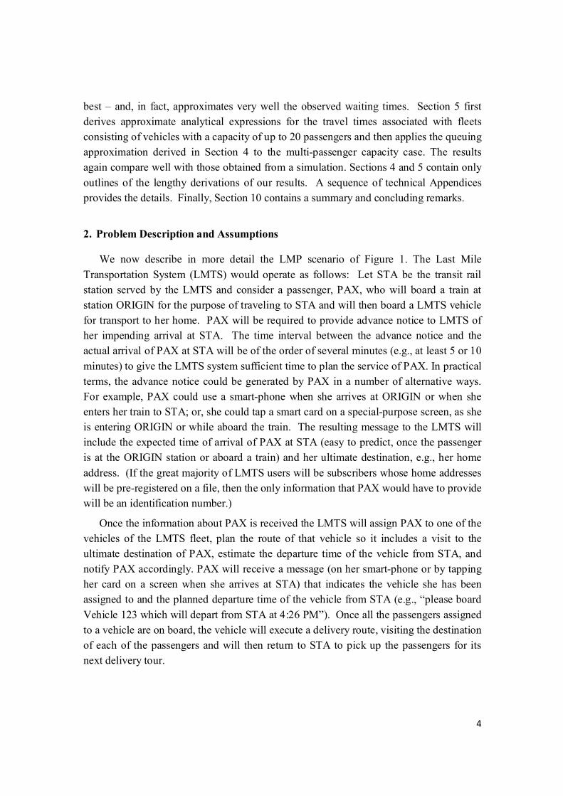
Step 2 examines this general case, in which service times are equal to the duration of delivery tours consisting of (> 1) or fewer delivery stops, as shown in Figure 3. To

Figure 3: Vehicle routes of the General-Capacity, Multi-Vehicle LMP

apply to the general capacity case the queuing expressions that were derived in Step 1, we need to compute in Step 2, the approximate length and the variance of the length of the vehicle tours shown in Figure 3. We accomplish this by using arguments from geometrical probability and from the literature on the Traveling Salesman Problem. We

8

obtain several such approximate expressions in this way and compare them with the results of another series of simple simulation experiments to select the expressions that fit best the observed expected values and variances of the vehicle tour lengths. We then use these expressions, along with the queuing-based approximation derived in Step 1, to complete the process of estimating the performance of the LMTS for the general case of arbitrary fleet size and arbitrary vehicle capacity.

Sections 4 and 5 provide only an outline of the (occasionally lengthy) derivations of the results contained therein. The reader is referred to a set of 20 Appendices for details.

4. The Unit-Capacity, Multi-Vehicle LMP

In this section we consider the analysis of the Unit-Capacity, Multi-Vehicle case, described in Section 3 as Step 1, in which = 1, and m is an arbitrary positive integer. As already indicated above (Figure 2), the length of the vehicle trips in this case is equal to two times the distance between the rail station and a customer’s destination. For the purpose of keeping relatively simple the various expressions derived, and without loss of generality, we shall assume that travel in the rectangular region of interest [Assumption (viii) in Section 2] is according to the right-angle metric, with directions of travel parallel to the sides of the rectangle. A typical route, for serving a particular customer P is indicated through a dashed line in Figure 2. Because we have also postulated [Assumption (x)] constant and unit travel speeds, the expressions for travel times in the region are identical with those derived for travel distances.

The basic notation is summarized as follows:

h = the constant headway between arrivals of trains at the station STA (and discharges of customers); = a random variable denoting the number of LMTS customers (“batch size”) discharged after the arrival of a train at STA – with the sizes of successive batches being mutually independent and with ( ) = , and (ξ) = denoting, respectively, the expected value and variance of ;

S = a random variable denoting the service time of any random LMTS customer with ( ) = and variance ( );

Note that the successive service times by any given vehicle in the fleet are independent and identically distributed. The traffic load (or utilization ratio) is given by = / ℎ. Note that / is the service rate of the LMTS, while /ℎ is the rate of customer arrivals per unit of time. Appendix 1 presents some background results that are useful in the analysis of the Unit-Capacity, Multi-Vehicle case.

9

4.1 A Lower Bound

We are particularly interested in the expected waiting time, W, of LMTS customers until they board one of the m vehicles to be transported to their eventual destination. Determining this expected waiting time, as a function of the LMTS design parameters is a critical step toward developing the means to design LMTS satisfying certain level-of-service requirements. We begin by obtaining a lower bound for W.

Since no exact analytical solution exists for the complicated / / /∞ queuing model, we consider a modified system in which, instead of having batch arrivals with average size ( ) at constant intervals (headway = h), we have a single arrival of a customer every ℎ/ ( ) units of time. This modification transforms the original / / /∞ system into a / / /∞ queuing system. The latter is characterized by a shorter average waiting time, W, than the original / / /∞ system since the arrivals of customers are deterministic and evenly distributed, while the total expected number of customers served by the two systems is the same. However, no exact analytical solution exists for the / / /∞ model either. Therefore, we consider instead a / /1/∞ model, which has identical customer inter-arrival times with the / / /∞ model, while its single server works m times faster than each of the servers of the m-server system. Following the “remaining work inequality” principle of multi-server queuing models in [9] and applying the approximation of / /1/∞ given in [7] (see Appendix 1) we can then obtain (Appendix 3) a lower bound as follows: ≥ ( ) ( ) ( ) + ℎ ( ) − 2ℎ ( )− ℎ ( )2 ( ) ℎ− ( ) ( ) ⑴

when the size of customer arrival batches, , is drawn from a General distribution and the customer service time, S, is also drawn from a General distribution.

For the special case (Appendices 2 and 4) in which the size of customer arrival batches is a Poisson random variable with intensity and the service region is a × square: ≥ −7 ℎ+ 7 ℎ+ 7 12( ℎ− ) ⑵

4.2 Two Upper Bounds

We next turn to obtaining an upper bound for W in the original Unit-Capacity, Multi-Vehicle / / /∞ model. To do this, we pre-assign customers to different vehicles and construct a corresponding single-server queuing model / /1/∞ for each vehicle, where N is the random variable indicating the number of customers from a single train assigned to the same vehicle.

With such an assignment policy, service inefficiencies exist since a customer is required to wait for his or her assigned vehicle, even when other vehicles may be

10

available. Thus, the average waiting time in this case will be larger than the average waiting time in the original model and provides an upper bound. The customer flow is shown schematically in Figure 4 below.

Figure 4 Customer flow in the pre-assignment policy

The / /1/∞ model is still difficult to work with. To obtain approximate

expressions for W, we decompose the problem into two parts (Appendix 5). First, the N customers in some batch who are assigned to the same vehicle are treated as a single “macro-customer” P. This reduces the / /1/∞ model to the more tractable / /1/∞ model and allows us to obtain an upper bound for , the expected waiting time until the first customer in P receives service. In a second step, we then compute the additional expected waiting time, , that the i-th customer in P suffers due to being preceded for service by i-1 other customers in P. Thus, the expected waiting time of a customer P is given by = + . In Appendix 5 we show that: ≤ ( ) ( ) + ( ) ( )2(ℎ− ( ) ( ))

= ( ) ( ) + ( ) ( )− ( ) ( )2 ( )

Thus the upper bound we seek is: ≤ ( ) ( ) + ( ) ( )2(ℎ− ( ) ( )) + ( ) ( ) + ( ) ( ) − ( ) ( )2 ( ) ⑶

The bound (3) is valid under general assumptions about the probability density functions of the batch size, , and the service times, S. Moreover, (3) has been derived without considering how exactly customers are assigned to vehicles. We analyze next two different policies for customer assignment to vehicles. Each of these policies will

11

provide different modified / /1/∞ models with different ( ) and ( ), leading to different expressions for and , and, ultimately, different upper bounds for W.

4.2.1 Randomized Assignment Policy

One possible policy is to assign all the customers randomly (with equal probability 1/m) and independently to the m different vehicles, with every vehicle serving individually the stream assigned to it. This is illustrated in Figure 5 below:

Figure 5 Randomized Assignment Policy

The model corresponding to the randomized assignment policy led (Appendix 6) to

the following strict upper bound for the case of a General distribution of customer batch sizes and a general distribution of customer service times: ≤ ℎ ( ) ( ) − ℎ ( ) ( ) + ( ) ( )− ( ) ( )2 ℎ− ( ) ( ) ( ) (4)

When the customer batch size is a Poisson random variable and the service region is a × square, the strict upper bound (4) becomes (Appendix 7): ≤ 7 + 6 ℎ− 6 12 ( ℎ− ) (5)

An approximate upper bound for the case of Poisson customer batch size and a square service region can also be derived. This last bound was obtained (also in Appendix 7) using an approximate expression for the average waiting time of the / /1/∞ queuing model given in [8]: ≤ 7 12( ℎ− ) ∙ exp −4( ℎ− )7 + 2 (6)

4.2.2 Cyclic Assignment Policy

Another possible policy is to assign customers in cyclic order to the vehicles: the first customer in the batch is assigned to Vehicle 1, the second to Vehicle 2, …, the (m+1)-th

12

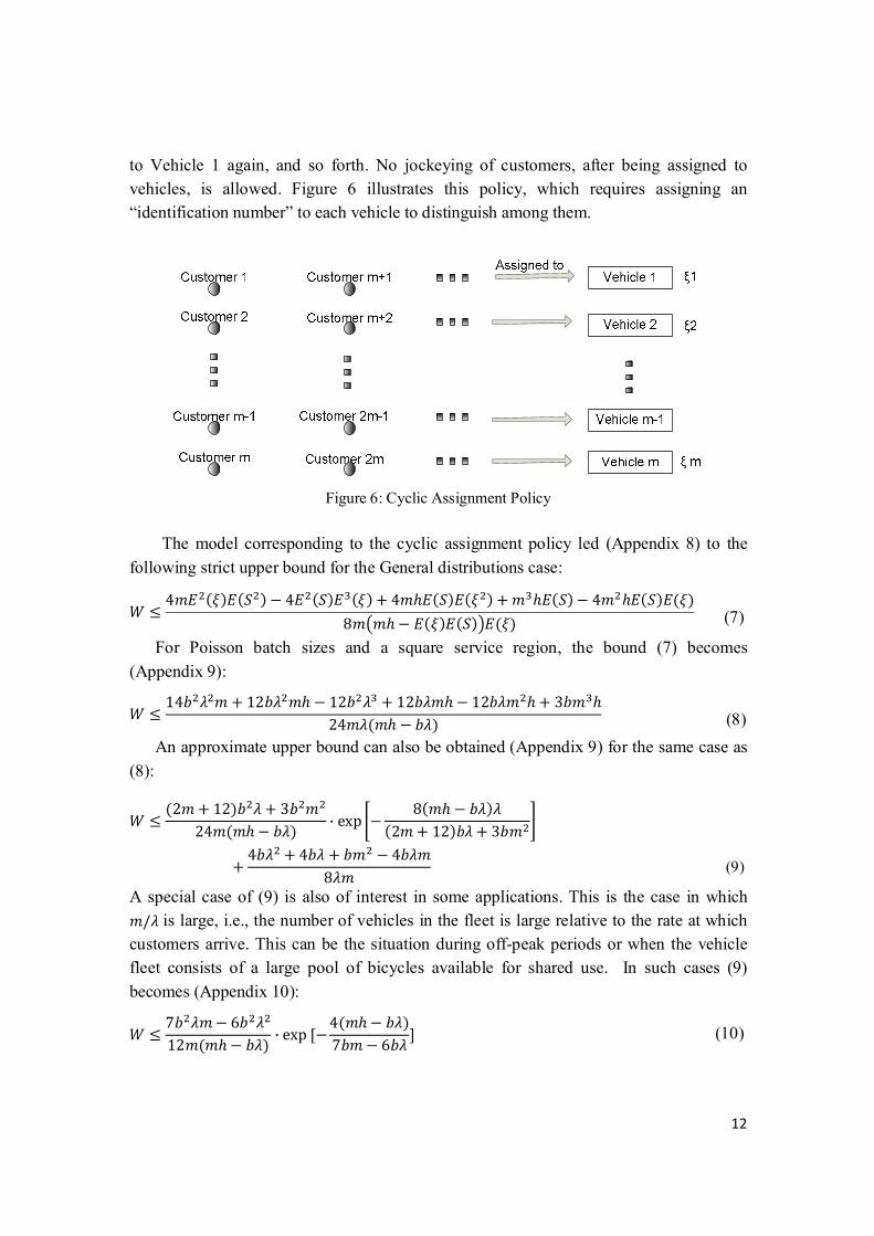
to Vehicle 1 again, and so forth. No jockeying of customers, after being assigned to vehicles, is allowed. Figure 6 illustrates this policy, which requires assigning an “identification number” to each vehicle to distinguish among them.

Figure 6: Cyclic Assignment Policy

The model corresponding to the cyclic assignment policy led (Appendix 8) to the

following strict upper bound for the General distributions case: ≤ 4 ( ) ( ) − 4 ( ) ( ) + 4 ℎ ( ) ( ) + ℎ ( )− 4 ℎ ( ) ( )8 ℎ− ( ) ( ) ( ) (7)

For Poisson batch sizes and a square service region, the bound (7) becomes (Appendix 9): ≤ 14 + 12 ℎ− 12 + 12 ℎ− 12 ℎ+ 3 ℎ24 ( ℎ− ) (8)

An approximate upper bound can also be obtained (Appendix 9) for the same case as (8):

≤ (2 + 12) + 3 24 ( ℎ− ) ∙ exp − 8( ℎ− ) (2 + 12) + 3 + 4 + 4 + − 4 8 (9)

A special case of (9) is also of interest in some applications. This is the case in which / is large, i.e., the number of vehicles in the fleet is large relative to the rate at which customers arrive. This can be the situation during off-peak periods or when the vehicle fleet consists of a large pool of bicycles available for shared use. In such cases (9) becomes (Appendix 10): ≤ 7 − 6 12 ( ℎ− ) ∙ exp [−4( ℎ− )7 − 6 ] (10)

13

The approximate upper bound (10) has the desirable property of becoming more accurate as approaches 1. Since = / ℎ , a large / means a large /ℎ when approaches 1. This corresponds to situations in which the service region is large and/or the train frequency is low.

4.3 Numerical Experiments for the Unit-Capacity, Multi-Vehicle LMP

To assess the performance of the many approximate expressions obtained in Sections 4.1 and 4.2 under a broad range of conditions, a simple simulation of the Unit-Capacity, Multi-Vehicle LMP was carried out with a program written in java. We consider a square service region with geometry / = / = 2.5 = 150 , headway of ℎ =10 = 600 , and Poisson-distributed batch sizes of = 20, 40, 60, 80. We selected these parameters so that the system would make sense physically. The respective simulation results are shown in Figures 7, 8, 9, and 10.

Figure 7: Simulation results and cyclic upper bounds of average waiting time when = 20


0.2 0.25 0.3 0.35 0.4 0.45 0.5 0.55 0.6 0.65 0.7 0.75 0.80

50

100

150

200

250

300

350

Utilization Ratio

Ave

rage

Wai

ting

Tim

e (s

ec)

h=600sec,b=150sec,Lamda=20

Simulation ResultsApproximate Cyclic Upper BoundStrict Cyclic Upper Bound

0.4 0.45 0.5 0.55 0.6 0.65 0.7 0.75 0.8 0.85 0.90

100

200

300

400

500

Utilization Ratio

Ave

rage

Wai

ting

Tim

e (s

ec)



14


Figure 10: Simulation results and cyclic upper bounds of average waiting time when = 80.

The figures plot the simulation results and our estimates for the average waiting time per customer W (in seconds) against the utilization ratio = / ℎ . Since the simulated system has Poisson customer batch size and a square service region, and / is not large, only expressions (2), (5), (6), (8), and (9) from Sections 4.1 and 4.2 are applicable and considered here.

Comparison with the simulation results led to two initial observations: first, the strict lower bound (2) is not useful, as it provides poor estimates of W, often including negative values; and, second, the strict randomized assignment upper bound (5) and the approximate randomized assignment upper bound (6) is also unreliable as it often generates very high estimates of delays. The values obtained from (5) and (6) have therefore been omitted from Figures 7-10, which only show the strict cyclic upper bound (8), the approximate cyclic upper bound (9) and the simulation results.

0.4 0.45 0.5 0.55 0.6 0.65 0.7 0.75 0.8 0.85 0.9 0.93750.93750

100

200

300

400

500

600

Utilization Ratio

Ave

rage

Wai

ting

Tim

e (s

ec)



0.4 0.45 0.5 0.55 0.6 0.65 0.7 0.75 0.8 0.85 0.9 0.950.9530

100

200

300

400

500

600

700

Utilization Ratio

Ave

rage

Wai

ting

Tim

e (s

ec)



15

As can be seen in the figures, the strict cyclic upper bound, (8), is a consistently reliable upper bound for W, while the approximate cyclic upper bound, (9), provides a very good approximation for the entire range of parameter values explored, which span the full set of conditions under which the LMTS remains stable. In a practical system, it would be desirable to achieve values of 1 to 5 minutes, for the average waiting time until passengers to board a vehicle. Note from Figures 7-10 that for this range of values (60 to 300 seconds) the difference between the approximate cyclic upper bound and the simulation results stays small in both absolute and percentage terms. For example, when = 20 (Figure 7), this difference never exceeds 30 seconds and 15% for values of W between 2 and 4 minutes. For a queuing system as analytically complicated as / / /∞ , expression (9) performs remarkably well.

We also note that it is not surprising that (9), the approximate cyclic upper bound, performs much better than (6), the approximate randomized upper bound. This is because the customers are more evenly distributed among the vehicles under the cyclic assignment policy than under the randomized assignment policy and, consequently, the variance of the service times under the former policy is much smaller than under the latter for instances of practical interest.

In conclusion, given the train frequency (batch inter-arrival times), customer arrival intensity (batch size), geometry of the service region (shape and size), distance metric (right-angle, Euclidean) and vehicle speed, we can use expressions based on the strict cyclic upper bound, (8) and the approximate cyclic upper bound, (9), to estimate LMTS system performance for any given number of unit-capacity vehicles. Section 4.4 will first demonstrate the robustness of (8) and (9) to mild changes in the assumptions under which they were obtained. In Section 5, we shall seek to extend our findings to the general case in which vehicle capacity can be greater than 1.

4.4. Sensitivity Analysis: Unit-Capacity, Multi-Vehicle LMP

In this section, we relax the assumptions concerning the shape of the service region and the continuity of the travel medium to derive expressions for W, analogous to (2), (5), (6), (8), and (9), for three specific cases: a rectangular service region; a diamond-shaped region; and a service region that includes a barrier to travel. We then repeat our simulation experiments to test the performance of the new expressions and conclude that the strict cyclic upper bound and the approximate cyclic upper bound continue to outperform the other bounds and to provide accurate approximations to W under a wide range of conditions.

4.4.1 Rectangular Service Region ( = , > 1)

16

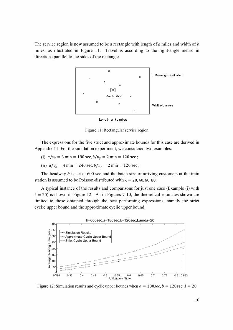
The service region is now assumed to be a rectangle with length of a miles and width of b miles, as illustrated in Figure 11. Travel is according to the right-angle metric in directions parallel to the sides of the rectangle.

Figure 11: Rectangular service region

The expressions for the five strict and approximate bounds for this case are derived in

Appendix 11. For the simulation experiment, we considered two examples:

(i) / = 3 min = 180 sec, / = 2 min = 120 sec ;

(ii) / = 4 min = 240 sec, / = 2 min = 120 sec ;

The headway h is set at 600 sec and the batch size of arriving customers at the train station is assumed to be Poisson-distributed with = 20, 40, 60, 80.

A typical instance of the results and comparisons for just one case (Example (i) with = 20) is shown in Figure 12. As in Figures 7-10, the theoretical estimates shown are limited to those obtained through the best performing expressions, namely the strict cyclic upper bound and the approximate cyclic upper bound.

Figure 12: Simulation results and cyclic upper bounds when = 180 , = 120 , = 20

0.294 0.35 0.4 0.45 0.5 0.55 0.6 0.65 0.7 0.75 0.8 0.8330

50

100

150

200

250

300

350

400

Utilization Ratio

Ave

rage

Wai

ting

Tim

e (s

ec)

h=600sec,a=180sec,b=120sec,Lamda=20


17

For Example (i), i.e., for k = 1.5, and for values of the average waiting time of the order of 1 to 4 minutes, the percent difference between the approximate cyclic upper bound and the simulation results was of the order of 10-25% for the entire range of values of (= 20, 40, 60, 80). For Example (ii), i.e., for k = 2, = 240 , = 120 , this increased to 20-35%. Thus, as k becomes larger and the service region more elongated, the approximate cyclic upper bound becomes less accurate. This is because this approximate bound is sensitive to the variance of the service times which, in turn, increases as the region becomes more elongated and resembles a rectangular strip. The bound’s accuracy is, however, relatively insensitive to the customer demand intensity .

4.4.2 Diamond Service Region with Side of Length b

In the next sensitivity test, the service region is assumed to be a perfect four-sided diamond with side equal to b miles, as illustrated in Figure 13. The theoretical results for this case are derived in Appendix 12.

Side=b miles

Rail Station

Passenger destination

Figure 13: Four-sided diamond service region

In the simulation and numerical comparisons we considered a service region such that / = / = 2.5 min = 150 sec, with a headway of ℎ = 10 min = 600 sec, and Poisson-

distributed customer batch sizes with = 20, 40, 60, 80. Comparisons with the simulation results, when = 20, are shown in Figure 14.

18

Figure 14: Simulation results and cyclic upper bounds of diamond service region when =150 , = 20

For average waiting times of the order of 1 to 4 minutes, the percent difference between the approximate cyclic upper bound and the simulation results was of the order of 10-20%. The accuracy of the bound is insensitive to the customer demand intensity .

4.4.3 Rectangular Service Region with Barrier

The service region is next assumed to be rectangular service region that contains an impenetrable barrier to travel. The geometry of the barrier is shown in Figure 15. Appendix 13 contains the theoretical derivations for this case.

Figure 15: Rectangle service region with barrier inside

In the simulation and numerical comparisons we considered a service region such that / = 2.5 = 150 , / = 2 min = 120 sec , / = 0.625 min = 37.5 sec , / = 0.5 min = 30 sec , / = 0.25 min = 15 sec, with headway of ℎ = 10 min = 600 sec,

and Poisson-distributed passenger batch sizes of = 20, 40, 60, 80. The simulation results when = 20 are shown in Figures 16.

0.248 0.3 0.35 0.4 0.45 0.5 0.55 0.6 0.65 0.7 0.75 0.8 0.85 0.9 0.9430

100

200

300

400

500

600

700

800

Utilization Ratio

Ave

rage

Wai

ting

Tim

e (s

ec)

Diamond region,h=600sec,b=150sec,Lamda=20


19

Figure 16: Simulation results and cyclic upper bounds, rectangle service region with barrier, when = 20.

For average waiting times of the order of 1 to 4 minutes, the percent difference

between the approximate cyclic upper bound and the simulation results was again of the order of 10-20%, and the accuracy of the bound was insensitive to the customer demand intensity .

Overall, the sensitivity analysis of this section, suggests that the strict cyclic upper bound and the approximate cyclic upper bound remain valid and provide good estimates of performance for a wide range of customer demand rates and for differently shaped compact and convex service regions.

5. General-Capacity, Multi-Vehicle LMP: Upper Bounds and Approximations

In this section we consider the General-Capacity, Multi-Vehicle LMP, in which both the vehicle capacity, c, and the number of vehicles, m, are arbitrary positive integers. The vehicles will now travel along more complicated routes than in the = 1 case to deliver customers to their destinations. In practice, one would expect the vehicle capacity to be a small number of the order of 4 to 10 customers – unless the LMTS fleet consists of bus-size vehicles, in which case the methodologies laid out in this paper are less applicable.

As explained in Section 3, the General-Capacity, Multi-Vehicle LMTS will be viewed as a spatially distributed queuing system in which the service times are equal to the amount of time it takes to complete a customer delivery tour and return to the train station – see also Figure 3. Vehicle routing and path choice issues must therefore be addressed in this connection. This is done in this section, which also summarizes the bounds and approximations we have obtained.

The approach to be described consists of the following three steps: (i) customers are partitioned into clusters with the size of each cluster no larger than the vehicle capacity, c;

0.243 0.3 0.35 0.4 0.45 0.5 0.55 0.6 0.65 0.7 0.75 0.8 0.85 0.90.9250

100

200

300

400

500

600

700

Utilization Ratio

Ave

rage

Wai

ting

Tim

e (s

ec)

Barrier,h=600sec,a=150sec,b=120sec,d=37.5sec,e=30sec,f=15sec,Lamda=20


20

(ii) each cluster is assigned to a vehicle and a delivery route is designed for each vehicle; (iii) using the service times (i.e., tour durations) computed in the previous step, the (appropriately modified) queuing results from the Unit-Capacity model of Section 4 are then applied to estimate system performance. The performance measures we shall concentrate on include average waiting time until boarding a vehicle and average time until delivery to destination, i.e., the sum of the time spent waiting to board a vehicle and of the time spent riding until delivery.

5.1 Approximating the Expectation and Variance of Tour Lengths

Since we are looking for widely applicable approximations and bounds on system performance and not for exact expressions, we have selected a “greedy” partitioning strategy for assigning customers to vehicles. Specifically, we partition customers in each arriving batch simply according to their order of arrival at the station. In other words, Vehicle 1 serves customers 1, 2,…, c in a single tour, Vehicle 2 serves customers c+1, c+2,…, 2c in a single tour, and so on. If we consider the c customers served by one vehicle as a single request for service, the number of service requests after the arrival of each train is given by / , when the size of an arriving batch is .

For the routing step, we also use a “greedy routing strategy” – which, however, is refined subsequently, in the manner described later in this section. Upon leaving the rail station with c customers on board, the vehicle will first deliver the customer whose destination is closest to the station, denoted as Point A in Figure 17, then the customer whose destination is closest to point A (i.e., Point B in Figure 17) and so forth. Finally, after delivering the last customer (Point F) the vehicle will return to the rail station. Thus, we construct a vehicle tour using essentially a “Nearest Neighbor” (NN) heuristic approach. The reason for following this sub-optimal routing strategy is that it is mathematically feasible to compute approximately both the expected length and the variance of the length of a NN tour that delivers c customers and returns to the rail station. Both of these quantities (expected length and variance of the length) are necessary if one is to apply the queuing expressions derived in Section 4.

A better alternative would have been to find the Hamiltonian tour, i.e., the optimal “Traveling Salesman” tour (TST), through the c + 1 points (customer destinations plus rail station) to be visited. However, we are not aware of any simple explicit expressions for the variance of the length of TST tours. We have therefore opted for the NN-based routing approach. We have, however, attempted to correct the expressions for “expected length” and “variance of length” derived through the NN-based approach, by comparing these with corresponding estimates (expectation and variance) obtained through many numerical experiments.

21

Figure 17: Greedy routing strategy for the General-Capacity, Multi-Vehicle LMP

The tour shown in Figure 17 consists of one First Leg, c-1 Middle Legs, and one Last

Leg. The expected length of the entire route is then given by ( ) = + , +⋯+ , + (11) where the notation and denotes, respectively, the expected length of the first and last legs of the tour, while , denotes the expected distance between the destination of the last customer delivered and the nearest destination of k remaining customers still to be delivered. For example, , denotes the distance between the first of the customers delivered (i.e., the nearest one to the rail station) and the nearest destination among the destinations of the remaining c-1 customers still to be delivered.

The variance of the length of the entire service route can be similarly approximated as = + , +⋯+ , + , (12)

where denotes a variance and the subscripts can be interpreted in exactly the same way as the subscripts of the expectations, s, above. Finally, the second moment of the length of the entire service tour is given by = ( ) = + ( ( )) .

The above estimates of the moments and variance of the service tour can be converted into time units, if one is given information about the speed of travel in the region of interest. To simplify this conversion, we shall continue to assume here that travel speed is constant throughout the region.

We have derived approximate expressions for ( ), , and assuming a right-angle travel metric and a rectangular service region of size × . With the NN (“greedy”) routing strategy, the length of the first leg of the delivery tour is the distance from the rail station to the nearest of c random points (c random customer destinations), while the last leg is the distance from another (approximately) random point (the

22

destination of the final customer served in the tour) back to the rail station. It is not difficult to derive the expectation and variance of these distances as shown in Appendices 14 and 15, respectively.

The length of any middle leg is equal to the distance between a random point (the destination of the most recently delivered customer) and the nearest destination of anyone of the customers who still remain on the vehicle. Computing the expected value and variance of this distance is a far more complicated and tedious problem due to the effects of the region’s boundaries. We pursued two different approaches for approximating these quantities using: (a) a Crofton Approximation (Appendix 16) that computes the expected distance and variance of the distance between a random point and the closest of N (N=1, 2, 3,…, c-1) other random points on a linear segment using Crofton’s Method[7] and then treats the distances in the horizontal and vertical directions, as if they are independent; and (b) a Center Approximation (Appendix 17) that relies on computing the expected value and variance of the distance between the center of the rectangular service region and the closest of N (N=1, 2, 3,…, c-1) random points in the rectangle.

We then tested the analytical expressions derived through (a) and (b) by means of an extensive series of numerical experiments, described in Appendix 18. The experiments indicated that the expressions performed equally well, but we have chosen to use the Crofton Approximation henceforth because of its simpler form. We have also used a linear regression model to correct the Crofton and Center expressions, so they fit better with the numerical observations. It was found that, again, both of the corrected expressions perform roughly equally and will use henceforth the Crofton Approximation with the regression correction because of its simpler form.

In conclusion, our best estimates for the first and second moments of the length of a middle leg of the delivery tour, given that N customers remain to be delivered, are given by the following expressions: , ≈ , = ( + 3)( + )2( + 1)( + 2) (13)

, ≈ , = ( + 7)( + )2( + 1)( + 2)( + 3) + 2( + 32( + 1)( + 2)) (14)

After correcting these expressions through regression, they become: , ≈ , ≈ (1.13047 + 0.099945 ) ∙ ( + 3)( + )2( + 1)( + 2) (15) , ≈ , ≈ (0.525751 + 0.372122 ) ∙ ( ( + 7)( + )2( + 1)( + 2)( + 3)+ 2 + 32( + 1)( + 2) (16)

23

The detailed mathematical derivation of (13) and (14) is in Appendix 16 and of (15) and (16) in Appendix 18.

5.2 Completion of the Queuing Model

In this subsection, we incorporate the results of the above Section 5.1 into the previously (Section 4) derived results for the Unit-Capacity queuing model to obtain approximations of system performance for the General ( > 1) Capacity case. Specifically, we use the expressions for the length and duration of customer delivery tours when > 1 , to estimate the service times for the General Capacity model and use these estimates in the various expressions for the expected waiting time until boarding a vehicle that were obtained in Section 4.2.2 under the cyclic assignment policy. As was demonstrated in Section 4.3, these latter expressions approximate best the observed (through simulation) system performance.

For the case of a General distribution for the size of customer batches and of General service times the strict cyclic upper bound [cf. expression (7)] and the approximate cyclic upper bound [cf. expression (9)] for the waiting time until boarding a vehicle (see Appendix 19 for details) is then given by: , ≤ 4 ( ) − 4 ( ) ( ) + 4 ℎ ( ) + ℎ ( ) − 4 ℎ ( ) ( )8 ℎ− ( ) ( ) ( )

(17)

, ≈ + ( )2(1 − ) ∙ exp −2(1 − )(1− ) 3 + + ( ) ∙ 4 + − 4 ( ) 8 ( ) (18)

When the size of customer batches has a Poisson distribution, and the duration of the delivery service tour is approximated through Crofton’s method (without using the regression correction), the various terms of (17) and (18) above take the following values: ( ) ≈ ( ) , ( ) ≈ 4 ( ) + 4 , = 0, = ( ) ( ) ℎ , ( ) = ( ) ( ) , = 4 ( ) ( ) + 4 ( ) ( ) + ( ) 4 ( ) ( ) , Hypergeometric2F1 = ( , ; ; ) = ( ) ( ) ( ) ⁄ !⁄

24

( ) = 2 (1 + (1 + 2 )Hypergeometric2F1[1,−1 − , 12 ,−1])1 + 3 + 2 + ( + 3) ( + 1)( + 2) + 2

= 2 (1 + 2 + 2 )1 + 3 + 2 − 2 (1 + (1 + 2 )Hypergeometric2F1[1,−1 − , 12 ,−1]) (1 + 3 + 2 ) + + 11 + 19 + 12( + 1) ( + 2) ( + 3) + 7 24

Note that in (17) and (18) we have used the notation , and , for the expected waiting time until a customer will board a vehicle, while in (7) and (9) we used the notation W in (7) and (9) for the same quantity. This is because we also want to introduce here another quantity, , which is defined as the expected time a customer will spend riding on the vehicle before being delivered to his destination. Considering the riding component of the trip, the total expected time from the instant a customer arrives at the rail station until she is delivered at her destination is given by = +

where

= 2 (1 + (1 + 2 )Hypergeometric2F1[1,−1− , 12 ,−1])1 + 3 + 2 + − 1 + 1

as shown in Appendix 19.

5.3 Simulation and Comparisons for the General-Capacity, Multi-Vehicle LMP

To assess the validity of the expressions developed in Section 5.2, a simple simulation of a General-Capacity, Multi-Vehicle LMTS was carried out with a program written in java. We consider a square service district with geometry / = / = 2.5 = 150 , headway between train arrivals of ℎ = 10 = 600 , vehicle capacity c = 3, 5 or 9 and customer arrivals with batch size described by a Poisson distribution with = 40, 80 and 120. These parameters were selected so that the system would make sense physically. Near-optimal vehicle tours were generated by using a Traveling Salesman algorithm. Specifically, the simulation generated sets of c points, randomly and independently distributed in the square according to a uniform distribution, and a Traveling Salesman tour through these points was drawn through an algorithm that is known to generate near-optimal solutions. The algorithm implements a tour-improvement heuristic that begins with an initial solution and then improves that solution through arc exchanges (“2-exchange” heuristic) and through changes in the sequencing of the nodes in the tour (“node insertion” heuristic). More details are provided in Appendix 20 that describes the simulation experiments.

25

Figures 18 through 22 present a sample of comparisons between the simulation results and the analytical approximations of Section 5.2 for the following respective cases: = 3, = 40; = 3, = 80; = 3, = 120; = 5, = 80; and = 9, = 120.

Figure 18 Simulation and analytical results when = 3 and = 40



0.4 0.45 0.5 0.55 0.6 0.65 0.7 0.75 0.8 0.850

50

100

150

200

250

300

350

400

450

Utilization Ratio

Ave

rage

Wai

ting

Tim

e (s

ec)

b=150sec,h=600sec,c=3,Lamda=40

Strict UB no regression until BoardApprox no regreesion until BoardSimulation unitl BoardStrict UB no regression until DeliveryApprox no regreesion until DeliverySimulation unitl Delivery

0.65 0.7 0.75 0.8 0.85 0.90

100

200

300

400

500

600

Utilization Ratio

Ave

rage

Wai

ting

Tim

e (s

ec)



0.72 0.74 0.76 0.78 0.8 0.82 0.84 0.86 0.88 0.9 0.92

100

200

300

400

500

600

Utilization Ratio

Ave

rage

Wai

ting

Tim

e (s

ec)



26



The horizontal axis in Figures 18-22 shows the utilization ratio = ( ) ( )/ ℎ,

while the vertical axis shows the expected waiting time until boarding a vehicle and the expected total time spent between arrival at the station and delivery at customer’s destination. A comparison of the simulation results with the estimates generated through the analytical expressions of Section 5.2 indicated that the expressions that do not include a correction for the length of delivery tours (see (13) and (14)) actually perform better than the expressions that include the correction (see (15) and (16)). The explanation for this seemingly surprising observation lies in the fact that, in the absence of the correction, (13) and (14) will underestimate the expected service time (= duration of delivery tour and its second moment). This compensates for and balances out other parts of the analysis that overestimate the service time and leads to a more accurate overall approximation. Following our practice of showing only the best-performing approximations, Figures 18 – 22 therefore show only the estimates obtained through the

0.6 0.65 0.7 0.75 0.8 0.85 0.90

100

200

300

400

500

600

Utilization Ratio

Ave

rage

Wai

ting

Tim

e (s

ec)


Strict UB no regression until BoardApprox no regreesion until BoardSimulation unitl BoardApprox no regreesion until DeliverySimulation unitl DeliveryStrict UB no regression until Delivery

0.7 0.75 0.8 0.85 0.9 0.950

100

200

300

400

500

600

700

800

Utilization Ratio

Ave

rage

Wai

ting

Tim

e (s

ec)

b=150,h=600,c=9,Lamda=120


27

strict cyclic upper bound (expression (17)) and the approximate cyclic upper bound (expression 18) that do not include a correction term.

When it comes to the expected waiting time until boarding a vehicle, both the strict cyclic upper bound and the approximate cyclic upper bound perform very well for small vehicle size. For instance, when = 3 and = 5 and customer arrival intensity of 40, 80, and 120, the difference between the simulated average time until boarding and the analytical expression is of the order of 15% or less for values between 1.5 and 4 minutes, which are the most reasonable waiting time to aim for in practice. Even when the average waiting time is smaller the difference typically stays below 25%, or less than 20 seconds.

As vehicle size increases, the accuracy of the approximation of expected waiting time until boarding declines. The reason is that, when the capacity of the vehicles is large, the performance of the system becomes increasingly unstable: for example, a change of even 1 in the number of available vehicles, from some value m to m+1, may result in a system transition from being nearly-saturated to being underutilized.

Turning to the estimation of expected total time until delivery, the analytical expressions work well for both small and large vehicles and for the broad range of customer arrival intensities ( = 40, 80, and 120) examined. This can be seen in all the Figures 18 – 22. The approximation accuracy decreases somewhat as vehicle capacity gets larger, but is still good (difference less than 30% for reasonable values of total time to delivery even when = 9).

6. Conclusion

This paper has developed a set of fully analytical expressions to support the approximate estimation of the performance of a quite general version of a Last-Mile Transportation System (LMTS). Given a lengthy list of inputs about the system’s characteristics (headways between arrivals of trains at the rail station, size of “batches” of customers on each train, number of vehicles in the service fleet, capacity of each vehicle, dimensions and travel-related properties of the urban district served), the expressions we have developed estimate the expected waiting time until a customer can board a vehicle, and the expected time between arrival at the rail station and delivery to the customer’s destination. A number of simple simulation experiments suggest that the best-performing of the expressions we have developed approximate remarkably well the expected performance of LMTS under a broad range of conditions typical of what one may encounter in practice.

On the methodological side, the principal contribution of this research is the development of several alternative approaches for bounding and approximating the

28

performance of a very difficult type of queuing system involving batch arrivals and requiring the simultaneous consideration of routing and queuing issues and the use of geometrical probability arguments. On the practical side, we believe that the analytical expressions we have developed can be very useful in designing LMTS, specifically in determining resource requirements for these systems, such as how many vehicles would be necessary to achieve a specified level of service and how many kilometers per day these vehicles would travel.

Future work will focus on improving the approximation accuracy for General-Capacity, Multi-Vehicle LMTS, by using a more sophisticated demand clustering and partitioning strategy and by expanding the range of the simulation inputs so that a broader range of conditions can be observed. A second area is to develop a simple set of unified guidelines for LMTS design and operation and apply these guidelines to the planning of a small actual experimental system, possibly to be implemented in a part of Singapore.

References

[1]. D. J. Bertsimas, G. van Ryzin, A stochastic and dynamic vehicle routing problem in the Euclidean Plane, Operation Research 39 (1991) 601-615. [2]. D. J. Bertsimas, G. van Ryzin, Stochastic and dynamic vehicle routing in the Euclidean plane with multiple capacitated vehicles, Operation Research 41 (1993) 60-76. [3]. M.R. Swihart, J.D. Papastavrou, A stochastic and dynamic model for the single-vehicle pick-up and delivery problem, European Journal of Operation Research 114 (1999) 447-464. [4]. R. Baldacci, V. Maniezzo, A. Mingozzi, An exact method for the car pooling problem based on Lagrangean column generation, Operation Research Vol. 52, No.3 (2004) 422-429. [5]. J-F Cordeau, G. Laporte, The dial-a-ride problem: models and algorithms, Ann Operation Reserch (2007) 153:29-56. [6]. D.P. Bertsekas, J.N. Tsitsiklis, Introduction to Probability, Massachusetts Institute of Technology, 2008. [7]. R.C. Larson, A.R. Odoni, Urban Operation Research, Prentice-Haill, Englewood Cliffs, NJ, 1981. [8]. W. Kramer, M. Langenbach-Belz, Approximate Formulae for the Delay in the Queueing, System GI/G/1, 8th ITC, Melbourne, 1986.

29

[9]. D. Gross, J. Shortle, J. Thompson, and C. Harris, Fundamentals of Queueing Theory, 4th edition, Wiley Series in Probability and Statistics, 2008. [10]. H. Akimaru, K. Kawashima, Teletraffic: Theory and Applications, 2nd Edition, Springer, 1993. [11]. G. Choudhury, Analysis of the M(x)/G/1 queueing system with vacation times, The Indian Journal of Statistics 2002, Volume 64, Series B, Pt.1, 37-49 [12]. W. Whitt, The Queueing Network, The Bell System Technical Journal, Vol.62, No.9, November 1983, 2807. [13]. O.J. Boxma, etc, Approximations of the Mean Waiting Time in an M/G/s Queueing System, Operation Research, Vol.27, No.6. November-December, 1979, 1115-1127. [14]. T. Kimura, Diffusion Approximation for an M/G/m Queue, Operation Research, Vol.31, No.2, March-April, 1983, 304-321. [15]. J-J Jaw, A.R. Odoni, H.N. Psaraftis, N.H. Wilson, A Heuristic Algorithm for the Multi-Vehicle Advance Request Dial-a-Ride Problem with Time Windows, Transportation Research part B, Vol.20B, No.3, 1986, 243-257.

Approximating the Performance of a Last Mile...

Documents

Transcript of Approximating the Performance of a Last Mile...