©

June 28, 2017

A hybrid line list for CH4 and hot methane continuumSergei N. Yurchenko⋆1, David S. Amundsen2, 3, 4, Jonathan Tennyson1, and Ingo P. Waldmann1

1 Department of Physics and Astronomy, University College London, London WC1E 6BT, United Kingdom2 Astrophysics Group, University of Exeter, Exeter, EX4 4QL,United Kingdom3 Department of Applied Physics and Applied Mathematics, Columbia University, New York, NY 10025, USA4 NASA Goddard Institute for Space Studies, New York, NY 10025, USA

June 28, 2017

ABSTRACT

Aims. Molecular line lists (a catalogue of transition frequencies and line strengths) are important for modelling absorption andemission processes in atmospheres of different astronomical objects, such as cool stars and exoplanets. In order to be applicable forhigh temperatures, line lists for molecules like methane must contain billions of transitions, which makes their direct (line-by-lineusage) application in radiative transfer calculations impracticable. Here we suggest a new, hybrid line list format tomitigate thisproblem, based on the idea of temperature-dependent absorption continuum.Methods. The line list is partitioned into a large set of relatively weak lines and a small set of important, stronger lines. The weakerlines are then used either to construct a temperature-dependent (but pressure-independent) set of intensity cross sections or are blendedinto a greatly reduced set of ‘super-lines’. The strong lines are kept in the form of temperature-independent EinsteinA coefficients.Results. A line list for methane (CH4) is constructed as a combination of 17 million strong absorption lines relative to the referenceabsorption spectra and a background methane continuum in two temperature-dependent forms of cross sections and super-lines. Thisapproach significantly eases the use of large high temperature line lists as the computationally expensive calculationof pressure-dependent profiles (e.g. Voigt) only need to be performed fora relatively small number of lines. Both the line list and cross sectionswere generated using a new 34 billion methane line list (known as 34to10), which extends the 10to10 line list to higher temperatures(up to 2000 K). The new hybrid scheme can be applied to any large line lists containing billions of transitions. We recommend usingsuper-lines generated on a high resolution grid based on a resolving power ofR = 1,000,000 to model the molecular continuum as amore flexible alternative to the temperature-dependent cross sections.

Key words. molecular data - line:profiles - opacity - infrared: stars - infrared: planetary systems - methods: numerical

1. Introduction

Methane is one of the key absorbers in the atmospheres of exo-planets and cool stars. Due to a large number of relatively stronglines (up to several billion) at high temperatures, the calculationof cross sections becomes extremely computationally expensive.The contribution of each line to the total absorption must betaken into account by summing their individual cross sections,usually computed using Voigt profiles, on a grid of wavelengths.To make radiative transfer calculations using these line lists moretractable the line lists are usually converted into pre-computedtables of temperature- and pressure-dependent cross sections,or k-coefficients, for specific atmospheric conditions (tempera-ture, pressure, broadeners) (Amundsen et al. 2014; Malik etal.2017). Subsequent radiative transfer calculations interpolate inthese tables. However, the calculation of these cross sectionsandk-coefficients still requires the contributions of all lines tobe summed, if only once for each atmospheric condition. Bothpre-tabulated cross sections andk-coefficients are less flexiblethan a line-by-line approach, but are computationally moreeffi-cient.

As part of the ExoMol project (Tennyson & Yurchenko2012) we produced an extensive line list for methane (12CH4),called 10to10 (Tennyson & Yurchenko 2012), containing al-most 10 billion transitions. The line list was constructed to de-

⋆ The corresponding author: Sergei N. Yurchenko; E-mail:s.yurchenko@ucl.ac.uk

scribe the opacity of methane for temperatures up to 1500 K.The 10to10 line list has been shown to be important formodelling the atmospheres of brown dwarfs and exoplan-ets (Yurchenko et al. 2014; Canty et al. 2015; Amundsen et al.2016), and has been used as an input in a number ofmodels such as TauREX (Waldmann et al. 2015b,a), NEME-SIS (Irwin et al. 2008), VSTAR (Bailey & Kedziora-Chudczer2012; Yurchenko et al. 2014), ATMO (Tremblin et al. 2015;Tremblin et al. 2016; Drummond et al. 2016), and the UK MetOffice global circulation model (GCM) when applied to hotJupiters (Amundsen et al. 2016). The ExoMol database con-tains line lists for about 40 other molecular species and hasrecently been upgraded (Tennyson et al. 2016). The line listsfor polyatomic molecules usually contain more than 10 bil-lion lines; examples include phosphine (PH3) (Sousa-Silva et al.2015), hydrogen peroxide (H2O2) (Al-Refaie et al. 2015a),formaldehyde (H2CO) (Al-Refaie et al. 2015b), and SO3(Underwood et al. 2016) (see also our review of molecular linelists Tennyson & Yurchenko 2017).

A promising alternative to the line-by-line approach was re-cently proposed by Hargreaves et al. (2015), where an accurateexperimental line list of the strongest CH4 transitions was com-plemented by a set of experimental quasi-continuum cross sec-tions, measured for a set of different temperatures. Rey et al.(2016) recently proposed an alternative, super-line (SL),ap-proach to speed up the line-by-line calculations. The idea is tobuild intensity histograms from transition intensities binned for a

Article number, page 1 of 9

Article published by EDP Sciences, to be cited as https://doi.org/10.1051/0004-6361/201731026

given temperature into wavenumber grid points. Each wavenum-ber bin is then treated as a super-line for computing cross sec-tions for different line profiles, which brings the computationalcost of a line-by-line approach almost down to that using pre-tabulated cross sections. The serious disadvantage, however, isthat only very simplistic line profiles, i.e. ones which do not de-pend on quantum numbers, can be used. Indeed, each super-lineloses memory of its upper and lower states; only the wavenum-ber is preserved. This is not a problem for the Doppler profileas it does not depend on quantum numbers. However, pressure-dependent profiles such as Voigt profiles often show strong de-pendence on the rotationalJ and other quantum numbers, whichcannot be modelled using the SL approach.

In the present work we combine these two approaches andprovide a synthetic hybrid line list for methane using the fol-lowing compilation of data: (i) a line list of strongNstr linesgiven explicitly using the ExoMol format (Hill et al. 2013;Tennyson et al. 2016) and (ii) all otherNweak weak lines con-verted into a temperature-dependent but pressure-independentbackground continuum. Thus the aim of this work is to selectthe most important lines (both the strongest and most sensitiveto the variation of line profiles with pressure and broadener) forthe direct line-by-line treatment, while the rest are processed ei-ther as cross sections or as super-lines (Rey et al. 2016). The hy-brid approach is able to retain the key features of line listsand tosignificantly ease the computation of total cross sections and k-coefficient tables (including both weak and strong lines). We in-vestigate two approaches to represent the temperature-dependentcontinuum: using pressure-independent cross sections describedby the Doppler profile and using the profile-free histograms(super-lines).

As demonstrated by Rey et al. (2014) and Nikitin et al.(2017), in order to extend the temperature coverage of the 10to10CH4 line list, the lower state energy threshold should be in-creased with respect to that used by Yurchenko & Tennyson(2014). Our 10to10 line list was based on the lower state en-ergy thresholdE lower

max = 8000 cm−1, which was estimated to besufficient for temperatures up to 1500 K. In this work we extendthe 10to10 line list by increasingE lower

max to 10,000 cm−1, whichshould extend the temperature coverage to about 2000 K. To beconsistent with the extension of the lower state energy thresh-old, the rotational coverage had to be increased from the valueof Jmax = 46 used by Yurchenko & Tennyson (2014) to aboutJmax = 50. The cost of this improvement, however, is a dramaticincrease in the number of lines, from 9.8 billion to 34 billion.The resulting ‘34to10’ line list is used in this work to buildacontinuum absorption model for methane as described above.

The partitioning of the 34 billion line list into a set ofNstrstrong lines andNweak weak lines is presented in Section 2,where we also define and test the strong/weak partitioning. InSection 3 our continuum model is tested by comparing it to thetraditional approach of explicitly summing up the cross sectioncontributions from all lines, at different temperatures and pres-sures. Section 4 presents our final results.

2. Strong/Weak line list partitioning

In the following, the new line list for methane, which wehave named 34to10, is used in all our examples. The line listis an extension of the 10to10 line list, produced using thesame computational approach (Yurchenko & Tennyson 2014) byextending the lower state energy range from 8,000 cm−1 to10, 000 cm−1. Calculations were performed with nuclear mo-tion code TROVE (Yurchenko et al. 2007). As before, here cal-

culations used a spectroscopically determined potential energysurface (Yurchenko & Tennyson 2014) and ab initio dipole mo-ment surfaces (Yurchenko et al. 2013). The new line list con-tains 8,194,057 energies below 18,000 cm−1 and 34,170,582,862transitions covering rotational excitations up toJmax = 50. Thecalculation of the additional 28 billion transitions took approx-imately 5 million CPU hours on the Cambridge High Perfor-mance Computing Cluster Darwin. The wavenumber coverage,however, is kept the same as in the 10to10 line list, which meansthat the region from 10,000 to 12,0000 cm−1 is less completefor the target temperature of 2000 K. All other computationalcomponents (potential energy and dipole moment surfaces, ba-sis sets, etc.) are the same as in Yurchenko & Tennyson (2014).

In order to mitigate the difficulty of using such an extremelylarge line list, we proposed dividing it into two subsets, respon-sible for strong and weak absorptions. The first question is howto define and separate ‘strong’ and ‘weak’ transitions. The largedynamic variation of the methane intensities means that a singleintensity threshold would be not optimal. The following factorswere taken into consideration when defining the intensity parti-tioning thresholds:

(i) In regions of very strong bands many lines with moderateintensities are barely visible, while weak lines which lie betweenthe main bands can be relatively important;

(ii) The definition of ‘strong’ and ‘weak’ must betemperature-dependent as ‘hot’ bands, which are weak at lowtemperatures owing to the Boltzmann factor, become strongerwith increasing population of excited lower states at higher tem-peratures;

(iii) At the same time, the intensities of the fundamentals andovertones decrease with temperature owing to the decrease intheir relative populations (e.g. due to a larger partition function);

(iv) Finally, even relatively weak lines at longer wavelengthsare very sensitive to pressure variations, due to their lower den-sity.

To aid in the strong/weak partitioning, we introduced a refer-ence CH4 opacityαref(ν) based on two temperatures,T1 = 300 KandT2 = 2000 K, and two pressures,P1 = 0 bar andP2 = 50 bar,on a wavenumber grid of∆ν = 1 cm−1 (ν = 0 . . .12000 cm−1)by choosing the maximum cross section value among these fourat each wavenumber grid pointk:

αref(νk) = max(αP=0300 , α

P=02000, α

P=50300 , α

P=502000). (1)

The reference average intensities (cm/molecule) can then be de-fined as

I(νk) ≡ αref(νk)∆ν. (2)

Figure 1 shows the reference cross section curve used here forthe 34to10 line list.

We then define the strong/weak partitioning using two crite-ria, one dynamic and one static. According to the static criterion,all lines stronger than the thresholdIthr are automatically takeninto the strong section (e.g.Ithr = 10−25 cm/molecule). The dy-namic criterion characterizes the line ˜ν f i from the wavenumberbin k (ν f i ∈ [νk − 0.5 cm−1, νk + 0.5 cm−1]) as strong if all fourreference absorption intensities are stronger than the reference(average)Iνk intensity by some scaling factorCscale(e.g. strongerthan 10−5 × Iνk ). The scaling factorCscale is made wavenumber-dependent using the following exponential form, also showninFig. 2:

Cscale(ν) = 10−5 ×[

1− 0.9e−0.0005ν]

. (3)

Article number, page 2 of 9

0 2000 4000 6000 8000 10000 1200010-28

10-26

10-24

10-22

10-20

10-18

wavelength, m

300 K, 0 bar300 K, 10 bar2000 K, 0 bar2000 K, 10 bar

cros

s se

ctio

ns, c

m2 /m

olec

ule

0.831.001.251.672.02.54.05.0 10.0

7000 7050 7100 7150 7200 7250 7300 7350 74000

1x10-22

2x10-22 300 K, 0 bar300 K, 10 bar2000 K, 0 bar2000 K, 10 bar

wavenumber, cm-1

Fig. 1. Reference cross sections obtained using the Doppler profileatT = 300 K andT = 2000 K on the uniform∆ν = 10 wavenumber grid.The green line (T = 2000 K andP = 0 bar) is almost identical to theblue line (T = 2000 K andP = 50 bar) at this region and for this scale,and thus can be barely seen.

This scaling is necessary to take into account the importance ofthe varying density of lines at different spectroscopic regions forthe accurate description of the line profiles: the smaller numberof lines at the longer wavelengths means the cross sections aremore sensitive to the shape of the profiles and to the samplingof the grid points. At the shorter wavelengths the spectrum issmoothed out by the large number of overlapping lines, whichistherefore less sensitive to these factors. With this expression wethus assume a quasi-exponential increase in the density of linesvs wavenumber, or, colloquially, a quasi-exponential decrease intheir importance.

0 2000 4000 6000 8000 10000 120000.0

5.0x10-6

1.0x10-5

1.5x10-5

dyna

mic

sca

ling

fact

or

wavenumber, cm-1

Fig. 2. Dynamic scaling factor used in Eq. 3.

Figures 3 and 4 illustrate how these partitioning criteria af-fect the absorption cross sections and the size of the strongandweak lines partitions, respectively, using the constant scale fac-tor Cscale for simplicity. For example, the combination (Cscale=

10−2, Ithresh× [cm/molecules]−1 = 10−23) with Cscale constantleads to 262,470 lines. Using the scale factorCscale = 10−5

increases the number of strong lines by one order of magni-tude. For example, for the partitioning (10−5,10−21) we obtain125 million strong lines. The dynamic partitioning defined byEq. 3 in combination withIthresh= 10−23 cm/molecules is alsoshown in Fig. 4 as a large triangle. This partitioning is our pre-ferred choice used in the following discussions and to construct

the hybrid line list presented in this work. It results in 17 mil-lion selected lines (16,776,857) as part of the strong section,out of the original 34× 1010. This is a huge reduction andshould ease line-by-line calculations significantly. The remain-ing lines are converted into temperature-dependent histograms(super-lines) and/or cross sections to form our methane quasi-continuum, which is described below. By comparison, the HI-TRAN 2012 (Rothman et al. 2013) databases contains 336,83012CH4 transitions.

0 2000 4000 6000 8000 10000 1200010-30

10-28

10-26

10-24

10-22

10-20

10-18

wavelength, m

300 K

cros

s se

ctio

ns, c

m2 /m

olec

ule

wavenumber, cm-1

2000 K

10-25 cm/molecule

Ifi<Iref x Ccut

0.831.01.251.672.02.54.05.0 10.0

Fig. 3. Intensity partitioning forIthr = 10−25 cm/molecule andCscale=

10−5. The dashed line indicates theIthr threshold; the blue (T = 300 K)and red (T = 2000 K) areas are the regions of the strong lines; the greyarea at the bottom indicates all transitions which were excluded fromthe line list to form the weak lines of the continuum. Here allcrosssections were obtained using the Doppler profile on a grid of 10 cm−1.

10-6 10-5 10-4 10-3 10-2 10-1

105

106

107

108

109

1010

10-2210-23

10-24

10-25

10-26

N s

trong

line

s

Cscale

10-27

Selected

Fig. 4. Number of strong lines for different partitionings.

3. Absorption continuum cross sections

3.1. Quasi-continuum from the Doppler line profile

The main difficulty associated with modelling cross sections(i.e. dressing lines with appropriate absorption profiles)is thepressure effect, which requires line shapes to be described us-ing Lorentzian profiles (high pressure), Voigt profiles (mod-erate to high pressure), or even more sophisticated profiles(Tennyson et al. 2014). The Doppler profile (zero pressure),

Article number, page 3 of 9

however, is much simpler; it is fast to compute, with a sim-ple parametrization of the line width (mass- and frequency-dependent only), and no dependence on the transition quan-tum numbers, mixing ratios of broadeners, etc. (Amundsen etal.2014).

We assume that the weak lines quasi-continuum forms anearly featureless background that is not very sensitive tothevariation of pressure (at least for moderate pressures). Thismeans the exact shape of the lines that form this quasi-continuumis relatively unimportant and can be modelled using a pressure-independent, temperature-dependent profile. Basically, our as-sumption is that any realistic line profile would be applicable aslong as it preserves the area as the frequency integrated cross sec-tion of each line. In order to illustrate this approach, we show inFigure 5 the quasi-continuum cross section from the weak lines.The cross section was computed at 2000 K using the ExoCrosscode (Yurchenko et al. 2017) as described by Hill et al. (2013)for our selected partitioning using a Doppler line profile.

Fig. 5. Upper panel: Methane continuum at 2000 K,P = 10 bar (blue)and the total absorption (red). Lower panel: Relative differences of theP = 0 andP = 10 bar continuum cross sections for the three wavenum-ber grids of∆ν = 0.01 cm−1 (red), 0.1 cm−1 (blue), and 1 cm−1 (grey).

In order to benchmark the zero pressure Doppler-basedmodel of the continuum absorption we also computed the cor-responding cross sections using the Voigt line profile atP =10 bar,T = 2000 K. We use the simple ExoMol pressure-broadening diet of Barton et al. (2017) to describe the Voigtbroadening of CH4 lines by 100 % H2. The J dependence ofthe pressure-broadened half-width,γ, is similar to that used byAmundsen et al. (2014), and the temperature-dependence expo-nent,n, is assumed to be a constant. The broadening model isprovided as part of the supplementary material to this paper. Agrid spacing of∆ν = 0.01 cm−1 was chosen. Figure 5 (bottompanel) also shows the relative difference between the Doppler-based continuum (P = 0) and the realisticP = 10 bar continuum(Voigt) on three grids of 0.01, 0.1, and 1 cm−1 at T = 2000 K.The grid of 0.01 cm−1 shows the fluctuations of the error within

2-8 %. Here the relative difference of cross sections is defined as

∆α(ν)α(ν)

=α(ν)P − αP=0(ν)αtot

P (ν), (4)

whereαP=0, αP, andαTotP are theP = 0 (Doppler) continuum,

P , 0 continuum (Voigt), and theP , 0 total cross section,respectively. The largest error is for the long wavelength re-gion, characterized by the weakest intensities and least densitiesof lines. In this region the Doppler-broadened lines becomein-creasingly narrow, which makes the cross section very sensitiveto the grid sampling used. The best agreement is in the spectralregions with large cross sections and at short wavelengths,wherethe density is highest. Using coarser grids of 0.1 or 1 cm−1 dropsthe fluctuations to within 4 and 1.5 %, respectively. The total in-tegrated difference should be zero by definition since the area ofthe Voigt profile is conserved (subject to the numerical error).However, we note that unless the background lines are opticallythin the resulting integrated flux will not be conserved.

A more detailed example of theP = 0 andP = 10 bar crosssections for the region 6000 – 7000 cm−1 is shown in Fig. 6for 300 K (left) and 2000 K (right). Even on the very small scale(see a zoom-in in the middle panels of this figure) theP = 0andP = 10 bar continuum cross sections are almost identical:the difference between the two continuum curves (P = 0 andP = 10 bar) is barely seen. The bottom panels of Fig. 6 show ab-solute relative differences|∆α(ν)|/α(ν) between these two crosssections. For our partitioning a 1-2 % accuracy (measured astherelative difference between these two profiles) is achieved forthis region. In fact, the difference is not systematic; therefore,the integrated effect should be even smaller. For example, inte-gration of the relative difference∆α(ν) for T = 2000 K in the re-gion 6700 – 6800 cm−1 gives an error of only 0.004 % using thegrid spacing of∆ν = 0.01 cm−1. The fluctuations forT = 300 Kbetween the high pressure and zero pressure cases are slightlyhigher, but still within approximately 1-2 %. The integrated rel-ative difference in this case is about 0.06 % (6700 – 6750 cm−1,see Fig. 6).

The corresponding line shapes are very different at thesetemperatures and pressures. The totalP = 0 andP = 10 barcross sections have very different profiles (see Fig. 7). Howeverthe difference between continuum curves is negligible (see alsoFig. 6).

3.2. Super-line approach

In this section we consider temperature-dependent lists ofsuper-lines (Rey et al. 2016), which present a more flexible alternativeto the Doppler-broadened continuum in terms of the line-profilemodelling. The super-lines are constructed as temperature-dependent intensity histograms as follows (see also detailed in-structions in Rey et al. 2016). The wavenumber range [˜νA, νB] isdivided intoN frequency bins, each centred around a grid pointνk. Here we assume a general case of non-equidistant grids withvariable widths∆νk. For each ˜νk the total absorption intensityIk(T ) is computed as a sum of absorption line intensitiesIi f

Ii f =1

8πcν2gns(2J′ + 1)

Q(T )Ai f exp

(

−c2E′′

T

)

[

1− exp(c2ν

T

)]

, (5)

from all i → f transitions falling into the wavenumber bin[νk−∆νk/2 . . . νk+∆νk/2] at the given temperatureT . HereAi f isthe Einstein A coefficient (s−1), c is the speed of light (cms−1),Q(T ) is the partition function,E′′ is the lower state term value

Article number, page 4 of 9

6700 6720 6740 6760 6780 6800

6700 6720 6740 6760 6780 6800

10-26

10-24

10-22

wavenumber, cm-1

P=0 atm (total)

300 K

Continuum

P=10 atmP= 0 atm

6770 6771 6772 6773 6774 6775

2x10-26

4x10-26

6x10-26

8x10-26

1x10-25

P=10 atm

P= 0 atmContinuum

cros

s se

ctio

ns, c

m2 /m

olec

ule

6700 6720 6740 6760 6780 68001E-30.01

0.11

10100

/

Relative Difference

wavenumber, cm-1

6000 6200 6400 6600 6800 7000

6000 6200 6400 6600 6800 7000

10-22

2x10-23

7x10-22

wavenumber, cm-1

P=0 atm (total) 2000 K

Continuum

P=10 atmP= 0 atm

6700 6710 6720 6730 6740 67502.2x10-21

2.4x10-21

2.6x10-21

P=10 atm

P= 0 atmContinuum

cros

s se

ctio

ns, c

m2 /m

olec

ule

6700 6710 6720 6730 6740 67501E-30.010.1

110

100

P=10 atm

/

Relative Difference

wavenumber, cm-1

Fig. 6. Comparison of theP = 0 andP = 10 bar cross sections for 300 K (left) and 2000 K (right): black (total P = 0), blue (continuumP = 0),and red (continuumP = 10). The middle panels are a zoom-in of the continuum, also for P = 0 andP = 10 bar, which are almost indistinguishablein the upper panels. The lower panels show the relative difference between theP = 0 andP = 10 bar continuum cross sections as defined in Eq. (4).The integrated area of the relative difference is 0.06 % over the region 6700 – 6750 cm−1. A wavenumber grid of∆ν = 0.01 cm−1 was used.

1.613 1.614 1.615 1.616 1.617 1.6182x10-22

3x10-22

4x10-22

5x10-22

Cro

ss s

ectio

ns, c

m2 /m

olec

ule

wavelength, m

0 bar, 2000 K 10 bar, 2000 K

Fig. 7. Comparison of theP = 0 andP = 10 bar line profiles usedto generate cross sections at 2000 K in the region of 1.615µm. Thea0

model with theJ-independent line broadening was used. The wavenum-ber grid∆ν is 0.01 cm−1.

(cm−1), c2 is the second radiation constant (K cm),gns is thenuclear statistical weight,J′ is the rotational angular momentumquantum number of the upper state, andIi f is the line intensity orabsorption coefficient (cm2/molecule cm−1). Each grid point ˜νkis then treated as a line position of an artificial transition(super-line) with an effective absorption intensityIk(T ). The super-linelists are then formed as catalogues of these artificial transitions{νk, Ik(T )} with pre-computed intensitiesIk. This can be com-pared to the temperature-independent ExoMol-type{νi f , Ai f } ortemperature-dependent HITRAN-type{νi f , Ii f (T )} line lists.

As in the case of the conventional line lists, the super-linescan be used in line-by-line modelling of absorption cross sec-tions, which significantly reduces the computational costs. In-

deed, each super-line can be dressed with the correspondinglineprofile to generate actual cross sections for the correspondingT and any given pressure broadening, provided that these lineprofiles depend only on the line positions and temperature, andnot on the quantum numbers, for example. In fact, the main dis-advantage of the histograms is that they lose any informationon the upper and lower states, including the quantum numbers.This information is important when dealing with the pressure-dependent line profiles, which often show strong variation withquantum numbers, particularlyJ. It is still possible to assume,however, that the continuum is nearly featureless and thus notvery sensitive to dependence of the line profiles on the quantumnumbers of the upper or lower states.

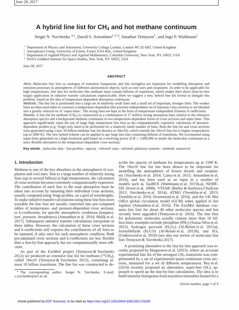
In order to illustrate the applicability of this approximation,in Figure 8 we show the error of the methane continuum atT = 2000 K andP = 10 bar as the difference between twocross sections: (i) obtained using theJ-dependent Voigt-profilemodel by Barton et al. (2017) and (ii) obtained using constantVoigt parameters, relative to the total methane cross sections atthese values ofT andP. The error is within 0.05 % for most ofthe frequency range and not larger than 0.1 %. Another artefactof the histogram method (apart from the limited profile descrip-tion) is the error of the line position within a bin. Therefore, thesmaller the bin, the better the accuracy of the super-line list.

The important advantage of histograms is that they are veryrobust and efficient for computing cross sections thanks to a rel-atively small number of super-lines defined by the density ofthewavenumber grid, which is therefore much smaller (at least formethane) than the number of the original lines. For example,with the 0.01 cm−1 grid spacing, the size of a histogram at agivenT is only 1,200,000 grid points (super-lines) for our linelist coverage (< 12, 000 cm−1), which is much smaller than theoriginal 34 billion lines. Even for the more sophisticated four-grid model suggested by Tennyson et al. (2016) (∆ν = 10−5 cm−1

Article number, page 5 of 9

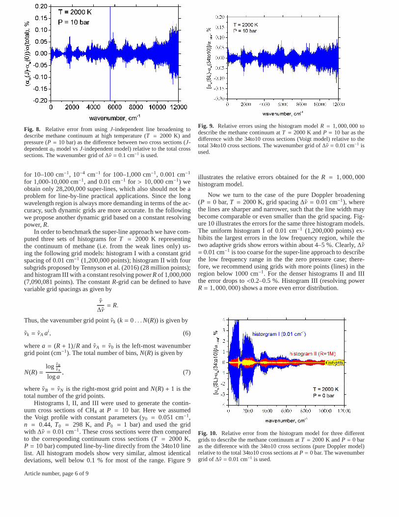
Fig. 8. Relative error from usingJ-independent line broadening todescribe methane continuum at high temperature (T = 2000 K) andpressure (P = 10 bar) as the difference between two cross sections (J-dependenta0 model vsJ-independent model) relative to the total crosssections. The wavenumber grid of∆ν = 0.1 cm−1 is used.

for 10–100 cm−1, 10−4 cm−1 for 100–1,000 cm−1, 0.001 cm−1

for 1,000-10,000 cm−1, and 0.01 cm−1 for > 10, 000 cm−1) weobtain only 28,200,000 super-lines, which also should not be aproblem for line-by-line practical applications. Since the longwavelength region is always more demanding in terms of the ac-curacy, such dynamic grids are more accurate. In the followingwe propose another dynamic grid based on a constant resolvingpower,R.

In order to benchmark the super-line approach we have com-puted three sets of histograms forT = 2000 K representingthe continuum of methane (i.e. from the weak lines only) us-ing the following grid models: histogram I with a constant gridspacing of 0.01 cm−1 (1,200,000 points); histogram II with foursubgrids proposed by Tennyson et al. (2016) (28 million points);and histogram III with a constant resolving powerR of 1,000,000(7,090,081 points). The constantR-grid can be defined to havevariable grid spacings as given by

ν

∆ν= R.

Thus, the vavenumber grid point ˜νk (k = 0 . . .N(R)) is given by

νk = νA ai, (6)

wherea = (R + 1)/R and νA = ν0 is the left-most wavenumbergrid point (cm−1). The total number of bins,N(R) is given by

N(R) =log νB

νA

loga, (7)

whereνB = νN is the right-most grid point andN(R) + 1 is thetotal number of the grid points.

Histograms I, II, and III were used to generate the contin-uum cross sections of CH4 at P = 10 bar. Here we assumedthe Voigt profile with constant parameters (γ0 = 0.051 cm−1,n = 0.44, T0 = 298 K, andP0 = 1 bar) and used the gridwith ∆ν = 0.01 cm−1. These cross sections were then comparedto the corresponding continuum cross sections (T = 2000 K,P = 10 bar) computed line-by-line directly from the 34to10 linelist. All histogram models show very similar, almost identicaldeviations, well below 0.1 % for most of the range. Figure 9

Fig. 9. Relative errors using the histogram modelR = 1,000, 000 todescribe the methane continuum atT = 2000 K andP = 10 bar as thedifference with the 34to10 cross sections (Voigt model) relative to thetotal 34to10 cross sections. The wavenumber grid of∆ν = 0.01 cm−1 isused.

illustrates the relative errors obtained for theR = 1, 000, 000histogram model.

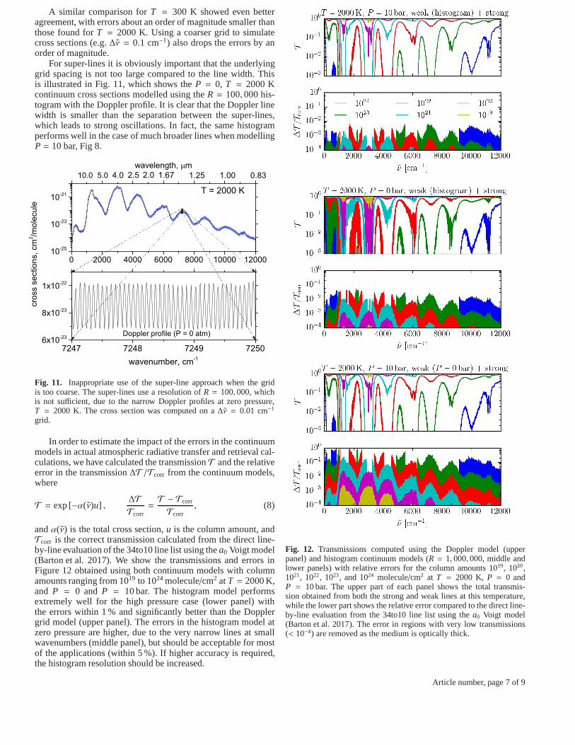
Now we turn to the case of the pure Doppler broadening(P = 0 bar,T = 2000 K, grid spacing∆ν = 0.01 cm−1), wherethe lines are sharper and narrower, such that the line width maybecome comparable or even smaller than the grid spacing. Fig-ure 10 illustrates the errors for the same three histogram models.The uniform histogram I of 0.01 cm−1 (1,200,000 points) ex-hibits the largest errors in the low frequency region, whilethetwo adaptive grids show errors within about 4–5 %. Clearly,∆ν= 0.01 cm−1 is too coarse for the super-line approach to describethe low frequency range in the the zero pressure case; there-fore, we recommend using grids with more points (lines) in theregion below 1000 cm−1. For the denser histograms II and IIIthe error drops to<0.2–0.5 %. Histogram III (resolving powerR = 1, 000, 000) shows a more even error distribution.

Fig. 10. Relative error from the histogram model for three differentgrids to describe the methane continuum atT = 2000 K andP = 0 baras the difference with the 34to10 cross sections (pure Doppler model)relative to the total 34to10 cross sections atP = 0 bar. The wavenumbergrid of ∆ν = 0.01 cm−1 is used.

Article number, page 6 of 9

A similar comparison forT = 300 K showed even betteragreement, with errors about an order of magnitude smaller thanthose found forT = 2000 K. Using a coarser grid to simulatecross sections (e.g.∆ν = 0.1 cm−1) also drops the errors by anorder of magnitude.

For super-lines it is obviously important that the underlyinggrid spacing is not too large compared to the line width. Thisis illustrated in Fig. 11, which shows theP = 0, T = 2000 Kcontinuum cross sections modelled using theR = 100, 000 his-togram with the Doppler profile. It is clear that the Doppler linewidth is smaller than the separation between the super-lines,which leads to strong oscillations. In fact, the same histogramperforms well in the case of much broader lines when modellingP = 10 bar, Fig 8.

0 2000 4000 6000 8000 10000 1200010-25

10-23

10-21

wavelength, m

T = 2000 K

cros

s se

ctio

ns, c

m2 /m

olec

ule

0.831.001.251.672.02.54.05.0 10.0

7247 7248 7249 72506x10-23

8x10-23

1x10-22

wavenumber, cm-1

Doppler profile (P = 0 atm)

Fig. 11. Inappropriate use of the super-line approach when the gridis too coarse. The super-lines use a resolution ofR = 100, 000, whichis not sufficient, due to the narrow Doppler profiles at zero pressure,T = 2000 K. The cross section was computed on a∆ν = 0.01 cm−1

grid.

In order to estimate the impact of the errors in the continuummodels in actual atmospheric radiative transfer and retrieval cal-culations, we have calculated the transmissionT and the relativeerror in the transmission∆T /Tcorr from the continuum models,where

T = exp [−α(ν)u] ,∆T

Tcorr=T − Tcorr

Tcorr, (8)

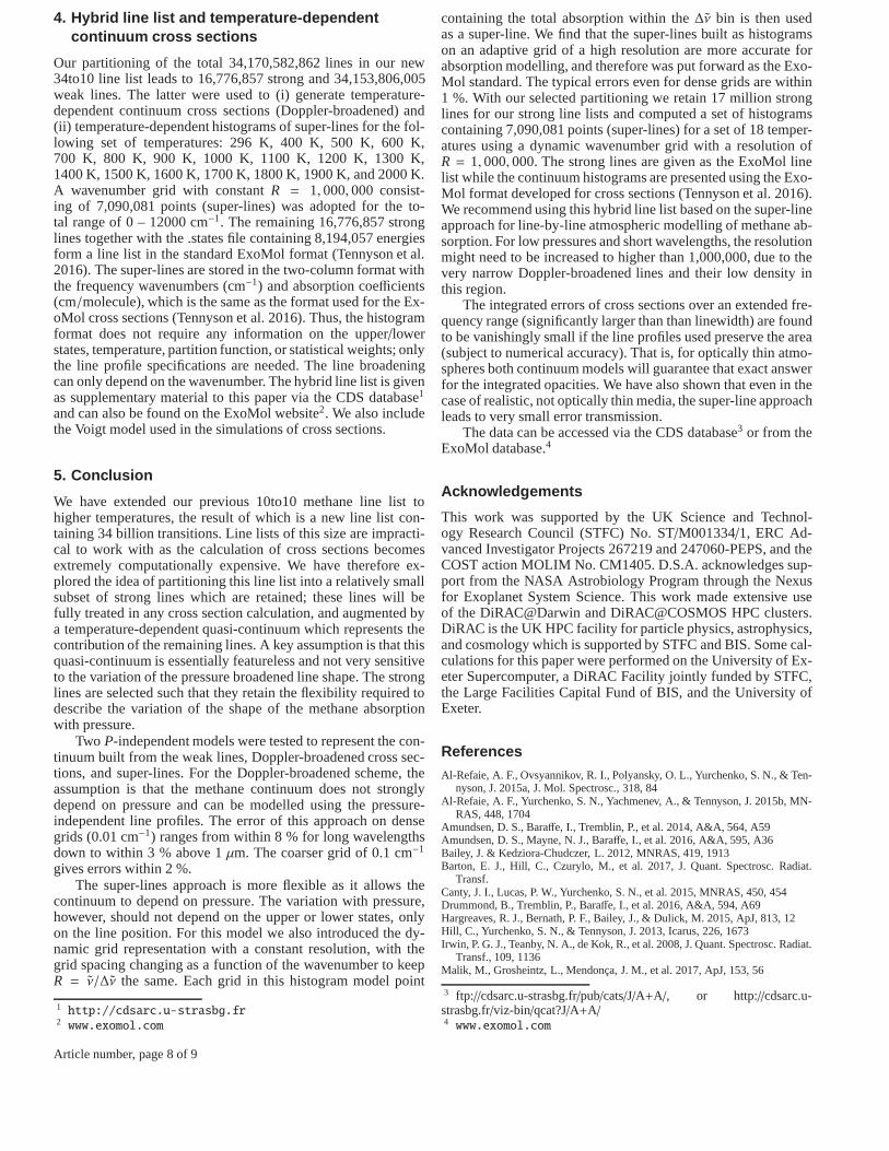
andα(ν) is the total cross section,u is the column amount, andTcorr is the correct transmission calculated from the direct line-by-line evaluation of the 34to10 line list using thea0 Voigt model(Barton et al. 2017). We show the transmissions and errors inFigure 12 obtained using both continuum models with columnamounts ranging from 1019 to 1024 molecule/cm2 atT = 2000 K,and P = 0 and P = 10 bar. The histogram model performsextremely well for the high pressure case (lower panel) withthe errors within 1 % and significantly better than the Dopplergrid model (upper panel). The errors in the histogram model atzero pressure are higher, due to the very narrow lines at smallwavenumbers (middle panel), but should be acceptable for mostof the applications (within 5 %). If higher accuracy is required,the histogram resolution should be increased.

Fig. 12. Transmissions computed using the Doppler model (upperpanel) and histogram continuum models (R = 1, 000, 000, middle andlower panels) with relative errors for the column amounts 1019, 1020,1021, 1022, 1023, and 1024 molecule/cm2 at T = 2000 K, P = 0 andP = 10 bar. The upper part of each panel shows the total transmis-sion obtained from both the strong and weak lines at this temperature,while the lower part shows the relative error compared to thedirect line-by-line evaluation from the 34to10 line list using thea0 Voigt model(Barton et al. 2017). The error in regions with very low transmissions(< 10−4) are removed as the medium is optically thick.

Article number, page 7 of 9

4. Hybrid line list and temperature-dependentcontinuum cross sections

Our partitioning of the total 34,170,582,862 lines in our new34to10 line list leads to 16,776,857 strong and 34,153,806,005weak lines. The latter were used to (i) generate temperature-dependent continuum cross sections (Doppler-broadened) and(ii) temperature-dependent histograms of super-lines forthe fol-lowing set of temperatures: 296 K, 400 K, 500 K, 600 K,700 K, 800 K, 900 K, 1000 K, 1100 K, 1200 K, 1300 K,1400 K, 1500 K, 1600 K, 1700 K, 1800 K, 1900 K, and 2000 K.A wavenumber grid with constantR = 1, 000, 000 consist-ing of 7,090,081 points (super-lines) was adopted for the to-tal range of 0 – 12000 cm−1. The remaining 16,776,857 stronglines together with the .states file containing 8,194,057 energiesform a line list in the standard ExoMol format (Tennyson et al.2016). The super-lines are stored in the two-column format withthe frequency wavenumbers (cm−1) and absorption coefficients(cm/molecule), which is the same as the format used for the Ex-oMol cross sections (Tennyson et al. 2016). Thus, the histogramformat does not require any information on the upper/lowerstates, temperature, partition function, or statistical weights; onlythe line profile specifications are needed. The line broadeningcan only depend on the wavenumber. The hybrid line list is givenas supplementary material to this paper via the CDS database1

and can also be found on the ExoMol website2. We also includethe Voigt model used in the simulations of cross sections.

5. Conclusion

We have extended our previous 10to10 methane line list tohigher temperatures, the result of which is a new line list con-taining 34 billion transitions. Line lists of this size are impracti-cal to work with as the calculation of cross sections becomesextremely computationally expensive. We have therefore ex-plored the idea of partitioning this line list into a relatively smallsubset of strong lines which are retained; these lines will befully treated in any cross section calculation, and augmented bya temperature-dependent quasi-continuum which represents thecontribution of the remaining lines. A key assumption is that thisquasi-continuum is essentially featureless and not very sensitiveto the variation of the pressure broadened line shape. The stronglines are selected such that they retain the flexibility required todescribe the variation of the shape of the methane absorptionwith pressure.

Two P-independent models were tested to represent the con-tinuum built from the weak lines, Doppler-broadened cross sec-tions, and super-lines. For the Doppler-broadened scheme,theassumption is that the methane continuum does not stronglydepend on pressure and can be modelled using the pressure-independent line profiles. The error of this approach on densegrids (0.01 cm−1) ranges from within 8 % for long wavelengthsdown to within 3 % above 1µm. The coarser grid of 0.1 cm−1

gives errors within 2 %.The super-lines approach is more flexible as it allows the

continuum to depend on pressure. The variation with pressure,however, should not depend on the upper or lower states, onlyon the line position. For this model we also introduced the dy-namic grid representation with a constant resolution, withthegrid spacing changing as a function of the wavenumber to keepR = ν/∆ν the same. Each grid in this histogram model point

1 http://cdsarc.u-strasbg.fr2 www.exomol.com

containing the total absorption within the∆ν bin is then usedas a super-line. We find that the super-lines built as histogramson an adaptive grid of a high resolution are more accurate forabsorption modelling, and therefore was put forward as the Exo-Mol standard. The typical errors even for dense grids are within1 %. With our selected partitioning we retain 17 million stronglines for our strong line lists and computed a set of histogramscontaining 7,090,081 points (super-lines) for a set of 18 temper-atures using a dynamic wavenumber grid with a resolution ofR = 1, 000, 000. The strong lines are given as the ExoMol linelist while the continuum histograms are presented using theExo-Mol format developed for cross sections (Tennyson et al. 2016).We recommend using this hybrid line list based on the super-lineapproach for line-by-line atmospheric modelling of methane ab-sorption. For low pressures and short wavelengths, the resolutionmight need to be increased to higher than 1,000,000, due to thevery narrow Doppler-broadened lines and their low density inthis region.

The integrated errors of cross sections over an extended fre-quency range (significantly larger than than linewidth) arefoundto be vanishingly small if the line profiles used preserve thearea(subject to numerical accuracy). That is, for optically thin atmo-spheres both continuum models will guarantee that exact answerfor the integrated opacities. We have also shown that even inthecase of realistic, not optically thin media, the super-lineapproachleads to very small error transmission.

The data can be accessed via the CDS database3 or from theExoMol database.4

Acknowledgements

This work was supported by the UK Science and Technol-ogy Research Council (STFC) No. ST/M001334/1, ERC Ad-vanced Investigator Projects 267219 and 247060-PEPS, and theCOST action MOLIM No. CM1405. D.S.A. acknowledges sup-port from the NASA Astrobiology Program through the Nexusfor Exoplanet System Science. This work made extensive useof the DiRAC@Darwin and DiRAC@COSMOS HPC clusters.DiRAC is the UK HPC facility for particle physics, astrophysics,and cosmology which is supported by STFC and BIS. Some cal-culations for this paper were performed on the University ofEx-eter Supercomputer, a DiRAC Facility jointly funded by STFC,the Large Facilities Capital Fund of BIS, and the UniversityofExeter.

ReferencesAl-Refaie, A. F., Ovsyannikov, R. I., Polyansky, O. L., Yurchenko, S. N., & Ten-

nyson, J. 2015a, J. Mol. Spectrosc., 318, 84Al-Refaie, A. F., Yurchenko, S. N., Yachmenev, A., & Tennyson, J. 2015b, MN-

RAS, 448, 1704Amundsen, D. S., Baraffe, I., Tremblin, P., et al. 2014, A&A, 564, A59Amundsen, D. S., Mayne, N. J., Baraffe, I., et al. 2016, A&A, 595, A36Bailey, J. & Kedziora-Chudczer, L. 2012, MNRAS, 419, 1913Barton, E. J., Hill, C., Czurylo, M., et al. 2017, J. Quant. Spectrosc. Radiat.

Transf.Canty, J. I., Lucas, P. W., Yurchenko, S. N., et al. 2015, MNRAS, 450, 454Drummond, B., Tremblin, P., Baraffe, I., et al. 2016, A&A, 594, A69Hargreaves, R. J., Bernath, P. F., Bailey, J., & Dulick, M. 2015, ApJ, 813, 12Hill, C., Yurchenko, S. N., & Tennyson, J. 2013, Icarus, 226,1673Irwin, P. G. J., Teanby, N. A., de Kok, R., et al. 2008, J. Quant. Spectrosc. Radiat.

Transf., 109, 1136Malik, M., Grosheintz, L., Mendonça, J. M., et al. 2017, ApJ,153, 56

3 ftp://cdsarc.u-strasbg.fr/pub/cats/J/A+A/, or http://cdsarc.u-strasbg.fr/viz-bin/qcat?J/A+A/4 www.exomol.com

Article number, page 8 of 9

Nikitin, A. V., Rey, M., & Tyuterev, V. G. 2017, J. Quant. Spectrosc. Radiat.Transf.,

Rey, M., Nikitin, A. V., Babikov, Y. L., & Tyuterev, V. G. 2016, J. Mol. Spec-trosc., 327, 138

Rey, M., Nikitin, A. V., & Tyuterev, V. G. 2014, ApJ, 789, 2Rothman, L. S., Gordon, I. E., Babikov, Y., et al. 2013, J. Quant. Spectrosc.

Radiat. Transf., 130, 4Sousa-Silva, C., Al-Refaie, A. F., Tennyson, J., & Yurchenko, S. N. 2015, MN-

RAS, 446, 2337Tennyson, J., Bernath, P. F., Campargue, A., et al. 2014, Pure Appl. Chem., 86,

1931Tennyson, J. & Yurchenko, S. N. 2012, MNRAS, 425, 21Tennyson, J. & Yurchenko, S. N. 2017, Mol. Astrophys., 8, 1Tennyson, J., Yurchenko, S. N., Al-Refaie, A. F., et al. 2016, J. Mol. Spectrosc.,

327, 73Tremblin, P., Amundsen, D. S., Chabrier, G., et al. 2016, ApJL, 817, L19Tremblin, P., Amundsen, D. S., Mourier, P., et al. 2015, ApJL, 804, L17Underwood, D. S., Tennyson, J., Yurchenko, S. N., Clausen, S., & Fateev, A.

2016, MNRAS, 462, 4300Waldmann, I. P., Rocchetto, M., Tinetti, G., et al. 2015a, ApJ, 813, 13Waldmann, I. P., Tinetti, G., Barton, E. J., Yurchenko, S. N., & Tennyson, J.

2015b, ApJ, 802, 107Yurchenko, S. N., Al-Refaie, A. F., & Tennyson, J. 2017, Comput. Phys. Com-

mun.Yurchenko, S. N. & Tennyson, J. 2014, MNRAS, 440, 1649Yurchenko, S. N., Tennyson, J., Bailey, J., Hollis, M. D. J.,& Tinetti, G. 2014,

Proc. Nat. Acad. Sci., 111, 9379Yurchenko, S. N., Tennyson, J., Barber, R. J., & Thiel, W. 2013, J. Mol. Spec-

trosc., 291, 69Yurchenko, S. N., Thiel, W., & Jensen, P. 2007, J. Mol. Spectrosc., 245, 126

Article number, page 9 of 9