A discrete-space urban model with environmental amenities

A discrete-space urban model withenvironmental amenities

Liaila Tajibaeva a,*, Robert G. Haight b, Stephen Polasky c

a Department of Economics, Ryerson University, Toronto, ON M5B 2K3, Canadab USDA Forest Service, Northern Research Station, St. Paul, MN 55108, USA

c Department of Applied Economics, University of Minnesota, St. Paul, MN 55108, USA

Received 13 April 2006; received in revised form 22 August 2007; accepted 6 September 2007

Available online 18 September 2007

Abstract

This paper analyzes the effects of providing environmental amenities associated with open space in adiscrete-space urban model and characterizes optimal provision of open space across a metropolitan area.The discrete-space model assumes distinct neighborhoods in which developable land is homogeneouswithin a neighborhood but heterogeneous across neighborhoods. Open space provides environmentalamenities within the neighborhood it is located and may provide amenities in other neighborhoods (amenityspillover). We solve for equilibrium under various assumptions about amenity spillover effects andtransportation costs in both open-city (with in- and out-migration) and closed-city (fixed population)versions of the model. Increasing open space tends to increase equilibrium housing density and price withina neighborhood. In an open-city model, open space provision also increases housing density and price inother neighborhoods if there is an amenity spillover effect. In a closed-city model, housing density andprices in other neighborhoods can decrease if the pull of the local amenity value is stronger than the pushfrom reduced availability of developable land. We use numerical simulation to solve for the optimal patternof open space in two examples: a simple symmetric case and a simulation based on the Twin CitiesMetropolitan Area, Minnesota, USA. With no amenity spillover, it is optimal to provide the same amount ofopen space in all neighborhoods regardless of transportation cost. With amenity spillover effects andrelatively high transportation cost, it is optimal to provide open space in a greenbelt at the edge of the city.With low transportation cost, open space is provided throughout the city with the exception of neighbor-hoods on the periphery of the city, where the majority of the population lives. A greenbelt still occurs but itslocation is inside the city.# 2007 Elsevier B.V. All rights reserved.

Keywords: Open space; Environmental amenities; Discrete urban economics model

www.elsevier.com/locate/ree

Available online at www.sciencedirect.com

Resource and Energy Economics 30 (2008) 170–196

* Corresponding author. Tel.: +1 416 979 5000x7724; fax: +1 416 598 5916.

E-mail address: [email protected] (L. Tajibaeva).

0928-7655/$ – see front matter # 2007 Elsevier B.V. All rights reserved.doi:10.1016/j.reseneeco.2007.09.001

mailto:[email protected]

http://dx.doi.org/10.1016/j.reseneeco.2007.09.001

1. Introduction

Metropolitan areas in the US are experiencing rapid growth and large-scale conversion ofundeveloped to developed land. Many residents are concerned about the resulting loss of openspace and environmental amenities. Some local governments, as well as private land trusts, haveinstituted policies to acquire land or conservation easements to preserve undeveloped land withinor on the fringe of metropolitan areas. From 1996 through 2004, voters approved 1062 of 1373referenda for open space and parks authorizing the use of $26.4 billion (2000 constant dollars) toacquire open space or development rights (Nelson et al., 2007; Trust for Public Land, 2004).

There are at least two important effects of conserving open space in a metropolitan area. First,open space generates amenities that make nearby areas more attractive, thereby changing thespatial pattern of demand for development. Open space designation may result in shifts indemand between different locales within a given metropolitan area, and it may shift overalldemand by encouraging immigration to (or emigration from) the metropolitan area. Second, openspace designation restricts the supply of land available for development. For reasons of bothdemand and supply, the provision of open space affects equilibrium patterns of land prices anddensity of development within a metropolitan area.

We analyze the effect of designating open space on the spatial pattern of residentialdevelopment, population, and property values in a discrete-space urban economics model. Wedivide the city into discrete neighborhoods and assume that developable land is homogeneouswithin a neighborhood but heterogeneous across neighborhoods. Neighborhoods can differ withrespect to the area available for development, the area of open space, access to employmentopportunities, and existing environmental amenities. Provision of open space in a neighborhoodreduces the area available for development and increases environmental amenities. We considercases where an open space amenity only affects the neighborhood in which it is located (localpublic good) and where an amenity affects multiple neighborhoods (amenity spillover). In themodel, landowners choose to rent land to households, the government for open space, or to theagricultural sector. Households maximize their utility by choosing where to live and how much oftheir income to spend on housing versus other goods. The government chooses property tax ratesand the provision of open space given that it must balance its budget.

We analyze equilibrium outcomes for both an open-city model in which population adjusts sothat utility is the same within the metropolitan area as elsewhere, and a closed-city model inwhich population is held constant and utility levels vary. In both open-city and closed-city modelswe show that equilibrium housing density and after-tax land price in a neighborhood tend toincrease with open space provided in that neighborhood. In an open-city model, open spaceprovision increases housing density and price in other neighborhoods as well if there is anamenity spillover effect. In a closed-city model, whether housing density and prices in otherneighborhoods increase or decrease depends on whether the push from reduced availability ofdevelopable land in the neighborhood with increased open space outweighs the pull of the localamenity value in that neighborhood. For an open city, we also show that the incidence of theproperty tax falls solely on landowners and how taxes are raised (e.g., a uniform city-wide tax or aneighborhood-specific tax) does not affect equilibrium outcomes as long as the city boundariesdo not change.

In addition to analyze equilibrium housing densities and land prices for a given pattern of openspace, we formulate and numerically solve the problem of determining the optimal size andlocation of open space using an open-city model. The presence of amenity spillover has a strongeffect on the results. When open space is a local public good that affects only the immediate

L. Tajibaeva et al. / Resource and Energy Economics 30 (2008) 170–196 171

neighborhood, and assuming Cobb–Douglas preferences, it is optimal to provide the sameamount of open space in all neighborhoods. With amenity spillover effects, optimal open spaceprovision differs across neighborhoods. In this case, it is optimal to provide open space in agreenbelt at the edge of the city when transportation cost is relatively high. For low transportationcost, however, open space is provided throughout the city with the exception of neighborhoods onthe periphery of the city. A greenbelt still occurs but its location is inside the city.

Modeling the urban area as discrete neighborhoods allows us to more fully develop theanalysis of open space amenities. Realistic features such as multiple business centers, existingenvironmental amenities, and amenity values of agricultural land are incorporated in a closed-form analytic solution for equilibrium housing and land prices. In addition, these features areeasily incorporated into the open-city optimization model to determine their impact on theoptimal pattern of open space, housing, and land prices. There is also a sense in whichneighborhoods, rather than points in space, are the natural unit of analysis. Data often come inneighborhoods units (e.g., census blocks) and neighborhoods provide an important sense ofidentity within metropolitan areas.

Our discrete-space model contrasts with most urban economics models that utilizecontinuous-space formulations (see Anas et al., 1998; Huriot and Thisse, 2000 for surveys). In themonocentric city model developed by Alonso (1964), Mills (1967), Mills (1972) and Muth(1969), areas close to the central business district (CBD) are more desirable because of lowercommuting cost. These areas have higher land prices and greater housing density. In many urbaneconomics models, locations are identical except for distance to the CBD, i.e., developmentoccurs on a featureless plain. Polinsky and Shavell (1976) include an environmental amenitycharacterized by its distance to the CBD and show how the amenity changes the spatial pattern ofproperty values. Brueckner et al. (1999) include amenities characterized by distance to the CBDto determine the locations of different income classes. In these two papers, the environmentalamenity does not occupy space. In contrast, Mills (1981), Nelson (1985), and Lee and Fujita(1997), analyze the effects of greenbelts that form a ring of open space, which occupy space andare characterized by their distance to the CBD. Lee and Fujita (1997) analyze the optimalplacement of a greenbelt. Franco and Kaffine (2005) analyze optimal placement and size ofpublic goods in a single-dimensional model. Several papers develop two-dimensional urbanmodels with environmental amenities that show the effect of the location, size and shape of openspace on equilibrium housing, land price, and city boundary in an open-city model (Wu andPlantinga, 2003; Wu, 2006; Kovacs and Larson, 2007). With the exception of Lee and Fujita(1997) and Franco and Kaffine (2005), these papers do not analyze the optimal pattern of openspace provision.

A related literature analyzes the optimal allocation of public goods among different locationsadministered by different taxing authorities. Flatters et al. (1974) analyze the provision of localpublic good in two regions where labor can migrate between regions. Because a migrant does notaccount for the fiscal externality of their move, the distribution of the population among regionsis optimal only under very special circumstances. Stiglitz (1977), Stiglitz (1983) and Fujita(1989) also analyze the provision of a local public goods given fiscal effects. Berliant et al. (2006)develop a model where the number and location of facilities that provide congestible local publicgoods are determined endogenously. An important limitation of these models from the standpointof analyzing open space amenities is that public goods do not take up space and therefore do notcompete with housing for land.

Our paper builds on a remarkable paper by Yang and Fujita (1983) that solves for equilibriumhousing density and land prices given the provision of open space and solves for the optimal

L. Tajibaeva et al. / Resource and Energy Economics 30 (2008) 170–196172

pattern of open space in both open and closed-city models. They use a one-dimensionalformulation and show that the optimal density of open space is a uniform proportion of areaindependent of distance from the CBD when environmental amenities are purely local (i.e., noamenity spillover effects). They briefly consider the case with amenity spillover in a one-dimensional discrete-space model with five neighborhoods. In this paper, we extend the discrete-space model of Yang and Fujita (1983) to a two-dimensional formulation with multipleneighborhoods that includes the amount of open space and housing in each neighborhood. Thisexpansion allows us to consider a richer set of examples with more complicated patterns ofoptimal open space provision, preexisting amenities and multiple CBDs, and to explore theeffects of changes in transportation costs and amenity spillovers.

In the next section we describe the basic discrete-space urban model with open space and otheramenities. We define market equilibrium and show how provision of open space in aneighborhood affects housing density and land price within and outside the neighborhood. Wethen define a social planner’s problem to determine the optimal amount and location of openspace and numerically solve the problem for two examples. The first example is a symmetric citywith a single central business district and no preexisting amenities. In this example we show howthe amenity spillover effect and transportation cost affect optimal city size and spatial patterns ofopen space and housing. The second example is based on data from the Twin Cities MetropolitanArea (Minneapolis–St. Paul, MN, USA), and we show how the presence of two CBDs andspatially heterogeneous existing amenities, including amenities associated with agricultural land,affect the optimal size and location of open space.

2. A discrete-space urban model with open space amenities

In this section we present a spatially explicit model of a city with open space and otherenvironmental amenities. We consider both open-city and closed-city variants of the model. In anopen-city model, population is determined endogenously by in- and out-migration. Inequilibrium, city residents are equally well off living in the city as elsewhere and utility levels arefixed. In a closed-city model, population is fixed but utility levels vary. The city consists of a setof discrete neighborhoods, Q, located on an XY coordinate plane. The location of eachneighborhood is expressed by its coordinates (x, y), which is the centroid of the neighborhood. Aneighborhood’s total land area is denoted by lðx; yÞ.

The model specification allows for multiple business centers. This extension of the monocentriccity model is motivated by the observation that the central business district is not the soleemployment center, nor even the dominant employment center, in many cities. There are J businesscenters, where J is a positive integer bounded above by the total number of neighborhoods in thecity. The business centers are dimensionless. The residents of the city choose to commute to thebusiness center that is located closest to their neighborhood of residence. Let d jðx; yÞ ¼dððx$ x jÞ; ðy$ y jÞÞ be the Euclidian distance from neighborhood (x, y) to neighborhood ðx j; y jÞ.We define the commuting distance for people living in neighborhood (x, y) to be

dCðx; yÞ ¼ min fd jðx; yÞgJj¼1:

The commuting cost to work for a resident living in neighborhood (x, y) is denoted by

f ½dCðx; yÞ&;

where f is an increasing function of commuting distance, dCðx; yÞ.


In each neighborhood in the city, land is allocated for residential use and open space. Theproportion of land devoted to open space in the ðx; yÞ neighborhood is denoted by aðx; yÞ. Openspace creates an environmental amenity that contributes to the well-being of city residents. Whenthere is no amenity spillover effect, open space only contributes to well-being of residents in theneighborhood in which it is located (i.e., it is a local public good). However, with spillovereffects, open space contributes to the well-being of residents living in other neighborhoods aswell, with the contribution declining with the distance between the neighborhood of residenceand the neighborhood in which the open space is located. In addition to the amenity from openspace there may also be amenities associated with preexisting features of a neighborhood. Thesepreexisting features vary from natural environmental amenities (e.g., topography, lakes), positiveman-made amenities (e.g., schools, theatres), to negative features or disamenities (e.g., wastesites, smokestacks). Denote the proportion of area covered by a preexisting amenity located inneighborhood ðx; yÞ by zðx; yÞ. Similar to open space amenities, preexisting amenities may beeither a local public good (or local public bad in the case of a disamenity) or have spillover effectsin other neighborhoods.

Land outside of the city is allocated to a non-development use (agriculture). The residents ofthe city may derive an amenity or a disamenity from their proximity to agricultural land. Denotethe proportion of area covered by agricultural land at location ðx; yÞ as gðx; yÞ. Let V represent theset of agricultural districts that might contribute amenity value to some neighborhood in the city.

For simplicity, we assume that all land is owned by absentee landowners. Landowners rentland to city residents for housing. Let pðx; yÞ represent the (pre-tax) residential land rental pricein neighborhood ðx; yÞ. To provide open space in neighborhood ðx; yÞ the city government rentsland from landowners at price pðx; yÞ. Landowners can also rent land to farmers for agriculture.The agricultural rental price is denoted by pgðx; yÞ. The model endogenously determines theboundary of the city. A neighborhood will be included in the city if and only if pðx; yÞ' pgðx; yÞ.

The city government collects property tax tðx; yÞ in order to pay for open space provision. Thegovernment must satisfy a budget constraint that open space expenditure equals property taxrevenue. One version of the budget constraint is that each neighborhood pays for open spaceprovided in the neighborhood, that is

tðx; yÞ pðx; yÞ½1$ aðx; yÞ $ zðx; yÞ&lðx; yÞ ¼ pðx; yÞaðx; yÞlðx; yÞ: (1)

In this case, the neighborhood property tax rate is: tðx; yÞ ¼ aðx; yÞ=ð1$ aðx; yÞ $ zðx; yÞÞ.The budget constraint can also be specified as a city-wide constraint with a uniform property taxrate t:

X

ðx;yÞ2Q

ft pðx; yÞ½1$ aðx; yÞ $ zðx; yÞ&lðx; yÞg ¼X

ðx;yÞ2Q

f pðx; yÞaðx; yÞlðx; yÞg: (2)

In this case, the uniform city-wide property tax rate is: t ¼Pðx;yÞ2Qf pðx; yÞaðx; yÞl

ðx; yÞg=Pðx;yÞ2Qf pðx; yÞ½1$ aðx; yÞ $ zðx; yÞ&lðx; yÞg. One could also write down intermediate

cases to cover situations with multiple taxing zones or independent jurisdictions within themetropolitan area.

We assume that all households have identical income v and identical utility function u inconsumption, housing, and amenities. Given the distribution of open space, the objective of eachhousehold i is to choose a neighborhood of residence ðx; yÞ2Q, an amount of residential landhiðx; yÞ, and consumption good ciðx; yÞ, to maximize utility subject to its budget constraint. Theattractiveness of living in a neighborhood depends upon the commuting costs from the


neighborhood to the nearest employment center and the amenities. We define the amenityfunction for neighborhood ðx; yÞ as

Aðx; yÞ ¼ Aððx; yÞ; faðs; rÞgðs;rÞ2Q; fzðs; rÞgðs;rÞ2Q; fgðs; rÞgðs;rÞ2VÞ; (3)

which in general depends on the pattern of the provision of open space across neighborhoods,faðs; rÞgðs;rÞ2Q, preexisting amenities across neighborhoods, fzðs; rÞgðs;rÞ2Q, and amenities fromagricultural land outside the city, fgðs; rÞgðs;rÞ2V. We assume that the environmental amenityvalue for neighborhood ðx; yÞ is increasing in open space provided within ðx; yÞ:@Aðx; yÞ=@aðx; yÞ> 0, and that the environmental amenity value for neighborhood ðx; yÞ isnon-decreasing in open space in other neighborhoods @Aðx; yÞ=@aðs; rÞ' 0 (strictly increasingwith positive spillover effects). We further assume that ‘‘own-neighborhood’’ amenity effect islarger than the ‘‘cross-neighborhood’’ amenity effect for an increase in open space:@Aðx; yÞ=@aðx; yÞ> @Aðs; rÞ=@aðx; yÞ for all ðx; yÞ2Q, ðs; rÞ2Q, s 6¼ x, or r 6¼ y. Preexistingamenities and agricultural amenities can have positive or negative effects. A household i residingin neighborhood ðx; yÞ solves the following problem:

max ciðx;yÞ;hiðx;yÞu½ciðx; yÞ; hiðx; yÞ;Aðx; yÞ& (4a)

such that:

ciðx; yÞ þ ptðx; yÞhiðx; yÞ þ f ½dCðx; yÞ& ) v (4b)

ciðx; yÞ' 0; hiðx; yÞ' 0; (4c)

where u is a continuous, quasi-concave utility function increasing in each argument andptðx; yÞ ¼ ½1þ tðx; yÞ& pðx; yÞ is the after-tax residential land rental price. Note that tðx; yÞ ¼t in the case of a uniform city-wide tax.

3. Market equilibrium

We formulate a market equilibrium for the households, landowners, and the government. Letnðx; yÞ be the number of households living in neighborhood ðx; yÞ. Let N be a fixed population sizeof the city in a closed-city model (N endogenously determined in an open-city model) and let u be afixed reservation utility in an open-city model (u endogenously determined in a closed-city model).

3.1. Definition

Given an open space allocation, preexisting amenities, property taxes, and agricultural rentalprices, faðx; yÞ; zðx; yÞ; tðx; yÞ; pgðx; yÞgðx;yÞ2Q

, location of business centers fbðx j; y jÞgJj¼1, a

uniform utility level u in an open city, and a population size N in a closed city, a marketequilibrium is defined as allocation ffciðx; yÞ; hiðx; yÞgnðx;yÞ

i¼1 ; nðx; yÞgðx;yÞ2Q and a price systemf ptðx; yÞg, such that:1. Households maximize utility in each location: allocation fciðx; yÞ; hiðx; yÞgnðx;yÞ

i¼1 for allðx; yÞ2Q maximizes utility function (Eq. (4a)) subject to budget constraint (Eq. (4b)) andnon-negativity conditions (4c).

2. No arbitrage across locations holds for all neighborhoods ðx; yÞ2Q:

u½ciðx; yÞ; hiðx; yÞ;Aðx; yÞ& ¼ u in an open city (5a)


and

u½ciðx; yÞ; hiðx; yÞ;Aðx; yÞ& ¼ u½ciðs; rÞ; hiðs; rÞ;Aðs; rÞ&

for all ðs; rÞ2Q in a closed city:(5b)

3. Determination of city boundaries satisfies:

pðx; yÞ' pgðx; yÞ for each neighborhood ðx; yÞ2Q and pðx; yÞ< pgðx; yÞ

for any location ðx; yÞ =2Q:(6)

4. The government balances its budget: for each neighborhood ðx; yÞ2Q with the neighborhoodtax (Eq. (1)), or with the city-wide tax (Eq. (2)).

5. The land market clears for all neighborhoods ðx; yÞ2Q (i.e., residential area, plus open spacearea, plus preexisting amenities area equals total neighborhood area):

nðx; yÞhiðx; yÞ þ aðx; yÞlðx; yÞ þ zðx; yÞlðx; yÞ ¼ lðx; yÞ: (7)6. Total population satisfies:

X

ðx;yÞ2Q

nðx; yÞ ¼ N in an open city; (8a)

X

ðx;yÞ2Q

nðx; yÞ ¼ N in a closed city and

nðx; yÞ' 0 for all neighborhoods ðx; yÞ2Q: (8b)

3.2. Equilibrium results

The market equilibrium conditions along with the assumptions of the model can be used todemonstrate several general results of the effect of open space on land rental prices anddevelopment patterns. For the closed-city model, we also need an additional condition in order toprove the first proposition.

Condition 1. For any two neighborhoods ðx; yÞ and ðs; rÞ such that x 6¼ s or y 6¼ r, whereuðciðx; yÞ; hiðx; yÞ;Aðx; yÞÞ ¼ uðciðs; rÞ; hiðs; rÞ;Aðs; rÞÞ, then ð@uðciðx; yÞ; hiðx; yÞ;Aðx; yÞÞ=@Aðx; yÞÞð@Aðx; yÞ=@aðx; yÞÞ> ð@uðciðs; rÞ; hiðs; rÞ;Aðs; rÞÞ=@Aðs; rÞÞð@Aðs; rÞ=@aðx; yÞÞ.

Condition 1 will be satisfied in most but not all circumstances. Because the ‘‘own-neighborhood’’ amenity effect is larger than the ‘‘cross-neighborhood’’ amenity effect for anincrease in open space: @Aðx; yÞ=@aðx; yÞ> @Aðs; rÞ=@aðx; yÞ, Condition 1 will hold unless themarginal utility of amenities is much higher in other neighborhoods. Condition 1 may be violatedif there is decreasing marginal utility of amenities and other neighborhoods begin with far feweramenities.

Proposition 1. Assuming the consumption good and housing are normal goods, an increase inopen space in neighborhood ðx; yÞ will increase the after-tax rental price of land in theneighborhood, ptðx; yÞ, and increase household density in the developed area of the neighbor-hood, nðx; yÞ=ðlðx; yÞð1$ aðx; yÞ $ zðx; yÞÞÞ, for the open-city model and, assuming Condition 1,for the closed-city model.


The proofs of this proposition and all following propositions are given in Appendix A.An increase in open space in a neighborhood increases the amenity value of that

neighborhood, leading to an increase in utility of living in the neighborhood other thingsconstant. In the open-city model, the increase in utility will attract people to the neighborhood,bidding up price and increasing housing density. In the closed-city model, an increase in openspace will cause a greater increase in utility in that neighborhood than in others (Condition 1)thereby attracting people to the neighborhood thereby bidding up price and increasing housingdensity.

Proposition 1 shows that an increase in open space increases the price that residents in thatneighborhood pay for land, ptðx; yÞ, and decreases the amount of housing consumed perhousehold so that housing density in the developed area increases (assuming Condition 1 for aclosed-city model). However, because increasing open space increases taxes and takes some landout of development, the overall effect of an increase in open space on neighborhood populationand the total value of developed land in the neighborhood is ambiguous. Often, it is these type ofaggregate effects that are of greatest interest. For example, municipal leaders might be interestedin knowing whether the tax base would increase or decrease with an increase in open space. If thepull of the open space amenity on demand is strong enough, both population and the value ofdeveloped land within the neighborhood will increase with an increase in open space. However, ifthe supply side push from lowering the amount of developable land in the neighborhood isstronger, neighborhood population and the total value of developed land will fall with an increasein open space. Similarly, the pre-tax rental price that landowners receive may increase ordecrease with an increase in open space.

In the open-city model, we are able to derive several analytical results using the generalframework, including the effect of increased open space in one neighborhood on prices andhousing density in other neighborhoods.

Proposition 2. Assuming the consumption good and housing are normal goods, an increase inopen space in neighborhood ðx; yÞ will result in an increase in the after-tax rental price of land inother neighborhoods, ptðs; rÞ, and an increase in household density in the developed area ofother neighborhoods, nðs; rÞ=ðlðs; rÞð1$ aðs; rÞ $ zðs; rÞÞÞ, for the open-city model when thereare positive spillover effects. There will be no effect on after-tax rental price of land or householddensity in the open-city model when spillover effects are zero.

In the case of a closed city with a fixed population, an increase in open space in oneneighborhood can either increase or decrease the after-tax rental price of land and density in otherneighborhoods. Price and density in other neighborhoods tends to increase because open spaceprovision reduces developable land, which increases the pressure on remaining developable landin all neighborhoods. This effect in other neighborhoods is reinforced when there are strongamenity spillovers. On the other hand, if there are strong local amenity effects, this will tend tocreate a pull toward the neighborhood with open space, thereby reducing demand for otherneighborhoods, which may result in lower prices and lower density.

Proposition 3. In an open-city model, how open space is paid for, whether each neighborhoodpays for its own open space or there is a city-wide property tax, affects pre-tax equilibriumrental prices of land, pðx; yÞ but does not affect after-tax rental prices, ptðx; yÞ, or decisions byhouseholds in equilibrium, ciðx; yÞ; hiðx; yÞ; nðx; yÞ, for any neighborhood that remains inthe city.


As long as the best use of the land in neighborhood ðx; yÞ remains urban use rather thanagriculture, the landlord will absorb the increased property tax leaving the post-tax rental price ofland constant. Post-tax land rental price, ptðx; yÞ, is fixed because the mobility of residents forcesutility levels to u. Pre-tax land rental price, pðx; yÞ, is pure rents to landowners. As long aspðx; yÞ' pgðx; yÞ, landowners will continue to rent to households (and the city government foropen space). In this case, a property tax has no distortionary impacts. This case provides an examplewhere the land tax promoted by George (1984) is the preferred form of taxation as all incidence fallson landowners who supply land inelastically, resulting only in redistributive not efficiencyconsequences from increased taxation. Only when pðx; yÞ< pgðx; yÞwill landowners remove landfrom urban use and instead rent land to farmers. At this point increased property taxes are no longerneutral but will result in a smaller city with fewer neighborhoods and lower population.

3.3. Analytic solution

To make further progress, it is necessary to specify a functional form. With specific functionalforms it is possible to obtain a closed-form analytic solution for equilibrium. Here we assume thatthe utility function is Cobb–Douglas:

uðciðx; yÞ; hiðx; yÞ;Aðx; yÞÞ ¼ a ln ðciðx; yÞÞ þ b ln ðhiðx; yÞÞ þ g ln Aðx; yÞ: (9)

For each ðx; yÞ2Q a household living in the neighborhood chooses consumption good, ciðx; yÞ, andhousing, hiðx; yÞ, to maximize its utility function (Eq. (9)) subject to budget constraint (Eq. (4b))and non-negativity conditions (4c). The Lagrangian for this utility maximization problem is

L ¼ a ln ciðx; yÞ þ b ln hiðx; yÞ þ g ln Aðx; yÞ

þ lðv$ ciðx; yÞ $ ptðx; yÞhiðx; yÞ $ f ½dCðx; yÞ&Þ:The objective function is strictly increasing in both c and h and the lim h! 0uc ¼1 andlim n! 0uh ¼1. The objective function is also concave and subject to linear constraints.Therefore, there exists a unique interior solution to the household’s maximization problem.The following first-order conditions are necessary and sufficient for this solution:

@L@ciðx; yÞ

¼ a

ciðx; yÞ$ l ¼ 0;

@L@hiðx; yÞ

¼ b

hiðx; yÞ$ l ptðx; yÞ ¼ 0;

@L@l¼ v$ ciðx; yÞ $ ptðx; yÞhiðx; yÞ $ f ½dCðx; yÞ& ¼ 0:

The first-order conditions are solved for the household demand functions for the consumptiongood and housing:

ciðx; yÞ ¼a

aþ bðv$ f ½dCðx; yÞ&Þ; (10a)

hiðx; yÞ ¼b

aþ b

!v$ f ½dCðx; yÞ&

ptðx; yÞ

": (10b)

3.3.1. Open cityFor an open city, we use the household demand (Eqs. (10a) and (10b)), the total land area

constraints (Eq. (7)), the no arbitrage condition across locations (5a), to find the equilibrium


allocation, ffciðx; yÞ; hiðx; yÞgnðx;yÞi¼1 ; nðx; yÞgðx;yÞ2Q, and prices, f ptðx; yÞgðx;yÞ2Q (see

Appendix B for the full derivation of the solution):

ciðx; yÞ ¼a


hiðx; yÞ ¼!

aþ b

a

"a=beu=b

ðv$ f ½dCðx; yÞ&Þa=bAðx; yÞg=b; (11b)

ptðx; yÞ ¼ max

#aa=bb

ðaþ bÞðaþbÞ=b eu=bðv$ f ½dCðx; yÞ&ÞðaþbÞ=bAðx; yÞg=b; pgðx; yÞ

$;

(11c)

nðx; yÞ ¼!

a

aþ b

"a=b

e$u=b½1$ aðx; yÞ $ zðx; yÞ&lðx; yÞðv$ f ½dCðx; yÞ&Þa=bAðx; yÞg=b:

(11d)

3.3.2. Closed cityFor a closed city, we use the household demand (Eqs. (10a) and (10b)), the total land area

constraints (Eq. (7)), the no arbitrage condition across locations (5b), and the fact that totalpopulation is fixed at N (Eq. (8b)), to find the equilibrium allocation,ffciðx; yÞ; hiðx; yÞgnðx;yÞ

i¼1 ; nðx; yÞgðx;yÞ2Q, and prices, f ptðx; yÞgðx;yÞ2Q (see Appendix C for thefull derivation of the solution):

ciðx; yÞ ¼a


hiðx; yÞ ¼

Pðs;rÞ2Q

#ð1$ aðx; yÞ $ zðx; yÞÞlðx; yÞðv$ f ½dCðs; rÞ&Þa=bAðs; rÞg=b

$

Nðv$ f ½dCðx; yÞ&Þa=bAðx; yÞg=b;

(12b)

ptðx; yÞ ¼ max

(bNðv$ f ½dCðx; yÞ&ÞðaþbÞ=bAðx; yÞg=b

ðaþ bÞPðs;rÞ2Qfð1$ aðx; yÞ $ zðx; yÞÞlðx; yÞ

ðv$ f ½dCðs; rÞ&Þa=bAðs; rÞg=bg

; pg

)

; (12c)

nðx; yÞ ¼ Nð1$ aðx; yÞ $ zðx; yÞÞlðx; yÞðv$ f ½dCðx; yÞ&Þa=bAðx; yÞg=bPðs;rÞ2Qfð1$ aðx; yÞ $ zðx; yÞÞlðx; yÞðv$ f ½dCðs; rÞ&Þa=bAðs; rÞg=bg

: (12d)

With this solution it is straight-forward to demonstrate the effect of adding open space in a givenneighborhood on the pattern of development and land prices in the urban area. Another advantageof this model is that it is easy to add a variety of amenities (lakes, wetlands, hills) anddisamenities (waste sites, smokestacks) in addition to open space amenities.

Given the open space distribution faðx; yÞgðx;yÞ2Q, the preexisting amenities fzðx; yÞgðx;yÞ2Q,and the business centers fbðx j; y jÞg

Jj¼1, we use the housing price ptðx; yÞ and demand hiðx; yÞ

equations to solve for the fringe neighborhoods using condition (6) from the definition of theequilibrium.


4. Optimal provision of open space

In the analysis of equilibrium in the previous section, the allocation of open space acrossneighborhoods is given. Here we tackle the problem of optimal provision of open space whenthere are amenity spillover effects among neighborhoods. This problem has been analyzedpreviously for a restricted single-dimensional example with five neighborhoods in Yang andFujita (1983). As the algebra gets complicated with amenity spillover, we restrict our analysis tothe case of the open-city model. In solving for the optimal allocation, it is easier to work with thebid-rent function rather than the direct demand functions as has been done above. Assuming thatthe utility function is concave in ciðx; yÞ, hiðx; yÞ, and Aðx; yÞ, the household utility maximizationproblem can be restated as a bid-rent function maximization problem. That is, in order for ahousehold to maintain a utility level u, what is the maximum price that this household is willingto pay to reside in some neighborhood ðx; yÞ? This problem is as follows:

max ciðx;yÞv$ ciðx; yÞ $ f ½dCðx; yÞ&

hiðx; yÞsuch that:

u½ciðx; yÞ; hiðx; yÞ;Aðx; yÞ& ' u; ciðx; yÞ' 0:

The solution of this problem is the bid-rent function:

v$ ciðhiðx; yÞ;Aðx; yÞ; uÞ $ f ½dCðx; yÞ&hiðx; yÞ

;

where ciðhiðx; yÞ;Aðx; yÞ; uÞ is the inverse function of u½ciðx; yÞ; hiðx; yÞ;Aðx; yÞ& ¼ u. Given thisbid function, the optimal allocation, ffh*i ðx; yÞg

n*ðx;yÞi¼1 ; n*ðx; yÞ; a*ðx; yÞgðx;yÞ2Q, solves the fol-

lowing problem:

max fhiðx;yÞ;nðx;yÞ;aðx;yÞgðx;yÞ2Q

X

ðx;yÞ2Q

#!v$ ciðhiðx; yÞ;Aðx; yÞ; uÞ $ f ½dCðx; yÞ&

hiðx; yÞ$ pgðx; yÞ

"

+ nðx; yÞhiðx; yÞ $ aðx; yÞlðx; yÞ pgðx; yÞ$

(13a)

subject to

nðx; yÞhiðx; yÞ þ aðx; yÞlðx; yÞ þ zðx; yÞlðx; yÞ ) lðx; yÞ for all ðx; yÞ2Q

nðx; yÞ' 0; hiðx; yÞ' 0; 1' aðx; yÞ' 0 for all ðx; yÞ2Q;(13b)

where the objective function is the bid-rent function net of the opportunity cost of an alternativeland use pattern. To simplify the optimization problem, first observe that the total land constraintwill hold with equality because household’s preferences are strictly increasing in housing, so wecan substitute ð1$ aðx; yÞ $ zðx; yÞÞlðx; yÞ from Eq. (13b) for nðx; yÞhiðx; yÞ in the objectivefunction (13a). Second, observe that after the substitution the optimal housing allocation as afunction of amenities, distance, and utility level, can be obtained by solving

max hiðx;yÞv$ ciðhiðx; yÞ;Aðx; yÞ; uÞ $ f ½dCðx; yÞ&

hiðx; yÞ:


If we use the utility function specification given in Eq. (9), then the solution of this maximizationproblem in housing is

hiðx; yÞ ¼!

aþ b

a

"a=b eu=b

ðv$ f ½dCðx; yÞ&Þa=bAðx; yÞg=b:

With these two observations, the utility function, and rearranging the terms, the optimizationproblem can be restated as follows:

max faðx;yÞgðx;yÞ2Q

X

ðx;yÞ2Q

aa=bb

ðaþbÞðaþbÞ=b eu=bðv$ f ½dCðx; yÞ&ÞðaþbÞ=bAðx; yÞg=bð1$ aðx; yÞ

$zðx; yÞÞlðx; yÞ $ pgðx; yÞlðx; yÞ

0

BB@

1

CCA

subject to : aðx; yÞ2 ½0; 1& for all ðx; yÞ2Q:

The solution is the optimal allocation of open space fa*ðx; yÞgðx;yÞ2Q. Using this optimalallocation of open space we solve for the optimal allocations of housing ffh*i ðx; yÞg

n*ðx;yÞi¼1 gðx;yÞ2Q,

and density fn*ðx; yÞgðx;yÞ2Q.Similar to the results in Yang and Fujita (1983), given the optimal allocation of open

space, fa*ðx; yÞgðx;yÞ2Q, and the same level of utility and preexisting amenities, the marketequilibrium allocation ffciðx; yÞ; hiðx; yÞgnðx;yÞ

i¼1 ; nðx; yÞgðx;yÞ2Q, and the optimal allocation,ffc*i ðx; yÞ; h*i ðx; yÞg

n*ðx;yÞi¼1 ; n*ðx; yÞgðx;yÞ2Q, are identical.

Unlike the equilibrium solution shown above, the optimal solution with amenity spilloversdoes not have a closed-form analytical solution. In the next section, we solve for the optimalspatial allocation of open space using numerical simulation.

5. Simulation results

In this section, we determine the optimal spatial pattern of open space, equilibrium populationand land rents for an open-city model using numerical simulation for two examples. The firstexample is a symmetric city with a single central business district and no preexisting amenities.This example is relatively transparent and we use it to highlight the effects of changes in amenityspillovers and transportation costs on the optimal spatial pattern of open space, population, andequilibrium land rents. The second example is based on data from the Twin Cities MetropolitanArea (Minneapolis–St. Paul, MN, USA). The Twin Cities have two downtowns, one inMinneapolis and another in St. Paul, and a large number of existing lakes and parks. Thisexample is used to explore potentially asymmetric solutions as well as to demonstrate how such amodel might be parameterized and applied to a metropolitan area with multiple employmentcenters and a large variety of preexisting features such as commercial development, parks, andnatural landscapes.

5.1. Symmetric example

In this first example, we optimize open space allocation for a symmetric city with a centralbusiness district (CBD) located at the origin ð0; 0Þ on a 25+ 25 grid of square neighborhoods.Each neighborhood has unit area and has its center represented by its ðx; yÞ coordinates. We use alinear transportation cost function: f ½dCðx; yÞ& ¼ sdCðx; yÞ. We experimented with an alternativespecification of the transportation cost function, specifically an exponential cost function


f ½dCðx; yÞ& ¼ exp ½sdCðx; yÞ& (Lucas and Rossi-Hansberg, 2002). We obtained qualitativelysimilar results with both transportation cost functions and so only report results using the linearcost function here. In general, a variety of transportation cost forms can be used because themodel is quite flexible. We specify the amenity function (Eq. (3)) for neighborhood ðx; yÞ, Aðx; yÞ,to be

Aðx; yÞ ¼X

ðs;rÞ2Q

½daaðs; rÞ þ dzzðs; rÞ&lðs; rÞ exp ½$fdðx$ s; y$ rÞ&

þX

ðs;rÞ2V

½dzzðs; rÞ þ dggðs; rÞ&lðs; rÞ exp ½$fdðx$ s; y$ rÞ&; (14)

where aðs; rÞlðs; rÞ is the area of open space in neighborhood ðs; rÞ, zðs; rÞlðs; rÞ the area ofpreexisting amenity in neighborhood ðs; rÞ, gðs; rÞlðs; rÞ the area of agricultural land inneighborhood ðs; rÞ, and da, dz, dg, are the amenity value weights for open space, preexistingamenities, and agricultural land, respectively, with da > 0. The values of dz and dg may be eitherpositive (amenity), zero, or negative (disamenity). f is the parameter that measures the effect of

distance to an amenity, and dðx$ s; y$ rÞ ¼ffiffiffiffiffiffiffiffiffiffiffiffiffiffiffiffiffiffiffiffiffiffiffiffiffiffiffiffiffiffiffiffiffiffiffiffiffiðx$ sÞ2 þ ðy$ rÞ2

qis the distance between

neighborhoods ðx; yÞ and ðs; rÞ.The parameter values used in the simulation are given in Table 1. We vary the amenity

spillover effect and the transportation cost across different simulations. Because the parametervalues for a given simulation are homogeneous across neighborhoods, we assume that theoptimal spatial pattern of open space, population, and land rents is symmetric around the CBD.For each set of parameter values, we determine the optimal pattern of open space for cities ofincreasing radius until the equilibrium land rent on the perimeter is equal to the price ofagricultural land. The optimization problem is formulated and solved using GAMS and thenonlinear solver CONOPT. The algorithm found the same identical solution for a given problemeven when we initiated the algorithm at different starting points adding to our confidence that wehave indeed found a unique optimal solution.

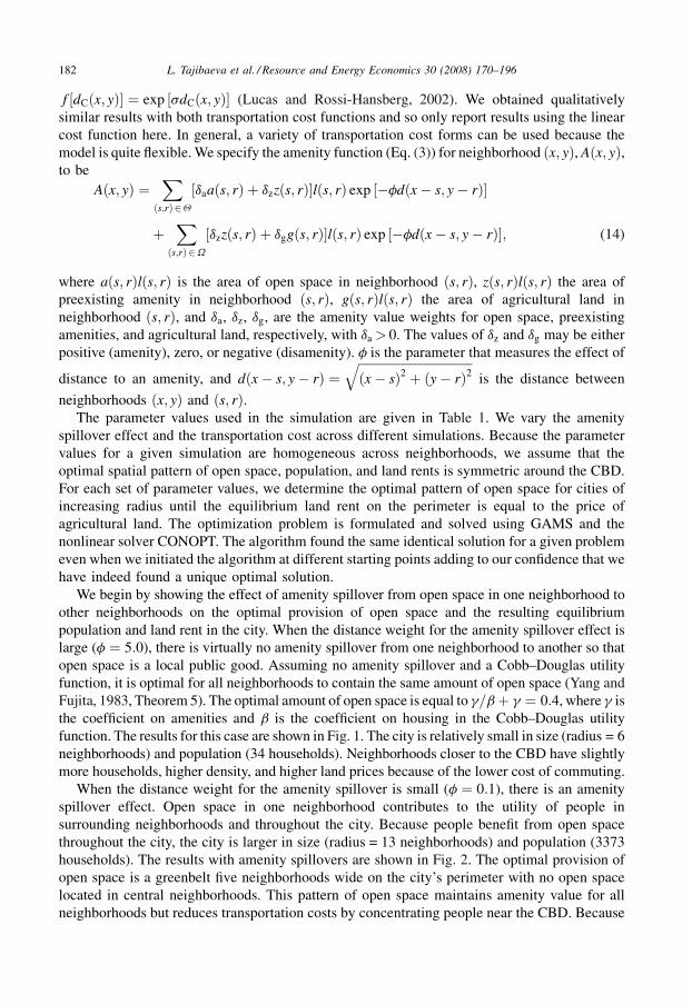
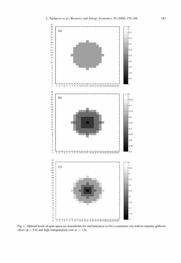
We begin by showing the effect of amenity spillover from open space in one neighborhood toother neighborhoods on the optimal provision of open space and the resulting equilibriumpopulation and land rent in the city. When the distance weight for the amenity spillover effect islarge (f ¼ 5:0), there is virtually no amenity spillover from one neighborhood to another so thatopen space is a local public good. Assuming no amenity spillover and a Cobb–Douglas utilityfunction, it is optimal for all neighborhoods to contain the same amount of open space (Yang andFujita, 1983, Theorem 5). The optimal amount of open space is equal to g=bþ g ¼ 0:4, where g isthe coefficient on amenities and b is the coefficient on housing in the Cobb–Douglas utilityfunction. The results for this case are shown in Fig. 1. The city is relatively small in size (radius = 6neighborhoods) and population (34 households). Neighborhoods closer to the CBD have slightlymore households, higher density, and higher land prices because of the lower cost of commuting.

When the distance weight for the amenity spillover is small (f ¼ 0:1), there is an amenityspillover effect. Open space in one neighborhood contributes to the utility of people insurrounding neighborhoods and throughout the city. Because people benefit from open spacethroughout the city, the city is larger in size (radius = 13 neighborhoods) and population (3373households). The results with amenity spillovers are shown in Fig. 2. The optimal provision ofopen space is a greenbelt five neighborhoods wide on the city’s perimeter with no open spacelocated in central neighborhoods. This pattern of open space maintains amenity value for allneighborhoods but reduces transportation costs by concentrating people near the CBD. Because



Fig. 1. Optimal levels of open space (a), households (b), and land price (c) for a symmetric city with no amenity spillovereffect (f ¼ 5:0) and high transportation cost (s ¼ 1:0).


Fig. 2. Optimal levels of open space (a), households (b), and land price (c) for a symmetric city with amenity spillover

effect (f ¼ 0:1) and high transportation cost (s ¼ 1:0).

the only major difference in locations is related to commuting costs, land prices are very highnear the CBD and decrease rapidly toward the city’s perimeter.

With no amenity spillover effect (f ¼ 5:0), the optimal provision of open space is the sameacross all neighborhoods and is not affected by changes in transportation cost. With an amenityspillover effect (f ¼ 0:1), transportation cost has a big impact on optimal provision of open spaceand on city size. When transportation cost per unit distance (s) is reduced from 1.0 to 0.01, theradius of the city increases by two orders of magnitude to about 1300 neighborhoods for a valueof agricultural land of pg ¼ 1:0. With over 5 million neighborhoods, the optimization problemexceeded the limits of our software. Therefore, we limited the city to a radius of 13neighborhoods and computed optimal open space and population within this city size constraint.

With low transportation cost and a limit on the radius of the city, open space is locatedthroughout the city except in perimeter neighborhoods and a small set of neighborhoods in thecenter of the city (Fig. 3). On the border of the city, there is a densely populated belt without openspace and next to this, inside the city, there is a ring of neighborhoods that have a higherproportion of open space than neighborhoods closer to the CBD giving the impression of agreenbelt. Both the populated belt and the greenbelt are small (i.e., only a few neighborhoods inwidth). Further inside the city, the distribution of open space is relatively homogeneous exceptfor a few neighborhoods surrounding the CBD. Total population (8299) is more than twice thenumber of households in a city with higher transportation cost, and more than half the populationis concentrated in the ring three neighborhoods wide on the city’s perimeter.

This pattern of housing and open space results from the combined effects of low transportationcost, amenity spillover, and limited city size. Within a city of predefined size, transportation costsare almost negligible: moving one neighborhood further outside the city costs only 0.07% ofincome. On the other hand, providing open space on the perimeter of the city carries considerableopportunity cost because almost half of the spillover benefits are wasted. Therefore, the optimalpattern is to provide more open space in a greenbelt close to the city’s border and to move peopleto the neighborhoods outside this greenbelt on the city’s perimeter. Further inside the city, thedistribution of housing and open space is relatively homogeneous because low transportation costblunts the advantage of living close to the CBD.

We conducted sensitivity analysis with regard to the simulated size of the city. As the radius ofthe city is increased, both belts on the perimeter of the city (the outer ring without open space andthe greenbelt) move outward but remain of similar width. Although we did not compute theoptimal provision of open space in a city with endogenous boundaries where pg ¼ 1:0, wespeculate that it would have the same pattern as the city shown in Fig. 3.

5.2. Twin Cities simulation results

In this section, we demonstrate the flexibility of the discrete-space open-city optimizationmodel by applying it to a case with two business centers and asymmetric distributions of existingamenities and development using data for the Twin Cities Metropolitan Region, Minnesota,USA. The study area is 14,300 km2 and includes the cities of Minneapolis and St. Paul andsurrounding area (Fig. 4). We divided the study area into a 13+ 11 grid of 100 km2 squareneighborhoods, each centered around its ðx; yÞ coordinates with the neighborhood in the lowerleft corner labeled (1, 1). Two business centers representing downtown Minneapolis anddowntown St. Paul are located in neighborhoods (6, 6) and (8, 6), respectively. For eachneighborhood, we calculated the proportions of the neighborhood in existing commercialdevelopment, parks and water (Fig. 5) using the 2000 Generalized Land Use data set for the



Fig. 3. Optimal levels of open space (a), households (b), and land price (c) for a symmetric city with amenity spillover

effect (f ¼ 0:1) and low transportation cost (s ¼ 0:01).


Fig. 4. The Twin Cities study area.

Fig. 5. Proportions of 100 km2 neighborhoods currently covered by parks (a), lakes (b), commercial development (c), and

‘‘undeveloped’’ land (total land minus parks, lakes, and commercial development) (d) in the Twin Cities study area.

seven-county Twin Cites Metropolitan Area (Metropolitan Council, 2007). Parks and waterfeatures (lakes, rivers) are treated as amenities. Some of the eastern neighborhoods in our gridspill into an area outside of the Twin Cities Metropolitan Area data. For the purposes of thesimulation we assumed that these neighborhoods are undeveloped. Proportions of commercialdevelopment are greatest near the central business districts. Most neighborhoods have less than10% of their area in amenities. The neighborhoods with more amenities are located around LakeMinnetonka (4, 6), Forest Lake (9, 10), and Spring Lake along the Mississippi River (9, 4). Weassumed that existing commercial development and amenities were fixed at their current levelsand defined ‘undeveloped’ land as total land minus the area of existing parks, lakes, andcommercial development. We then determined the optimal amount of open space, populationlevel, and equilibrium land rent for developable land in each neighborhood.

The parameter values used in the open-city optimization model are given in Table 2. Weassumed the same share parameters ða;b; gÞ in the utility function as in the symmetric example.We used annual household income of $40,915 for Minneapolis–St. Paul in 2004 (Bureau ofEconomic Analysis, 2007). We set the reservation utility level so that the Twin Cities would growfrom its current size (continuing a pattern of growth in recent decades). We assumed the price ofagricultural land to be $4200 per ha ($1700 per acre). Annual transportation cost for commuting


Table 1Parameter values used in the symmetric simulations

Parameter description Parameter value

Consumption good share (a) 0.5

Housing share (b) 0.3Amenities share (g) 0.2

Income (v) 15

Utility level in an open city (u) 1.0

Price of agricultural land ( pg) 1.0

Transportation cost (s) (high and low cost) 1.0 and 0.01

Distance effect on amenity (f) (without and with spillover) 5.0 and 0.1

Amenity value for a unit of open space (da) 1

Amenity value for a unit of preexisting features (dz) 1Amenity value for a unit of agricultural land (dg) 0

Table 2Parameter values used in the twin cities simulation

Parameter description Parameter value

Consumption good share (a) 0.5

Housing share (b) 0.3Amenities share (g) 0.2

Income (v) $1000 per year 40.9

Utility level in an open city (u) 3.0Price of agricultural land ( pg) $1000 per ha 4.2

Transportation cost (s) $1000 per km per year 0.331

Distance effect on amenity (f) 0.1

Amenity value for a unit of open space (da) 1Amenity value for a unit of preexisting features (dz) 1

Amenity value for a unit of agricultural land (dg) (two levels) 0.0 and 0.5

to work was assumed to be $331 per km. To compute annual transportation cost, we assumed atravel speed of 40 km/h, a wage of $17.49 per h (hourly wage in Minneapolis–St. Paul in 2005;Minnesota Department of Employment and Economic Development, 2007), fuel and vehiclemaintenance costs of $0.20 per km, and 520 one-way commutes per year (5 round trips per weekfor 52 weeks). We assumed a positive amenity spillover effect (f ¼ 0:1) so that open space in oneneighborhood contributes to the utility of people in surrounding neighborhoods. We assumed thatexisting amenities entered the amenity function in the same fashion as open space. We performedthe optimization for two different levels of the amenity parameter for agricultural land (0 and0.5).

When the amenity parameter for agricultural land is zero, the optimal pattern of new openspace is a greenbelt surrounding the Twin Cities Metropolitan Area (Fig. 6) 30–40 km from thecentral business districts. The parameter values in the Twin Cities example have relatively hightransportation cost and a high degree of amenity spillover. The optimal pattern of open space forthe Twin Cities is consistent with the results obtained for the symmetric case with amenityspillovers and high transportation cost. With amenity spillover and relatively high transportationcost, people choose to live close to the city centers with open space located on the perimeter. Thegreatest proportion of housing occurs in neighborhoods near the perimeter that currently havehigher proportions of undeveloped land. Land prices decline symmetrically as distance fromcentral business districts increases. Population is somewhat asymmetrically distributed,


Fig. 6. Optimal levels of new open space (a), households (b) and land price (c) given existing levels of parks, lakes, and

commercial development in the Twin Cities study area. Map (d) shows the proportions of neighborhoods covered by new

open space plus existing parks and lakes. Undeveloped land outside the city boundary has no amenity value.

reflecting the supply of developable land in a neighborhood once existing amenities andcommercial development is subtracted.

Increasing the amenity parameter for agricultural land increases the size of the city butmaintains the same optimal pattern of amenities (Fig. 7). New open space is located in a greenbeltsurrounding the metropolitan area 40–50 km from the central business districts. The positiveamenity associated with agricultural land makes the city more desirable, thereby attracting morepeople, increasing land rents, and increasing the size of the city.

6. Discussion

We analyzed the effects of open space and associated environmental amenities in a discrete-space urban model. The discrete-space model allowed us to determine how the size and locationof open space together with the degree of amenity spillover across neighborhoods affected theequilibrium pattern of housing density and land price. Our discrete-space model contrasts withmost urban economics models in which environmental amenities do not take up space and arecharacterized by their distance to the central business district (notable exceptions being Wu andPlantinga, 2003; Wu, 2006). We find that provision of open space within a neighborhoodincreases after-tax land values in the neighborhood and increases housing density in thedeveloped portion of the neighborhood. This happens because open space provides local


Fig. 7. Optimal levels of new open space (a), households (b) and land price (c) given existing levels of parks, lakes, andcommercial development in the Twin Cities study area. Map (d) shows the proportions of neighborhoods covered by new

open space plus existing parks and lakes. Undeveloped land outside the city boundary has amenity value.

environmental amenities that make the neighborhood more desirable and reduces the area ofdevelopable land. However, the overall effect of an increase in open space on total number ofhouseholds and total value of developed land in the neighborhood is ambiguous and dependsupon whether the pull from open space amenities is stronger than the push from the reduction indevelopable land. An increase in open space in one neighborhood affects housing density andland prices in other neighborhoods in an open-city model with amenity spillovers. In this case,land price and housing density rise in other neighborhoods because they become more attractiveplaces to live. In a closed-city model with amenity spillover effects, an increase in open space inone neighborhood may increase or decrease housing density and land price in otherneighborhoods depending on whether the pull of the increased amenity in the neighborhoodoutweighs the push resulting from the reduced amount of developable land in the neighborhood.

We also formulated and solved the problem of determining the optimal size and location ofopen space across neighborhoods. Our formulation builds on Yang and Fujita (1983), whoanalyzed equilibrium and optimal provision of open space with a one-dimensional urban model.Going beyond Yang and Fujita (1983), we determined the optimal pattern of open space in a two-dimensional discrete-space model that allows amenity spillover effects across neighborhoods. Asin Yang and Fujita (1983), we found that, when neighborhoods are of equal size, preferences areCobb–Douglas, and there are no amenity spillovers, it is optimal to provide the same amount ofopen space in all neighborhoods. With amenity spillover effects, we found that the optimal citysize and pattern of open space depend on transportation cost. With high transportation cost, it isoptimal to provide more open space in neighborhoods on the edge of the city far from the centralbusiness district rather than the interior neighborhoods. Doing so reduces commuting costs to thecentral business district for the majority of city residents while still giving all neighborhoods thebenefits of open space because of the spillover effects. With low transportation cost, more peoplemove into the city increasing its size and population. Open space is located in interiorneighborhoods and most people live in perimeter neighborhoods because cost of living far fromthe central business district is reduced and open space in perimeter districts has fewer spillovereffects than open space in interior districts.

The strength of our discrete-space model is that it can incorporate realistic features such asmultiple business districts, existing environmental amenities, and amenity values of agriculturalland. In an application based on data for the Twin Cities of Minneapolis and St. Paul, USA, theoptimal pattern of new open space when added to existing lakes and parks is a greenbelt on thecity boundary about 30 km from the two central business districts. Assigning a positive amenityvalue to agricultural land outside the city boundary increased the size of the city but maintainedthe same optimal pattern of open space.

At present there is a large gap between the highly stylized general equilibrium spatial modelsof much of urban economics, and the largely empirical partial equilibrium models of the value ofamenities. An important goal for research is to close this gap, and the discrete-space modeldeveloped here is promising because its analytical framework accounts for the size and locationof new and existing amenities, multiple employment centers, and amenity spillover effects. Inaddition, the discrete-space model can be extended to include other important features such asincome classes, transportation networks, and multiple political jurisdictions. In manymetropolitan areas there are multiple political jurisdictions that each control land use decisionsfor some portion of the area. The discrete-space model could be used to solve for equilibrium in agame among multiple agents each of which makes decisions on taxes and provision of openspace. Such an analysis could show the degree to which lack of coordination among jurisdictionsleads to inefficiency and skewed patterns of development. Expanding the discrete-space urban


model along these lines could yield further insights into the general equilibrium spatial effects ofthe provision of open space and other environmental amenities.

Acknowledgment

We thank two anonymous referees and the editor for their helpful comments. We thankseminar participants at the University of Minnesota and the 2007 European Association ofEnvironmental and Resource Economists Meeting. We also thank Steven Taff at the Departmentof Applied Economics, University of Minnesota for sharing the Twin Cities metro data.

Appendix A. Proofs of the propositions

A.1. Proof of Proposition 1

Proof. Let the initial proportion of open space in neighborhood ðx; yÞ be a0ðx; yÞ and supposethat this increases to a1ðx; yÞ. Because the own-neighborhood amenity effect of open space ispositive, @Aðx; yÞ=@aðx; yÞ> 0, environmental amenities in neighborhood ðx; yÞ after the increasein open space, A1ðx; yÞ, will be greater than the initial level of environmental amenities A0ðx; yÞ:A1ðx; yÞ>A0ðx; yÞ.

(i) Open-city model: In equilibrium, the utility of households living in all neighborhoods equalsu. With the initial level of open space u½ciðx; yÞ; hiðx; yÞ;A0ðx; yÞ& ¼ u. Increasing open spacein neighborhood ðx; yÞ increases environmental amenities to A1ðx; yÞ, which increases utilityabove u, holding other things constant. To reestablish equilibrium with A1ðx; yÞ, and giventhat income and the price of the consumption good are fixed, the post-tax rental price of landin the neighborhood, ptðx; yÞ, must rise. Because housing is a normal good, with higherrental prices of land, households living in ðx; yÞ will choose to consume less housing, so thath1

i ðx; yÞ< h0i ðx; yÞ. A decline in amount of housing chosen by each household results in an

increase in household density, completing the proof for the open-city model.(ii) Closed-city model: The proof in a closed-city model is somewhat more involved. By

assumption, housing is a normal good. Therefore, by the Slutsky equation, hiðx; yÞ isdecreasing in its after-tax price, ptðx; yÞ. To prove the proposition then, it is sufficient to showthat hiðx; yÞ, which is inversely related to housing density and price, must decline with anincrease in open space in neighborhood ðx; yÞ. Suppose c0

i ðx; yÞ; h0i ðx; yÞ, n0ðx; yÞ and prices

pt0ðx; yÞ constitute an equilibrium given the initial amount of open space. If the proportion ofopen space in neighborhood ðx; yÞ increases from a0ðx; yÞ to a1ðx; yÞ, then because of theconstraint on land area, nðx; yÞhiðx; yÞ þ aðx; yÞlðx; yÞ þ zðx; yÞlðx; yÞ ¼ lðx; yÞ, we have thatn1ðx; yÞh1

i ðx; yÞ< n0ðx; yÞh0i ðx; yÞ, where n1ðx; yÞ; h1

i ðx; yÞ represent equilibrium values afterthe increase in open space. This implies that either the amount of housing consumed by eachhousehold in ðx; yÞ declines with an increase in open space, h1

i ðx; yÞ< h0i ðx; yÞ, and/or the

total number of households who choose to live in that neighborhood declines,n1ðx; yÞ< n0ðx; yÞ. The proof proceeds by showing that h1

i ðx; yÞ' h0i ðx; yÞ results in a

contradiction.

Suppose that h1i ðx; yÞ' h0

i ðx; yÞ, so that n1ðx; yÞ< n0ðx; yÞ. From the constraint that totalpopulation is fixed,

Pðx;yÞ2Qnðx; yÞ ¼ N, we must have n1ðs; rÞ> n0ðs; rÞ for at least one other

neighborhood, ðs; rÞ in the city. Since developable land in neighborhood ðs; rÞ is constant,n1ðs; rÞ> n0ðs; rÞ means that h1

i ðs; rÞ< h0i ðs; rÞ. Initially, before the expansion of open space in


neighborhood ðx; yÞ, the utility function for each household evaluated at the optimal choice wasequal across all neighborhoods: u½c0

i ðx; yÞ; h0i ðx; yÞ;A0ðx; yÞ& ¼ u½c0

i ðs; rÞ; h0i ðs; rÞ;A0ðs; rÞ& ¼ u.

By Condition 1, the marginal utility of an increase in open space in ðx; yÞ is larger thanin other neighborhoods: ð@uðciðx; yÞ; hiðx; yÞ;Aðx; yÞÞ=@Aðx; yÞÞð@Aðx; yÞ=@aðx; yÞÞ> ð@uðciðs; rÞ;hiðs; rÞ;Aðs; rÞÞ=@Aðs; rÞÞð@Aðs; rÞ=@aðs; rÞÞ. Thus, both because of the change in utility from thechange in amenities and from the change in utility from housing choice, we find thatu½c1

i ðx; yÞ; h1i ðx; yÞ;A1ðx; yÞ&> u½c1

i ðs; rÞ; h1i ðs; rÞ;A1ðs; rÞ&, which cannot be an equilibrium.

Therefore, we conclude that h1i ðx; yÞ< h0

i ðx; yÞ with an increase in open space inneighborhood ðx; yÞ, which completes the proof. &


Proof. In equilibrium, the utility of households living in all neighborhoods equals u. With theinitial level of open space this means that: u½c0

i ðs; rÞ; h0i ðs; rÞ;A0ðs; rÞ& ¼ u. Holding other things

fixed, increasing open space in neighborhood ðx; yÞ when there are positive spillover effectsincreases environmental amenities to A1ðs; rÞ, which increases utility above u. To reestablishequilibrium with A1ðs; rÞ, and given that income and the price of the consumption good are fixed,the post-tax rental price of land in the neighborhood, ptðs; rÞ, must rise. Because housing is anormal good, with higher rental prices of land, households living in ðs; rÞwill choose to consumeless housing, i.e., h1

i ðs; rÞ< h0i ðs; rÞ, which implies that household density increases. When there

are no spillover effects, A1ðs; rÞ ¼ A0ðs; rÞ, utility remains constant and there is no change inneighborhood ðs; rÞ. &


Proof. A change in the tax rate in neighborhood ðx; yÞ, tðx; yÞ, does not affect the price of theconsumption good, income, cost of commuting or the amenity level. In equilibrium in an open-city model, the utility of households living in all neighborhoods equals u:u½ciðx; yÞ; hiðx; yÞ;Aðx; yÞ& ¼ u. Because utility is fixed and taxes do not change other prices,income, amenities or commuting costs, a change in tðx; yÞ cannot affect ptðx; yÞ. Given thatptðx; yÞ is unchanged with a change in tðx; yÞ, decisions by households in equilibrium,ciðx; yÞ; hiðx; yÞ; nðx; yÞ, will not change with changes in tðx; yÞ as long as the neighborhoodremains in the city. &

Appendix B. Open-city equilibrium

From the condition of no arbitrage across locations (5a) and the Cobb–Douglas utilityfunction (9) it follows that:

ciðx; yÞahiðx; yÞbAðx; yÞg ¼ exp ðuÞ: (15)

Using the demand functions for the composite good (Eq. (10a)) and housing (Eq. (10b)) theutility condition (15) can be restated as

&a

aþ bðv$ f ½dCðx; yÞ&Þ

'a& b

aþ b

!v$ f ½dCðx; yÞ&

ptðx; yÞ

"'b

Aðx; yÞg ¼ exp ðuÞ: (16)

Solving this Eq. (16) for the after-tax housing price yields:


ptðx; yÞ ¼ max

#aa=bb

ðaþ bÞðaþbÞ=b e$u=bðv$ f ½dCðx; yÞ&ÞðaþbÞ=bAðx; yÞg=b; pgðx; yÞ

$:

Plugging the above housing price equation into the housing demand function (10b) we solve forequilibrium housing:

hiðx; yÞ ¼!

aþ b

a

"a=beu=b

ðv$ f ½dCðx; yÞ&Þa=bAðx; yÞg=b:

Plugging in equilibrium housing in the land availability constraint (7) we solve for the number ofhouseholds in each neighborhood:

nðx; yÞ ¼!

a

aþ b

"a=b

e$u=b½1$ aðx; yÞ $ zðx; yÞ&lðx; yÞðy$ f ½dCðx; yÞ&Þa=bAðx; yÞg=b:

The allocation of the composite good is already given in the demand equation (10a) as

ciðx; yÞ ¼a

aþ bðv$ f ½dCðx; yÞ&Þ:

Given the open space distribution faðx; yÞgðx;yÞ2Q use the housing price ptðx; yÞ and demandhiðx; yÞ equations to solve for the fringe neighborhoods using the condition (6) from the definitionof the equilibrium.

Appendix C. Closed-city equilibrium

By rearranging the neighborhood land supply constraint (7) we have

nðx; yÞ ¼ ð1$ aðx; yÞ $ zðx; yÞÞlðx; yÞhiðx; yÞ

: (17)

After plugging in for the household demand function (10b), Eq. (17) becomes

nðx; yÞ ¼!

aþ b

b

"ð1$ aðx; yÞ $ zðx; yÞÞlðx; yÞ

y$ f ½dCðx; yÞ&ptðx; yÞ: (18)

Using Eq. (18) in the population equation (8b), the number of households in the city is

X

ðx;yÞ2Q

#!aþ b

b

"ð1$ aðx; yÞ $ zðx; yÞÞlðx; yÞ

y$ f ½dCðx; yÞ&ptðx; yÞ

$¼ N: (19)

The no arbitrage condition across neighborhoods means that utility is equal across all neighbor-hoods (5b), that is

uðx; yÞ ¼ uðs; rÞ for all ðx; yÞ2Q and ðs; rÞ2Q;

ciðx; yÞahiðx; yÞbAðx; yÞg ¼ ciðs; rÞahiðs; rÞbAðs; rÞg :(20)

Plugging in for the composite good and housing and rearranging the terms Eq. (20) becomes

ðy$ f ½dCðx; yÞ&ÞaþbAðx; yÞg

ptðx; yÞb¼ ðy$ f ½dCðs; rÞ&ÞaþbAðs; rÞg

ptðs; rÞb: (21)


Using Eq. (21) we solve for the price ratio:

ptðs; rÞptðx; yÞ ¼

!Aðs; rÞAðx; yÞ

"g=b! y$ f ½dCðs; rÞ&y$ f ½dCðx; yÞ&

"ðaþbÞ=b: (22)

Given the price ratio Eq. (22) for all ðx; yÞ2Q and ðs; rÞ2Q and Eq. (19) we solve forequilibrium prices:

ptðx;yÞ

¼max

#bNðv$ f ½dCðx;yÞ&Þða,bÞ=bAðx;yÞg=b

ðaþ bÞX

ðs;rÞ2Q

#ð1$ aðx;yÞ $ zðx;yÞÞlðx;yÞðv$ f ½dCðs; rÞ&Þa=bAðs; rÞg=b

$ ; pgðx;yÞ$:

Using the above equilibrium price equation we solve for housing consumption and the number ofhouseholds in each neighborhood:

hiðx; yÞ ¼

Pðs;rÞ2Q


$

Nðv$ f ½dCðx; yÞ&Þa=bAðx; yÞg=b;

nðx; yÞ ¼ Nð1$ aðx; yÞ $ zðx; yÞÞlðx; yÞðv$ f ½dCðx; yÞ&Þa=bAðx; yÞg=b

Pðs;rÞ2Q


$ :

The allocation of the composite good is already given in the demand Eq. (10a) as

ciðx; yÞ ¼a

aþ bðv$ f ½dCðx; yÞ&Þ:

Given the open space distribution faðx; yÞgðx;yÞ2Q use the housing price ptðx; yÞ and demandhiðx; yÞ equations to solve for the fringe neighborhoods using the condition (6) from the definitionof the equilibrium.

References

Alonso, W., 1964. Location and Land Use. Harvard University Press.Anas, A., Arnott, R., Small, K.A., 1998. Urban spatial structure. Journal of Economic Literature 36 (3), 1426–1464.

Berliant, M., Peng, S.-K., Wang, P., 2006. Welfare analysis of the number and locations of local public facilities. Regional

Science and Urban Economics 36, 207–226.

Brueckner, J.K., Thisse, J.-F., Zenou, Y., 1999. Why is central Paris rich and downtown Detroit poor? An amenity-basedtheory. European Economic Review 43 (1), 91–107.

Bureau of Economic Analysis, 2007. Regional Economic Accounts, Per Capita Personal Income in 2004. http://

www.bea.gov/regional/index.htm.Flatters, F., Henderson, J.V., Mieszkowski, P., 1974. Public goods, efficiency, and regional fiscal equalization. Journal of

Public Economics 3, 99–112.

Franco, S., Daniel, K., 2005. Public good facilities in an urban setting: size, location and configuration. Working Paper.

Donald Bren School of Environmental Science and Management, University of California, Santa Barbara.Fujita, M., 1989. Urban Economic Theory. Cambridge University Press, Cambridge.

George, H., 1984. Progress and Poverty: An Inquiry in the Cause of Industrial Depressions and of Increase of Want with

Increase of Wealth—The Remedy. Robert Shackelford Publisher.

Huriot, J.-M., Thisse, J.-F., 2000. Economics of Cities: Theoretical Perspectives. Cambridge University Press.


http://www.bea.gov/regional/index.htm

http://www.bea.gov/regional/index.htm

Kovacs, K.F., Larson, D.M., 2007. The influence of recreation and amenity benefits of open space on residentialdevelopment patterns. Working Paper. Department of Agricultural and Resource Economics, University of California,

Davis.

Lee, C.M., Fujita, M., 1997. Efficient configuration of a greenbelt: theoretical modeling of a greenbelt amenity.

Environment and Planning A 29 (11), 1999–2007.Lucas, R.E., Rossi-Hansberg Jr., E., 2002. On the internal structure of cities. Econometrica 70 (4), 1445–1476.

Metropolitan Council, 2007. http://www.datafinder.org/metadata/landuse_2000.htm.

Mills, E.S., 1967. An aggregative model of resource allocation in a metropolitan area. American Economic Review 57 (2),

197–210.Mills, E.S., 1972. Studies in the Structure of the Urban Economy. Johns Hopkins Press.

Mills, D.E., 1981. Growth, speculation, and sprawl in a monocentric city. Journal of Urban Economics 10 (2), 201–226.

Minnesota Department of Employment and Economic Development, 2007. Occupational Employment StatisticsProgram. http://www.deed.state.mn.us/lmi/tools/oes.htm.

Muth, R.F., 1969. Cities and Housing. University of Chicago Press.

Nelson, A.C., 1985. A unifying view of greenbelt influences on regional land values and implications for regional

planning policy. Growth and Change 16 (2), 43–48.Nelson, E.J., Uwasu, M., Polasky, S., 2007. Explaining community demand for publicly provided open space. Ecological

Economics 62, 580–593.

Polinsky, A.M., Shavell, S., 1976. Amenities and property values in a model of an urban area. Journal of Public Economics

5 (1/2), 119–129.Stiglitz, J.E., 1977. The theory of local public goods. In: Feldstein, M.S., Inman, R.F. (Eds.), The Economics of Public

Services. Macmillan, London.

Stiglitz, J.E., 1983. The theory of local public goods twenty-five years after Tiebout: A perspective. In: Zodrow, G.R.

(Ed.), Local Provision of Public Services: The Tiebout Model after Twenty-five Years. Academic Press, New York.Trust for Public Land, 2004. LandVote. Online database: http://www.tpl.org.

Wu, J., 2006. Environmental amenities, urban sprawl, and community characteristics. Journal of Environmental

Economics and Management 52, 527–547.Wu, J., Plantinga, A.J., 2003. The influence of public open space on urban spatial structure. Journal of Environmental

Economics and Management 46, 288–309.

Yang, C.H., Fujita, M., 1983. Urban spatial structure with open space. Environment and Planning A 15, 67–84.


http://www.datafinder.org/metadata/landuse_2000.htm

http://www.deed.state.mn.us/lmi/tools/oes.htm

http://www.tpl.org

A discrete-space urban model with environmental amenities

Documents

Transcript of A discrete-space urban model with environmental amenities