
A Crash Course in Information Theory
58
A Crash Course in Information Theory David P. Feldman College of the Atlantic and Santa Fe Institute 18 June 2019 Dave Feldman (COA & SFI) A Crash Course in Information Theory 18 June 2019 1 / 47
Transcript of A Crash Course in Information Theory
A Crash Course in Information Theory
David P. Feldman
College of the Atlantic and Santa Fe Institute
18 June 2019
Dave Feldman (COA & SFI) A Crash Course in Information Theory 18 June 2019 1 / 47
Table of Contents
1 Introduction
2 Entropy and its Interpretations
3 Joint & Conditional Entropy and Mutual Information
4 Relative Entropy
5 Summary
6 Info Theory Applied to Stochastic Processes and Dynamical Systems(Not Covered Today!!)
Entropy RateExcess Entropy
Dave Feldman (COA & SFI) A Crash Course in Information Theory 18 June 2019 2 / 47

Information Theory is...
Both a subfield of electrical and computer engineering and
machinery to make statements about probability distributions andrelations among them,
including memory and non-linear correlations and relationships,
that is complementary to the Theory of Computation.
Info theory is commonly used across complex systems.
Goal for today: Give a solid introduction to the basic elements ofinformation theory with just the right amount of math.
Dave Feldman (COA & SFI) A Crash Course in Information Theory 18 June 2019 3 / 47
Some Recommended Info Theory References
1 T.M. Cover and J.A. Thomas, Elements of Information Theory.Wiley, 1991. By far the best information theory text around.
2 Raymond Yeung, A First Course in Information Theory. Springer,2006.
3 C.E. Shannon and W. Weaver. The Mathematical Theory ofCommunication. University of Illinois Press. 1962. Shannon’s originalpaper and some additional commentary. Very readable.
4 J.P. Crutchfield and D.P. Feldman, “Regularities Unseen, RandomnessObserved: Levels of Entropy Convergence.” Chaos 15:25–53. 2003.
5 D.P. Feldman. A Brief Tutorial on: Information Theory, ExcessEntropy and Statistical Complexity: Discovering and QuantifyingStatistical Structure.http://hornacek.coa.edu/dave/Tutorial/index.html.
Dave Feldman (COA & SFI) A Crash Course in Information Theory 18 June 2019 4 / 47

Notation for Probabilities
X is a random variable. The variable X may take values x ∈ X ,where X is a finite set.
likewise Y is a random variable, Y = y ∈ Y.
The probability that X takes on the particular value x is Pr(X = x),or just Pr(x).
Probability of x and y occurring: Pr(X = x ,Y = y), or Pr(x , y)
Probability of x , given that y has occurred: Pr(X = x |Y = y) orPr(x |y)
Example: A fair coin. The random variable X (the coin) takes on values inthe set X = {h, t}.Pr(X = h) = 1/2, or Pr(h) = 1/2.
Dave Feldman (COA & SFI) A Crash Course in Information Theory 18 June 2019 5 / 47

Different amounts of uncertainty?
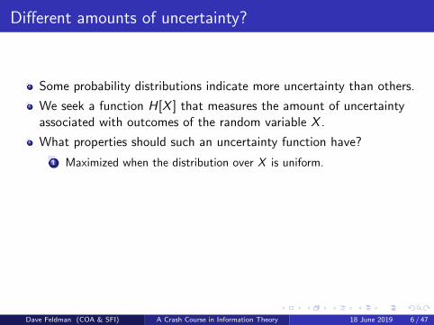
Some probability distributions indicate more uncertainty than others.
We seek a function H[X ] that measures the amount of uncertaintyassociated with outcomes of the random variable X .
What properties should such an uncertainty function have?
1 Maximized when the distribution over X is uniform.2 Continuous function of the probabilities of the different outcomes of X3 Independent of the way in which we might group probabilities.
H(p1, p2, . . . , pm) = H(p1 + p2, p3, . . . , pm) + (p1 + p2)H
(p1
p1 + p2,
p2p1 + p2
)
Dave Feldman (COA & SFI) A Crash Course in Information Theory 18 June 2019 6 / 47
Different amounts of uncertainty?
Some probability distributions indicate more uncertainty than others.
We seek a function H[X ] that measures the amount of uncertaintyassociated with outcomes of the random variable X .
What properties should such an uncertainty function have?
1 Maximized when the distribution over X is uniform.
2 Continuous function of the probabilities of the different outcomes of X3 Independent of the way in which we might group probabilities.
H(p1, p2, . . . , pm) = H(p1 + p2, p3, . . . , pm) + (p1 + p2)H
(p1
p1 + p2,
p2p1 + p2
)
Dave Feldman (COA & SFI) A Crash Course in Information Theory 18 June 2019 6 / 47

Different amounts of uncertainty?
Some probability distributions indicate more uncertainty than others.
We seek a function H[X ] that measures the amount of uncertaintyassociated with outcomes of the random variable X .
What properties should such an uncertainty function have?
1 Maximized when the distribution over X is uniform.2 Continuous function of the probabilities of the different outcomes of X
3 Independent of the way in which we might group probabilities.
H(p1, p2, . . . , pm) = H(p1 + p2, p3, . . . , pm) + (p1 + p2)H
(p1
p1 + p2,
p2p1 + p2
)
Dave Feldman (COA & SFI) A Crash Course in Information Theory 18 June 2019 6 / 47

Different amounts of uncertainty?
Some probability distributions indicate more uncertainty than others.
We seek a function H[X ] that measures the amount of uncertaintyassociated with outcomes of the random variable X .
What properties should such an uncertainty function have?
1 Maximized when the distribution over X is uniform.2 Continuous function of the probabilities of the different outcomes of X3 Independent of the way in which we might group probabilities.
H(p1, p2, . . . , pm) = H(p1 + p2, p3, . . . , pm) + (p1 + p2)H
(p1
p1 + p2,
p2p1 + p2
)
Dave Feldman (COA & SFI) A Crash Course in Information Theory 18 June 2019 6 / 47

Entropy of a Single Variable
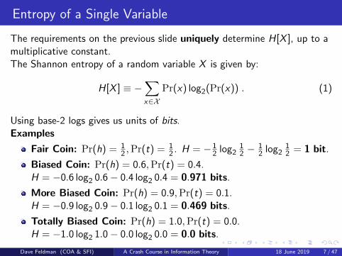
The requirements on the previous slide uniquely determine H[X ], up to amultiplicative constant.The Shannon entropy of a random variable X is given by:
H[X ] ≡ −∑x∈X
Pr(x) log2(Pr(x)) . (1)
Using base-2 logs gives us units of bits.
Examples
Fair Coin: Pr(h) = 12 ,Pr(t) = 1
2 . H = −12 log2
12 −
12 log2
12 = 1 bit.
Biased Coin: Pr(h) = 0.6,Pr(t) = 0.4.H = −0.6 log2 0.6− 0.4 log2 0.4 = 0.971 bits.
More Biased Coin: Pr(h) = 0.9,Pr(t) = 0.1.H = −0.9 log2 0.9− 0.1 log2 0.1 = 0.469 bits.
Totally Biased Coin: Pr(h) = 1.0,Pr(t) = 0.0.H = −1.0 log2 1.0− 0.0 log2 0.0 = 0.0 bits.
Dave Feldman (COA & SFI) A Crash Course in Information Theory 18 June 2019 7 / 47
Entropy of a Single Variable
The requirements on the previous slide uniquely determine H[X ], up to amultiplicative constant.The Shannon entropy of a random variable X is given by:
H[X ] ≡ −∑x∈X
Pr(x) log2(Pr(x)) . (1)
Using base-2 logs gives us units of bits.Examples
Fair Coin: Pr(h) = 12 ,Pr(t) = 1
2 . H = −12 log2
12 −
12 log2
12 = 1 bit.
Biased Coin: Pr(h) = 0.6,Pr(t) = 0.4.H = −0.6 log2 0.6− 0.4 log2 0.4 = 0.971 bits.
More Biased Coin: Pr(h) = 0.9,Pr(t) = 0.1.H = −0.9 log2 0.9− 0.1 log2 0.1 = 0.469 bits.
Totally Biased Coin: Pr(h) = 1.0,Pr(t) = 0.0.H = −1.0 log2 1.0− 0.0 log2 0.0 = 0.0 bits.
Dave Feldman (COA & SFI) A Crash Course in Information Theory 18 June 2019 7 / 47

Binary Entropy
Entropy of a binary variable as a function of its bias.Figure Source: original work by Brona, published at https://commons.wikimedia.org/wiki/File:Binary_entropy_plot.svg.
Dave Feldman (COA & SFI) A Crash Course in Information Theory 18 June 2019 8 / 47

Average Surprise
− log2 Pr(x) may be viewed as the surprise associated with theoutcome x .
Thus, H[X ] is the average, or expected value, of the surprise:
H[X ] =∑x
[− log2 Pr(x) ]Pr(x) .
The more surprised you are about a measurement, the moreinformative it is.
The greater H[X ], the more informative, on average, a measurementof X is.
Dave Feldman (COA & SFI) A Crash Course in Information Theory 18 June 2019 9 / 47
Guessing Games 1
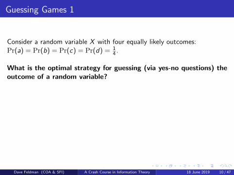
Consider a random variable X with four equally likely outcomes:Pr(a) = Pr(b) = Pr(c) = Pr(d) = 1
4 .
What is the optimal strategy for guessing (via yes-no questions) theoutcome of a random variable?
1 “is X equal to a or b?”
2 If yes, “is X = a?” If no, “is X = c?”
Using this strategy, it will always take 2 guesses.H[X ] = 2. Coincidence???
Dave Feldman (COA & SFI) A Crash Course in Information Theory 18 June 2019 10 / 47

Guessing Games 1
Consider a random variable X with four equally likely outcomes:Pr(a) = Pr(b) = Pr(c) = Pr(d) = 1
4 .
What is the optimal strategy for guessing (via yes-no questions) theoutcome of a random variable?
1 “is X equal to a or b?”
2 If yes, “is X = a?” If no, “is X = c?”
Using this strategy, it will always take 2 guesses.H[X ] = 2. Coincidence???
Dave Feldman (COA & SFI) A Crash Course in Information Theory 18 June 2019 10 / 47
Guessing Games 2
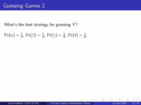
What’s the best strategy for guessing Y ?
Pr(α) = 12 , Pr(β) = 1
4 , Pr(γ) = 18 , Pr(δ) = 1
8 .
1 Is it α? If yes, then done, if no:
2 Is it β? If yes, then done, if no:
3 Is it γ? Either answer, done.
Ave # of guesses = 12(1) + 1
4(2) + 14(3) = 1.75.
Not coincidentally, H[Y ] = 1.75!!
Dave Feldman (COA & SFI) A Crash Course in Information Theory 18 June 2019 11 / 47

Guessing Games 2
What’s the best strategy for guessing Y ?
Pr(α) = 12 , Pr(β) = 1
4 , Pr(γ) = 18 , Pr(δ) = 1
8 .
1 Is it α? If yes, then done, if no:
2 Is it β? If yes, then done, if no:
3 Is it γ? Either answer, done.
Ave # of guesses = 12(1) + 1
4(2) + 14(3) = 1.75.
Not coincidentally, H[Y ] = 1.75!!
Dave Feldman (COA & SFI) A Crash Course in Information Theory 18 June 2019 11 / 47

Entropy Measures Average Number of Guesses
Strategy: try to divide the probability in half with each guess.
General result: Average number of yes-no questions needed toguess the outcome of X is between H[X ] and H[X ] + 1.
This is consistent with the interpretation of H as uncertainty.
If the probability is concentrated more on some outcomes than others,we can exploit this regularity to make more efficient guesses.
Dave Feldman (COA & SFI) A Crash Course in Information Theory 18 June 2019 12 / 47

Coding
A code is a mapping from a set of symbols to another set of symbols.
Here, we are interested in a code for the possible outcomes of arandom variable that is as short as possible while still being decodable.
Strategy: use short code words for more common occurrences of X .
This is identical to the strategy for guessing outcomes.
Example: Optimal binary code for Y :
α −→ 1 , β −→ 01
γ −→ 001 , δ −→ 000
Note: This code is unambiguously decodable:
0110010000000101 = βαγδδββ
This type of code is called an instantaneous code.
Dave Feldman (COA & SFI) A Crash Course in Information Theory 18 June 2019 13 / 47

Coding, continued
Shannon’s noiseless source coding theorem:
Average number of bits in optimal binary code for X is betweenH[X ] and H[X ] + 1.
Also known as Shannon’s first theorem.
Thus, H[X ] is the average memory, in bits, needed to store outcomes ofthe random variable X .
Dave Feldman (COA & SFI) A Crash Course in Information Theory 18 June 2019 14 / 47

Summary of interpretations of entropy
H[X ] is the measure of uncertainty associated with the distribution ofX .
Requiring H to be a continuous function of the distribution,maximized by the uniform distribution, and independent of themanner in which subsets of events are grouped, uniquely determinesH.
H[X ] is the expectation value of the surprise, − log2 Pr(x).
H[X ] ≤ Average number of yes-no questions needed to guess theoutcome of X ≤ H[X ] + 1.
H[X ] ≤ Average number of bits in optimal binary code for X≤ H[X ] + 1.
H[X ] = limN →∞ 1N× average length of optimal binary code of N
copies of X .
Dave Feldman (COA & SFI) A Crash Course in Information Theory 18 June 2019 15 / 47

Joint and Conditional Entropies
Joint Entropy
H[X ,Y ] ≡ −∑
x∈X∑
y∈Y Pr(x , y) log2(Pr(x , y))
H[X ,Y ] is the uncertainty associated with the outcomes of X and Y .
Conditional Entropy
H[X |Y ] ≡ −∑
x∈X∑
y∈Y Pr(x , y) log2 Pr(x |y) .
H[X |Y ] is the average uncertainty of X given that Y is known.
Relationships
H[X ,Y ] = H[X ] + H[Y |X ]
H[Y |X ] = H[X ,Y ]− H[X ]
H[Y |X ] 6= H[X |Y ]
Dave Feldman (COA & SFI) A Crash Course in Information Theory 18 June 2019 16 / 47

Mutual Information
Definition
I [X ;Y ] = H[X ]− H[X |Y ]
I [X ;Y ] is the average reduction in uncertainty of X given knowledgeof Y .
Relationships
I [X ;Y ] = H[X ]− H[X |Y ]
I [X ;Y ] = H[Y ]− H[Y |X ]
I [X ;Y ] = H[Y ] + H[X ]− H[X ,Y ]
I [X ;Y ] = I [Y ;X ]
Dave Feldman (COA & SFI) A Crash Course in Information Theory 18 June 2019 17 / 47

Information Diagram
The information diagram shows the relationship among joint andconditional entropies and the mutual information.Figure Source: Konrad Voelkel, released to the public domain.
https://commons.wikimedia.org/wiki/File:Entropy-mutual-information-relative-entropy-relation-diagram.svg
Dave Feldman (COA & SFI) A Crash Course in Information Theory 18 June 2019 18 / 47

Example 1
Two independent, fair coins, C1 and C2.
C1 C2
h t
h 14
14
t 14
14
H[C1] = 1 and H[C2] = 1.
H[C1,C2] = 2.
H[C1|C2] = 1. Even if you know what C2 is, you’re still uncertainabout C1.
I [C1;C2] = 0. Knowing C1 does not reduce your uncertainty of C2 atall.
C1 carries no information about C2.
Dave Feldman (COA & SFI) A Crash Course in Information Theory 18 June 2019 19 / 47
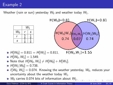
Example 2
Weather (rain or sun) yesterday W0 and weather today W1.
W1
W0 r s
r 58
18
s 18
18
H[W0] = 0.811 = H[W1] = 0.811.
H[W0,W1] = 1.549.
Note that H[W0,W1] 6= H[W0] + H[W1].
H[W1|W0] = 0.738.
I [W0;W1] = 0.074. Knowing the weather yesterday, W0, reduces youruncertainty about the weather today W1.
W0 carries 0.074 bits of information about W1.
Dave Feldman (COA & SFI) A Crash Course in Information Theory 18 June 2019 20 / 47
Estimating Entropies
By the way...
Probabilities Pr(x), etc., can be estimated empirically.
Just observe the occurrences ci of different outcomes and estimatethe frequencies:
Pr(xi ) =ci∑j cj
.
No big deal.
However, this will lead to a biased under-estimate for H[X ]. For moreaccurate ways of estimate H[X ], see, e.g.,
Schurmann and Grassberger. Chaos 6:414-427. 1996.
Kraskov, Stogbauer, and Grassberger. Phys Rev E 69.6: 066138. 2004.
Dave Feldman (COA & SFI) A Crash Course in Information Theory 18 June 2019 21 / 47

Application: Maximum Entropy
A common technique in statistical inference is the maximumentropy method.
Suppose we know a number of average properties of a randomvariable. We want to know what distribution the random variablecomes from.
This is an underspecified problem. What to do?
Choose the distribution that maximizes the entropy while still yieldingthe correct average values.
This is usually accomplished by using Lagrange multipliers to performa constrained maximization.
The justification for the maximum entropy method is that it assumesno information beyond what is already known in the form of theaverage values.
Dave Feldman (COA & SFI) A Crash Course in Information Theory 18 June 2019 22 / 47
Relative Entropy
The Relative Entropy or the Kullback-Leibler distance between twodistributions p(x) and q(x) is:
D(p||q) ≡∑x∈X
p(x) log2p(x)
q(x).
D(p||q) is how much more random X appears if one assumes it isdistributed according to q when it is actually distributed according to p.
D(p||q) is measure of “entropic distance” between p and q.
Dave Feldman (COA & SFI) A Crash Course in Information Theory 18 June 2019 23 / 47

Relative Entropy: Example
X ∈ {a, b, c, d}p : p(a) = 1/2, p(b) = 1/4, p(c) = 1/8, p(d) = 1/8q : q(a) = 1/4, q(b) = 1/4, q(c) = 1/4, q(d) = 1/4
D(p||q) ≡∑x∈X
p(x) log2p(x)
q(x),
D(p||q) ≡∑x∈X−p(x) log2 q(x)− H(p) .
The first term on the right is the expected code length if we used the codefor q for a variable that was actually distributed according to p.
Dave Feldman (COA & SFI) A Crash Course in Information Theory 18 June 2019 24 / 47
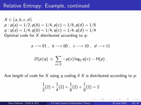
Relative Entropy: Example, continued
X ∈ {a, b, c, d}p : p(a) = 1/2, p(b) = 1/4, p(c) = 1/8, p(d) = 1/8q : q(a) = 1/4, q(b) = 1/4, q(c) = 1/4, q(d) = 1/4Optimal code for X distributed according to q:
a −→ 01 , b −→ 00 , c −→ 10 , d −→ 11
D(p||q) ≡∑x∈X−p(x) log2 q(x)− H(p) .
Ave length of code for X using q coding if X is distributed according to p:
1
2(2) +
1
4(2) +
1
8(2) +
1
8(2) = 2
Dave Feldman (COA & SFI) A Crash Course in Information Theory 18 June 2019 25 / 47

Relative Entropy: Example, continued further
X ∈ {a, b, c, d}p : p(a) = 1/2, p(b) = 1/4, p(c) = 1/8, p(d) = 1/8q : q(a) = 1/4, q(b) = 1/4, q(c) = 1/4, q(d) = 1/4
Recall that H(p) = 1.75. Then
D(p||q) ≡∑x∈X−p(x) log2 q(x)− H(p) .
D(p||q) = 2− 1.75 = 0.25 .
So using the code for q when X is distributed according to p adds 0.25 tothe average code length.
Exercise: Show that D(q||p) = 0.25.
Dave Feldman (COA & SFI) A Crash Course in Information Theory 18 June 2019 26 / 47
Relative Entropy Summary
D(p||q) is not a proper distance. It is not symmetric and does notobey the triangle inequality.
Arises in many different learning/adapting and statistics contexts.
Measures the “coding mismatch” or “entropic distance” between pand q.
Dave Feldman (COA & SFI) A Crash Course in Information Theory 18 June 2019 27 / 47

Summary and Reflections
Information theory provides a natural language for working withprobabilities.
Information theory is not a theory of semantics or meaning.
Information theory is used throughout complex systems.
Information theory complements computation theory.
Computation theory: worst case scenarioInformation theory: average scenario
Often shows common mathematical structures across differentdomains and contexts.
Dave Feldman (COA & SFI) A Crash Course in Information Theory 18 June 2019 28 / 47

Information Theory: Part II Applications to StochasticProcesses
We now consider applying information theory to a long sequence ofmeasurements.
· · · 00110010010101101001100111010110 · · ·
In so doing, we will be led to two important quantities1 Entropy Rate: The irreducible randomness of the system.2 Excess Entropy: A measure of the complexity of the sequence.
Context: Consider a long sequence of discrete random variables.These could be:
1 A long time series of measurements2 A symbolic dynamical system3 A one-dimensional statistical mechanical system
Dave Feldman (COA & SFI) A Crash Course in Information Theory 18 June 2019 29 / 47

Stochastic Process Notation
Random variables Si , Si = s ∈ A.
Infinite sequence of random variables:↔S = . . . S−1 S0 S1 S2 . . .
Block of L consecutive variables: SL = S1, . . . ,SL.
Pr(si , si+1, . . . , si+L−1) = Pr(sL)
Assume translation invariance or stationarity:
Pr( si, si+1, · · · , si+L−1 ) = Pr( s1, s2, · · · , sL ) .
Left half (“past”):←s ≡ · · ·S−3 S−2 S−1
Right half (“future”):→s ≡ S0 S1 S2 · · ·
· · · 11010100101101010101001001010010 · · ·
Dave Feldman (COA & SFI) A Crash Course in Information Theory 18 June 2019 30 / 47

Entropy Growth
Entropy of L-block:
H(L) ≡ −∑
sL∈AL
Pr(sL) log2 Pr(sL) .
H(L) = average uncertainty about the outcome of L consecutivevariables.
0
0.5
1
1.5
2
2.5
3
3.5
4
0 1 2 3 4 5 6 7 8
H(L
)
LH(L) increases monotonically and asymptotes to a line
We can learn a lot from the shape of H(L).
Dave Feldman (COA & SFI) A Crash Course in Information Theory 18 June 2019 31 / 47

Entropy Rate
Let’s first look at the slope of the line:
0 L
H(L)
µ+ h L
E
E
H(L)
Slope of H(L): hµ(L) ≡ H(L)− H(L−1)
Slope of the line to which H(L) asymptotes is known as the entropyrate:
hµ = limL→∞
hµ(L).
Dave Feldman (COA & SFI) A Crash Course in Information Theory 18 June 2019 32 / 47

Entropy Rate, continued
Slope of the line to which H(L) asymptotes is known as the entropyrate:
hµ = limL→∞
hµ(L).
hµ(L) = H[SL|S1S1 . . . SL−1]
I.e., hµ(L) is the average uncertainty of the next symbol, given thatthe previous L symbols have been observed.
Dave Feldman (COA & SFI) A Crash Course in Information Theory 18 June 2019 33 / 47

Interpretations of Entropy Rate
Uncertainty per symbol.
Irreducible randomness: the randomness that persists even afteraccounting for correlations over arbitrarily large blocks of variables.
The randomness that cannot be “explained away”.
Entropy rate is also known as the Entropy Density or the MetricEntropy.
hµ = Lyapunov exponent for many classes of 1D maps.
The entropy rate may also be written: hµ = limL→∞H(L)L .
hµ is equivalent to thermodynamic entropy.
These limits exist for all stationary processes.
Dave Feldman (COA & SFI) A Crash Course in Information Theory 18 June 2019 34 / 47

How does hµ(L) approach hµ?
For finite L , hµ(L) ≥ hµ. Thus, the system appears more randomthan it is.
1 L
h (L)µ
hµ
E
H(1)
We can learn about the complexity of the system by looking at howthe entropy density converges to hµ.
Dave Feldman (COA & SFI) A Crash Course in Information Theory 18 June 2019 35 / 47
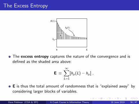
The Excess Entropy
1 L
h (L)µ
hµ
E
H(1)
The excess entropy captures the nature of the convergence and isdefined as the shaded area above:
E ≡∞∑L=1
[hµ(L)− hµ] .
E is thus the total amount of randomness that is “explained away” byconsidering larger blocks of variables.
Dave Feldman (COA & SFI) A Crash Course in Information Theory 18 June 2019 36 / 47
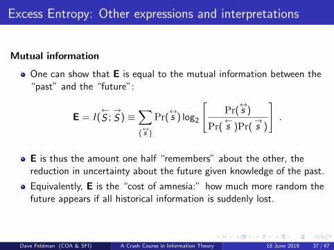
Excess Entropy: Other expressions and interpretations
Mutual information
One can show that E is equal to the mutual information between the“past” and the “future”:
E = I (←S ;→S ) ≡
∑{↔s }
Pr(↔s ) log2
[Pr(↔s )
Pr(←s )Pr(
→s )
].
E is thus the amount one half “remembers” about the other, thereduction in uncertainty about the future given knowledge of the past.
Equivalently, E is the “cost of amnesia:” how much more random thefuture appears if all historical information is suddenly lost.
Dave Feldman (COA & SFI) A Crash Course in Information Theory 18 June 2019 37 / 47

Excess Entropy: Other expressions and interpretations
Geometric View
E is the y -intercept of the straight line to which H(L) asymptotes.
E = limL→∞ [H(L) − hµL] .
0 L
H(L)
µ+ h L
E
E
H(L)
Dave Feldman (COA & SFI) A Crash Course in Information Theory 18 June 2019 38 / 47

Excess Entropy Summary
Is a structural property of the system — measures a featurecomplementary to entropy.
Measures memory or spatial structure.
Lower bound for statistical complexity, minimum amount ofinformation needed for minimal stochastic model of system
Dave Feldman (COA & SFI) A Crash Course in Information Theory 18 June 2019 39 / 47

Example I: Fair Coin
0
2
4
6
8
10
12
14
16
0 2 4 6 8 10 12 14
H(L
)
L
H(L): Fair Coin
H(L): Biased Coin, p=.7
For fair coin, hµ = 1.
For the biased coin, hµ ≈ 0.8831.
For both coins, E = 0.
Note that two systems with different entropy rates have the sameexcess entropy.
Dave Feldman (COA & SFI) A Crash Course in Information Theory 18 June 2019 40 / 47

Example II: Periodic Sequence
0
0.5
1
1.5
2
2.5
3
3.5
4
4.5
0 2 4 6 8 10 12 14 16 18H
(L)
L
H(L)
E + hµL
0
0.2
0.4
0.6
0.8
1
1.2
1.4
0 2 4 6 8 10 12 14 16 18
hµ
(L)
L
hµ(L)
Sequence: . . . 1010111011101110 . . .
Dave Feldman (COA & SFI) A Crash Course in Information Theory 18 June 2019 41 / 47
Example II, continued
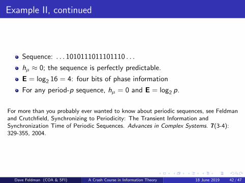
Sequence: . . . 1010111011101110 . . .
hµ ≈ 0; the sequence is perfectly predictable.
E = log2 16 = 4: four bits of phase information
For any period-p sequence, hµ = 0 and E = log2 p.
For more than you probably ever wanted to know about periodic sequences, see Feldmanand Crutchfield, Synchronizing to Periodicity: The Transient Information andSynchronization Time of Periodic Sequences. Advances in Complex Systems. 7(3-4):329-355, 2004.
Dave Feldman (COA & SFI) A Crash Course in Information Theory 18 June 2019 42 / 47

Example III: Random, Random, XOR
0
2
4
6
8
10
12
14
0 2 4 6 8 10 12 14 16 18H
(L)
L
H(L)
E + hµL
0
0.2
0.4
0.6
0.8
1
1.2
0 2 4 6 8 10 12 14 16 18
hµ(L
)
L
hµ(L)
Sequence: two random symbols, followed by the XOR of thosesymbols.
Dave Feldman (COA & SFI) A Crash Course in Information Theory 18 June 2019 43 / 47

Example III, continued
Sequence: two random symbols, followed by the XOR of thosesymbols.
hµ = 23 ; two-thirds of the symbols are unpredictable.
E = log2 4 = 2: two bits of phase information.
For many more examples, see Crutchfield and Feldman, Chaos, 15:25-54, 2003.
Dave Feldman (COA & SFI) A Crash Course in Information Theory 18 June 2019 44 / 47

Excess Entropy: Notes on Terminology
All of the following terms refer to essentially the same quantity.
Excess Entropy: Crutchfield, Packard, Feldman
Stored Information: Shaw
Effective Measure Complexity: Grassberger, Lindgren, Nordahl
Reduced (Renyi) Information: Szepfalusy, Gyorgyi, Csordas
Complexity: Li, Arnold
Predictive Information: Nemenman, Bialek, Tishby
Dave Feldman (COA & SFI) A Crash Course in Information Theory 18 June 2019 45 / 47
Excess Entropy: Selected References and Applications
Crutchfield and Packard, Intl. J. Theo. Phys, 21:433-466. (1982); PhysicaD, 7:201-223, 1983. [Dynamical systems]
Shaw, “The Dripping Faucet ..., ” Aerial Press, 1984. [A dripping faucet]
Grassberger, Intl. J. Theo. Phys, 25:907-938, 1986. [Cellular automata(CAs), dynamical systems]
Szepfalusy and Gyorgyi, Phys. Rev. A, 33:2852-2855, 1986. [Dynamicalsystems]
Lindgren and Nordahl, Complex Systems, 2:409-440. (1988). [CAs,dynamical systems]
Csordas and Szepfalusy, Phys. Rev. A, 39:4767-4777. 1989. [DynamicalSystems]
Li, Complex Systems, 5:381-399, 1991.
Freund, Ebeling, and Rateitschak, Phys. Rev. E, 54:5561-5566, 1996.
Feldman and Crutchfield, SFI:98-04-026, 1998. Crutchfield and Feldman,Phys. Rev. E 55:R1239-42. 1997. [One-dimensional Ising models]
Dave Feldman (COA & SFI) A Crash Course in Information Theory 18 June 2019 46 / 47

Excess Entropy: Selected References and Applications,continued
Feldman and Crutchfield. Physical Review E, 67:051104. 2003.[Two-dimensional Ising models]
Feixas, et al, Eurographics, Computer Graphics Forum, 18(3):95-106, 1999.[Image processing]
Ebeling. Physica D, 1090:42-52. 1997. [Dynamical systems, written texts,music]
Bialek, et al, Neur. Comp., 13:2409-2463. 2001. [Long-range 1D Isingmodels, machine learning]
Dave Feldman (COA & SFI) A Crash Course in Information Theory 18 June 2019 47 / 47