7. Lossy image compression

• Block Truncation Coding (BTC)• Transform Coding (DCT JPEG)• Transform Coding (DCT, JPEG)• Wavelet Coding (JPEG2000)

Transformation Quantization EncodingData Bitstream

Model

Slides are compiled from Alexander Kolesnikov’s image compression lecture notes

Block Truncation Coding

• Divide the image into 4×4 blocks;• Quantize the block into two representative values a and b;Quantize the block into two representative values a and b;• Encode (1) the representative values a and b

and (2) the significance map in the block.

Original Bit-plane Reconstructed

2 11 11 9

2 9 12 15

0 1 1 1

0 1 1 1

2 12 12 12

2 12 12 12

3 3 4 14

2 3 12 15

0 0 0 1

0 0 1 1

2 2 2 12

2 2 12 12

x = 7.94 q = 9 a = 2.3a=[2.3] = 2 = 4.91

q

b = 12.3σa [2.3] 2b=[12.3]=12

How to construct quantizer?

• The first two moments preserving quantization:

∑=

>=<m

iim xx

1

1 ∑=

>=<m

iim xx

1

212

222 ><−>=< xxσ

• Threshold for quantization: T=<x>; n +n =m• Threshold for quantization: T=<x>; na+nb=mbnanxm ba +>=<

222 bnanxm +>=<

bnxa ⋅−>=< σ anxb ⋅+= σ

bnanxm ba +>=<

anxa >=< σ

bnxb ⋅+= σ

Example of BTC

Original Bit-plane Reconstructed

2 11 11 9

2 9 12 15

0 1 1 1

0 1 1 1

2 12 12 12

2 12 12 12

3 3 4 14

2 3 12 15

0 0 0 1

0 0 1 1

2 2 2 12

2 2 12 12

T 9x = 7.94

= 4.91

q = 9 a = 2.3

b = 12.3σT= 9na=7nb=9

5043722D

a=[2.3] = 2b=[12.3]=12

5043722 =+=+= baD σσ

2 3 4 5 6 7 8 9 10 11 12 13 14 15a bT

Representative levels compression

• Main idea of BTC:

Image → ”smooth part” + ”detailed part” (a and b) (bit-planes)

• We can treat set of a’s and b’s as an image:1. Predictive encoding of a and b2. Lossy compression: DCT (JPEG)

Bitrate and Block size

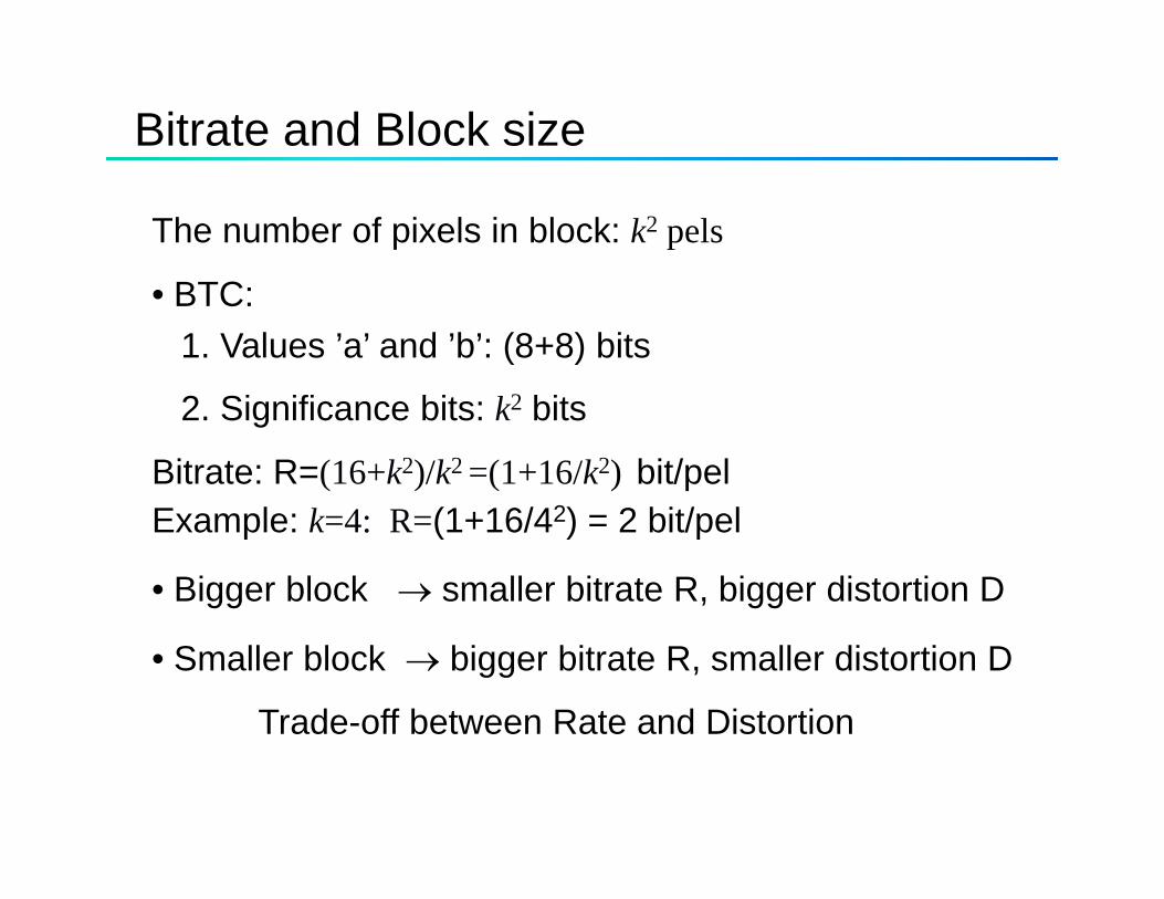
The number of pixels in block: k2 pels

• BTC: 1. Values ’a’ and ’b’: (8+8) bits

2. Significance bits: k2 bits

Bitrate: R=(16+k2)/k2 =(1+16/k2) bit/pel2Example: k=4: R=(1+16/42) = 2 bit/pel

• Bigger block → smaller bitrate R, bigger distortion D

• Smaller block → bigger bitrate R, smaller distortion D

Trade-off between Rate and DistortionTrade off between Rate and Distortion

8. JPEG

• JPEG = Joint Photographic Experts Group

• Lossy coding of continuous tone still images (color andgrayscale)

• Based on Discrete Cosine Transform (DCT):

0) Image is divided into block N×N

) h bl k f d h 2 C1) The blocks are transformed with 2-D DCT

2) DCT coefficients are quantized

3) Th ti d ffi i t d d3) The quantized coefficients are encoded

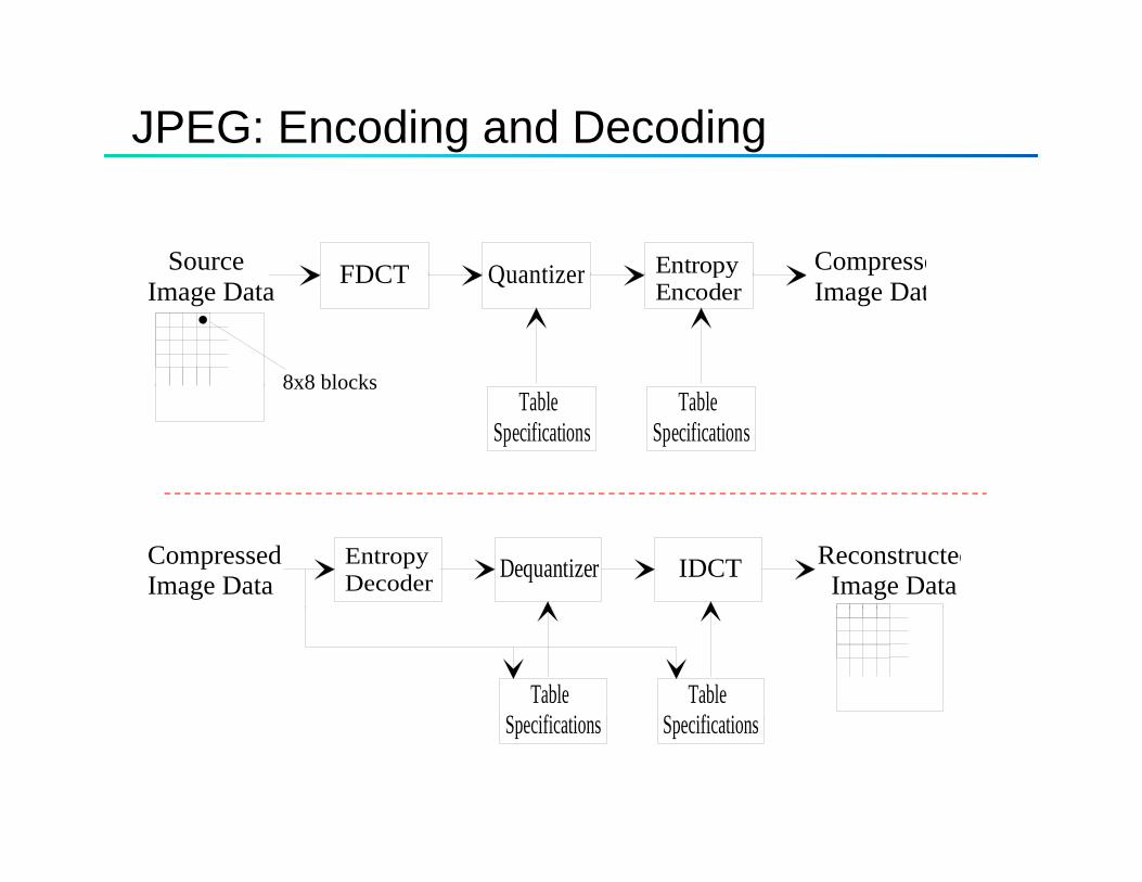
JPEG: Encoding and Decoding

Source FDCT Quantizer Entropy CompresseImage Data

8x8 blocks

FDCT Quantizer pyEncoder

pImage Dat

8x8 blocks TableSpecifications

TableSpecifications

IDCTDequantizerEntropyDecoder

Reconstructed Image Data

CompressedImage Data

TableS ifi ti

TableS ifi tiSpecifications Specifications

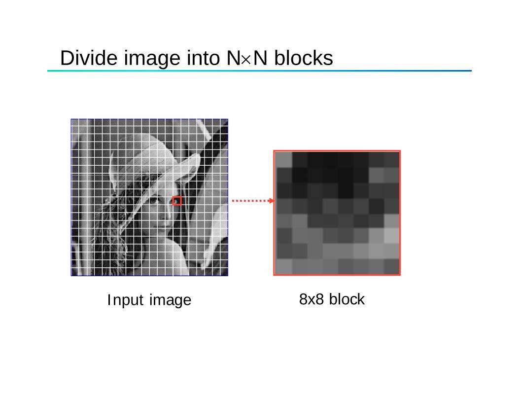
Divide image into N×N blocks

8x8 blockInput image

2-D DCT basis functions: N=8

Low Higho

LowHigh

Low

High High

8x8 block

High High

HighLow

2-D Transform Coding

+y00y01 y10

y12y23y01 y10

y12

...

1-D DCT basis functions: N=8

1.0u=0

1.0u=1

1.0u=2

1.0u=3

0.5

0

-0.5

0.5

0

-0.5

0.5

0

-0.5

0.5

0

-0.5

-1.0 -1.0 -1.0 -1.0

1.0

0 5

u=41.0

0 5

u=51.0

0 5

u=61.0

0 5

u=7

0.5

0

-0.5

-1.0

0.5

0

-0.5

-1.0

0.5

0

-0.5

-1.0

0.5

0

-0.5

-1.0

( ) ( ) ( )∑−

⎥⎦⎤

⎢⎣⎡ +

⋅=1

212cos

N

j NkjkCkx πα ( )

⎪

⎪⎨

⎧ ==

121f2

0for 1

Nk

kNkα∑=

⎥⎦⎢⎣0 2kj N ⎪

⎩−= 1,...,2,1for 2 NkN

2-D DCT basis functions: N=M = 8where

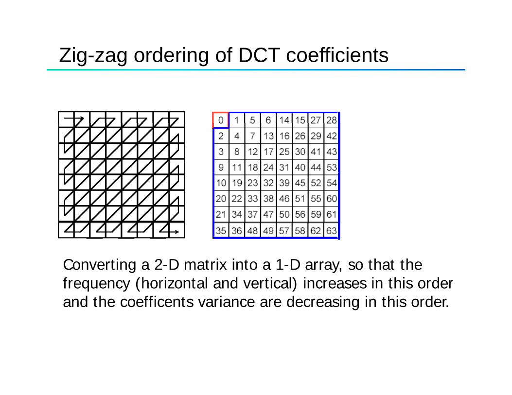
Zig-zag ordering of DCT coefficients

Converting a 2-D matrix into a 1-D array, so that the g y,frequency (horizontal and vertical) increases in this orderand the coefficents variance are decreasing in this order.

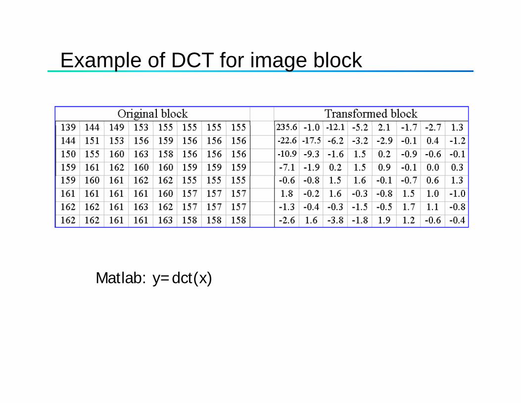
Example of DCT for image block

Matlab: y=dct(x)Matlab: y=dct(x)

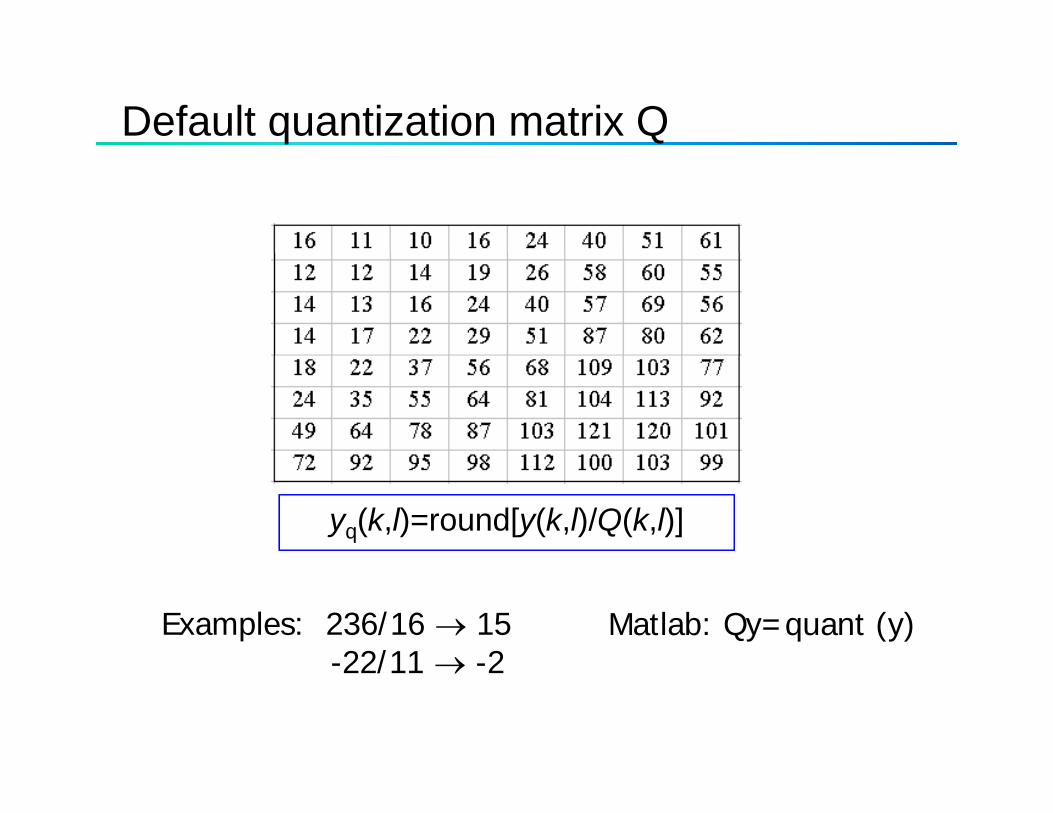
Default quantization matrix Q

yq(k,l)=round[y(k,l)/Q(k,l)]

Examples: 236/16 → 15-22/11 → -2

Matlab: Qy=quant (y)-22/11 → -2

Quantization of DCT coefficients: Example

Ordered DCT coefficients: 15,0,-2,-1,-1,-1,0,0,-1,-1, 54{’0’}.

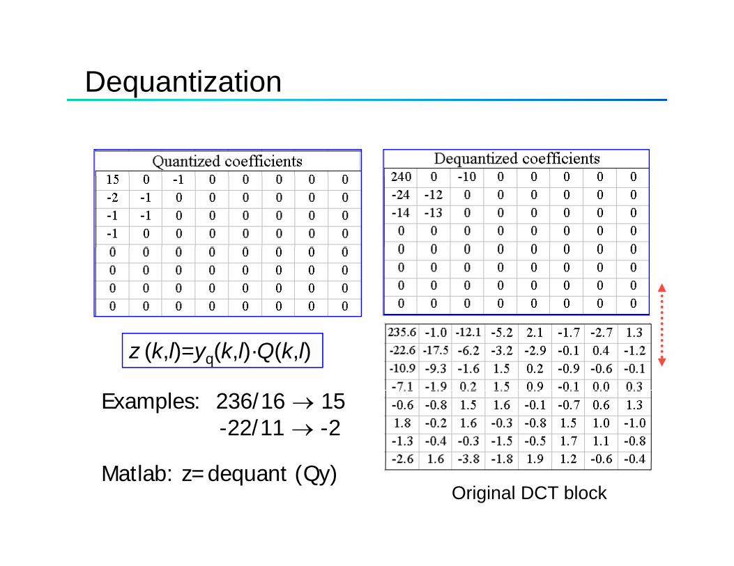
Dequantization

z (k,l)=yq(k,l)·Q(k,l)

Examples: 236/16 → 15-22/11 → -2

Original DCT blockMatlab: z=dequant (Qy)

Inverse DCT

See: x=idct(y)See: x=idct(y)

Original block

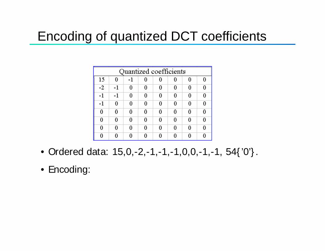
Encoding of quantized DCT coefficients

• Ordered data: 15,0,-2,-1,-1,-1,0,0,-1,-1, 54{’0’}.

• Encoding: g

Encoding of quantized DCT coefficients

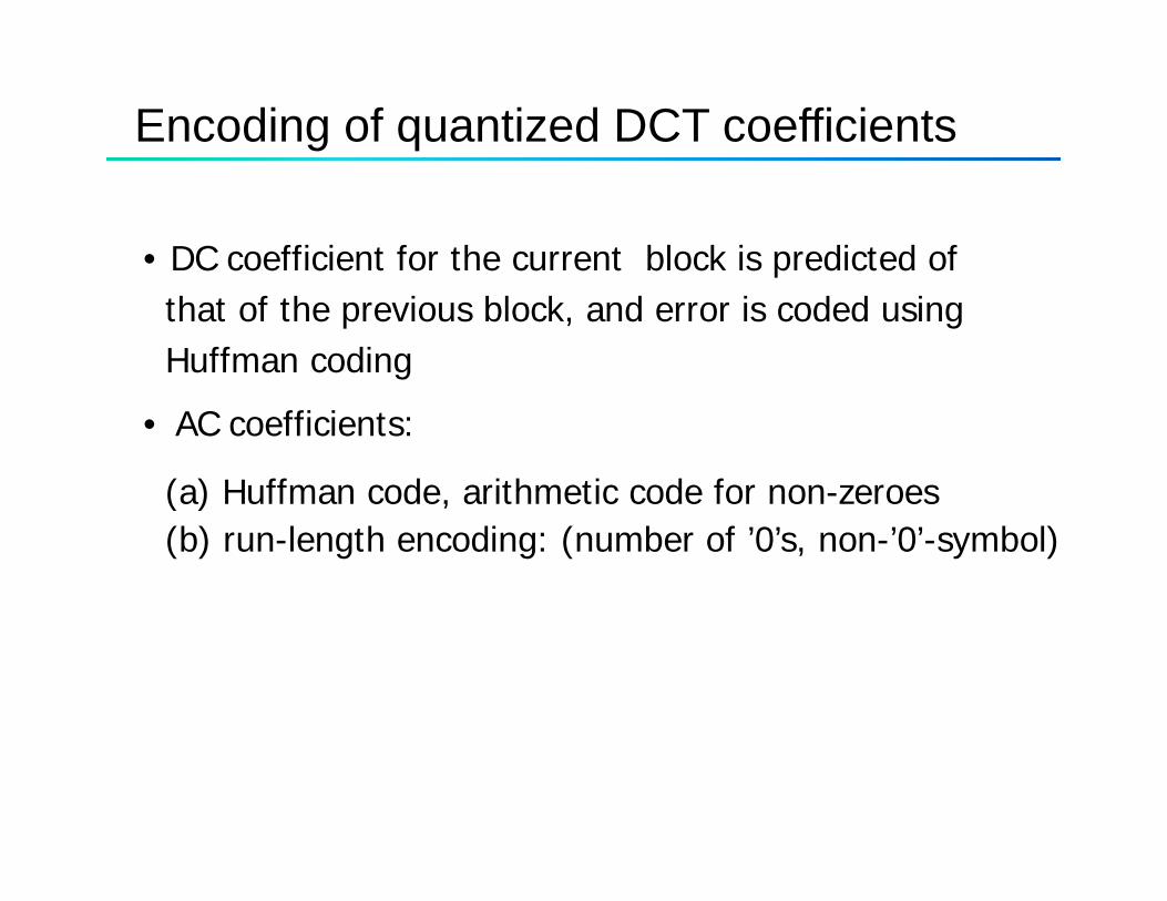
• DC coefficient for the current block is predicted of that of the previous block, and error is coded usingHuffman coding

• AC coefficients:

(a) Huffman code, arithmetic code for non-zeroes( ) ,(b) run-length encoding: (number of ’0’s, non-’0’-symbol)

Performance of JPEG algorithm

8 bpp 0.6 bpp

0.37 bpp 0.22 bpp

Compression of color images

Performance of JPEG algorithm

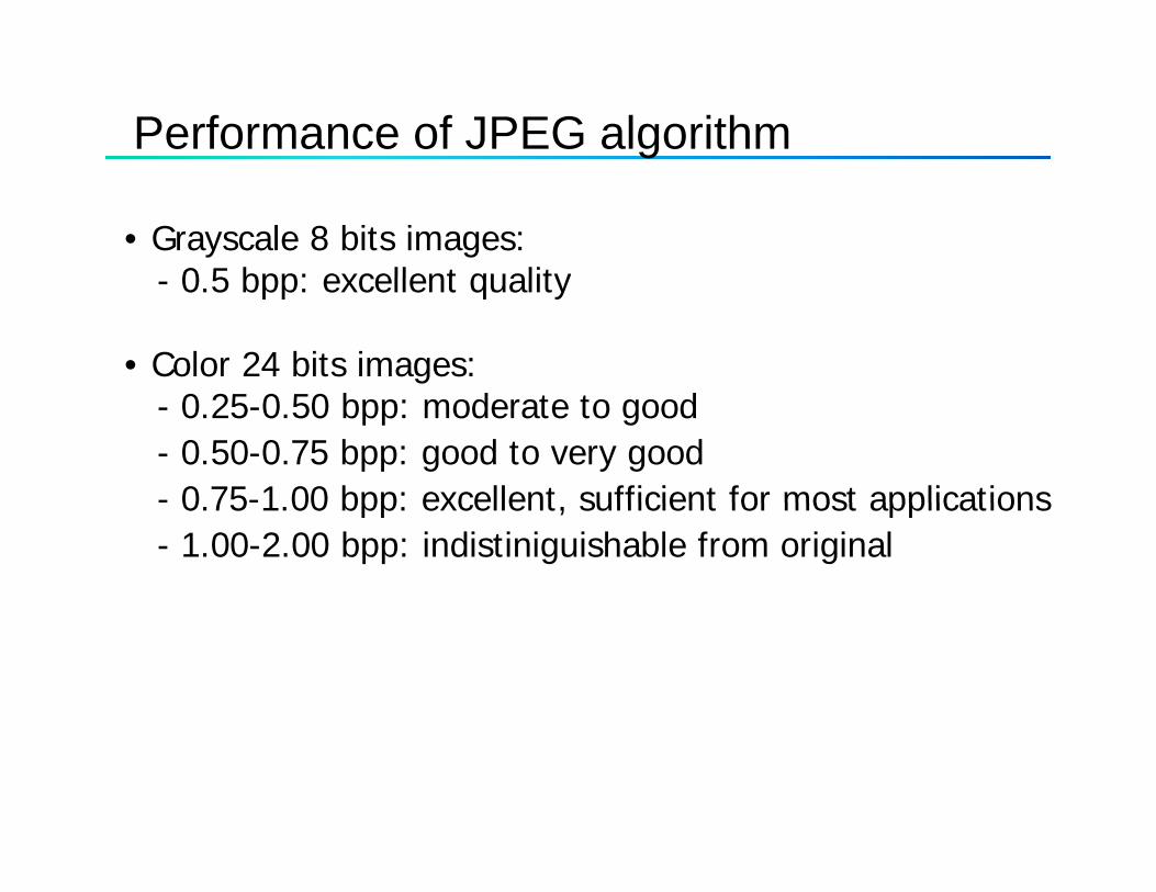
• Grayscale 8 bits images: 0 5 bpp: excellent quality- 0.5 bpp: excellent quality

• Color 24 bits images: - 0.25-0.50 bpp: moderate to good - 0.50-0.75 bpp: good to very good- 0 75-1 00 bpp: excellent sufficient for most applications0.75 1.00 bpp: excellent, sufficient for most applications - 1.00-2.00 bpp: indistiniguishable from original

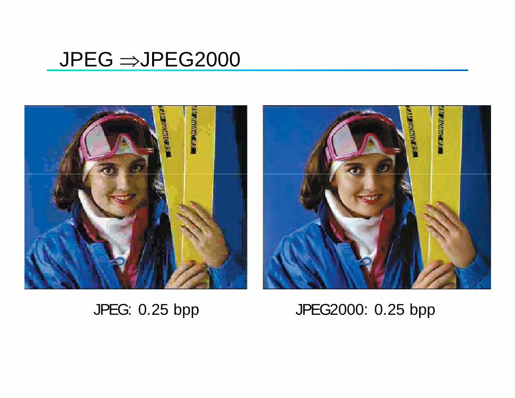
JPEG ⇒JPEG2000

For illuminanceFor illuminance

JPEG: 0.25 bpp JPEG2000: 0.25 bpp

9. JPEG 2000

• JPEG 2000 is a new still image compression standard• ”One for all” image codec:• One-for-all image codec:

* Different image types: binary, grey-scale, color, multi-componentmulti-component

* Different applications: natural images, scientific, medical remote sensing text rendered graphicsmedical remote sensing text, rendered graphics

* Different imaging models: client/server, consumer electronics, image library archival, limited bufferelectronics, image library archival, limited buffer and resources.

History

• Call for Contributions in 1996Call for Contributions in 1996• The 1st Committee Draft (CD) Dec. 1999• Final Committee Draft (FCD) in March 2000( )• Accepted as Draft International Standard in Aug. 2000• Published as ISO Standard in Jan. 2002

Key components

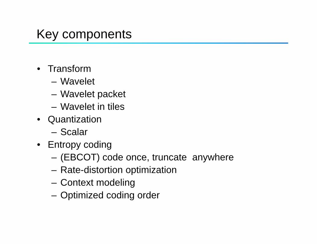
• Transform– Wavelet – Wavelet packet

Wavelet in tiles– Wavelet in tiles• Quantization

– Scalar • Entropy coding

– (EBCOT) code once, truncate anywhere Rate distortion optimization– Rate-distortion optimization

– Context modeling– Optimized coding orderp g

Key components

VisualVisualWeightingMaskingMasking

Region of interest (ROI)Lossless color transformError resilience

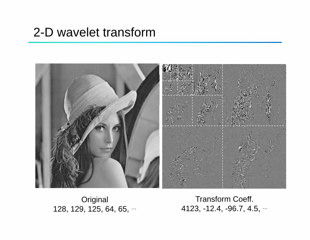
2-D wavelet transform

Original128, 129, 125, 64, 65, …

Transform Coeff.4123, -12.4, -96.7, 4.5, …

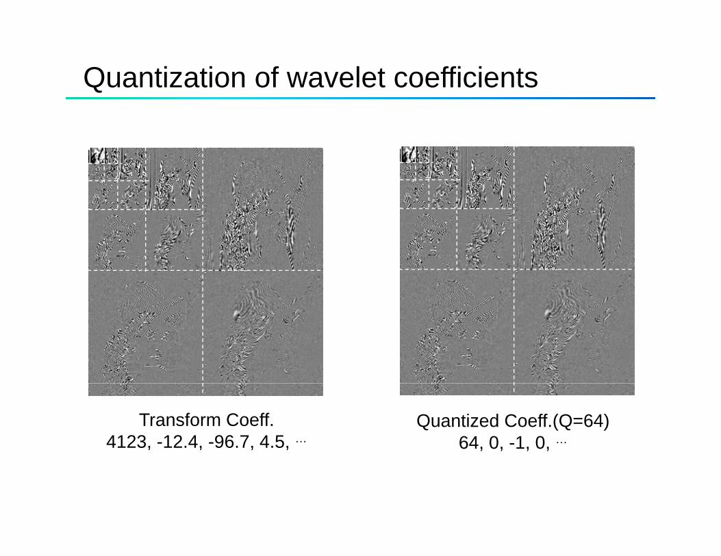
Quantization of wavelet coefficients

Transform Coeff.4123, -12.4, -96.7, 4.5, …

Quantized Coeff.(Q=64)64, 0, -1, 0, …

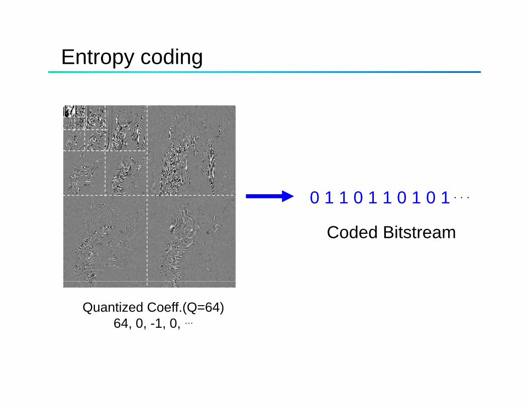
Entropy coding

0 1 1 0 1 1 0 1 0 1 . . .

Coded BitstreamCoded Bitstream

Quantized Coeff.(Q=64)64, 0, -1, 0, …

Progressive encoding

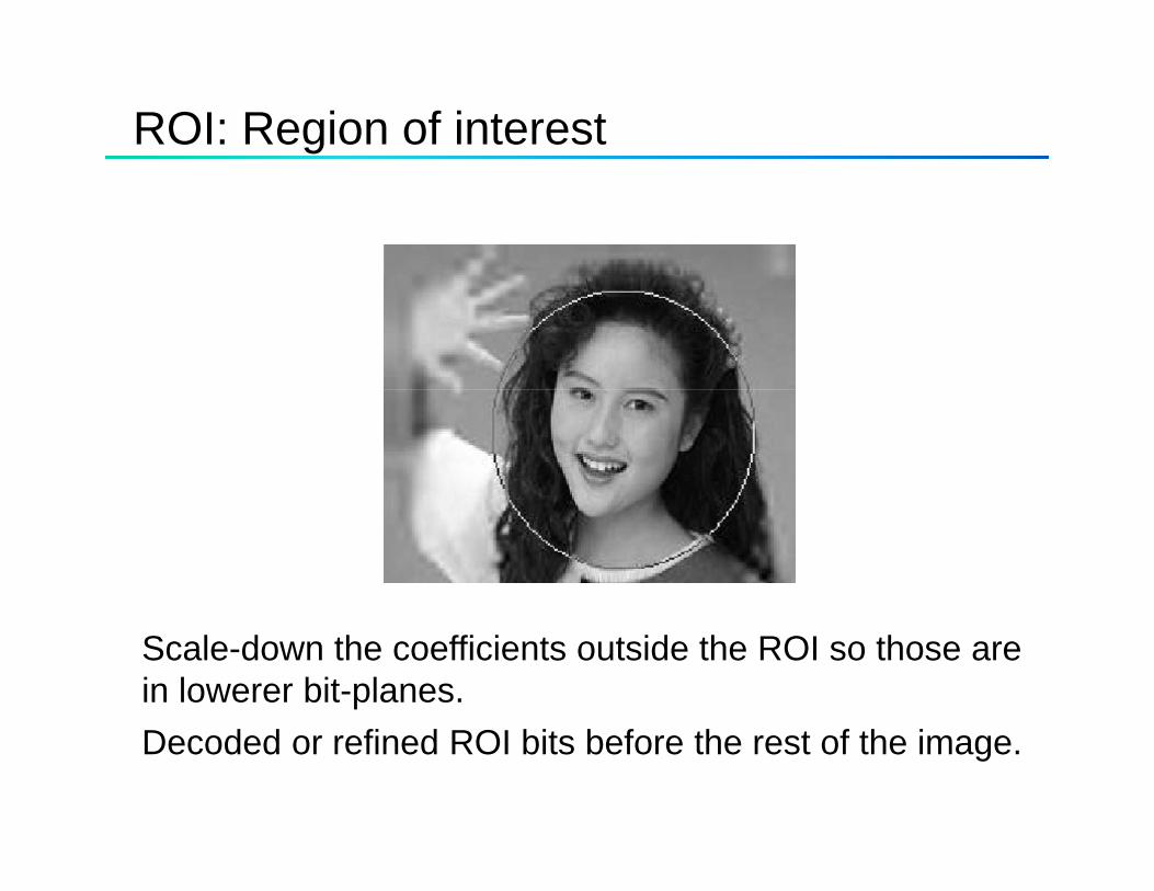
ROI: Region of interest

Scale-down the coefficients outside the ROI so those are in lowerer bit-planes.Decoded or refined ROI bits before the rest of the image.

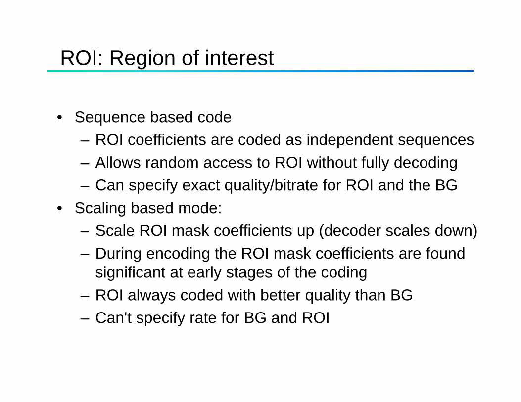
ROI: Region of interest

• Sequence based codeq– ROI coefficients are coded as independent sequences– Allows random access to ROI without fully decoding– Can specify exact quality/bitrate for ROI and the BG

• Scaling based mode:S l ROI k ffi i t (d d l d )– Scale ROI mask coefficients up (decoder scales down)

– During encoding the ROI mask coefficients are found significant at early stages of the codingsignificant at early stages of the coding

– ROI always coded with better quality than BG– Can't specify rate for BG and ROI

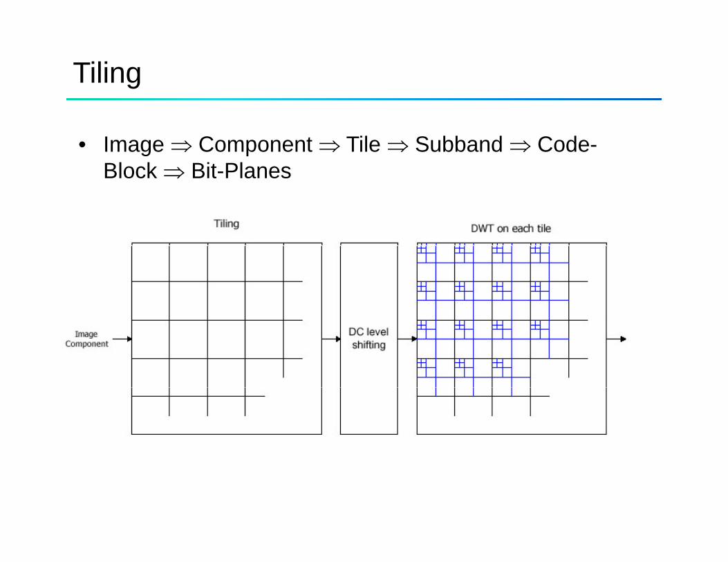
Tiling

• Image ⇒ Component ⇒ Tile ⇒ Subband ⇒ Code-Block ⇒ Bit-PlanesBlock ⇒ Bit Planes

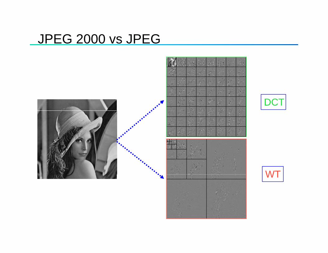
JPEG 2000 vs JPEG

DCT

WTWT

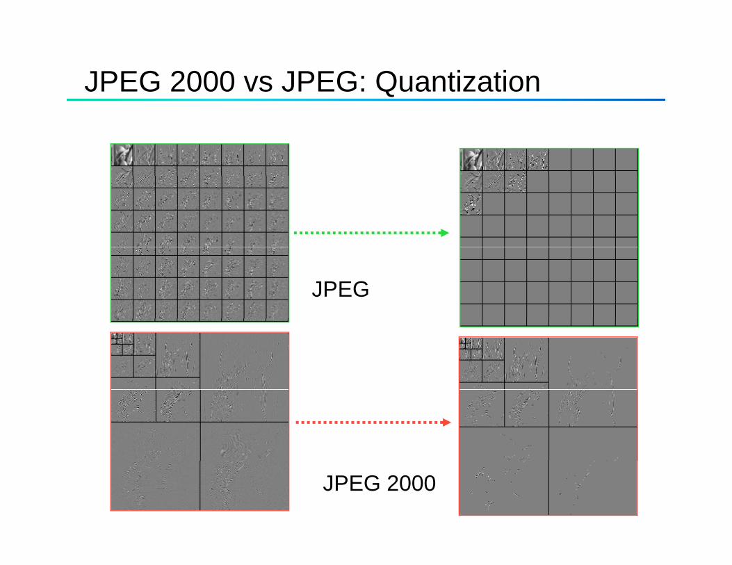
JPEG 2000 vs JPEG: Quantization

JPEG

JPEG 2000

JPEG 2000 vs JPEG: 0.3 bpp

JPEG

JPEG 2000

JPEG 2000 vs JPEG: Bitrate=0.3 bpp

MSE=150 MSE=73PSNR=26.2 db PSNR=29.5 db

JPEG 2000 vs JPEG: Bitrate=0.2 bpp

MSE=320 MSE=113MSE=320 MSE=113

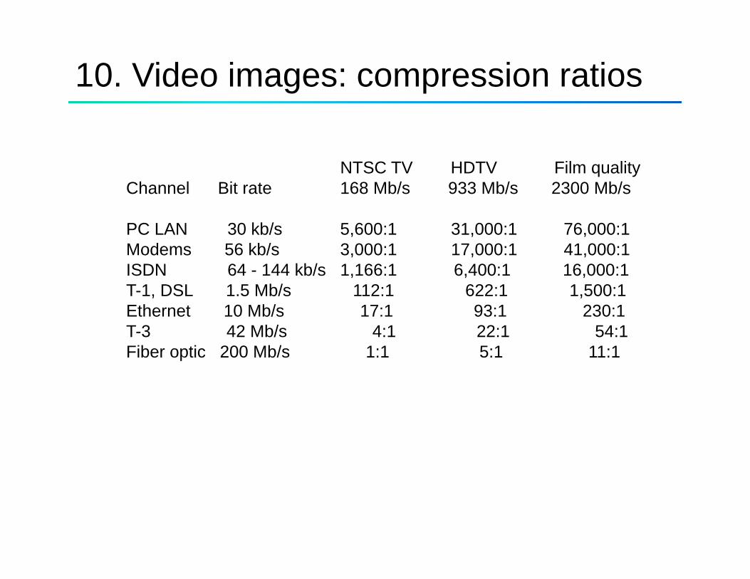
10. Video images: compression ratios

NTSC TV HDTV Film qualityChannel Bit rate 168 Mb/s 933 Mb/s 2300 Mb/s

PC LAN 30 kb/s 5,600:1 31,000:1 76,000:1Modems 56 kb/s 3 000:1 17 000:1 41 000:1Modems 56 kb/s 3,000:1 17,000:1 41,000:1ISDN 64 - 144 kb/s 1,166:1 6,400:1 16,000:1T-1, DSL 1.5 Mb/s 112:1 622:1 1,500:1Ethernet 10 Mb/s 17:1 93:1 230:1T 3 42 Mb/ 4 1 22 1 54 1T-3 42 Mb/s 4:1 22:1 54:1Fiber optic 200 Mb/s 1:1 5:1 11:1

Video Images and Still Images

• Video images are three-dimensional generalizationVideo images are three dimensional generalization of still images, where the third dimension is time

E h f f id b d b• Each frame of a video sequence can be compressed by any image compression algorithm

• Motion JPEG (M-JPEG): the images are separately coded by JPEG

Correlation

• Let’s take an advantage of the temporal correlations;Let s take an advantage of the temporal correlations; i.e. the fact that subsequent images resemble each other very much:

• Still Images : spatial correlation • Video Images: spatial and temporal correlation

MPEG-1

The MPEG algorithm relies on two basic techniquesg q• Block based motion compensation• DCT based compression

MPEGs

• MPEG-1 (1992): VideoCD • MPEG-2 (1994): DVD, digital TV, SVCDMPEG 2 (1994): DVD, digital TV, SVCD

* about 50:1 compression, typically 3-10 Mbps • MPEG-3: was abandoned

G ( ) ( f )• MPEG-4 (1999+): DivX (starting from Version 5) * designed specially for low-bandwidthMPEG 7 (>1998):• MPEG-7 (>1998): * searching and indexing of a/v data, using DescriptionToolsTools

MPEG-1: Blocks

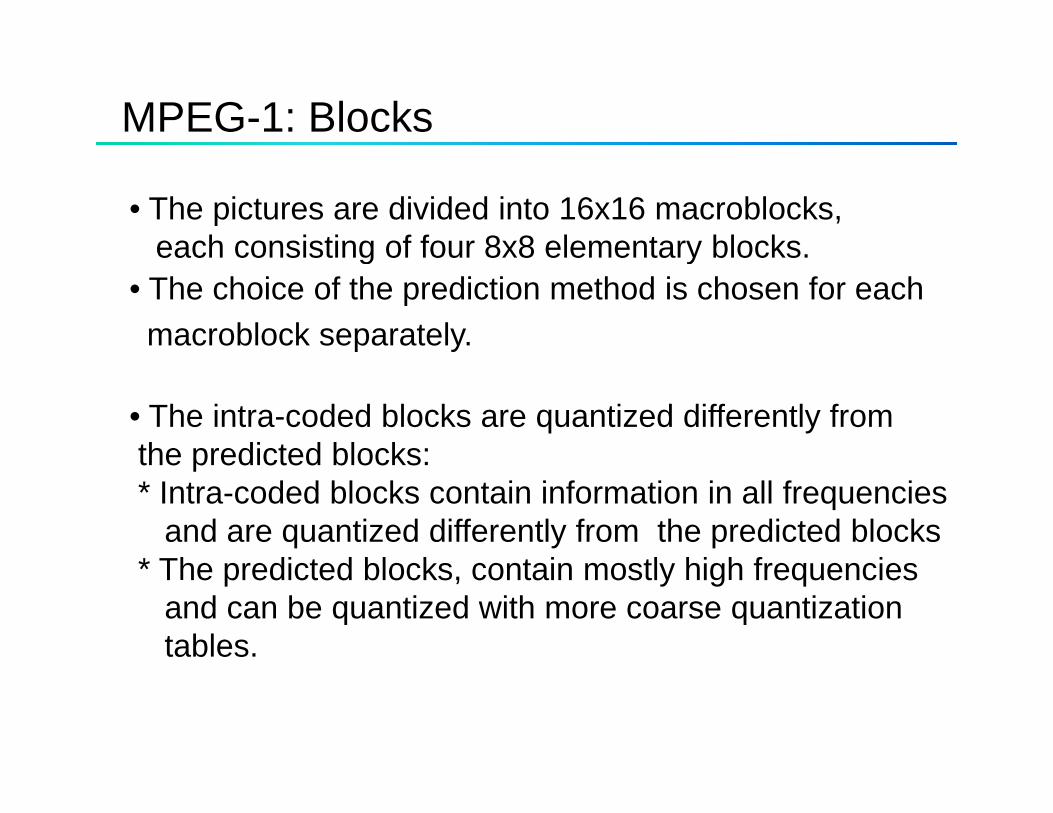
• The pictures are divided into 16x16 macroblocks, each consisting of four 8x8 elementary blockseach consisting of four 8x8 elementary blocks.

• The choice of the prediction method is chosen for eachmacroblock separately.

• The intra-coded blocks are quantized differently from the predicted blocks:the predicted blocks: * Intra-coded blocks contain information in all frequencies

and are quantized differently from the predicted blocks * Th di t d bl k t i tl hi h f i* The predicted blocks, contain mostly high frequencies

and can be quantized with more coarse quantization tables.

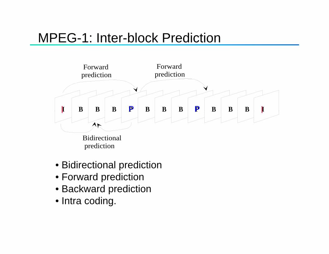
MPEG-1: Inter-block Prediction

Forwardprediction

Forwardprediction

I B B B P B B B P B B B II IP PI B B B P B B B

Bidirectional

P B B B II IP P

prediction

• Bidirectional predictionForward prediction• Forward prediction

• Backward prediction• Intra coding.

MPEG-1: Predictions schemes

I: Intra pictures are coded as still images by DCT. p g yP: Predicted pictures are coded with reference to a past

picture. The difference between the prediction and the original picture is then compressed by DCT.

B: Bidirectional pictures, the prediction can be made both t t d f t f Bidi ti l i tto a past and a future frame. Bidirectional pictures are never used as reference.

Forward Forward

I B B B P B B B

Forwardprediction

P B B B I

Forwardprediction

Bidirectional prediction

Motion estimation and compensation

• The prediction block in the reference frame is not necessarily in the same coordinates than the block innecessarily in the same coordinates than the block inthe current frame.

• Because of motion in the image sequence, the most suitable predictor for the current block may exist anywhere in the reference frame.

• The motion estimation specifies where the best prediction (best match) is found. M ti ti i t f l l ti th diff• Motion compensation consists of calculating the difference between the reference and the current block.

Motion estimation: 1

• Exhaustive search block matchingg

Slow!

Motion estimation: 2

• Hierarchical block matchingg

Compression ratios

NTSC TV HDTV Film qualityChannel Bit rate 168 Mb/s 933 Mb/s 2300 Mb/s

PC LAN 30 kb/s 5,600:1 31,000:1 76,000:1Modems 56 kb/s 3,000:1 17,000:1 41,000:1ISDN 64 - 144 kb/s 1,166:1 6,400:1 16,000:1, , ,T-1, DSL 1.5 Mb/s 112:1 622:1 1,500:1Ethernet 10 Mb/s 17:1 93:1 230:1T-3 42 Mb/s 4:1 22:1 54:1Fiber optic 200 Mb/s 1:1 5:1 11:1Fiber optic 200 Mb/s 1:1 5:1 11:1

Object-based coding

VOP- Video object planeVOL- Video object layer

Video content analysis

• Bring video sequence into chunks, each with consistent content: shotsconsistent content: shots

• Group similar shots into scenes• Describe connections between scenes• Associate shots/scenes with semantics for future query