Lossy Image Compression Methods - University of Washington

1

CSEP 590

Data CompressionAutumn 2007

Scalar Quantization

Vector Quantization

CSEP 590 - Lecture 8 - Autumn 2007 2

Lossy Image Compression Methods

• DCT Compression

– JPEG

• Scalar quantization (SQ).

• Vector quantization (VQ).

• Wavelet Compression

– SPIHT

– GTW

– EBCOT

– JPEG 2000


Scalar Quantization

0

1

n-1

.

.

.

codebook

i

index of a codeword

0

1

n-1

.

.

.

codebook

source image

decoded image


Scalar Quantization Strategies

• Build a codebook with a training set. Encode

and decode with fixed codebook.

– Most common use of quantization

• Build a codebook for each image. Transmit

the codebook with the image.

• Training can be slow.


Distortion

• Let the image be pixels x1, x2, … xT.

• Define index(x) to be the index transmitted on

input x.

• Define c(j) to be the codeword indexed by j.

T

DMSE

n)(Distortio))c(index(x(xD 2i

T

1i i

=

−=∑ =


Uniform Quantization Example

• 512 x 512 image with 8 bits per pixel.

• 8 codewords

0 31 63 95 127 159 191 223 255

Codebook

239207175143111794716

76543210IndexCodeword

boundary codeword

2


Uniform Quantization Example

Encoder

111110101100011010001000

224-255192-223160-191128-15996-12764-9532-630-31inputcode

239207175143111794716

111110101100011010001000

Decoder

codeoutput

Bit rate = 3 bits per pixelCompression ratio = 8/3 = 2.67


Example

• [0,100) with 5 symbols

• Q = 20

M

50201/2)(220

502

30201/2)(120

301

10201/2)(020

100

Decode Encode

=⋅+

=

=⋅+

=

=⋅+

=

0 20 40 60 80 100

0 1 2 3 4


Alternative Uniform Quantization

Calculation with Push to Zero

• Range = [min, max)

• Target is S symbols

• Choose Q = (max – min)/S

• Encode x

• Decode s

+= 1/2Q

xs

Q sx'=


Example

• [0,90) with 5 symbols

• Q = 20

M

402021/220

49.992

202011/220

29.991

02001/220

9.990

Decode Encode

=⋅

+=

=⋅

+=

=⋅

+=0 10 30 50 70 90

0 1 2 3 4


Improving Bit Rate

0 31 63 95 127 159 191 223 255

qj = the probability that a pixel is coded to index jPotential average bit rate is entropy.

Frequency of pixel values

)q

1(logqH

j

2

7

0j

j∑=

=


Example

• 512 x 512 image = 216,144 pixels

9,14418,00010,00010,00010,00090,000100,00025,000

224-255192-223160-191128-15996-12764-9532-630-31

index

inputfrequency

0 1 2 3 4 5 6 7

35 4

6

2

1

0

7

Huffman Tree ABR= (100000 x 1+90000 x 2 +43000 x 4 +39144 x 5)/216144

=2.997Arithmetic coding should workbetter.

3


Improving Distortion

• Choose the codeword as a weighted average

0 31 63 95 127 159 191 223 255

Let px be the probability that a pixel has value x.Let [Lj,Rj) be the input interval for index j. c(j) is the codeword indexed j

)pxround(c(j)jj RxL

x∑<≤

⋅=


Example

010203040100100100

15141312111098pixel valuefrequency

16000311021201130 Distortion Old

1000041032021301140 DistortionNew

11 Codeword Old

10 )400

0151014201330124011100101009 1008round( CodewordNew

222

2222

=⋅+⋅+⋅=

=⋅+⋅+⋅+⋅=

=

=⋅+⋅+⋅+⋅+⋅+⋅+⋅+⋅=

All pixels have the same index.


An Extreme Case

0 31 63 95 127 159 191 223 255


Only two codewords are ever used!!


Non-uniform Scalar Quantization

0 255


codewordboundary between codewords


Lloyd Algorithm

• Lloyd (1957)

• Creates an optimized codebook of size n.

• Let px be the probability of pixel value x. – Probabilities might come from a training set

• Given codewords c(0),c(1),...,c(n-1) and pixel x let index(x) be the index of the closest code word to x.

• Expected distortion is

• Goal of the Lloyd algorithm is to find the codewordsthat minimize distortion.

• Lloyd finds a local minimum by an iteration process.

2

xx ))c(index(x)(xpD −=∑


Lloyd Algorithm

Choose a small error tolerance ε > 0.Choose start codewords c(0),c(1),...,c(n-1)Compute X(j) := {x : x is a pixel value closest to c(j)}Compute distortion D for c(0),c(1),...,c(n-1) Repeat

Compute new codewords

Compute X’(j) = {x : x is a pixel value closest to c’(j)}Compute distortion D’ for c’(0),c’(1),...,c’(n-1)

if |(D – D’)/D| < ε then quitelse c := c’; X := X’, D := D’

End{repeat}

)/ppxround(:(j)c'X(j)x

X(j)x∑∈

⋅=

4


Example

010203040100100100


Initially c(0) = 2 and c(1) = 5

57)/60)06105204round((30(1)c'

13)/340)40210011000round((100(0)c'

580D(1)D(0) D

40140D(1) 540; 21001140 D(0)

[4,7]X(1) [0,3], X(0)222

=⋅+⋅+⋅+⋅==⋅+⋅+⋅+⋅=

=+==⋅==⋅+⋅=

==


Example

010203040100100100


D':D;X':X;c':c

.31400)/580(580)/DD'(D

400(1)D'(0)D'D'

200240140 (1)D'

200 1200 (0)D'

[3,7](1)X' [0,2]; (0)X'

5(1)c' 1;(0)c'

22

2

====−=−

=+==⋅+⋅=

=⋅=

====


Example

010203040100100100


47)/100)06105204303round((40(1)c'

12)/300)10011000round((100(0)c'

400D

[3,7]X(1) [0,2]; X(0)

5c(1) 1;c(0)

=⋅+⋅+⋅+⋅+⋅==⋅+⋅+⋅=

===

==


Example

010203040100100100


D':D;X':X;c':c

.17300)/580(400)/DD'(D

300(1)D'(0)D'D'

100210160 (1)D'

200 1200 (0)D'

[3,7](1)X' [0,2]; (0)X'

4(1)c' 1;(0)c'

22

2

====−=−

=+==⋅+⋅=

=⋅=

====


Example

010203040100100100


47)/100)06105204303round((40(1)c'

12)/300)10011000round((100(0)c'

400D

[3,7]X(1) [0,2]; X(0)

4c(1) 1;c(0)

=⋅+⋅+⋅+⋅+⋅==⋅+⋅+⋅=

===

==


Example

010203040100100100


4.c(1) and 1 c(0) codeword withExit

0300)/580(300)/DD'(D

300(1)D'(0)D'D'

100210160 (1)D'

200 1200 (0)D'

[3,7](1)X' [0,2]; (0)X'

4(1)c' 1;(0)c'

22

2

===−=−

=+==⋅+⋅=

=⋅=

====

5


Scalar Quantization Notes

• Useful for analog to digital conversion.

• Useful for estimating a large set of values with a small set of values.

• With entropy coding yields good lossy compression.

• Lloyd algorithm works very well in practice, but can take many iterations.– For n codewords should use about 20n size

representative training set.

– imagine 1024 codewords.


Vector Quantization

1

2

n

.

.

.

source imagecodebook

1

2

n

.

.

.

codebook

i

index of nearest codeword

decoded image


Vectors

• An a x b block can be considered to be a vector of dimension ab.

• Nearest means in terms of Euclidian distance or Euclidian squared distance. Both equivalent.

• Squared distance is easier to calculate.

w xzyblock = (w,x,y,z) vector

2

21

2

21

2

21

2

21

2

21

2

21

2

21

2

21

)z(z)y(y)x(x)w(w Distance Squared

)z(z)y(y)x(x)w(wDistance

−+−+−+−=

−+−+−+−=


Vector Quantization Facts

• The image is partitioned into a x b blocks.

• The codebook has n representative a x b blocks called codewords, each with an index.

• Compression with fixed length codes is

• Example: a = b = 4 and n = 1,024

– compression is 10/16 = .63 bpp

– compression ratio is 8 : .63 = 12.8 : 1

• Better compression with entropy coding of indices

ab

nlog2 bpp


Examples

4 x 4 blocks.63 bpp

4 x 8 blocks.31 bpp

8 x 8 blocks.16 bpp

Codebook size = 1,024


Scalar vs. Vector

• Pixels within a block are correlated.

– This tends to minimize the number of codewordsneeded to represent the vectors well.

• More flexibility.

– Different size blocks

– Different size codebooks

6


Encoding and Decoding

• Encoding:

– Scan the a x b blocks of the image. For each block find the nearest codeword in the codebook and output its index.

– Nearest neighbor search.

• Decoding:

– For each index output the codeword with that index into the destination image.

– Table lookup.


The Codebook

• Both encoder and decoder must have the

same codebook.

• The codebook must be useful for many

images and be stored someplace.

• The codebook must be designed properly to

be effective.

• Design requires a representative training set.

• These are major drawbacks to VQ.


Codebook Design Problem

• Input: A training set X of vectors of dimension

d and a number n. (d = a x b and n is number

of codewords)

• Ouput: n codewords c(0), c(1),...,c(n-1) that

minimize the distortion.

where index(x) is the index of the nearest

codeword to x.

∑∈

−=Xx

2)c(index(x)xD

2

1d

2

1

2

0

2

1d10 xxx)x,x,(x −− +++= LL squared norm

sum of squared distances


GLA

• The Generalized Lloyd Algorithm (GLA)

extends the Lloyd algorithm for scalars.

– Also called LBG after inventors Linde, Buzo, Gray (1980)

• It can be very slow for large training sets.


GLA

Choose a training set X and small error tolerance ε > 0.Choose start codewords c(0),c(1),...,c(n-1)Compute X(j) := {x : x is a vector in X closest to c(j)}Compute distortion D for c(0),c(1),...,c(n-1) Repeat

Compute new codewords

Compute X’(j) = {x : x is a vector in X closest to c’(j)}Compute distortion D’ for c’(0),c’(1),...,c’(n-1)

if |(D – D’)/D| < ε then quitelse c := c’; X := X’, D := D’

End{repeat}

)x|X(j)|

1round(:(j)c'

X(j)x

∑∈

= (centroid)


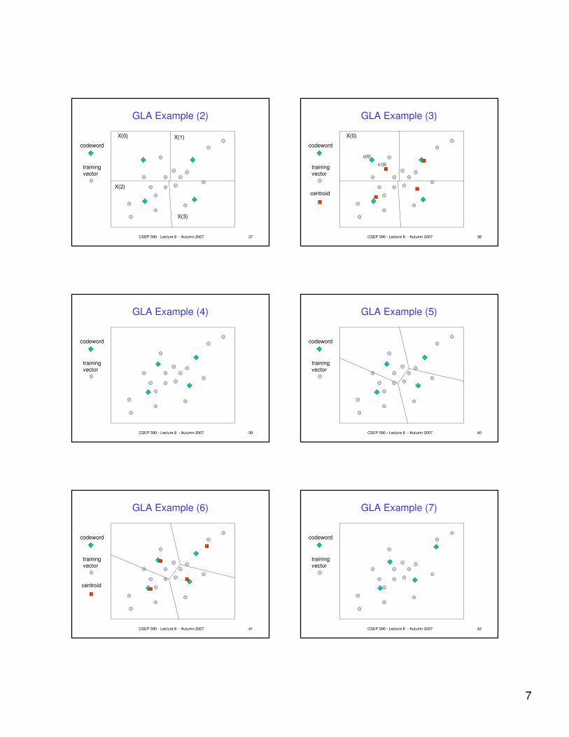
GLA Example (1)

codeword

trainingvector

c(0)

c(2) c(3)

c(1)

7


GLA Example (2)

codeword

trainingvector

X(0)

X(3)

X(2)

X(1)


GLA Example (3)

codeword

trainingvector

centroid

X(0)

c(0)

c’(0)


GLA Example (4)

codeword

trainingvector


GLA Example (5)

codeword

trainingvector


GLA Example (6)

codeword

trainingvector

centroid


GLA Example (7)

codeword

trainingvector

8


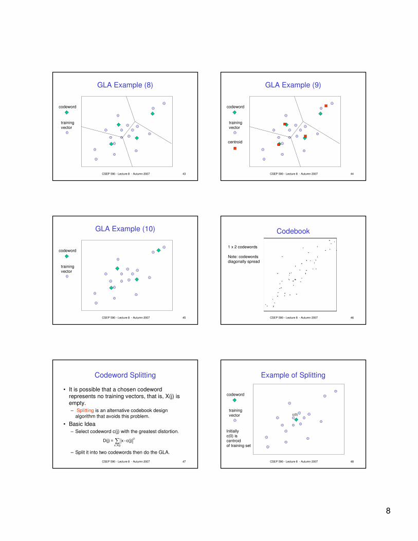
GLA Example (8)

codeword

trainingvector


GLA Example (9)

codeword

trainingvector

centroid


GLA Example (10)

codeword

trainingvector


Codebook

1 x 2 codewords

Note: codewordsdiagonally spread


Codeword Splitting

• It is possible that a chosen codeword

represents no training vectors, that is, X(j) is

empty.

– Splitting is an alternative codebook design algorithm that avoids this problem.

• Basic Idea

– Select codeword c(j) with the greatest distortion.

– Split it into two codewords then do the GLA.

∑∈

=X(j)x

2c(j)-xD(j)


Example of Splitting

codeword

trainingvector c(0)

Initiallyc(0) is centroidof training set

9



codeword

trainingvector c(0) c(1)

Split

c(1) = c(0) + ε



codeword

trainingvector

c(0)

c(1)

Apply GLA



codeword

trainingvector

c(0)

c(1)

c(0) has max

distortion sosplit it.

c(2)

X(0)

X(1)



codeword

trainingvector

c(0)

c(1)

Apply GLA

c(2)

X(0)

X(1)

X(2)



codeword

trainingvector

c(0)

c(1)

c(2) has max

distortion sosplit it

c(2)

c(3)

X(0)

X(1)

X(2)



codeword

trainingvector

c(0)

c(1)

c(2)

X(0)

X(1)

c(3)

X(2)

X(3)

10


GLA Advice

• Time per iteration is dominated by the

partitioning step, which is m nearest neighbor

searches where m is the training set size.

– Average time per iteration O(m log n) assuming d is small.

• Training set size.

– Training set should be at least 20 training vectors per code word to get reasonable performance.

– Too small a training set results in “over training”.

• Number of iterations can be large.


Encoding

• Naive method.– For each input block, search the entire codebook

to find the closest codeword.

– Time O(T n) where n is the size of the codebook and T is the number of blocks in the image.

– Example: n = 1024, T = 256 x 256 = 65,536 (2 x 2 blocks for a 512 x 512 image)nT = 1024 x 65536 = 226 ≈ 67 million distance calculations.

• Faster methods are known for doing “Full Search VQ”. For example, k-d trees.– Time O(T log n)


VQ Encoding is Nearest Neighbor

Search

• Given an input vector, find the closest

codeword in the codebook and output its

index.

• Closest is measured in squared Euclidian

distance.

• For two vectors (w1,x1,y1,z1) and (w2,x2,y2,z2).

2

21

2

21

2

21

2

21 )z(z)y(y)x(x)w(w Distance Squared −+−+−+−=


k-d Tree

• Jon Bentley, 1975

• Tree used to store spatial data.

– Nearest neighbor search.

– Range queries.

– Fast look-up

• k-d tree are guaranteed log2 n depth where n

is the number of points in the set.

– Traditionally, k-d trees store points in d-dimensional space which are equivalent to vectors in d-dimensional space.


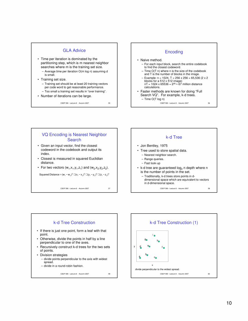
k-d Tree Construction

• If there is just one point, form a leaf with that point.

• Otherwise, divide the points in half by a line perpendicular to one of the axes.

• Recursively construct k-d trees for the two sets of points.

• Division strategies– divide points perpendicular to the axis with widest

spread.

– divide in a round-robin fashion.


x

y

k-d Tree Construction (1)

ab

f

c

gh

ed

i

divide perpendicular to the widest spread.

11


y


x

ab

c

gh

ed

i s1

s1

x

f


y


x

ab

c

gh

ed

i s1

s2y

s1

s2

x

f


y


x

ab

c

gh

ed

i s1

s2y

s3x

s1

s2

s3

x

f


y


x

ab

c

gh

ed

i s1

s2y

s3x

s1

s2

s3

a

x

f


y


x

ab

c

gh

ed

i s1

s2y

s3x

s1

s2

s3

a b

x

f


y


x

ab

c

gh

ed

i s1

s2y

s3x

s4y

s1

s2

s3

s4

a b

x

f

12


y


x

ab

c

gh

ed

i s1

s2y

s3x

s4y

s5x

s1

s2

s3

s4

s5

a b

x

f


y


x

ab

c

gh

ed

i s1

s2y

s3x

s4y

s5x

s1

s2

s3

s4

s5

a b

dx

f


y


x

ab

c

gh

ed

i s1

s2y

s3x

s4y

s5x

s1

s2

s3

s4

s5

a b

d ex

f


y


x

ab

c

gh

ed

i s1

s2y

s3x

s4y

s5x

s1

s2

s3

s4

s5

a b

d e

g

x

f


y


x

ab

c

gh

ed

i s1

s2y y

s6

s3x

s4y

s5x

s1

s2

s3

s4

s5

s6

a b

d e

g

x

f


y


x

ab

c

gh

ed

i s1

s2y y

s6

s3x

s4y

s7y

s5x

s1

s2

s3

s4

s5

s6

s7

a b

d e

g

x

f

13


y


x

ab

c

gh

ed

i s1

s2y y

s6

s3x

s4y

s7y

s5x

s1

s2

s3

s4

s5

s6

s7

a b

d e

g c

x

f


y


x

ab

c

gh

ed

i s1

s2y y

s6

s3x

s4y

s7y

s5x

s1

s2

s3

s4

s5

s6

s7

a b

d e

g c f

x

f


y


x

ab

c

gh

ed

i s1

s2y y

s6

s3x

s4y

s7y

s8y

s5x

s1

s2

s3

s4

s5

s6

s7

s8

a b

d e

g c f

x

f


y


x

ab

c

gh

ed

i s1

s2y y

s6

s3x

s4y

s7y

s8y

s5x

s1

s2

s3

s4

s5

s6

s7

s8

a b

d e

g c f h

x

f


y


x

ab

c

gh

ed

i s1

s2y y

s6

s3x

s4y

s7y

s8y

s5x

s1

s2

s3

s4

s5

s6

s7

s8

a b

d e

g c f h i

x

f


k-d Tree Construction Complexity

• First sort the points in each dimension.

– O(dn log n) time and dn storage.

– These are stored in A[1..d,1..n]

• Finding the widest spread and equally

dividing into two subsets can be done in

O(dn) time.

• Constructing the k-d tree can be done in

O(dn log n) and dn storage

14


k-d Tree Codebook Organization

2-d vectors(x,y)

x

y


Node Structure for k-d Trees

• A node has 5 fields

– axis (splitting axis)

– value (splitting value)

– left (left subtree)

– right (right subtree)

– point (holds a point if left and right children are null)


k-d Tree Nearest Neighbor Search

NNS(q, root, p, infinity)initial call

NNS(q: point, n: node, p: ref point w: ref distance)if n.left = n.right = null then {leaf case}

w’ := ||q - n.point||;

if w’ < w then w := w’; p := n.point;else

if w = infinity thenif q(n.axis) < n.value then

NNS(q, n.left, p, w);if q(n.axis) + w > n.value then NNS(q, n.right, p, w);

else NNS(q, n.right, p, w);if q(n.axis) - w < n.value then NNS(q, n.left, p, w)

else {w is finite}if q(n.axis) - w < n.value then NNS(q, n.left, p, w)if q(n.axis) + w > n.value then NNS(q, n.right, p, w);


Explanation

n.value q(n.axis)

q(n.axis) – w < n.valuemeans the circle overlapsthe left subtree.

w

searchleft nearest

codeword

query

q(n.axis) n.value

q(n.axis) + w > n.valuemeans the circle overlapsthe right subtree.

w

searchright


y

k-d Tree NNS (1)

x

ab

c

gh

ed

i s1

s2y y

s6

s3x

s4y

s7y

s8y

s5x

s1

s2

s3

s4

s5

s6

s7

s8

a b

d e

g c f h i

x

f

query point


y

k-d Tree NNS (2)

x

ab

c

gh

ed

i s1

s2y y

s6

s3x

s4y

s7y

s8y

s5x

s1

s2

s3

s4

s5

s6

s7

s8

a b

d e

g c f h i

x

f

query point

15


y

k-d Tree NNS (3)

x

ab

c

gh

ed

i s1

s2y y

s6

s3x

s4y

s7y

s8y

s5x

s1

s2

s3

s4

s5

s6

s7

s8

a b

d e

g c f h i

x

f

query point


y

k-d Tree NNS (4)

x

ab

c

gh

ed

i s1

s2y y

s6

s3x

s4y

s7y

s8y

s5x

s1

s2

s3

s4

s5

s6

s7

s8

a b

d e

g c f h i

x

f

query point

w


y

k-d Tree NNS (5)

x

ab

c

gh

ed

i s1

s2y y

s6

s3x

s4y

s7y

s8y

s5x

s1

s2

s3

s4

s5

s6

s7

s8

a b

d e

c f h i

x

f

query point

w

g


y

k-d Tree NNS (6)

x

ab

c

gh

ed

i s1

s2y y

s6

s3x

s4y

s7y

s8y

s5x

s1

s2

s3

s4

s5

s6

s7

s8

a b

d e

c f h i

x

f

query point

w

g


y

k-d Tree NNS (7)

x

ab

c

gh

ed

i s1

s2y y

s6

s3x

s4y

s7y

s8y

s5x

s1

s2

s3

s4

s5

s6

s7

s8

a b

d e

c f h i

x

f

query point

w

g


y

k-d Tree NNS (8)

x

ab

c

gh

ed

i s1

s2y y

s6

s3x

s4y

s7y

s8y

s5x

s1

s2

s3

s4

s5

s6

s7

s8

a b

d e

c f h i

x

f

query point

w

g

16


e

y

k-d Tree NNS (9)

x

ab

c

gh

ed

i s1

s2y y

s6

s3x

s4y

s7y

s8y

s5x

s1

s2

s3

s4

s5

s6

s7

s8

a b

d

c f h i

x

f

query point

w

g


y

k-d Tree NNS (10)

x

ab

c

gh

ed

i s1

s2y y

s6

s3x

s4y

s7y

s8y

s5x

s1

s2

s3

s4

s5

s6

s7

s8

a b

d

c f h i

x

f

query point

w

e

g


y

k-d Tree NNS (11)

x

ab

c

gh

ed

i s1

s2y y

s6

s3x

s4y

s7y

s8y

s5x

s1

s2

s3

s4

s5

s6

s7

s8

a b

d

c f h i

x

f

query point

w

e

g


y

k-d Tree NNS (12)

x

ab

c

gh

ed

i s1

s2y y

s6

s3x

s4y

s7y

s8y

s5x

s1

s2

s3

s4

s5

s6

s7

s8

a b

d

c f h i

x

f

query point

w

e

g


y

k-d Tree NNS (13)

x

ab

c

gh

ed

i s1

s2y y

s6

s3x

s4y

s7y

s8y

s5x

s1

s2

s3

s4

s5

s6

s7

s8

a b

d

c f h i

x

f

query point

w

e

g


y

k-d Tree NNS (14)

x

ab

c

gh

ed

i s1

s2y y

s6

s3x

s4y

s7y

s8y

s5x

s1

s2

s3

s4

s5

s6

s7

s8

a b

d

c f h i

x

f

query point

w

e

g

17


y

k-d Tree NNS (15)

x

ab

c

gh

ed

i s1

s2y y

s6

s3x

s4y

s7y

s8y

s5x

s1

s2

s3

s4

s5

s6

s7

s8

a b

d

c f h i

x

f

query point

w

e

g


y

k-d Tree NNS (16)

x

ab

c

gh

ed

i s1

s2y y

s6

s3x

s4y

s7y

s8y

s5x

s1

s2

s3

s4

s5

s6

s7

s8

a b

d

c f h i

x

f

query point

w

e

g


y

k-d Tree NNS (17)

x

ab

c

gh

ed

i s1

s2y y

s6

s3x

s4y

s7y

s8y

s5x

s1

s2

s3

s4

s5

s6

s7

s8

a b

d

c f h i

x

f

query point

w

e

g


y

k-d Tree NNS (18)

x

ab

c

gh

ed

i s1

s2y y

s6

s3x

s4y

s7y

s8y

s5x

s1

s2

s3

s4

s5

s6

s7

s8

a b

d

c f h i

x

f

query point

w

e

g


y

k-d Tree NNS (19)

x

ab

c

gh

ed

i s1

s2y y

s6

s3x

s4y

s7y

s8y

s5x

s1

s2

s3

s4

s5

s6

s7

s8

a b

d

c f h i

x

f

query point

w

e

g


y

k-d Tree NNS (20)

x

ab

c

gh

ed

i s1

s2y y

s6

s3x

s4y

s7y

s8y

s5x

s1

s2

s3

s4

s5

s6

s7

s8

a b

d

c f h i

x

f

query point

w

e

g

18


y

k-d Tree NNS (21)

x

ab

c

gh

ed

i s1

s2y y

s6

s3x

s4y

s7y

s8y

s5x

s1

s2

s3

s4

s5

s6

s7

s8

a b

d

c f h i

x

f

query point

w

e

g


Notes on k-d Tree NNS

• Has been shown to run in O(log n) average

time per search in a reasonable model.

(Assume d a constant)

• For VQ it appears that O(log n) is correct.

• Storage for the k-d tree is O(n).

• Preprocessing time is O(n log n) assuming d

is a constant.


Alternatives

• Orchard’s Algorithm (1991)

– Uses O(n2) storage but is very fast

• Annulus Algorithm

– Similar to Orchard but uses O(n) storage. Does many more distance calculations.

• PCP Principal Component Partitioning

– Zatloukal, Johnson, Ladner (1999)

– Similar to k-d trees

– Also very fast


Principal Component Partition


PCP Tree vs. k-d tree

PCP k-d


Comparison in Time per Search

0

1

2

3

4

5

6

7

4D 16D 64D

dimension

no

rma

lize

d t

ime

pe

r s

ea

rch

Orchard

k-d tree

PCP tree

4,096 codewords

19


Notes on VQ

• Works well in some applications.

– Requires training

• Has some interesting algorithms.

– Codebook design

– Nearest neighbor search

• Variable length codes for VQ.

– PTSVQ - pruned tree structured VQ (Chou, Lookabaugh and Gray, 1989)

– ECVQ - entropy constrained VQ (Chou, Lookabaugh and Gray, 1989)

Lossy Image Compression Methods - University of Washington

Documents

Transcript of Lossy Image Compression Methods - University of Washington