Lossy Compression III
49
LOSSY COMPRESSION III
-
Upload
rakesh-inani -
Category
Documents
-
view
228 -
download
0
Transcript of Lossy Compression III
8/10/2019 Lossy Compression III
http://slidepdf.com/reader/full/lossy-compression-iii 1/49
8/10/2019 Lossy Compression III
http://slidepdf.com/reader/full/lossy-compression-iii 2/49
Introduction Compression in all the lossy schemes is achieved
through quantization.
The process of representing a large – possiblyinfinite – set of values with a much smaller set iscalled quantization
Example: Source generates numbers between -10.0and +10.0 – Simple scheme is to represent eachoutput of the source with the integer value closer toit.
8/10/2019 Lossy Compression III
http://slidepdf.com/reader/full/lossy-compression-iii 3/49
Introduction
Two types of quantization
Scalar Quantization.
Vector Quantization.
The design of the quantizer has a significant
impact on the amount of compression (i.e.,rate) obtained and loss (distortion) incurred ina lossy compression scheme
8/10/2019 Lossy Compression III
http://slidepdf.com/reader/full/lossy-compression-iii 4/49
Scalar Quantization Many of the fundamental ideas of quantization and
compression are easily introduced in the simplecontext of scalar quantization.
Any real number x can be rounded off to the nearestinteger, say
Q(x) = round(x)
Maps the real line R (a continuous space) into adiscrete space.

8/10/2019 Lossy Compression III
http://slidepdf.com/reader/full/lossy-compression-iii 5/49
Scalar Quantization Quantizer: encoder mapping and decoder
mapping.
Encoder mapping The encoder divides the range of source into a number
of intervals
Each interval is represented by a distinct codeword
Decoder mapping For each received codeword, the decoder generates areconstruct value
8/10/2019 Lossy Compression III
http://slidepdf.com/reader/full/lossy-compression-iii 6/49
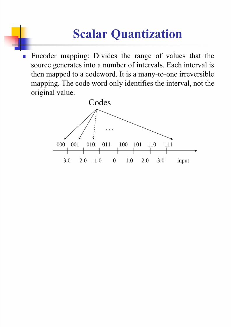
Scalar Quantization Encoder mapping: Divides the range of values that the
source generates into a number of intervals. Each interval is
then mapped to a codeword. It is a many-to-one irreversible
mapping. The code word only identifies the interval, not the
original value.
Codes
000 001 010 011 100 101 110 111
…
-3.0 -2.0 -1.0 0 1.0 2.0 3.0 input
8/10/2019 Lossy Compression III
http://slidepdf.com/reader/full/lossy-compression-iii 7/49
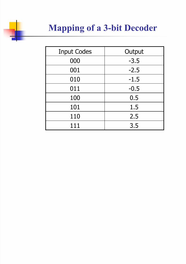
Scalar Quantization Decoder: Given the code word, the decoder
gives an estimated value that the source might
have generated.
Usually, it is the midpoint of the interval but a
more accurate estimate will depend on thedistribution of the values in the interval.
8/10/2019 Lossy Compression III
http://slidepdf.com/reader/full/lossy-compression-iii 8/49
Mapping of a 3-bit Decoder
Input Codes Output
000 -3.5
001 -2.5
010 -1.5
011 -0.5
100 0.5101 1.5
110 2.5
111 3.5
8/10/2019 Lossy Compression III
http://slidepdf.com/reader/full/lossy-compression-iii 9/49
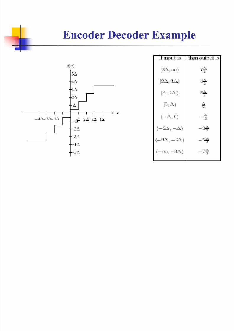
Encoder Decoder Example
8/10/2019 Lossy Compression III
http://slidepdf.com/reader/full/lossy-compression-iii 10/49
Scalar Quantization
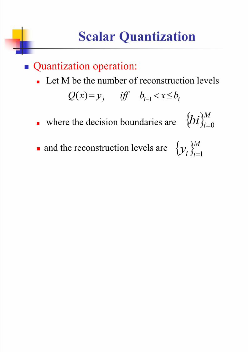
Quantization operation:
Let M be the number of reconstruction levels
where the decision boundaries are
and the reconstruction levels are
ii j b xbiff y xQ 1)(
M
ibi 0
M
ii y 1
8/10/2019 Lossy Compression III
http://slidepdf.com/reader/full/lossy-compression-iii 11/49
Scalar Quantization
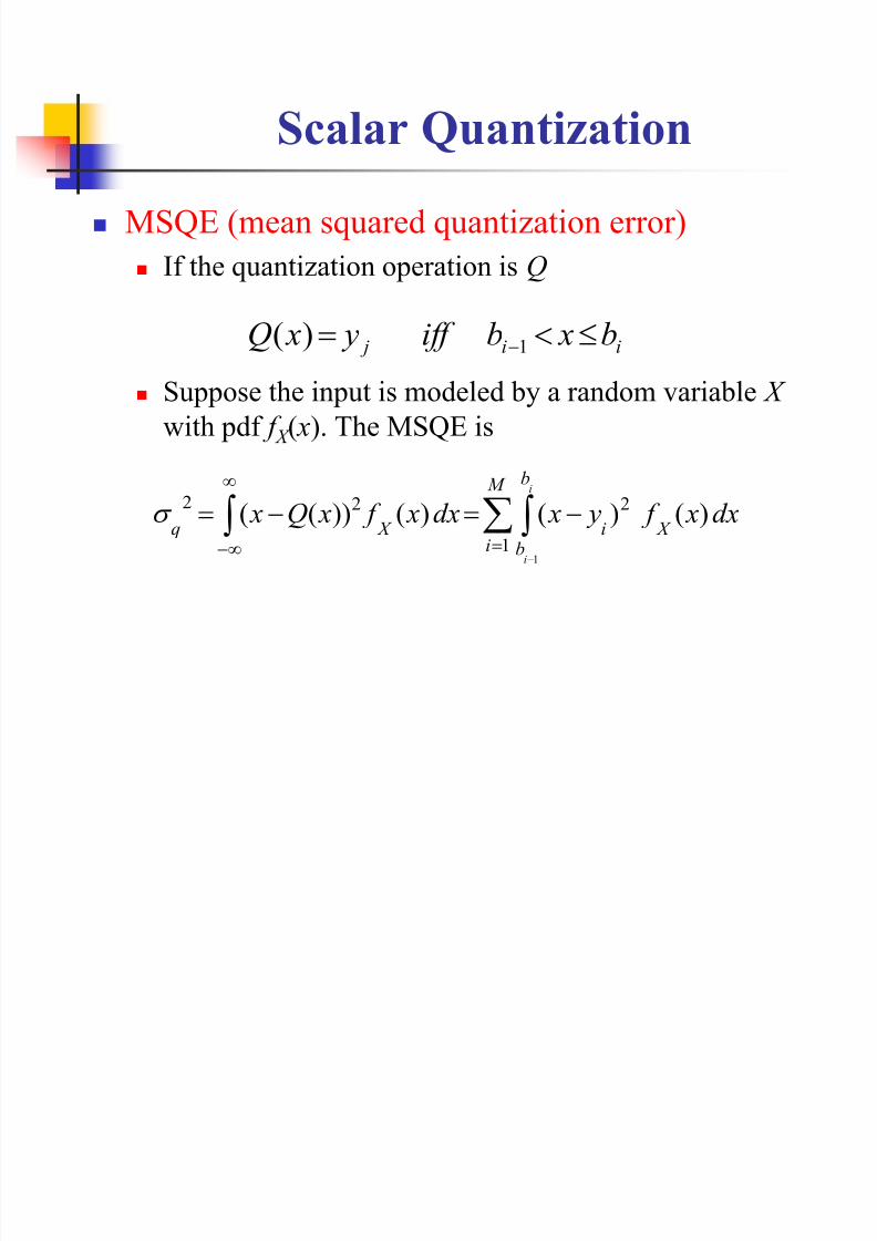
MSQE (mean squared quantization error)
If the quantization operation is Q
Suppose the input is modeled by a random variable X
with pdf f X ( x). The MSQE is
ii j b xbiff y xQ 1)(
dx x f y xdx x f xQ x X
M
i
b
bi X q
i
i
)()()())((1
222
1
8/10/2019 Lossy Compression III
http://slidepdf.com/reader/full/lossy-compression-iii 12/49
Scalar Quantization
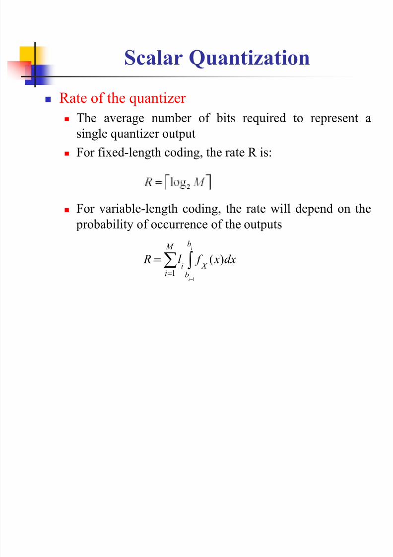
Rate of the quantizer
The average number of bits required to represent a
single quantizer output For fixed-length coding, the rate R is:
For variable-length coding, the rate will depend on the probability of occurrence of the outputs
M
i
b
b
X i
i
i
dx x f l R
1 1
)(
8/10/2019 Lossy Compression III
http://slidepdf.com/reader/full/lossy-compression-iii 13/49
8/10/2019 Lossy Compression III
http://slidepdf.com/reader/full/lossy-compression-iii 14/49
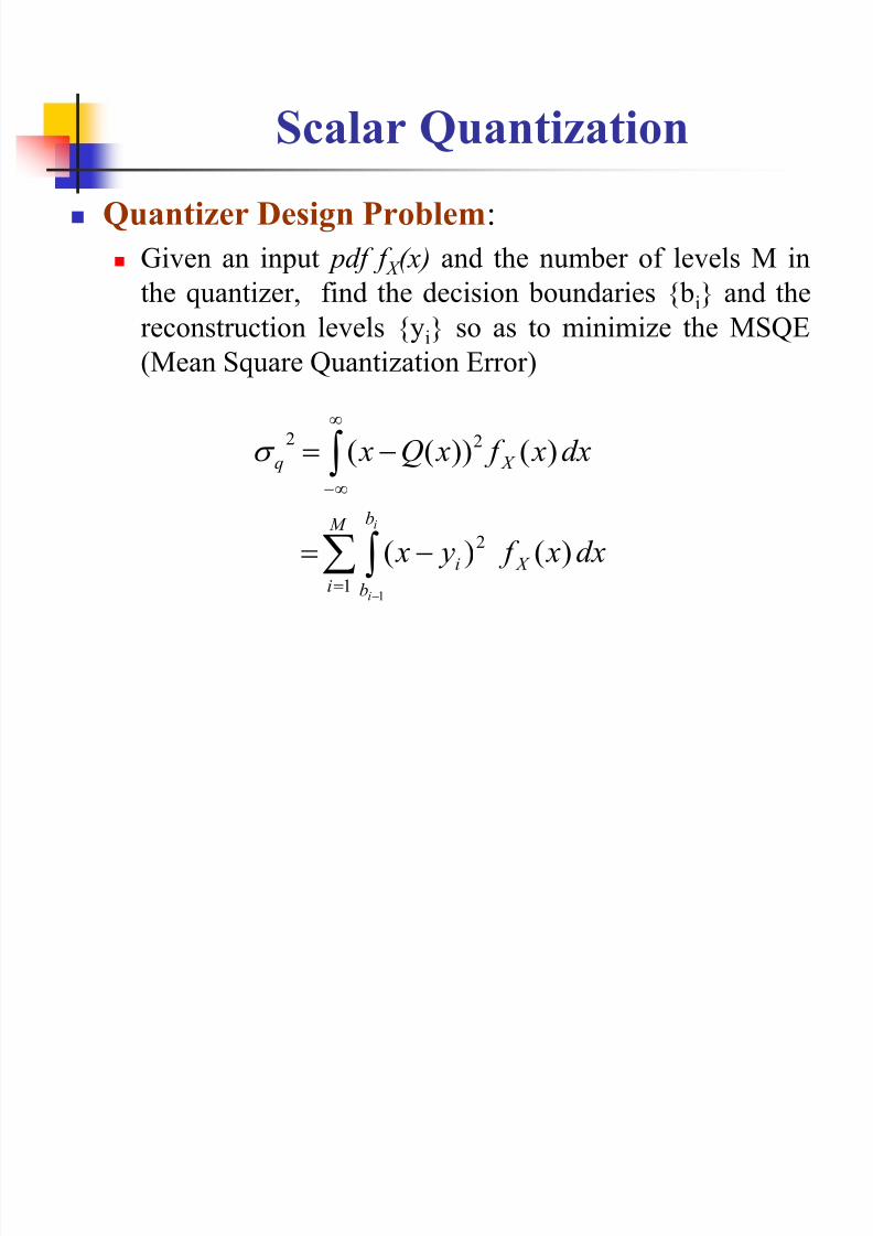
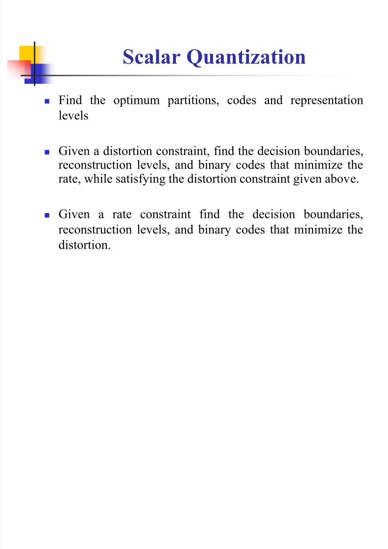
Scalar Quantization
Find the optimum partitions, codes and representation
levels
Given a distortion constraint, find the decision boundaries,reconstruction levels, and binary codes that minimize therate, while satisfying the distortion constraint given above.
Given a rate constraint find the decision boundaries,
reconstruction levels, and binary codes that minimize the
distortion.
8/10/2019 Lossy Compression III
http://slidepdf.com/reader/full/lossy-compression-iii 15/49
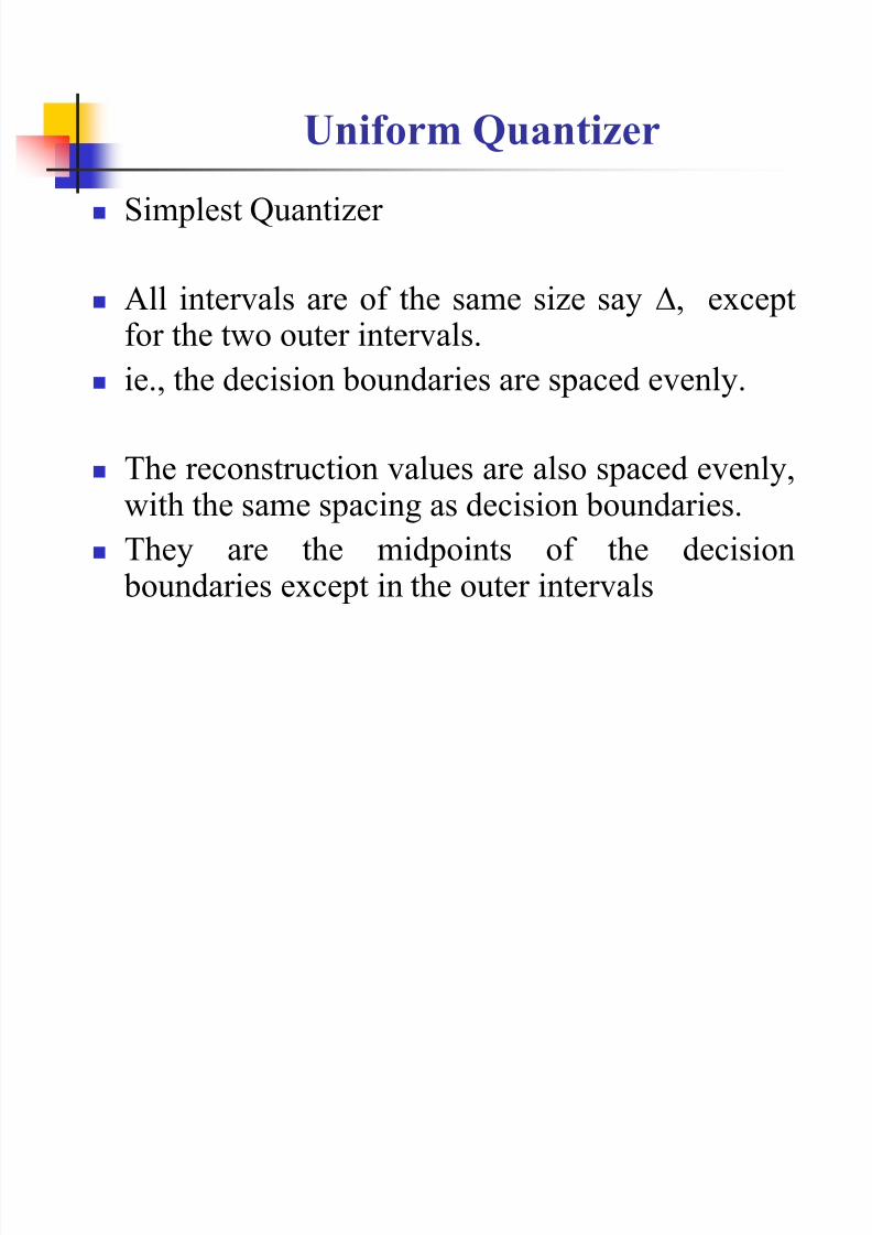
Uniform Quantizer
Simplest Quantizer
All intervals are of the same size say , exceptfor the two outer intervals.
ie., the decision boundaries are spaced evenly.
The reconstruction values are also spaced evenly,with the same spacing as decision boundaries.
They are the midpoints of the decision boundaries except in the outer intervals
8/10/2019 Lossy Compression III
http://slidepdf.com/reader/full/lossy-compression-iii 16/49
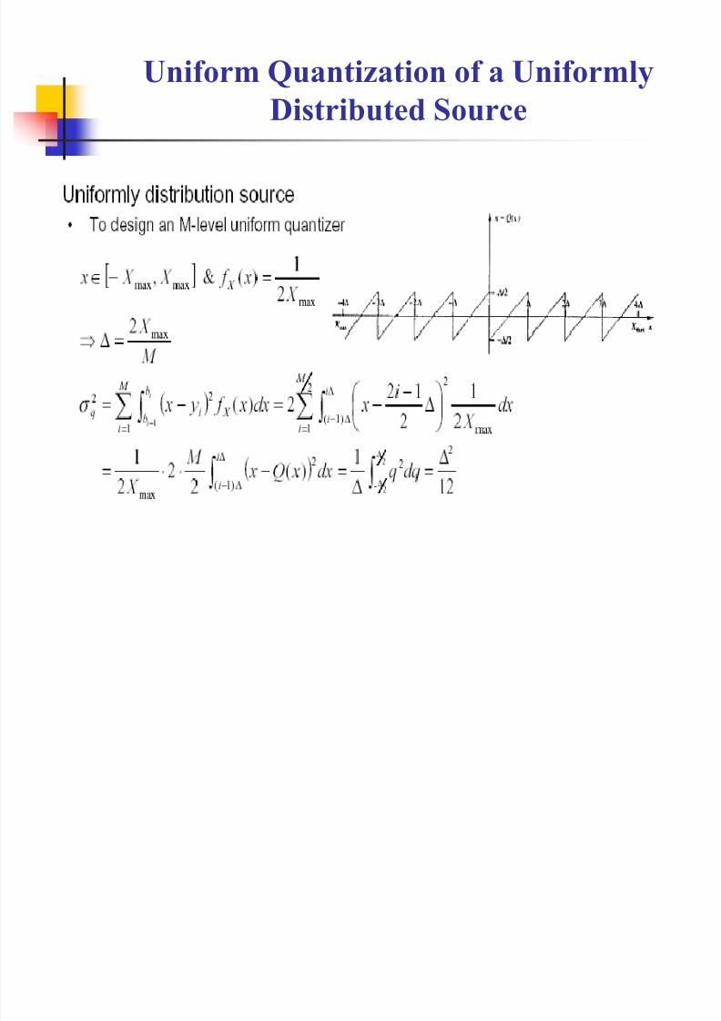
Uniform Quantization of a Uniformly
Distributed Source
8/10/2019 Lossy Compression III
http://slidepdf.com/reader/full/lossy-compression-iii 17/49
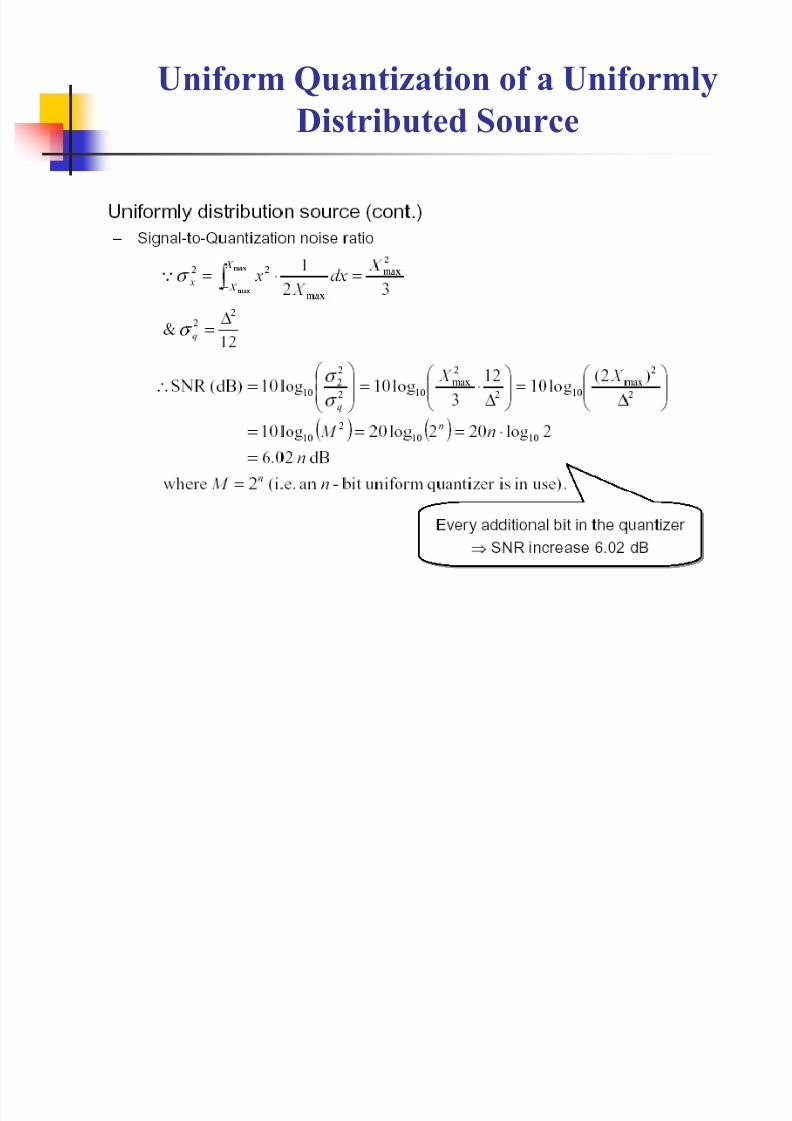
Uniform Quantization of a Uniformly
Distributed Source
8/10/2019 Lossy Compression III
http://slidepdf.com/reader/full/lossy-compression-iii 18/49
Uniform Quantization of a Uniformly
Distributed Source
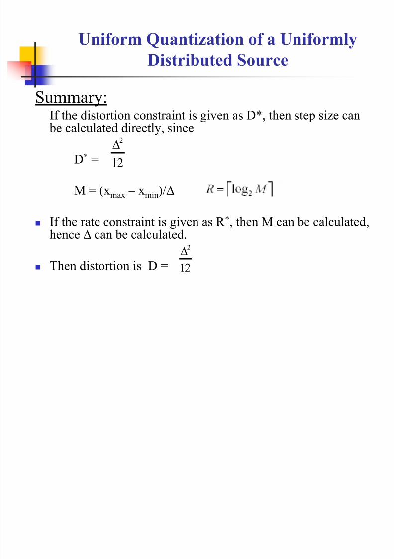
Summary:If the distortion constraint is given as D*, then step size can
be calculated directly, since
D* =
M = (xmax – xmin)/
If the rate constraint is given as R *, then M can be calculated,hence can be calculated.
Then distortion is D =
12
2
12
2
8/10/2019 Lossy Compression III
http://slidepdf.com/reader/full/lossy-compression-iii 19/49
8/10/2019 Lossy Compression III
http://slidepdf.com/reader/full/lossy-compression-iii 20/49
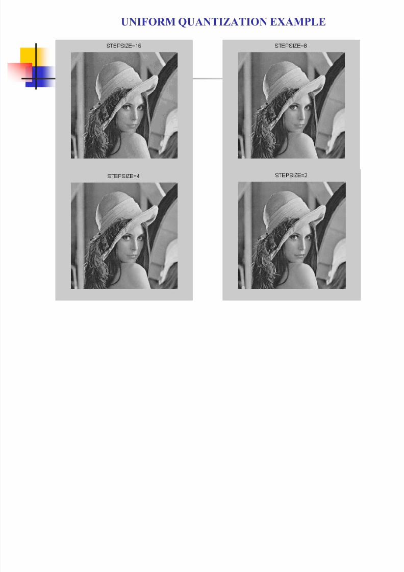
UNIFORM QUANTIZATION EXAMPLE
8/10/2019 Lossy Compression III
http://slidepdf.com/reader/full/lossy-compression-iii 21/49
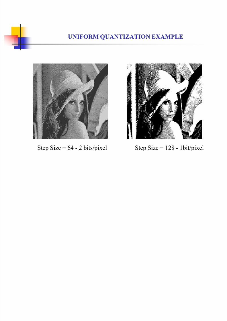
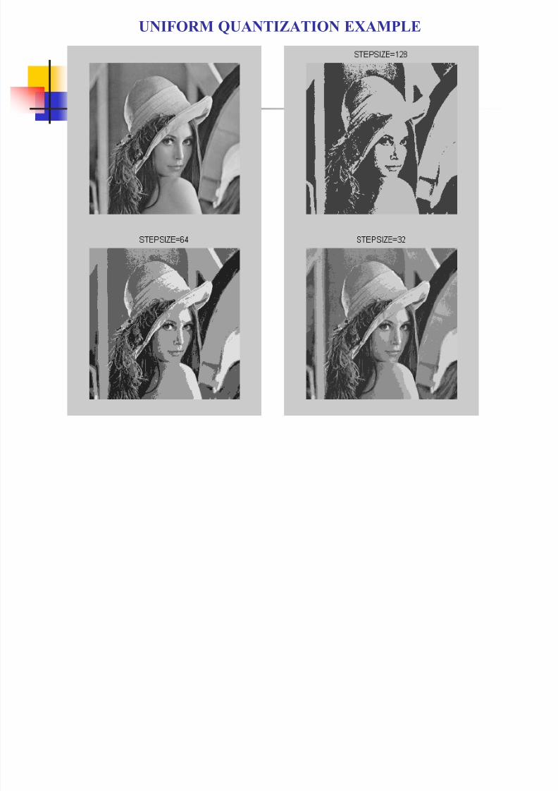
UNIFORM QUANTIZATION EXAMPLE
Step Size = 64 - 2 bits/pixel Step Size = 128 - 1bit/pixel
8/10/2019 Lossy Compression III
http://slidepdf.com/reader/full/lossy-compression-iii 22/49
Uniform Quantization of Non uniform
Sources
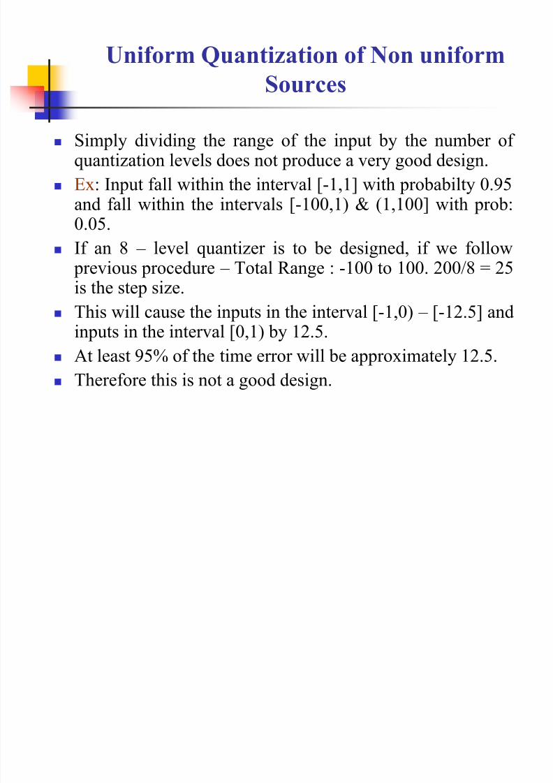
Simply dividing the range of the input by the number ofquantization levels does not produce a very good design.
Ex: Input fall within the interval [-1,1] with probabilty 0.95and fall within the intervals [-100,1) & (1,100] with prob:0.05.
If an 8 – level quantizer is to be designed, if we follow previous procedure – Total Range : -100 to 100. 200/8 = 25
is the step size. This will cause the inputs in the interval [-1,0) – [-12.5] and
inputs in the interval [0,1) by 12.5.
At least 95% of the time error will be approximately 12.5.
Therefore this is not a good design.
8/10/2019 Lossy Compression III
http://slidepdf.com/reader/full/lossy-compression-iii 23/49
Uniform Quantization of Non uniform
Sources
But if the step size that we select is small
say 0.3, then 95% of the time error will beless. But the rate will be very large.
Therefore if we have a non-uniformdistribution, we should include the pdf of
the source to determine the step size of a
Uniform Quantizer.
8/10/2019 Lossy Compression III
http://slidepdf.com/reader/full/lossy-compression-iii 24/49
8/10/2019 Lossy Compression III
http://slidepdf.com/reader/full/lossy-compression-iii 25/49
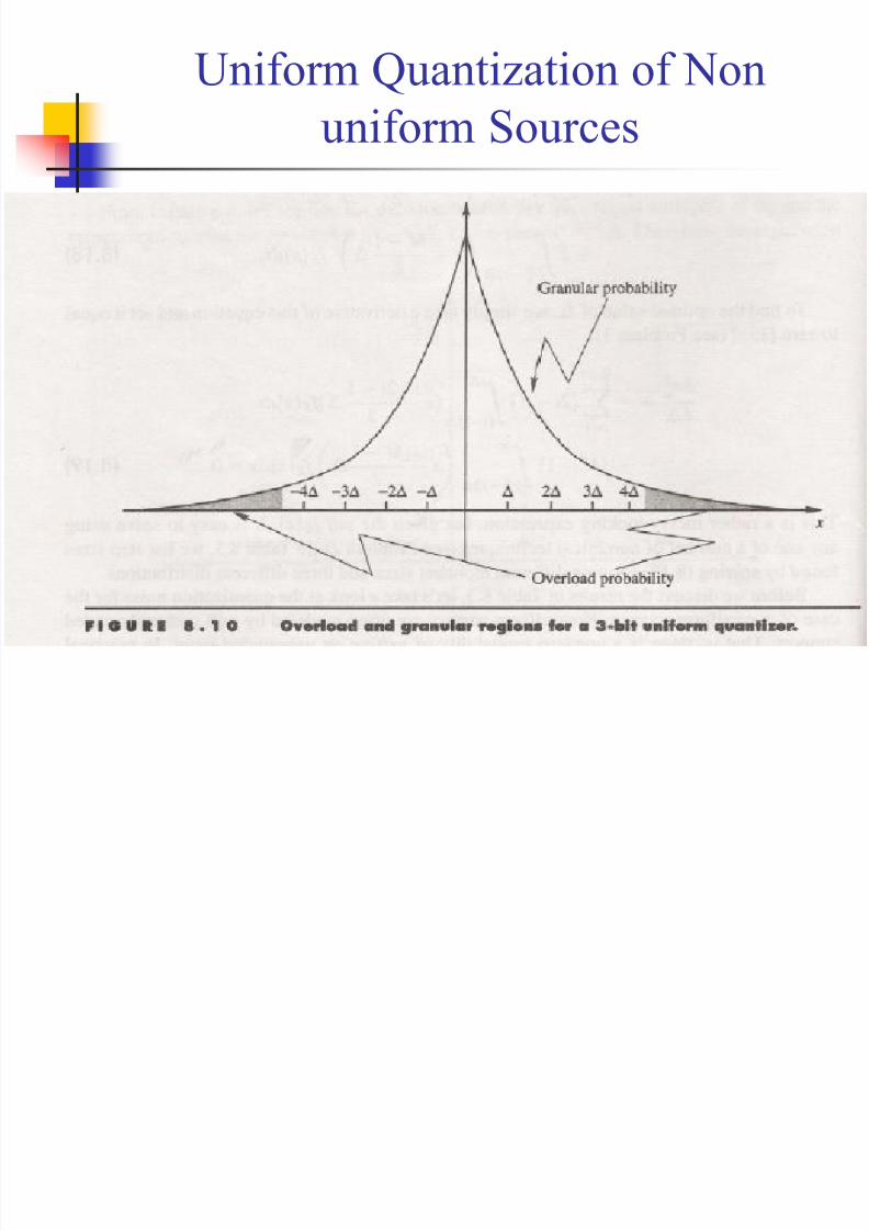
Uniform Quantization of Non
uniform Sources
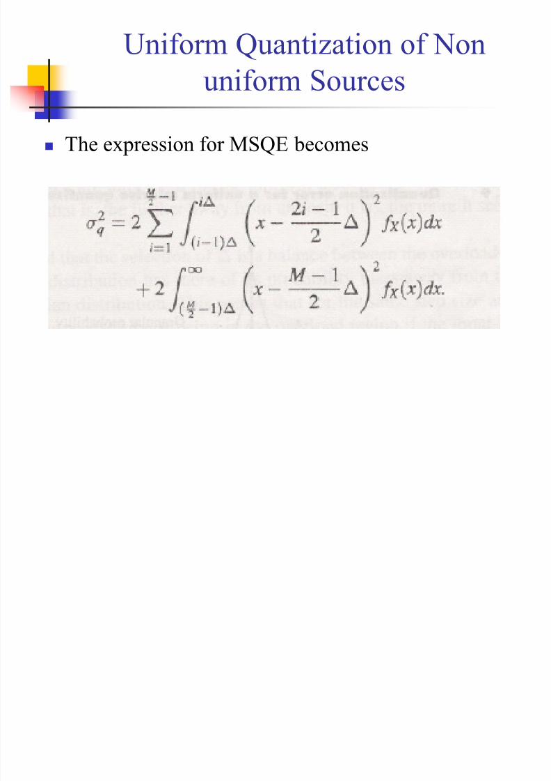
The expression for MSQE becomes
8/10/2019 Lossy Compression III
http://slidepdf.com/reader/full/lossy-compression-iii 26/49
8/10/2019 Lossy Compression III
http://slidepdf.com/reader/full/lossy-compression-iii 27/49
Uniform Quantization of Non
uniform Sources
8/10/2019 Lossy Compression III
http://slidepdf.com/reader/full/lossy-compression-iii 28/49
Uniform Quantization of Non
uniform Sources
8/10/2019 Lossy Compression III
http://slidepdf.com/reader/full/lossy-compression-iii 29/49
8/10/2019 Lossy Compression III
http://slidepdf.com/reader/full/lossy-compression-iii 30/49
Uniform Quantization of Non
uniform Sources
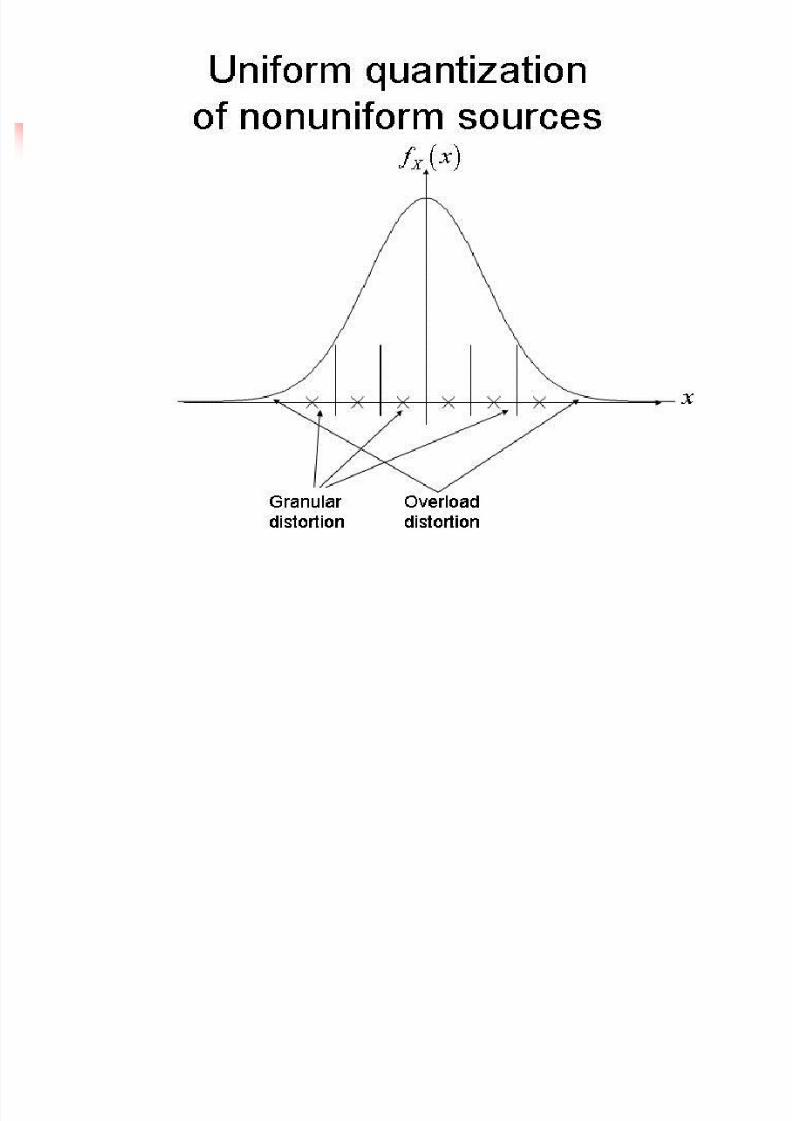
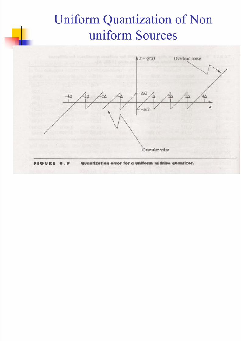
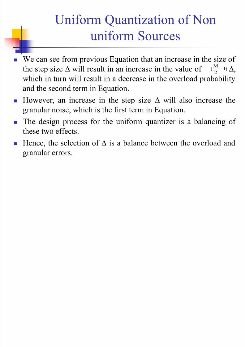
We can see from previous Equation that an increase in the size of
the step size will result in an increase in the value of ,
which in turn will result in a decrease in the overload probability
and the second term in Equation.
However, an increase in the step size will also increase the
granular noise, which is the first term in Equation.
The design process for the uniform quantizer is a balancing of
these two effects.
Hence, the selection of is a balance between the overload and
granular errors.
)12
M(
8/10/2019 Lossy Compression III
http://slidepdf.com/reader/full/lossy-compression-iii 31/49
UNIFORM QUANTIZATION EXAMPLE
8/10/2019 Lossy Compression III
http://slidepdf.com/reader/full/lossy-compression-iii 32/49
Non Uniform Quantization
If the input distribution has more mass near the origin,the input is more likely to fall in the inner levels of thequantizer.
Recall that in lossless compression, in order to minimizethe average number of bits per input symbol, we assignshorter code words to symbols that occurred with higher
probability and longer code words to symbols thatoccurred with lower probability.
In an analogous fashion, in order to decrease the average
distortion, we can try to approximate the input better inregions of high probability, at the cost of worseapproximations in regions of lower probability.
We can do this by making the quantization intervalssmaller in those regions that have more probability mass.
E l f if i
8/10/2019 Lossy Compression III
http://slidepdf.com/reader/full/lossy-compression-iii 33/49
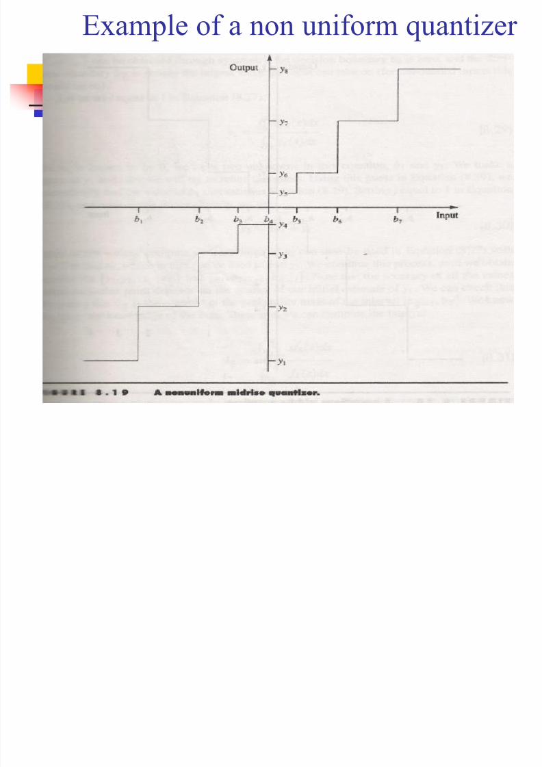
Example of a non uniform quantizer

8/10/2019 Lossy Compression III
http://slidepdf.com/reader/full/lossy-compression-iii 34/49
Optimization
We want to select the output levels (decision
levels) and decision thresholds (decision
boundaries) to minimize the distortion. Thereforewe write the distortion as a function the two.
dx x f y x
dx x f xQ x xQ x E
X
M
i
b
b
i
X q
i
i
)()(
)())(())((
1
2
222
1
8/10/2019 Lossy Compression III
http://slidepdf.com/reader/full/lossy-compression-iii 35/49
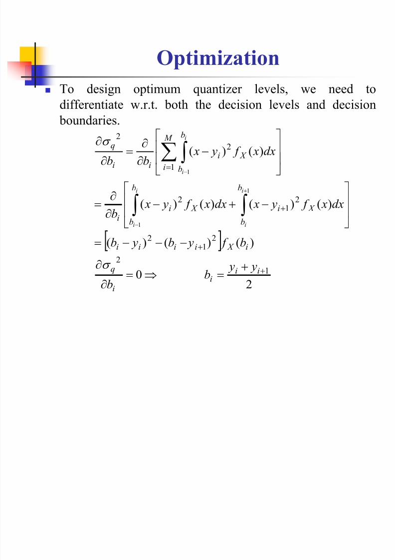
Optimization
To design optimum quantizer levels, we need to
differentiate w.r.t. both the decision levels and decision
boundaries.
20
)()()(
)()()()(
)()(
1
2
21
2
2
1
2
1
22
1
1
1
ii
ii
q
i X iiii
b
b X i
b
b X i
i
M
i
b
b
X iii
q
y y
bb
b f yb yb
dx x f y xdx x f y xb
dx x f y xbb
i
i
i
i
i
i
8/10/2019 Lossy Compression III
http://slidepdf.com/reader/full/lossy-compression-iii 36/49
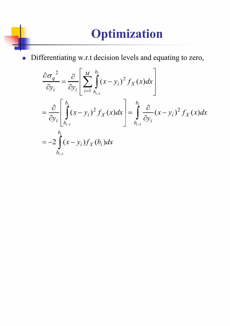
Optimization
Differentiating w.r.t decision levels and equating to zero,
dxb f y x
dx x f y x y
dx x f y x y
dx x f y x y y
i X
b
b
i
b
b
X i
i
b
b
X i
i
M
i
b
b
X iii
q
i
i
i
i
i
i
i
i
)()(2
)()()()(
)()(
1
11
1
22
1
2
2

8/10/2019 Lossy Compression III
http://slidepdf.com/reader/full/lossy-compression-iii 37/49
8/10/2019 Lossy Compression III
http://slidepdf.com/reader/full/lossy-compression-iii 38/49
8/10/2019 Lossy Compression III
http://slidepdf.com/reader/full/lossy-compression-iii 39/49
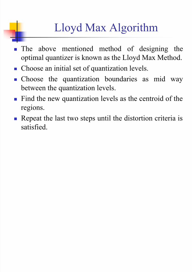
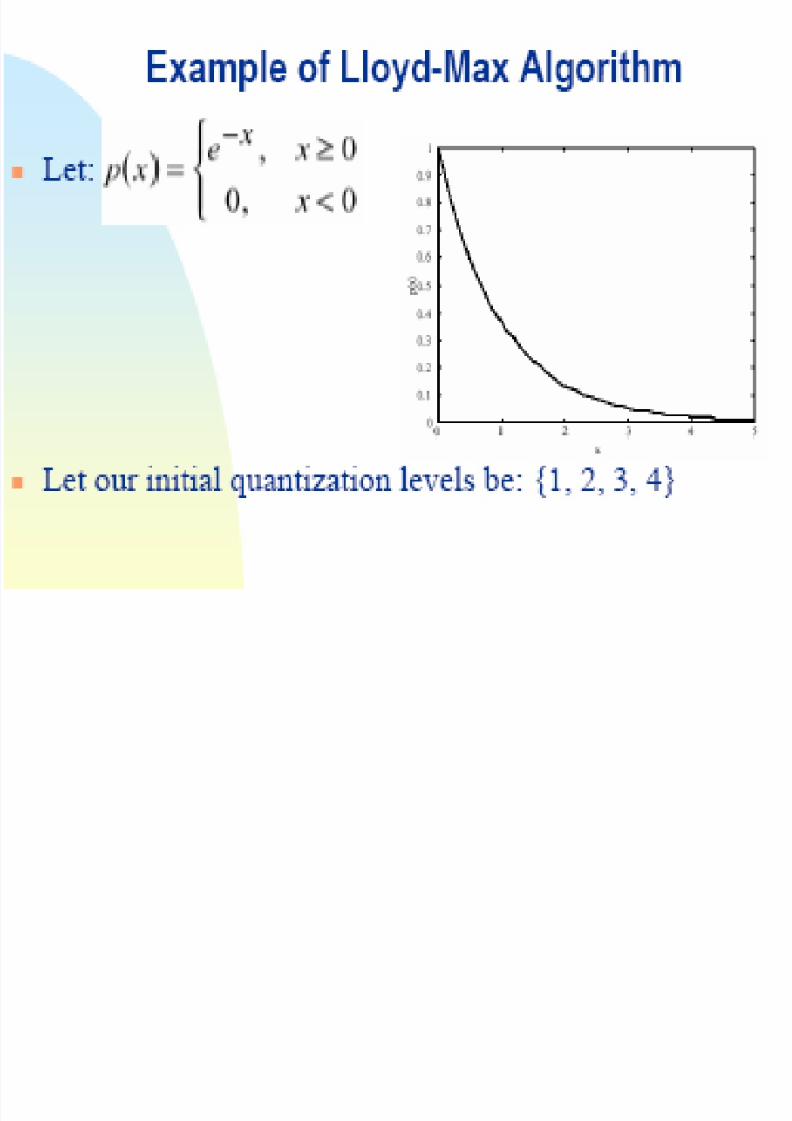
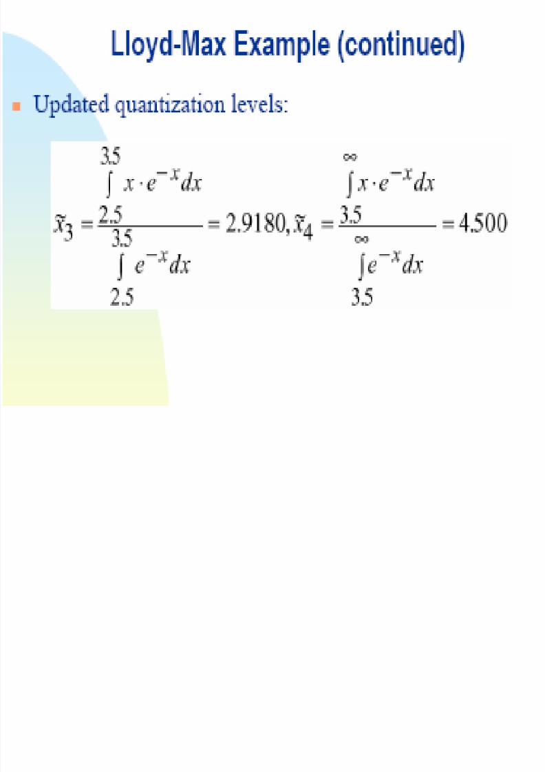
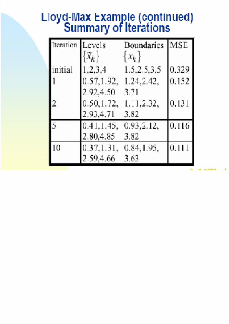
Lloyd Max Algorithm
The above mentioned method of designing the
optimal quantizer is known as the Lloyd Max Method.
Choose an initial set of quantization levels. Choose the quantization boundaries as mid way
between the quantization levels.
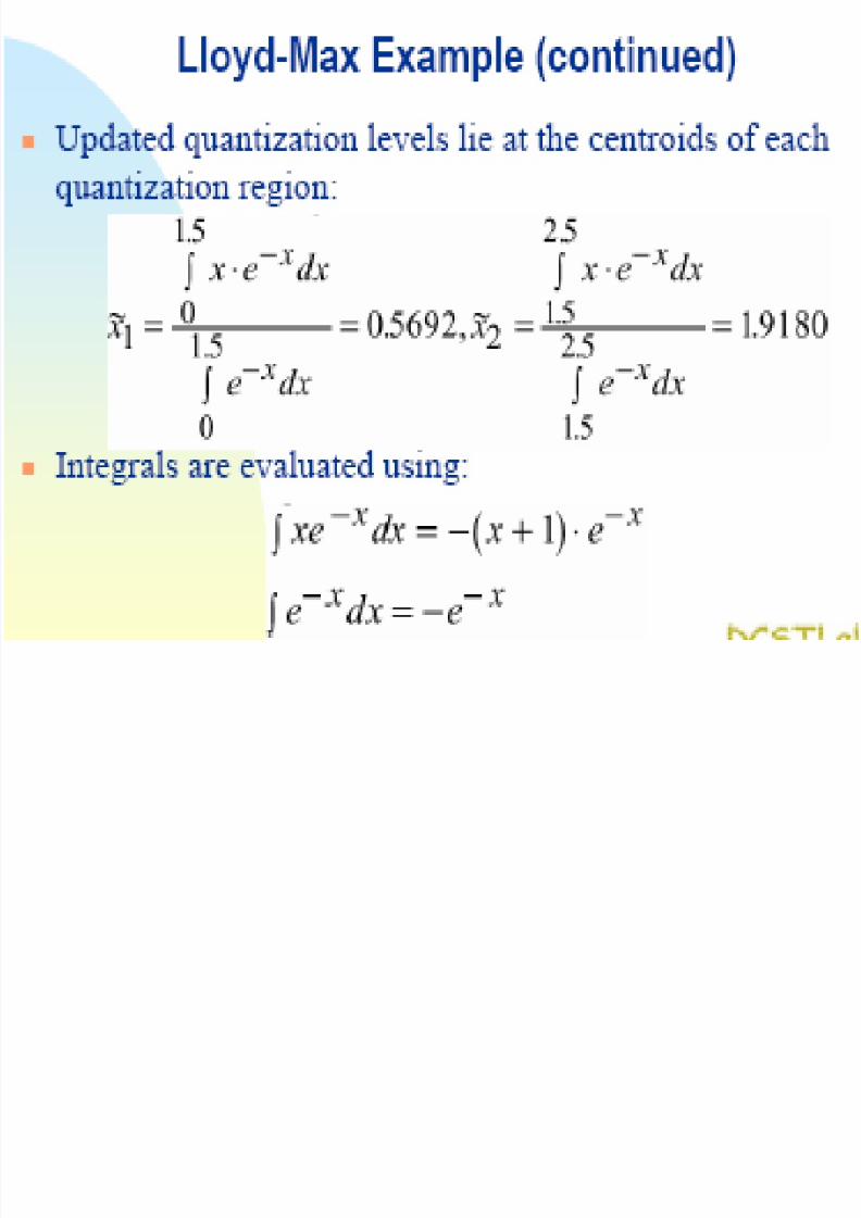
Find the new quantization levels as the centroid of theregions.
Repeat the last two steps until the distortion criteria is
satisfied.
8/10/2019 Lossy Compression III
http://slidepdf.com/reader/full/lossy-compression-iii 40/49
Non-Uniform Quantization
(Summary)
Entropy Coding – Shorter Code words to symbols with higher probability and longer code words to symbols with lower probability to minimize the average number of bits/ symbol.
Similarly, in waveform coding using non-uniform quantizer,we approximate the input better in regions of higher
probability at the cost of worse approximations in regions oflower probability.
By making the quantization intervals smaller in those regionsthat have more probabilty mass.
If we want to keep the number of intervals constant, we uselarger intervals away from the origin.
Lloyd-Max method – pdf – optimized quantization
8/10/2019 Lossy Compression III
http://slidepdf.com/reader/full/lossy-compression-iii 41/49
Companded Quantization
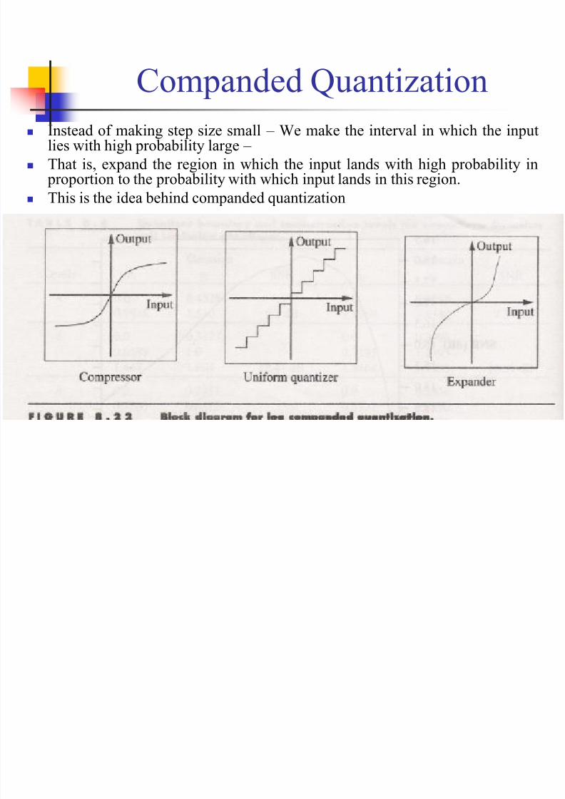
Instead of making step size small – We make the interval in which the inputlies with high probability large –
That is, expand the region in which the input lands with high probability in proportion to the probability with which input lands in this region.
This is the idea behind companded quantization
8/10/2019 Lossy Compression III
http://slidepdf.com/reader/full/lossy-compression-iii 42/49
Companded Quantization Cont..
The input is first mapped through a compressor function.
This function "stretches" the high-probability regions close tothe origin, and correspondingly compresses the low-probabilityregions away from the origin.
Thus, regions close to the origin in the input to the compressoroccupy a greater fraction of the total region covered by thecompressor.
If the output of the compressor function is quantized using auniform quantizer, and the quantized value transformed via anexpander function, the overall effect is the same as using a nonuniform quantizer.
8/10/2019 Lossy Compression III
http://slidepdf.com/reader/full/lossy-compression-iii 43/49
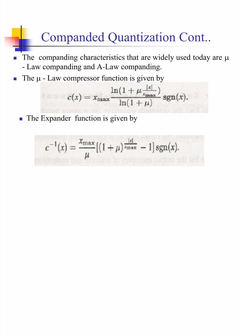
The companding characteristics that are widely used today are
- Law companding and A-Law companding.
The - Law compressor function is given by
The Expander function is given by
Companded Quantization Cont..
8/10/2019 Lossy Compression III
http://slidepdf.com/reader/full/lossy-compression-iii 44/49
Companded Quantization Cont..
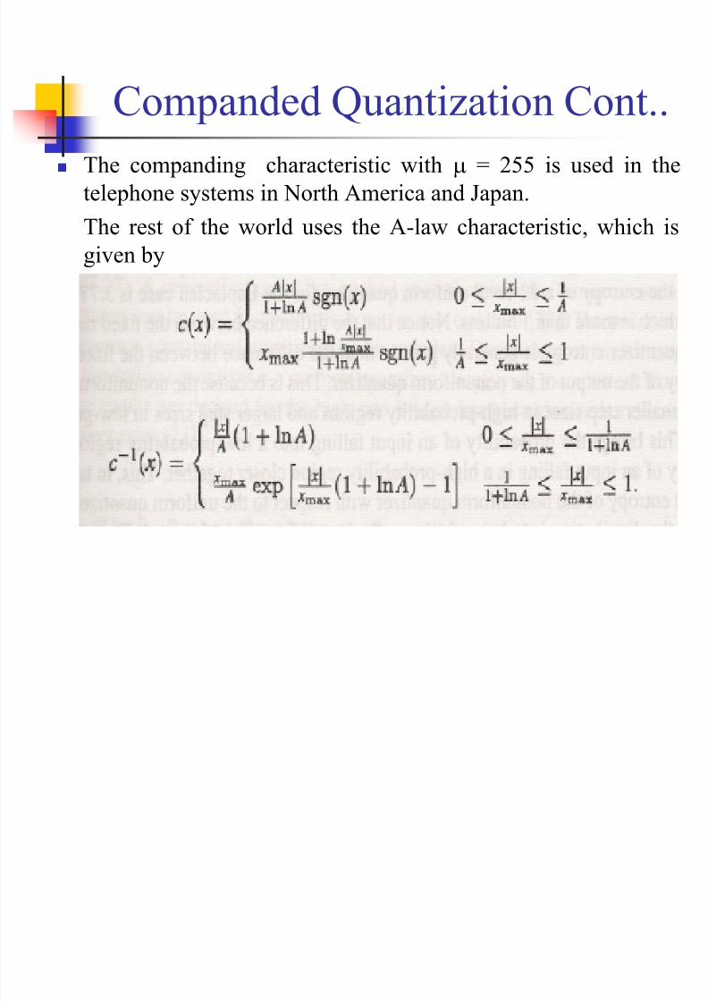
The companding characteristic with = 255 is used in the
telephone systems in North America and Japan.
The rest of the world uses the A-law characteristic, which is
given by
8/10/2019 Lossy Compression III
http://slidepdf.com/reader/full/lossy-compression-iii 45/49
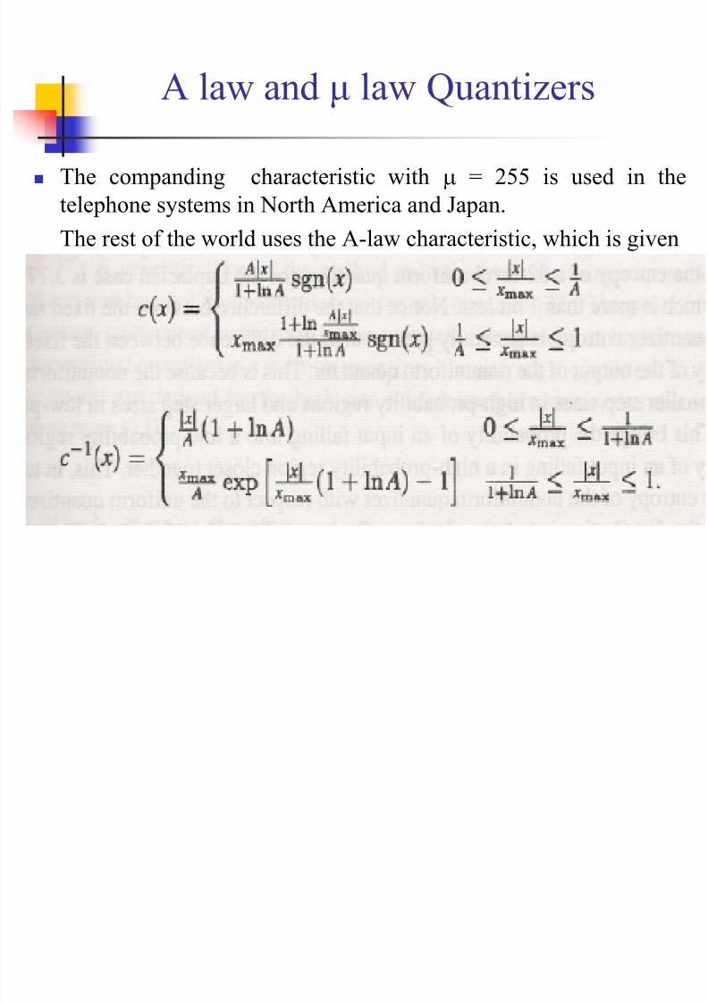
The companding characteristic with = 255 is used in the
telephone systems in North America and Japan.
The rest of the world uses the A-law characteristic, which is given
by
A law and μ law Quantizers
8/10/2019 Lossy Compression III
http://slidepdf.com/reader/full/lossy-compression-iii 46/49
8/10/2019 Lossy Compression III
http://slidepdf.com/reader/full/lossy-compression-iii 47/49
8/10/2019 Lossy Compression III
http://slidepdf.com/reader/full/lossy-compression-iii 48/49
8/10/2019 Lossy Compression III
http://slidepdf.com/reader/full/lossy-compression-iii 49/49